Techno-economic model for long-term revenue prediction in distribution grids incorporating distributed energy resources

Distributed energy resources (DER) is a prevalent technology in distribution grids. However, it poses challenges for distribution network operators to make optimal decisions, estimate total investment returns, and forecast future grid operation performance to achieve investment development objectives. Conventional methods mostly rely on current data to conduct a static analysis of distribution network investment, and fail to account for the impact of dynamic variations in relevant factors on a long-term scale on distribution network operation and investment revenue. Therefore, this paper proposes a techno-economic approach to distribution networks considering distributed generation. First, the analysis method of the relationship between each investment subject and distribution network benefit is established by using the system dynamics model, and the indicator system for distribution network investment benefit analysis is constructed. Next, the distribution network operation technology model based on the dist flow approach is employed. This model takes into account various network constraints and facilitates the comprehensive analysis of distribution network operation under dynamic changes in multiple factors. Consequently, the technical index parameters are updated to reflect these changes. This updated information is then integrated into the system dynamics model to establish an interactive simulation of the techno-economic model. Through rigorous verification using practical examples, the proposed method is able to obtain the multiple benefits of different investment strategies and be able to select the better solution. This can provide reference value for future power grid planning.

1 Introduction

Distributed energy resources (DER) is widely regarded as one of the important renewable energy generation modes in the distribution network (International Energy Agency, 2022). The distribution network characterized by accepting large-scale renewable energy has become the main trend and direction of the future development of the distribution network. DG has changed the energy flow mode of the traditional distribution network, which brings great challenges to the economy, reliability and power quality of the distribution network (Dhivya and Arul, 2021). DER integration challenges distribution investment optimization and return estimation. Uncertain DER generation output complicates infrastructure planning. Bidirectional power flows from DERs require investments to manage voltage, loading, and protection. DERs cause voltage fluctuations potentially exceeding regulations, needing voltage regulation equipment. Varying DER loading causes asset under/over-utilization. Long planning horizons with rapidly adopting DERs make forecasting difficult. Therefore, effective and reasonable distribution network investment planning is the necessary condition to solve the above problems (Yi et al., 2021). How to fully consider the influence of DG on the distribution network and make reasonable investment decisions is one of the core tasks of distribution network planning under the condition of limited investment (Maheshwari et al., 2020).

Academics endeavor to address the challenges presented by the integration of distributed renewable resources into the distribution network through the interactive operation of generators, networks, and energy storage systems. Literature (Ehsan and Yang, 2019) evaluates uncertainty modeling techniques within the framework of active distribution network planning and discusses their additional challenges and solutions. Literature (Adefarati and Bansal, 2019) evaluates the reliability, environmental, and economic impacts of several case studies using the fmincon optimization tool in MATLAB. Literature (Panigrahi et al., 2020) introduces control methods for small photovoltaic power stations and several aspects of grid-connected photovoltaic systems, ranging from various standards to emergency operations. Literature (Luo et al., 2020) proposes a RES management approach applicable to different RES distribution networks and attempts to find the optimal energy management of grid-connected distribution networks using an improved bat algorithm (MBA). Literature (Cui et al., 2019) aims to improve the revenue of distributed wind power generation (DWPG) and reduce grid upgrade costs by establishing a model considering the collaborative planning of distributed wind power generation and distribution networks.

The above literature mainly focuses on planning distribution networks that maximize the economic benefits while considering the uncertainty of renewable energy, grid constraints, and the integration of distributed energy resources. These methods can only provide investment in the current form of the distribution network on a certain investment basis. In reality, the investment in the distribution network is interrelated and is dynamically affected by various factors such as load growth, DER growth, and GDP over a long period (Thang, 2021). Traditional optimization methods cannot represent the long-term effects of multiple dynamic external factors on the demand of distribution networks. Moreover, it cannot analyze the long-term overview of distribution networks and consider the investment return expectations of these factors.

System dynamics is an ideal method for solving long-term forecasting problems involving multiple factors and complex feedback. Moreover, it has been widely applied in power systems (Teufel et al., 2013). For instance (Song et al., 2021), constructed a system dynamics model for a multi-market coupled trading system to study the coupling effects of multiple factors on renewable energy sources (RES) evolution (Li et al., 2022). developed a system dynamics model to predict long-term loads considering carbon neutrality targets (Tang et al., 2021). used system dynamics to predict power generation combinations on the rolling horizon and employed it as a forecasting method considering multiple factors. Furthermore, system dynamics can be employed to analyze the impact of certain variables on the system (Ying et al., 2020). used system dynamics to study demand-side incentives under renewable energy portfolio standards. Similarly (Chi et al., 2022), applied system dynamics to analyze carbon emissions under electricity market reform, which indicates that future market electricity prices will show advantages in efficiency and liquidity.

However, there exist multiple short-term operational constraints in distribution networks. System dynamics is a long-term simulation tool, and many constraints cannot be calculated, leading to invalid or even incorrect results. In this case, some scholars propose using integrated models with system dynamics to address its limitations (Tang et al., 2021). combined rolling horizon optimization with a system dynamics model to predict the evolution of power generation combinations. Although the article proposed a calculation model that integrates system dynamics with other methods, the problem of limited computation remains unsolved. The dynamic correlation among a large number of complex factors in long-term models and the operational constraints in short-term models cannot be reconciled and need further research (Ying et al., 2020).

This paper presents a simulation method of distribution network planning investment based on dual time scale fusion. The system dynamics is used as the long-term simulation, and the optimal power flow calculation model of the distribution network is used as the short-term simulation. First, based on the demand of economic and social development for regional distribution network planning, the main influencing factors of distribution network planning investment are screened out, and the multi-factor complex system is modeled through system dynamics. Secondly, the optimal power flow calculation is introduced, and some key parameters of the system dynamics are introduced and solved. The short-term simulation verifies the operation constraints of the distribution network in the long-term evolution, and obtains the profit value of various investments. The results can be returned to the system dynamics model to obtain more valuable long-term inference conclusions. The proposed techno-economic approach provides an advanced, adaptive framework for long-term distribution investment analysis, overcoming limitations of conventional techniques. It uses system dynamics modeling to capture long-term trends rather than static optimization. It incorporates complex interdependent impacts on investments over time that conventional methods miss. Integration of the dist flow model represents network constraints lacking in traditional approaches. Closed loop updating of system dynamics with the dist flow method enables adaptive decisions, improving on conventional inflexibility.

The main contributions of this paper are summarized as follows:

1. Traditional optimization models are unable to capture the dynamic impacts of various factors on the long-term investment returns of distribution networks. In this paper, a long-term simulation model is designed that utilizes system dynamics to model the long-term trends of relevant factors. The resulting outcomes can more effectively infer the long-term evolution trend of the distribution network over a longer time scale.

2. There are multiple constraints in the operation of distribution networks, and traditional system dynamics cannot perform constraint calculations. In this paper, a dual-time-scale simulation model is designed. System dynamics is used for long-term simulation, while key parameters related to power system constraints are calculated through optimal power flow constraint for short-term simulation. This can address the limitations of system dynamics.

3. A comprehensive investment return evaluation index system is constructed in this paper. The evaluation indexes are calculated based on the results of short-term simulations, while the changes in these indexes’ impact on the long-term evolution of the distribution network are characterized through long-term simulation. This method is only applicable to dual-time-scale simulation models and can provide decision-makers with intuitive investment return references.

2 System dynamics model

Distribution network investment decision is a multi-objective decision problem, which is also a multi-stage planning problem in a long time scale. The entity responsible for the distribution network investments being modeled and analyzed in this study can be the distribution system operator or utility company that owns and operates the network assets. The model outputs aim to inform their long-term planning and investment decisions. The decision goals are of various types. Some indicators are as large as possible, such as the user power supply reliability rate, voltage compliance rate, and some are neither larger nor smaller, such as power supply per unit variable capacity. To transform the multi-attribute decision problem into a single attribute decision problem can effectively improve the efficiency and accuracy of the solution. The core idea is to unify the evaluation indicators of different dimensions into the same dimension by normalization and weighting.

The investment in regional distribution network is often affected by demand. The greater the demand for a certain benefit, the greater the investment necessity and the greater the investment scale for relevant measures. However, restricted by the actual investment of the power network, the investment limit cannot be exceeded. In addition, since the distribution network requires balanced development to some extent, each benefit of the distribution network should complete its basic distribution network planning objectives, and some benefits of the distribution network should not be ignored in order to improve the comprehensive benefits of the distribution network, which is also an important constraint for investment decisions. The investment demand, investment capacity and basic planning objectives of each benefit of distribution network are considered comprehensively.

In this paper, system dynamics is used to construct a long-term simulation model for the evolution of distribution network. The construction process is:

1. Defined boundaries and assumptions;

2. Construct the causal loop diagram;

3. Define sub-systems and construct the stock flow chart.

2.1 Model boundary and assumptions

The first step to construct a functional SD model is to define the boundaries and assumptions of the model. The research object of this paper is grid distribution network. It refers to the distribution network divided by geographical and administrative units within a certain area. Due to regional development, natural conditions, grid company assessment and other factors, the distribution network conditions are different. By subdividing a large area into a grid distribution network, the difficulty of analysis can be reduced by subdividing analysis objects. Grid distribution network has the following characteristics:

1. The power supply mode of the distribution network changes from single source to multi-source, and the average load rate and the distribution transformer capacity load ratio of the distribution network change. The transmission power along the feeder decreases, and the voltage at each node increases. The change depends on the volume and location of DG.

2. The uncertainty of DG output leads to voltage fluctuations in the distribution network, and energy storage and other devices need to be added to suppress fluctuations;

3. DG is generally incorporated into the power grid through the inverter, which will produce a large number of harmonic components. This will change the voltage and current waveform of the distribution network, causing harmonic pollution, need to add a filtering device;

4. Two-way transmission of distribution network, traditional protection devices are difficult to identify and troubleshoot faults, which increases the investment demand of secondary system of distribution network.

Based on the above features, the model boundary and assumptions in this paper are as follows:

1. This paper mainly studies the distribution network with distributed power supply. The proposed model is not suitable for the distribution network without DG.

2. For the verification of grid fees for distributed energy, it is necessary to comprehensively consider the grid assets, voltage levels, and electrical distances occupied by both parties in the market-oriented transaction of distributed generation under the market-oriented trading of electricity. At present, however, Chinese electric power market is not completely popular. In this case, most distributed power sources do not participate in the electricity market, so they ignore the impact of the electricity market.

3. Electric vehicles and distributed energy storage are not included in the model.

4. Assume that the type of equipment invested in the distribution network is fixed and the investment cost is unchanged.

2.2 Casual loop diagram

The casual loop diagram of the model is shown in the Figure 1. Based on the casual loop diagram, the model can be divided into three subsystems.

1. Distribution network investment subsystem. This module simulates the growth of various types of equipment in the distribution network. Key elements include: distributed energy storage, static var compensator, transformer, line capacity.

2. End user subsystem. This module simulates distribution network user demand and DER growth. Key elements include: DER, peak load, electricity demand, GDP growth.

3. Revenue calculation subsystem. This module simulates the growth of distribution network revenue. Among them, the short-term simulation model is included, that is, the optimal power flow calculation model. Key elements include: power quality, power self-supply rate, RES consumption rate, line load rate, and network loss rate.

FIGURE 1

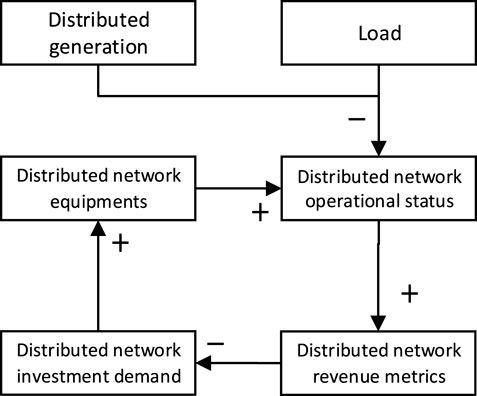
FIGURE 1. Casual loop diagram.

2.3 Stack-flow model

In the SD model, the quantitative relationship between variables are characterized by a stack flow model. This section details the above three sub-system formulations, as shown in Figure 2.

FIGURE 2

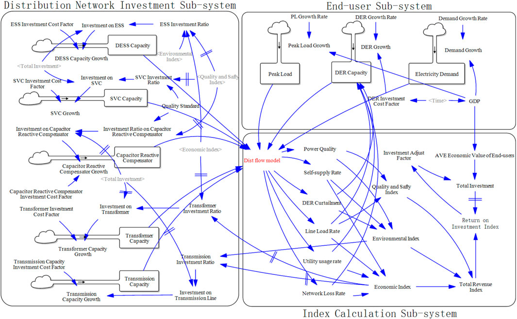
FIGURE 2. Stack-flow model.

2.3.1 Distribution network investment subsystem

There are five types of distribution network investment objects in this paper. They are DESS, SVC, CRC, transformer and transmission line. The type of DESS in this paper is electrochemical energy storage such as lithium-ion and flow batteries, which are common distribution-level storage technologies. State of charge constraints limit usable capacity. Storage decision variables are charge/discharge amounts, State-of-Charge, and charging/discharging status. For each investment object, it is represented by the corresponding stock variable, which is an integral function based on the growth variable.

$CA{P}_i\left(t\right)=CA{P}_i\left(t-1\right)\times \left(1+I{V}_i\right),i\in ESS,SVC,CRC,T,L(1)$

$I{V}_i=\frac{RF}{IV{F}_i},i\in ESS,SVC,CRC,T,L(2)$

where, IV is the investment index defined as the ratio of current capacity.

Investment decisions should be based on economic indicators of investment profitability. In this paper, the investment decision is made through the revenue index RF whose calculation process is similar to net profit value (NPV) (Petitet et al., 2017).

$RF={\displaystyle \sum _{t=0}^n}\frac{R_i-C_i}{{\left(1+dis\right)}^t}-IV{F}_i,i\in ESS,SVC,CRC,T,L(3)$

where dis is a discount factor of 5%, n is the time period which is 20 years in this paper, R_i is presented in Eq. 18.

The growth of DER is influenced not only by cost and technological factors but also by operational indicators of the distribution network. Among these indicators, energy self-sufficiency and the integration rate of renewable energy are the two most important ones. The relationship between these indicators is as follows:

$CA{P}_{\mathit{DER}}\left(t\right)=CA{P}_{\mathit{DER}}\left(t-1\right)\times \left(1+r_{\mathit{DER}}\right)(4)$

$r_{\mathit{DER}}={\alpha }_1\times \left(1+\left(1-{\eta }_s\right)+{\alpha }_2\times {\eta }_{D}ER\right)(5)$

2.3.2 Revenue calculation subsystem

This module focuses on income calculation. First, various operating parameters of the distribution network are calculated through short-term simulation, and then the parameters are converted into income-related coefficients. The short-term simulation model refers to Section 3. This section focuses on the modeling of profitability parameters.

Power quality:

The power supply quality index of distribution network is similar to that of distribution network, which reflects the average power quality of distribution network. In this paper, the power quality indexes of load access nodes and grid-connected nodes of distribution network are averaged in time and space to reflect the characteristics of power supply quality in statistical time of distribution network. For example, the formula for calculating the mean value of voltage deviation degree and three-phase voltage unbalance degree is respectively

$ND={\displaystyle \sum _{t=1}^T}{\displaystyle \sum _{n=1}^N}\left|\delta U_n\left(t\right)\left(\%\right)\right|/\left(N\times T\right)(6)$

${\eta }_U=\frac{U_{\text{m}}-U_{\text{N}}}{U_{\text{N}}}\times 100\%(7)$

Self-supply rate:

The self-smoothness of energy represents the self-sufficiency capacity of the distribution network, which is expressed by the ratio of the self-consumed electricity of the distribution network to the total load power supply within the statistical time, and the calculation formula is

${\eta }_s={\int }_{i=1}^t\left(1-\frac{E_i^{\mathrm{P}\mathrm{C}\mathrm{C}}}{E_i^{\mathrm{L}\mathrm{o}\mathrm{a}\mathrm{d}}}\right)\mathrm{d}i/t\times 100\text{\%\hspace{0.17em}}(8)$

Reliability benefit:

Average percentage of power supply shortage of users. The ratio of average power failure to power failure of users represents the power failure of users, and is expressed by the ratio of total power failure to power failure within the statistical period and the expected power failure within the statistical period, where the expected power failure is the sum of actual power supply and power failure, and the statistical period is 1 year.

${\eta }_r=c_l*LOLE(9)$

where c_l is the cost index of non-served energy; LOLE is loss of load expectation;

The benefit-cost ratio η of distributed energy access to the grid is defined as the ratio of the annual power outage loss cost change value Δ Closs to the annual investment cost C_invest.

$\eta =\mathrm{\Delta }{C}_{\text{loss\hspace{0.17em}}}/C_{\text{invest\hspace{0.17em}}}(10)$

It is used to quantify the improvement benefits of various access methods to the distribution network reliability index, sort and compare the benefit-cost ratio, and obtain the best benefit measures.

Line load rate:

Line load factor is the ratio of actual load to rated capacity. It evaluates line performance, guides planning, improves energy efficiency, and aids in operational management in power systems.

${\eta }_a=\frac{S_a}{S_0}\times 100\text{\%\hspace{0.17em}}(11)$

where η_a is the distribution network load rate level of the system; S_a is the average load capacity of the distribution network; S₀ is the rated load capacity of the distribution network.

Utility usage rate:

Equipment utilization is an index that can reflect the working status and production efficiency of the equipment in the system, and has important evaluation significance. Equipment utilization refers to the ratio of the actual working time of the equipment to the planned working time within a certain period of time. The value of this value is directly related to the project benefit. The specific expression is:

${\eta }_e=\left({\displaystyle \sum _{n=1}^N}{T}_n\right)/(N{T}_O)(12)$

where η_e is the equipment utilization rate of the system; T_O is the unit planned working hours; T_n is the actual working hours of the first device in a unit time; N is the number of energy link equipment in the system.

DER curtailment:

The power abandonment rate of clean energy refers to the ratio of the product of the running time of each DG year (unit: h) and its installed capacity (unit: kW) in the distribution network to the rated power generation of each DG year due to the unstable wind power output. The calculation formula is

$R_{\text{DER\hspace{0.17em}}}=1-E_{\mathit{DER}}/E_{DER\text{\_}F}(13)$

${\eta }_{\mathit{DER}}={\int }_{i=1}^t\left(1-\frac{E_i^{\mathrm{D}\mathrm{E}\mathrm{R}}}{E_i^{\mathrm{D}\mathrm{E}\mathrm{R}\text{\_}\mathrm{F};}}\right)\mathrm{d}i/t\times 100\text{\%\hspace{0.17em}}(14)$

where R_DER is the curtailment rate of DER; E_DER is the actual grid-connected power generation; E_{DER_F} is the power generation.

Quality and safty index:

$R{F}_Q=1-\left(1-{\eta }_U\right)+{\eta }_r/{\beta }_1(15)$

Economic index:

$R{F}_{\mathit{ECO}}=\left(1-{\eta }_s\right)+{\eta }_r/{\beta }_2(16)$

Environment index:

$R{F}_{EN}=\left(1-{\eta }_s\right)+\left({\eta }_a/{\beta }_3\right)+\left(1-{\eta }_e\right)-\left(1-{\eta }_{\mathit{DER}}\right)(17)$

Total revenue index: In the indicator system of this paper, weights are added to the three indicators respectively, expressed as

$RF={\alpha }_1\times R{F}_Q+{\alpha }_2\times R{F}_{\mathit{ECO}}+{\alpha }_3\times R{F}_{EN}(18)$

where α₁, α₂, and α₃ are weight factors.

2.3.3 End user subsystem

This module is mainly based on external variables. Including electricity demand, peak load, DER capacity. Among them, DER capacity is affected by other module variables, while power demand and peak load are purely external input variables.

$ED\left(t\right)=ED\left(t-1\right)\times \left(1+r_{ED}\right)(19)$

$r_{ED}=e_1*Ln\left(e_2\times \left(Time-2020\right)\right)(20)$

where ED is the electricity demand; r_ED and r_PL represents the growth rate of electricity demand and peak load, respectively. Note that e₁ and e₂ are 0.05 and −0.03427 in this paper, which are calculated by fitting historical data from the past 20 years.

The peak load variable is critical in the system dynamics model, directly affecting distribution network infrastructure sizing and operation simulated by the dist flow model. Larger peak load requires increased capacity components and equipment ratings to handle maximum flows. Peak demand drives asset utilization and overloading risk analysis in the dist flow. It also dictates voltage regulation needs, as bigger peaks cause larger voltage drops. Furthermore, peak load determines nodal demands and network flows in the dist flow. The annual peak load is influenced by various factors, which can be divided into two categories: trend changes and random fluctuations. Trend changes are influenced by policies and economic development, while random fluctuations are affected by load fluctuations and major events. Considering that the annual peak load exhibits a relatively stable trend growth, it can be viewed as a random variation, with random factors superimposed on the relatively stable trend changes, resulting in fluctuating randomness. As a result, the increase in load is uncertain, and the extent of variation is unpredictable.

$P_T=\frac{1}{\sqrt{2\pi }\sigma }\exp \left(-\frac{{\left(x-\left(1+a\right)\right)}^2}{2{\sigma }^2}\right)(21)$

where, a represents the growth rate of the long-term trend change, x denotes the growth rate of the current year, and the scale parameter is represented by σ.

3 Dist flow method

The utilization of an economic model within the system dynamics framework allows for the simulation of diverse investment growth scenarios. However, the accurate calculation of indicators necessitates a thorough analysis of operational data from the distribution network. In this context, the employment of an optimization model, integrated with engineering constraints, becomes imperative. It is worth noting that the system dynamics model cannot be effectively solved through constrained optimization techniques alone. Consequently, this paper introduces a novel linear power flow calculation model for multi-scenario distribution networks.

3.1 Dist flow model

The dist flow model, also known as the linear power flow calculation model, plays a crucial role in analyzing and optimizing the operation of distribution networks. This model provides significant benefits for power flow analysis in distribution networks compared to other methods. This model is employed to estimate the power flow and voltage profiles within the network, considering various constraints and operational conditions, as well as the impacts of DER such as solar panels, wind turbines, and energy storage systems. The dist flow model utilizes a linear approximation of the power flow equations, enabling efficient and computationally tractable solutions. It considers the voltage magnitudes and angles at different network nodes, reactive power flows, and real power losses. By solving this model, researchers and engineers can obtain valuable insights into network performance, voltage regulation, power losses, and the integration of renewable energy sources. Moreover, the distribution flow model serves as a fundamental tool for various applications, including network planning, voltage control, optimal DER placement, and analysis of fault conditions. Its integration with optimization algorithms allows for the identification of optimal operating strategies and the evaluation of investment decisions, considering factors such as cost, reliability, and environmental impact. This makes dist flow method low a versatile tool for applications in planning, voltage regulation, DER integration, and more.

3.1.1 Objective function

The objective function including the optimal power flow problem of DER distribution network generally includes the minimum loss of distribution network, the minimum node voltage deviation and the minimum DER operating cost. It can be expressed in the general form shown in Eq. 1.

$\min {\displaystyle \sum _{i=0}^n}{C}_i\left(P_{i,t},Q_{i,t},U_{i,t}\right)=C_{\text{loss\hspace{0.17em}}}+C_{\text{U}}+C_{\text{res}}+C_{\text{ess}}(22)$

where C_loss is the total loss. P_i,t and Q_i,t are respectively the active power and reactive power of injection at node i at time t; U_i,t is the voltage amplitude of node i at time t; C_i(⋅) is the cost function of node i, n is the total number of nodes.

The cost function contains 4 parts: distribution network loss, node voltage deviation, penalty cost for RES reduction, energy storage charge and discharge cost.

Distribution network loss:

$C_{\text{loss\hspace{0.17em}}}={\displaystyle \sum _{i=0}^n}{P}_{i,t}(23)$

That is, the distribution network loss is equal to the sum of the active power injections of all nodes including the root node.

Node voltage deviation:

$C_{\text{U}}={\displaystyle \sum _{i=1}^n}{c}_{\text{U}}{\left(U_{i,t}-U_{\text{base\hspace{0.17em}}}\right)}^2(24)$

where c_U is the node voltage amplitude deviation penalty coefficient; U_base is the voltage reference value, which can be taken as the voltage value of the root node.

Penalty cost of RES reduction:

Taking the photovoltaic power supply as an example, it is shown in formula 40.

$C_{\text{res}}=c_{\text{res}}\left(P_{i,t,\max }-P_{i,t}\right)(25)$

where C_res is the light abandonment penalty coefficient; P_i,t,max is the maximum active power of photovoltaic determined by the maximum power tracking technology at time t; i ∈ N_res, N_res is the set of renewable energy grid-connected nodes.

Energy storage charge and discharge cost:

$C_{\text{ess}}=c_{\text{ess}}{P}_{i,t}^2(26)$

where C_ess is the energy storage charge and discharge cost coefficient;i ∈ N_ess, N_ess is the set of energy storage grid-connected nodes.

3.1.2 Power flow constraint

${\displaystyle \sum _{j=1}^{N^i}}\left[U_i{U}_j\left(G_{ij}\cos {\theta }_{ij}+B_{ij}\sin {\theta }_{ij}\right)\right]=P_i(27)$

${\displaystyle \sum _{j=1}^{N^i}}\left[U_i{U}_j\left(G_{ij}\sin {\theta }_{ij}-B_{ij}\cos {\theta }_{ij}\right)\right]=Q_i(28)$

$P_i=P_i^{\text{line}}+P_i^{\text{dis}}-P_i^{\text{Load}}{Q}_i=Q_i^{\text{line\hspace{0.17em}}}+Q_i^{\text{dis}}-Q_i^{\text{Load}}(29)$

where $P_i^{\text{line}}$ and $Q_i^{\text{line}}$ are the active and reactive power rates injected by the active power, distributed energy storage and reactive power compensation device connected to node i; $P_i^{\text{Load}}$ and $Q_i^{\text{Load}}$ are active and reactive loads of node i.

3.1.3 DER power generation

${\left(P_{\text{pv}}\right)}^2+{\left(Q_{\text{pv}}\right)}^2\le {\left(S_{\text{pv}}^{\max }\right)}^2(30)$

$Q_{\text{pv}}^{\min }\le Q_{\text{pv}}\le Q_{\text{pv}}^{\max }(31)$

where Q_pv is reactive power output of distributed photovoltaic power station; $S_{\text{pv}}^{\max }$ is the capacity of distributed photovoltaic power station inverter; $Q_{\text{pv}}^{\min }$, $Q_{\text{pv}}^{\max }$ are minimum and maximum reactive power values of distributed photovoltaic power station. In this paper, distributed photovoltaic tracking maximum power point output active power, inverter operation power.

3.1.4 Communication line constraints of superior power grid

$P_{0,\text{min\hspace{0.17em}}}⩽P_{0,t}⩽P_{0,\max }(32)$

where P_0,t is the injection active power of node 0 (root node) at time t.

3.1.5 Line current constraint

$I_{i,t}⩽I_{i,\max }(33)$

where, I_i,t is the current amplitude of the i circuit at time t; I_i, max is the maximum allowable current of line i; i ∈ N_line, where N_line is a set of distribution network lines.

3.1.6 Node voltage constraint

$U_{\text{min\hspace{0.17em}}}⩽U_{i,t}⩽U_{\max }(34)$

where, U_max and U_min are the upper and lower limits of allowable node voltage amplitude for safe operation of distribution network, respectively; i ∈ N.

3.1.7 Energy storage system constraints

$-P_{\text{dis\hspace{0.17em}}}^{\text{max\hspace{0.17em}}}\le P_{\text{ess\hspace{0.17em}}}\le P_{\text{clh\hspace{0.17em}}}^{\text{max\hspace{0.17em}}}(35)$

$SO{C}_{\text{ess\hspace{0.17em}},t+1}=SO{C}_{\text{ess\hspace{0.17em}},t}+\frac{P_{\text{ess\hspace{0.17em}},t}{\eta }_{\text{ch\hspace{0.17em}}}\mathrm{\Delta }t}{E_{\text{ess\hspace{0.17em}}}},P_{\text{ess\hspace{0.17em}},t}>0(36)$

$SO{C}_{\text{ess\hspace{0.17em}}}^{\min }\le SO{C}_{\text{ess\hspace{0.17em}}}\le SO{C}_{\text{ess\hspace{0.17em}}}^{\max }(37)$

${\left(P_{\text{ess\hspace{0.17em}}}\right)}^2+{\left(Q_{\text{ess\hspace{0.17em}}}\right)}^2\le {\left(S_{\text{ess\hspace{0.17em}}}^{\max }\right)}^2(38)$

$Q_{\text{ess\hspace{0.17em}}}^{\min }\le Q_{\text{ess\hspace{0.17em}}}\le Q_{\text{ess\hspace{0.17em}}}^{\max }(39)$

where P_ess,t is the active power at time t of the energy storage system; $P_{\text{ch}}^{\text{max}}$ is the maximum charging power of the energy storage system; $P_{\text{dis}}^{\max }$ is the maximum discharge power; η_ch for energy storage system charging efficiency; η_dis is discharge efficiency, and both charging and discharging efficiency is 0.9; E_ess is the capacity of energy storage system; SOC_ess,t indicates the state of charge; $SO{C}_{\text{ess}}^{\text{min}}SO{C}_{\text{ess}}^{\text{max}}$ is the lowest and highest state of charge allowed by the energy storage system; Q_ess is the reactive power output of the energy storage system; $S_{\text{ess}}^{\max }$ is the capacity of energy storage system inverter; $Q_{\text{ess}}^{\min },Q_{\text{ess}}^{\max }$ are the minimum and maximum reactive power rates of the energy storage system.

3.1.8 Capacitor reactive compensator constraint

$Q_{\text{CB}}=k_{\text{CB}}{Q}_{\text{CB}}^1(40)$

$0\le k_{\text{CB}}\le k_{\text{CB}}^{\max }(41)$

where, $Q_{\text{CRC}}^1$ is a group of reactive power compensation of capacitance compensator; k_CRC is the gear input of capacitor compensator; $k_{\text{CRC}}^{\max }$ is the maximum gear of capacitor reactive compensator;

3.1.9 Static reactive compensator constraint

$Q_{\text{SVC}}^{\min }\le Q_{\text{SVC}}\le Q_{\text{SVC}}^{\max }(42)$

where, $Q_{\text{SVC}}^{\max }$ and $Q_{\text{SVC}}^{\min }$ are the upper and lower limits of power compensation for static reactive compensator.

3.1.10 Transformer capacity constraint

$P_{i,\text{\hspace{0.17em}min\hspace{0.17em}}}^T⩽P_{i,t}^T⩽P_{i,\max }^T(43)$

where $P_{0,t}^T$ is the load of node i at time t.

3.2 The general simulation model

In this study, we propose a dual-timescale kinetic model integrating long-term and short-term simulations. Long-term simulations utilize system dynamics (SD) models to analyze complex and multivariate dynamic relationships and simulate distribution network investment trends. On the other hand, hourly short-term simulations are performed using the Dist flow model to calculate the fundamental parameters of market liquidation.

The SD model passes the current values of certain variables as input parameters to the Dist flow model at each time step to do multi-scenario simulations. The results of these simulations are then incorporated back into the SD model to update the parameters for each investment. The overall process is shown in the Figure 3.

FIGURE 3

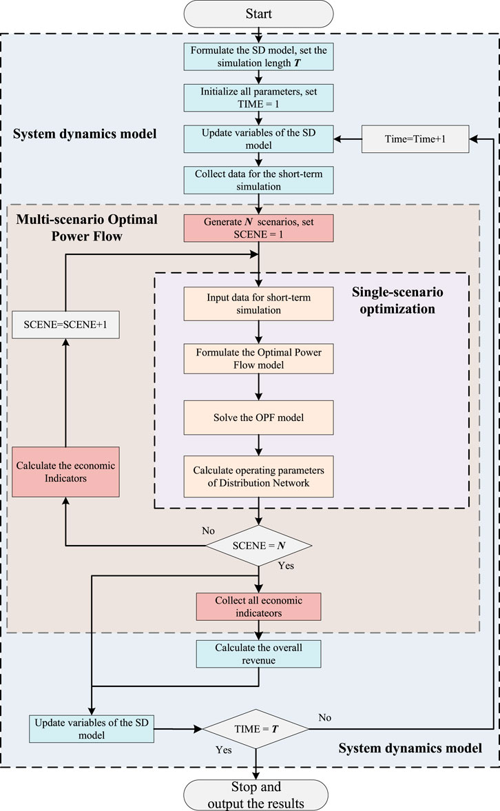
FIGURE 3. Flow chart of the proposed method.

4 Case study

4.1 Scenario setting

In this paper, the IEEE 39-bus system is used for testing. In order to facilitate the calculation of system dynamics model, we set the total load of the IEEE 33-bus system to 600MW, and use the default load of 3.75MW as the benchmark to scale up all load and line parameters in proportion. In the long-term SD simulation, DER increases by a percentage every year, while in the short-term simulation, the newly added capacity of DER is allocated to each node immediately. This paper divides different types of distribution networks to subdivide their respective characteristics and development trends. Combined with the needs of economic and social development for regional distribution network planning, the typical regional characteristics of distribution networks are classified according to the load growth rate and distributed power growth rate, as shown in Table 1.

TABLE 1

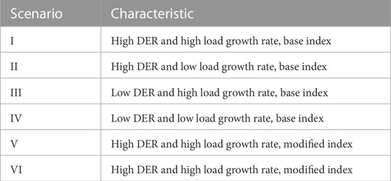
TABLE 1. Different scenarios of the system.

The time period of simulation is 2021–2040 and the time step is 1 year. The parameter setting of exogenous variables are presented in Table 2 where all data are cited from power exchange center (gzp, 2022). It is worth to mention that, since this model only models a certain area, DER Capacity and DESS Capacity from (gzp, 2022) are approximated to meet the needs of this paper.

TABLE 2

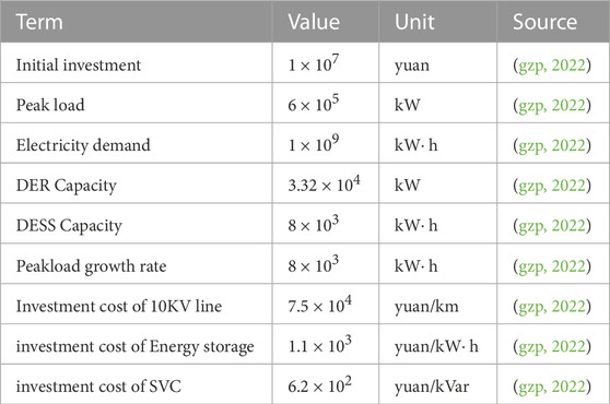
TABLE 2. Parameter setting of the system dynamics model.

4.2 DER trend

First, the long-term trend of DER penetration is shown in the Figure 4. Affected by various factors such as economic conditions, power grid form, and environmental conditions, the four scenarios show great differences. Moreover, a feedback mechanism has been added to the end user sub-model, and the investment in the distribution network has affected the growth of DER, and its trend has reference value. In S1, due to the rapid growth of DER capacity, its power generation also increases rapidly. Therefore, DESS also increases with DER capacity. However, the load growth rate is very high, resulting in a limited increase in the proportion of DER and DESS. In the second scenario, the load does not increase rapidly but the DER increases rapidly, so the electric energy self-sufficiency rate increases significantly. S3 is the opposite, DER grows slowly and load grows fast, resulting in the slowest growth of electric energy self-sufficiency rate. But still reach the 25% level by around 2037. In S4, the load and DER increase slowly, and the electricity self-sufficiency rate is close to Scenario 1. Under the four scenarios, the power self-sufficiency rate is close to S1. The power supply rate at the end of the simulation is between 25%–45%, which highlights the trend of the future distribution network to develop towards a high self-sufficiency rate.

FIGURE 4

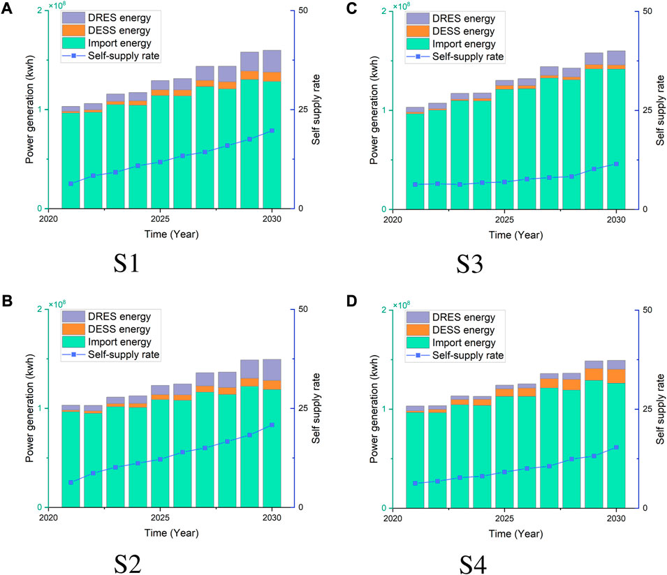
FIGURE 4. Long-term trend of DER penetration.

4.3 Investment analysis

To analyze and maintain various operational indicators within the distribution network under different scenarios, we present the trends of total investment increase and final indicator values in Figure 5. The scenarios demonstrate the varying degrees to which DERs can alleviate the investment pressure on the distribution network, underscoring the significance of strategic DER deployment and planning in achieving a balanced and cost-effective network operation.

FIGURE 5

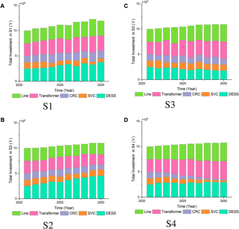
FIGURE 5. Investment ratio adjustment under different scenarios.

Observing Figure 5, it is evident that the total investment in the distribution network exhibits an initial prominent growth trend in S1, followed by a gradual deceleration. This pattern arises due to the substantial increase in load demand necessitating the rapid upgrade of distribution network equipment. Despite the partial offsetting effect of DER on net load, the limited initial DER capacity restricts the potential reduction in investment. Over time, as the cumulative DER capacity reaches a certain threshold, the investment pressure on the distribution network begins to alleviate. In S2, after a slight early-stage increase, the total investment experiences a downward trend, eventually falling below the initial investment amount. This indicates that the rapid growth of DERs has significantly alleviated the operating burden on the distribution network. Conversely, in S3, The rapid growth of load imposes a severe burden on the network, while the scarcity of distributed energy sources reduces the network’s balancing ability. To ensure the stable operation of the system, the investment level of distribution lines and transformers will increase rapidly. Lastly, S4 depicts a slow growth in both load and DERs, resulting in the total investment remaining relatively stable at the initial level, as there’s no urgent need for balancing sources and loads.

According to the growth trend of distributed energy, distribution network investment will also undergo major changes. In S1, the load growth rate is relatively fast, but the proportion of investment in lines and transformers is also gradually increasing. This is because the new power flow of the distribution network brought about by the load growth requires new investment in lines and transformers. Among them, the rapid growth of DESS balances the fluctuation of new energy in the distribution network. In addition, DESS partially replaces the reactive power compensation of SVC and CRC. In S2, investment in line, SVC, and CRC declines, and the proportion of DESS increases rapidly. It shows that the rapid growth of DER requires a large amount of flexible resources, while the rapid growth of DESS partially replaces the role of other investments in the distribution network. Due to the strong volatility and uncertainty of distributed energy sources, which are mostly new energy sources such as wind and solar power, a large amount of DESS is required to cooperate with them to achieve maximum consumption and maintain the safety and stability of the power grid. S3 is the opposite. The small increase of DER leads to the slow growth of DESS, while the increase of load strengthens the demand for lines and other equipment in the distribution network. In S4, due to the small increase in distributed energy and load, the investment ratio is similar to S1, and the investment is concentrated in conventional lines and transformers. Meanwhile, the investment ratios of CRC and SVC are also decreasing year by year. This is because the slow growth of load side and DER does not have high requirements for grid auxiliary services.

4.4 Index structure

This study proposes three distinct types of returns, and their respective proportions in long-term simulations under different scenarios are illustrated in Figure 6. These technical index parameters reflect the real-time performance of the distribution network under different operating conditions and investment scenarios. They are fed as dynamic inputs into the long-term system dynamics model, allowing the investment decisions and revenue forecasts to adapt based on the latest values of these technical parameters. The distribution of benefit types exhibits significant variations among the scenarios. In S1, the higher presence of DER leads to greater environmental benefits. Furthermore, the power quality benefits display an upward trend during long-term operation. This trend can be attributed to the steady growth of DESS investments and loads, which partially enhance the efficacy of reactive power compensation equipment, resulting in increased revenue. In S2, the proportion of direct economic benefits is the highest. This is primarily due to the substantial increase in DER, which leads to a rapid rise in the share of self-supplied power within the distribution network, subsequently driving up revenue from electricity sales. However, as DER enables a significant amount of power consumption within the node, reducing the load on the grid, the demand for reactive power compensation equipment is diminished, thereby reducing its revenue. S3 exhibits the lowest proportion of electricity sales benefits, while power quality and overall benefits are relatively high. This can be attributed to the slower growth of DER, coupled with higher average electricity prices, resulting in lower income from electricity sales. In S4, both DER and DESS experience gradual growth, leading to a more balanced distribution of various benefits across the board.

FIGURE 6

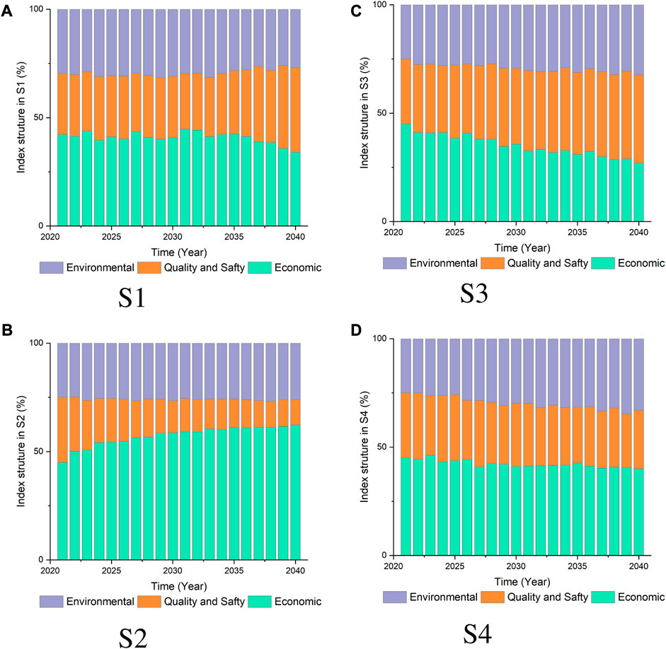
FIGURE 6. Index structure in different scenarios.

4.5 Application of RES and ESS

The utilization of RES and ESS is depicted in Figure 7. In scenarios S1, S2, and S4, curtailment rate of RES is obviously higher. Moreover, the overall curtailment rate of S2 is higher because DER is growing much faster compared to the load, and various adjustment methods cannot achieve real-time power balance, so it can only be partially abandoned for RES. On the contrary, lower loads and DER growth rates reduce system operational risks, improve the matching between the two, and result in a lower curve for S4. In scenarios S1, S2, and S3, the substantial reduction in renewable energy generation results in a high number of hours of energy storage requirement. Conversely, in S4, the slower growth of both load and renewable energy generation leads to a significant increase in the renewable energy penetration rate. Consequently, the demand for energy storage diminishes accordingly.

FIGURE 7

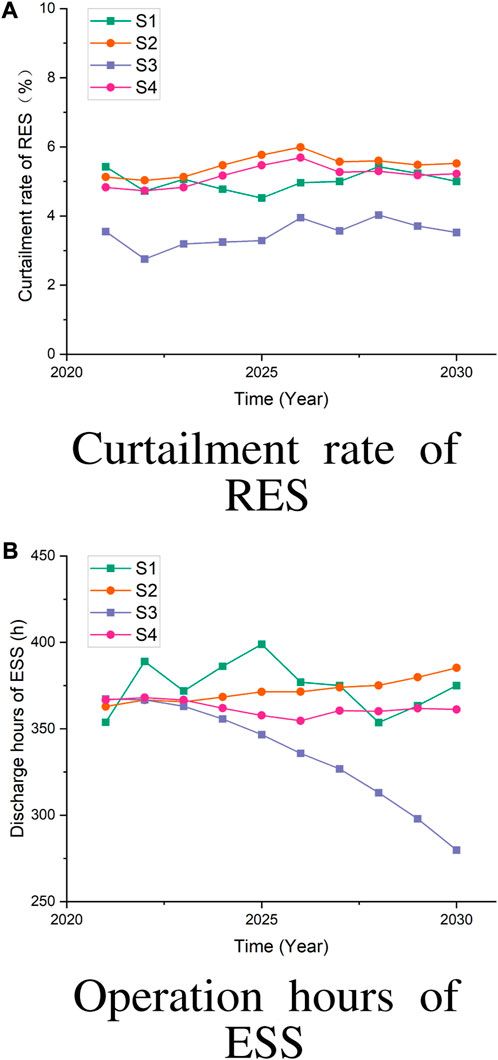
FIGURE 7. Status of RES and ESS in different scenarios.

4.6 The impact of adjusting parameter weights on investment strategy and demand

In this section, a sensitivity analysis is conducted to examine the influence of the adjusted income parameter weight on the model results. S1 will serve as the benchmark case, while new scenarios, S5 and S6, will be designed for comparison. In S5, the weightings assigned to the quality and safety index, environmental index, and economic index are 0.3, 0.3, and 0.4, respectively. Conversely, in S6, the weightings assigned to the quality and safety index, environmental index, and economic index are 0.2, 0.4, and 0.4, respectively. The results are shown in Figure 8; Figure 9.

FIGURE 8

FIGURE 8. Index structure in different scenarios.

FIGURE 9

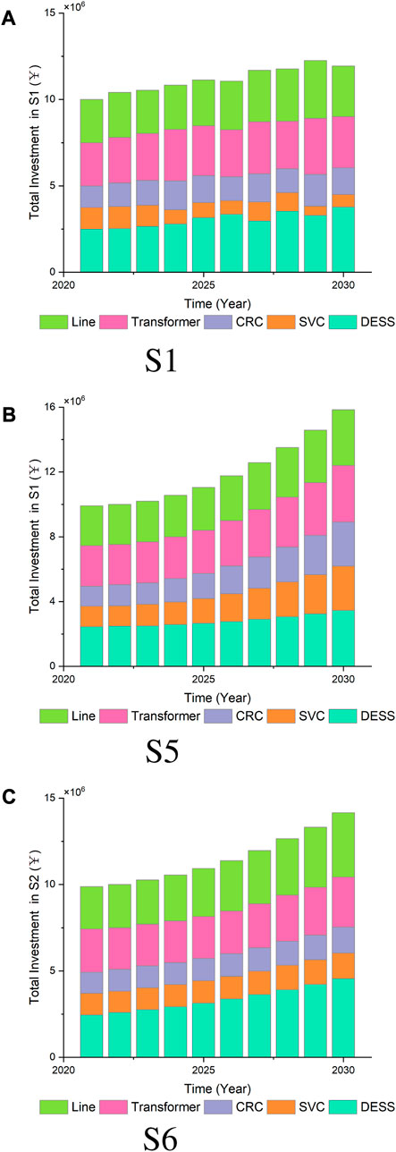
FIGURE 9. Investment adjustment in different scenarios.

It is evident that both environmental indicators, namely, energy self-sufficiency and the integration rate of renewable energy, exhibit substantial proportions in both S5 and S6. Conversely, the proportions of quality and safety indicators display a decreasing trend. This trend can be attributed to the significant environmental benefits brought about by the expansion of DER, which consequently yields a relatively higher return on investment in this aspect. In contrast, the growing installed capacity of DERs ensures the power supply capacity and reliability of the distribution network, leading to relatively lower investment benefits in terms of quality and safety indicators. Meanwhile, the total investment shows a rapid growth trend in both S5 and S6. This is partly due to the decline of the economic index, which makes the investor tend to invest more funds to achieve the construction of distributed energy system. Meanwhile, in S6, it can be noticed that growth rate of investment in DESS is significantly faster, while its transmission line investment is relatively slow. This may be caused by its high environmental index and low safety index.

4.7 Sensitivity analysis of DER capacity

A sensitivity analysis is conducted to examine the influence of Total Investment, Peak Load Growth Rate and Demand Growth Rate on DER capacity. The result is shown in Figure 10. Figure 10B shows that peak load growth rate has little impact on DER capacity. This is because DER is mostly made of new energy sources such as wind and solar, which itself has great volatility and uncertainty, making it difficult to effectively support peak load demand. Therefore, there is little coupling between DER capacity and peak load growth rate. On the contrary, changes in aggregate demand will significantly affect the development of DER capacity, as shown in the Figure 10A. This is because in the future, DER will be one of the important energy sources and play a decisive role in the total load demand. Therefore, the acceleration of load growth rate will significantly stimulate the development of DER. The impact of total investment on DER capacity is less than that of demand growth, as shown in Figure 10C. This is because the investment amount needs to increase exponentially if it wishes to achieve higher investment benefits in some other investment areas of the power system, such as grid capacity transformation and transformer capacity transformation, leaving Not much for DER.

FIGURE 10

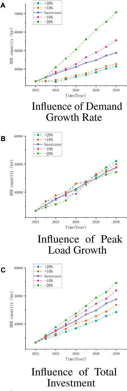
FIGURE 10. Sensitivity analysis of DER capacity.

5 Conclusion

The growth of distributed generation brings new challenges to distribution network planning. Traditional planning methods fail to effectively divide the indicators for the multi-objective characteristics of distribution network investment. And it is unable to take into account the changes of other related elements under the long-term scale to realize the shortcoming of dynamic adjustment. This paper integrates simulations of system dynamics and optimal power flow models at two different time scales. In the long-term simulation, a multi-objective and multi-element complex system is constructed, and in the short-term simulation, the basic constraints of the distribution network are verified. The obtained simulation results are more convincing. The results show that in the distribution network with different development conditions, the income of each investment is different, and the distribution of investment should also be adjusted according to the characteristics of the distribution network. Overall, in the high DER and low load growth rate scenario, investment demand for various aspects of the power grid will increase synchronously, and the most important indicator of the power grid will gradually become the quality and safety of the grid. This is also the most likely situation that China may face. In this scenario, it is very important to coordinate and plan investment projects for the healthy, safe, and stable operation of the power grid.

The long-term simulation model studied in this paper does not consider the impact of the electricity market. In the future, distributed energy will enter the wholesale power market through aggregation, or end-user peer-to-peer transactions will become the mainstream trend. The short-term simulation only studies the optimal power flow problem, focusing on the scheduling of conventional scenarios, while ignoring some extreme scenarios and fault analysis. And the model does not accurately model some parameters with uncertainties in the distribution network operation. In the future, starting from these three points, we will further analyze the impact of the power market, fault scenarios and uncertainties on the simulation.

Data availability statement

The original contributions presented in the study are included in the article/Supplementary Material, further inquiries can be directed to the corresponding author.

Author contributions

QL: Conceptualization, Data curation, Funding acquisition, Methodology, Project administration, Resources, Software, Visualization, Writing–original draft, Writing–review and editing. YL: Data curation, Funding acquisition, Investigation, Methodology, Software, Software, Writing–review and editing.

Funding

The author(s) declare that no financial support was received for the research, authorship, and/or publication of this article. This work was supported in part by the State Grid Hubei Electric Power Company under Grant 22H0455. The funder was not involved in the study design, collection, analysis, interpretation of data, the writing of this article, or the decision to submit it for publication.

Conflict of interest

Author QL was empolyed by State Grid Corporation of China.

The authors declare that this study received funding from State Grid Hubei Electric Power Company. The funder was not involved in the study design, collection, analysis, interpretation of data, the writing of this article, or the decision to submit it for publication.

Publisher’s note

All claims expressed in this article are solely those of the authors and do not necessarily represent those of their affiliated organizations, or those of the publisher, the editors and the reviewers. Any product that may be evaluated in this article, or claim that may be made by its manufacturer, is not guaranteed or endorsed by the publisher.

References

Adefarati, T., and Bansal, R. C. (2019). Reliability, economic and environmental analysis of a microgrid system in the presence of renewable energy resources. Appl. energy 236, 1089–1114. doi:10.1016/j.apenergy.2018.12.050

CrossRef Full Text | Google Scholar

Chi, Y.-y., Zhao, H., Hu, Y., Yuan, Y.-k., and Pang, Y.-x. (2022). The impact of allocation methods on carbon emission trading under electricity marketization reform in China: A system dynamics analysis. Energy 259, 125034. doi:10.1016/j.energy.2022.125034

CrossRef Full Text | Google Scholar

Cui, Q., Bai, X., and Dong, W. (2019). Collaborative planning of distributed wind power generation and distribution network with large-scale heat pumps. CSEE J. Power Energy Syst. 5, 335–347. doi:10.17775/CSEEJPES.2019.00140

CrossRef Full Text | Google Scholar

Dhivya, S., and Arul, R. (2021). Demand side management studies on distributed energy resources: A survey. Trans. Energy Syst. Eng. Appl. 2, 17–31. doi:10.32397/tesea.vol2.n1.2

CrossRef Full Text | Google Scholar

Ehsan, A., and Yang, Q. (2019). State-of-the-art techniques for modelling of uncertainties in active distribution network planning: A review. Appl. energy 239, 1509–1523. doi:10.1016/j.apenergy.2019.01.211

CrossRef Full Text | Google Scholar

Guangzhou Power Exchange Center (2022). Available at: https://www.gzpec.cn/main/index.do.

International Energy Agency (2022). Unlocking the potential of distributed energy resources. Paris: International Energy Agency.

Google Scholar

Li, J., Luo, Y., and Wei, S. (2022). Long-term electricity consumption forecasting method based on system dynamics under the carbon-neutral target. Energy 244, 122572. doi:10.1016/j.energy.2021.122572

CrossRef Full Text | Google Scholar

Luo, L., Abdulkareem, S. S., Rezvani, A., Miveh, M. R., Samad, S., Aljojo, N., et al. (2020). Optimal scheduling of a renewable based microgrid considering photovoltaic system and battery energy storage under uncertainty. J. Energy Storage 28, 101306. doi:10.1016/j.est.2020.101306

CrossRef Full Text | Google Scholar

Maheshwari, A., Heleno, M., and Ludkovski, M. (2020). The effect of rate design on power distribution reliability considering adoption of distributed energy resources. Appl. energy 268, 114964. doi:10.1016/j.apenergy.2020.114964

CrossRef Full Text | Google Scholar

Panigrahi, R., Mishra, S. K., Srivastava, S. C., Srivastava, A. K., and Schulz, N. N. (2020). Grid integration of small-scale photovoltaic systems in secondary distribution network—A review. IEEE Trans. Industry Appl. 56, 3178–3195. doi:10.1109/tia.2020.2979789

CrossRef Full Text | Google Scholar

Song, X.-h., Han, J.-j., Zhang, L., Zhao, C.-p., Wang, P., Liu, X.-y., et al. (2021). Impacts of renewable portfolio standards on multi-market coupling trading of renewable energy in China: A scenario-based system dynamics model. Energy Policy 159, 112647. doi:10.1016/j.enpol.2021.112647

CrossRef Full Text | Google Scholar

Tang, L., Guo, J., Zhao, B., Wang, X., Shao, C., and Wang, Y. (2021). Power generation mix evolution based on rolling horizon optimal approach: A system dynamics analysis. Energy 224, 120075. doi:10.1016/j.energy.2021.120075

CrossRef Full Text | Google Scholar

Teufel, F., Miller, M., Genoese, M., and Fichtner, W. (2013). Review of system dynamics models for electricity market simulations.

Google Scholar

Thang, V. (2021). Optimal sizing of distributed energy resources and battery energy storage system in planning of islanded micro-grids based on life cycle cost. Energy Syst. 12, 637–656. doi:10.1007/s12667-020-00384-x

CrossRef Full Text | Google Scholar

Yi, Z., Xu, Y., Gu, W., Yang, L., and Sun, H. (2021). Aggregate operation model for numerous small-capacity distributed energy resources considering uncertainty. IEEE Trans. Smart Grid 12, 4208–4224. doi:10.1109/tsg.2021.3085885

CrossRef Full Text | Google Scholar

Ying, Z., Xin-gang, Z., and Zhen, W. (2020). Demand side incentive under renewable portfolio standards: A system dynamics analysis. Energy Policy 144, 111652. doi:10.1016/j.enpol.2020.111652

CrossRef Full Text | Google Scholar