Numerical analysis of thermoelectric power generation coupled with temperature-dependent material properties

1 Introduction

Thermoelectric generator (TEG), owning to its solid-state energy conversion characteristic, is a potential power supply and energy harvesting technology in the fields of space exploration (Liu et al., 2020), waste heat recovery (Shen et al., 2019), emergency power generation (Li et al., 2021), wearable electronics (Nozariasbmarz et al., 2020), portable power sources (Li et al., 2020a), smart buildings (Lin et al., 2022), and solar utilization (Lv et al., 2019). The inherent advantage of the sold-state energy conversion characteristic is endowed by the Seebeck effect, which expounds the driving force of electrons inside metals or semiconductors by temperature difference. Nowadays, extensive and intensive studies are constantly emerging from material (Hinterleitner et al., 2019) to device (Pourkiaei et al., 2019) and then to system (Alghoul et al., 2018) levels.

In the device level, the thermal–electrical multi-physics of the thermoelectric module (TEM) during power generation must be fully understood in order to develop high performance TEG systems. The thermal–electrical multi-physics governs the working process of a TEG system, which acts as a bridge between the thermoelectric (TE) material and TEG system. However, the TEM thermal–electrical multi-physics is extraordinarily complicated and results in compromised assumptions in lots of existing studies. An ordinary assumption is of its constant material properties (thermal conductivity, Seebeck coefficient, and electrical resistivity) so as to obtain a mathematical solution of the energy equation (Rowe, 1995). In one-dimensional framework, the constant material property assumption directs the temperature profile along the TE leg to be parabolic (Rowe and Gao, 1998). However, TE material properties are temperature dependent and are subjected to considerable variations (Sun et al., 2019). The thermal–electrical multi-physics inside a TEM when coupled with temperature-dependent material properties has not been fully understood and has attracted attention recently. A brief literature review is presented in the following paragraph.

Fraisse et al. (2013) compared different simplified models without considering temperature-dependent material properties. The results found that the one-dimensional model was accurate enough. However, several studies have found that the Thomson effect induced by temperature-dependent material properties causes considerable influence on TEG performance. Wee (2011) concluded that the Thomson effect is essential to understand the TE efficiency qualitatively and quantitatively. Manikandan and Kaushik (2016) found that the Thomson effect decreases the maximum power output and efficiency. Hereafter, further studies were devoted to reveal the influence of temperature-dependent material properties on TEG performance. Wee (2018) proposed a technique of polynomial chaos expansion to quantify the uncertainty and sensitivity of TEG performance due to temperature-dependent material properties. In order to avoid the difficulty of obtaining the analytical solution of the temperature profile, Lee et al. (2018) used third-order polynomial temperature-dependent material properties to calculate the effective material properties. An outstanding study conducted by Ju et al. (2017) proposed an approximate analytical model to obtain the solution of one-dimensional energy equation with second-order temperature-dependent material properties. The essential idea is to assume a linear temperature profile to calculate electrical resistivity and the Thomson coefficient, while the thermal conductivity is coupled during the derivation of the temperature profile. Cui et al. (2019) employed the homotopy perturbation method and finite difference scheme to solve the strong non-linear thermal-electric stress–coupled energy equation. Their results revealed that the criterion to assess TEG performance becomes complex when temperature-dependent material properties are taken into consideration. Ponnusamy et al. (2020) performed a detailed study on TEG performance discrepancy between constant and temperature-dependent material properties. The results indicated that the deviation was caused by the asymmetric distribution of Joule heat and internally released Thomson heat along the TE leg. There are several numerical studies on TEG. For example, Eldesoukey and Hassan (2019) adopted Fluent to predict the power generation characteristic in a three-dimensional framework, and Sun et al. (2022) and Luo et al. (2023) developed a three-dimensional transient numerical model to investigate the heat recovery potential with TEG technology. The abovementioned three-dimensional numerical studies on TEG focused on the macroscopic performance of the TEG, while the influence of temperature-dependent material properties on the temperature distribution and the heat flux profile inside the TE leg have not yet been investigated.

Surveying the abovementioned studies concerning the influence of temperature-dependent material properties on TEG performance, few studies have presented the temperature and heat flux profile inside the TE leg (Ju et al., 2017) even under the one-dimensional framework because the energy equation considering the temperature-dependent material properties becomes unsolvable with the ordinary analytical tool. TE material properties are sensitive to temperature; for example, the first-order or second-order polynomial temperature-dependent material properties of Te₂Bi₃-based TEM are not accurate enough (Lee et al., 2018).

The difficulty in solving the energy equation when considering temperature-dependent material properties is mainly caused by the following contradiction: accurate thermal conductivity, Seebeck coefficient, and electrical resistivity are required to solve the temperature profile, but these accurate properties cannot be obtained before the provision of the temperature profile. The abovementioned situation indicates that a mathematically complete solution cannot be obtained. A straightforward method is to first find out an “entry point” from the energy equation and then employ the iteration method to complete the rounding problem of the energy equation. To the best of the authors’ knowledge, the abovementioned idea has not been tried in previous studies, and the present work performs an initial attempt. Concerning the “entry point” of the energy equation, the calculation of the internal electrical resistance is worth trying because the generated current can be obtained once the internal electrical resistance is provided. Hence, the remaining problem is to return back the obtained temperature profiles for the calculation of internal electrical resistance until the difference of internal electrical resistance is small enough during two iterations. The abovementioned idea requires no further assumptions on how many orders of temperature-dependent material properties, which implies that the Seebeck, Joule, Peltier, and Thomson effects can be comprehensively considered and coupled with accurate temperature-dependent material properties. In general, third-order polynomial temperature-dependent material properties are accurate enough and technically sound.

In this work, a one-dimensional numerical model for TEG optimization is proposed, which couples with third-order polynomial temperature-dependent material properties (thermal conductivity, Seebeck coefficient, and electrical resistivity) so as to include all the necessary effects, namely, the Seebeck, Joule, Peltier, and Thomson effects. An efficient numerical method is developed to solve the inter-coupling energy equation. The abovementioned numerical model, which is not reported in previous studies, is featured by comprehensive consideration of all TE effects, fast convergence, low demand of computation resource, and program simplicity. The temperature and heat flux distributions along the TE leg, electric power output, TE efficiency, and Thomson influence under different external loads are investigated in detail. The influence of temperature-dependent material properties on temperature distribution, insights of the temperature and heat flux responses when modifying external loads, and structural optimization potential of TEM aiming to augment TE efficiency are focused and comprehensively discussed. The present work provides an efficient and comprehensive one-dimensional numerical model to predict TEG performance and also contributes to the justification of the assumption of constant material properties in previous studies.

2 Methodology

2.1 TEM model

The TEM model is illustrated in Figure 1. The hot/cold substrates and copper pads are required to manufacture the TEM, yet only the TE legs are considered in the present work. This implies that thermal resistances caused by substrates and copper pads, thermal/electrical contacts, and convective/radiative thermal leaks inside the TEM are not considered. The abovementioned source terms, which are thermal resistances/contacts and various thermal leaks, can be conveniently incorporated. The present work focuses on solving the highly non-linear energy equation when considering temperature-dependent material properties. Note that the generated current results in further heat pumping from the hot-end to the cold-end when the TEM is subjected to the power generation mode. This is confirmed in various experiments (Li et al., 2019). The z-coordinate in Figure 1B starts from the cold-end of the TE leg and directs to the hot-end.

FIGURE 1

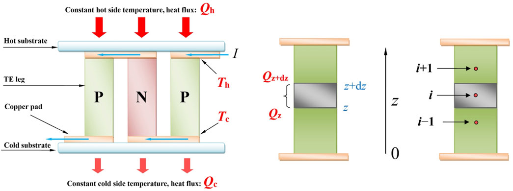
FIGURE 1. TEM model in the power generation mode and coordinate system.

2.2 Governing equation

The governing energy equation for the TE leg can be derived on the basis of energy conservation, the first Thomson relation and second Thomson relation. The governing energy equation can be expressed as follows after treating the current (I) as scalar.

$\frac{d\left(-k\left(T\right)\cdot \frac{dT}{dz}\right)}{dz}=\frac{I^2\rho }{A^2}\pm \frac{\left|I\right|}{A}T\frac{d\alpha }{dT}\frac{dT}{dz},(1)$

where + is for P-type leg and − is for N-type leg. Note that this governing equation is consistent with previous references (Ju et al., 2017; Lee et al., 2018). This partial equation can be solved under the assumption that the properties (α, ρ, and k) of the TE material are independent of the temperature. The obtained result is as follows:

$T=-\frac{I^2\rho }{2k{A}^2}{z}^2+\left(\frac{T_h-T_c}{L}+\frac{I^2\rho L}{2k{A}^2}\right)z+T_c,(2)$

where T_h, T_c, L, and A are the hot-end temperature, cold-end temperature, length of the TE leg, and cross-sectional area of the TE leg, respectively. The temperature distribution along the TE leg is parabolic on the basis of Eq. 2. Therefore, Eq. 2 is referred to as the second-order temperature distribution. In case that temperature-dependent material properties are considered, the temperature distribution should be more complex.

2.3 Material property

Bi₂Te₃-based TE material is used widely and can be obtained easily in the open market. Therefore, temperature-dependent material properties of the Bi₂Te₃-based TE material from Sagreon Co., Ltd., China, are used in the present work. However, the proposed model is not limited to the Bi₂Te₃-based TE material. Third-order polynomial fittings are applied (Li et al., 2020b) as follows:

$k_p\left(T\right)=t{p}_1+t{p}_{2}T+t{p}_3{T}^2+t{p}_4{T}^3,(\mathrm{3-1})$

$k_n\left(T\right)=t{n}_1+t{n}_{2}T+t{n}_3{T}^2+t{n}_4{T}^3,(\mathrm{3-2})$

${\rho }_p\left(T\right)=e{p}_1+e{p}_{2}T+e{p}_3{T}^2+e{p}_4{T}^3,(\mathrm{4-1})$

${\rho }_n\left(T\right)=e{n}_1+e{n}_{2}T+e{n}_3{T}^2+e{n}_4{T}^3,(\mathrm{4-2})$

${\alpha }_p\left(T\right)=s{p}_1+s{p}_{2}T+s{p}_3{T}^2+s{p}_4{T}^3,(\mathrm{5-1})$

${\alpha }_n\left(T\right)=s{n}_1+s{n}_{2}T+s{n}_3{T}^2+s{n}_4{T}^3.(\mathrm{5-2})$

The constants in Eqs 3–5 are as follows:

$t{p}_1=4.389,t{p}_2=-1.8168✕{10}^{-2},t{p}_3=2.437956✕{10}^{-5},t{p}_4=4.793196✕{10}^{-10},$

$t{n}_1=4.09878,t{n}_2=-1.4976✕{10}^{-2},t{n}_3=1.799196✕{10}^{-5},t{n}_4=1.692996✕{10}^{-9},$

$e{p}_1=-6.7074✕{10}^{-6},e{p}_2=5.09✕{10}^{-8},e{p}_3=6.33243✕{10}^{-11},e{p}_4=-5.31761✕{10}^{-14},$

$e{n}_1=-1.51744✕{10}^{-5},e{n}_2=1.142✕{10}^{-7},e{n}_3=-8.17056✕{10}^{-11},e{n}_4=-5.18487✕{10}^{-15},$

$s{p}_1=-1.0915819✕{10}^{-4},s{p}_2=1.67585✕{10}^{-6},s{p}_3=-2.12✕{10}^{-9},s{p}_4=4.43743✕{10}^{-14},$

$s{n}_1=-4.3833365✕{10}^{-4},s{n}_2=2.90422✕{10}^{-6},s{n}_3=-9.76✕{10}^{-9},s{n}_4=1.01202✕{10}^{-11}.$

2.4 Mathematical model

For a control volume (CVM) of AΔz (Δz is the length of the control volume), number the control volume from the cold-end to the hot-end, and the first control volume has two nodes, i.e., i = 0 and i = 1. An algorithm to calculate the temperature of the (i+1)^th control volume can be derived on the basis of energy conservation and Eq. 1 as follows:

$\begin{array}{l}k\left(T\left[i\right]\right)A\frac{T\left[i\right]-T\left[i-1\right]}{\Delta z}=\\ k\left(T\left[i\right]\right)A\frac{T\left[i+1\right]-T\left[i\right]}{\Delta z}+\frac{I^2\rho \left(T\left[i\right]\right)\Delta z}{A}\pm \mu \left(T\left[i\right]\right)\frac{\left|I\right|}{A}\frac{T\left[i+1\right]-T\left[i-1\right]}{2\Delta z}A\Delta z,\end{array}(6)$

Note that the (i + 1)^th control volume is physically realistic. Such numbering rules avoid the confusing zero control volume, and it is beneficial during coding. The second and third terms in the right-hand side of Eq. 6 represent the Joule heat and Thomson heat, respectively. + is for P-type TE leg and − is for N-type TE leg. As a result, Eq. 6 can be combined to obtain the temperature distribution along the TE leg based on the CVM as follows:

$T\left[i\right]=0.5\left(T\left[i-1\right]+T\left[i+1\right]\right)+\frac{I^2\rho \left(T\left[i\right]\right)\Delta z^2}{2k\left(T\left[i\right]\right)A^2}\pm \mu \left(T\left[i\right]\right)\frac{\left|I\right|\Delta z}{4k\left(T\left[i\right]\right)A}\left(T\left[i+1\right]-T\left[i-1\right]\right)(7)$

On the other hand, by applying a second-order central finite difference algorithm on Eq. 1, the following algorithm can be derived to obtain the temperature distribution based on the finite difference method (FDM) as follows:

$\begin{array}{l}T\left[i\right]=0.5\left(T\left[i-1\right]+T\left[i+1\right]\right)+\frac{I^2\rho \left(T\left[i\right]\right)\Delta z^2}{2k\left(T\left[i\right]\right)A^2}\pm \mu \left(T\left[i\right]\right)\frac{\left|I\right|\Delta z}{4k\left(T\left[i\right]\right)A}\left(T\left[i+1\right]-T\left[i-1\right]\right)\\ +\frac{k_d\left(T\left[i\right]\right)}{8k\left(T\left[i\right]\right)}\left(T^2\left[i+1\right]+T^2\left[i-1\right]-2T\left[i+1\right]T\left[i-1\right]\right)\end{array}(8)$

where + is for P-type TE leg and − is for N-type TE leg. k_d is the first-order derivative of k. By comparing Eqs 7 and 8, these two numerical models were found to be the same, except for the fourth term in the right-hand side of Eq. 8. This term represents the influence of the local change rate of thermal conductivity on temperature distribution, whereas the thermal conductivity inside a CVM is assumed to be unchanged.

The electric current and internal electrical resistances are coupled with the temperature distribution. As a consequence, Eqs 7 and 8 become difficult to be solved. An iteration method is required to decouple the abovementioned problem. The open circuit voltage can be obtained as follows:

$\begin{array}{l}{V}_{OC}=N{\int }_{T_c}^{T_h}\left({\alpha }_P-{\alpha }_N\right)dT\\ =N\left[sp{n}_1\left(T_h-T_c\right)+\frac{1}{2}sp{n}_2\left({T_h}^2-{T_c}^2\right)+\frac{1}{3}sp{n}_3\left({T_h}^3-{T_c}^3\right)+\frac{1}{4}sp{n}_4\left({T_h}^4-{T_c}^4\right)]\right.,\end{array}(9)$

where spn₁ = sp₁ − sn₁, spn₂ = sp₂ − sn₂, spn₃ = sp₃ − sn₃, and spn₄ = sp₄ − sn₄. The internal electrical resistance cannot be obtained because the temperature distribution is not known. However, the averaged internal electrical resistance can be used as an initial value to decouple Eqs 7 and 8 as follows:

$R_{in}=\frac{N}{A}{\int }_0^L\left({\rho }_p+{\rho }_n\right)dz=\frac{N}{A}\left({\rho }_{Pav}+{\rho }_{Nav}\right)L,(10)$

where N is the number of TE couples inside the TEM. The average electrical resistivity can be determined based on Eq. 4 as follows:

$\begin{array}{l}{\rho }_{Pav}=\frac{1}{T_h-T_c}{\int }_{T_c}^{T_h}{\rho }_p\left(T\right)dT\\ =\frac{1}{T_h-T_c}\left[e{p}_1\left(T_h-T_c\right)+\frac{1}{2}e{p}_2\left({T_h}^2-{T_c}^2\right)+\frac{1}{3}e{p}_3\left({T_h}^3-{T_c}^3\right)+\frac{1}{4}e{p}_4\left({T_h}^4-{T_c}^4\right)]\right.,\end{array}(\mathrm{11-1})$

$\begin{array}{l}{\rho }_{Nav}=\frac{1}{T_h-T_c}{{\int }_{T_c}^{T_h}\rho }_n\left(T\right)dT\\ =\frac{1}{T_h-T_c}\left[e{n}_1\left(T_h-T_c\right)+\frac{1}{2}e{n}_2\left({T_h}^2-{T_c}^2\right)+\frac{1}{3}e{n}_3\left({T_h}^3-{T_c}^3\right)+\frac{1}{4}e{n}_4\left({T_h}^4-{T_c}^4\right)]\right.,\end{array}(\mathrm{11-2})$

Hence, the electric current can be determined when the external load (R_ex) is provided as follows:

$I=\frac{V_{OC}}{R_{in\text{av}}+R_{\text{ex}}},(12)$

The TE efficiency is obtained when R_ex = R_in and is defined as follows:

$\zeta =\frac{P_{\max }}{Q_h}=\frac{V_{OC}^2}{Q_h{R}_{in}},(13)$

where Q_h is the heat flow from the hot-end of the TEM, and it is calculated as follows:

$Q_{\mathrm{h}}=N\left[-k_P\left(T_{\mathrm{h},\mathrm{P}}\right){\left.A\frac{d{T}_{\mathrm{P}}}{dz}\right|}_{z=L}+{\alpha }_{\mathrm{P}}\left(T_{\mathrm{h},\mathrm{P}}\right)I{T}_{\mathrm{h},\mathrm{P}}-k_{\mathrm{N}}\left(T_{\mathrm{h},\mathrm{N}}\right){\left.A\frac{d{T}_{\mathrm{N}}}{dz}\right|}_{z=L}+{\alpha }_{\mathrm{N}}\left(T_{\mathrm{h},\mathrm{N}}\right)I{T}_{\mathrm{h},\mathrm{N}}]\right.(14)$

Boundary conditions, which are T = T_c at z = 0 m and T = T_h at z = L m have to be employed in the numerical model. Note that only constant temperature conditions are employed in the present study because most of the previous studies on TEG have applied this type of boundary condition. For the constant heat flux boundary condition, a recent insightful investigation has reported observations in detail (Min, 2022). Eqs 2–14 were coded with C language to explore the influence of temperature-dependent material properties on TEG performance and to find out the underlying thermal–electrical multi-physics during TE conversion.

2.5 Closing the rounding problem of internal electrical resistance

As stated previously, the averaged internal electrical resistance is used as an initial value to decouple Eqs 7 and 8. Then, the new internal electrical resistance must be re-calculated once the temperature distribution is obtained. Hereby, iterations have to be performed to obtain new temperature distributions until the internal electrical resistance between two iterations becomes small enough (e.g., 0.0001 Ω). In general, several iterations (less than five iterations) are enough. This also implies that a satisfied temperature distribution is obtained. The CPU time for each set of input parameters (a, L, F, T_h, T_c, and R_ex) is 3.82 s with a 12th Intel i7-1260P processor, and the total CPU time for structure optimization depends on the number of parameter sets. Figure 2 shows the flow chart of the developed numerical model. Note that another subroutine is required to obtain the leg temperature distribution, T_P (z) and T_N (z) in subroutine B. Hence, there are three different levels of the loop program. An ordinary least squares method was used to obtain T_P (z) and T_N (z), and this subroutine is not shown for the sake of briefness.

FIGURE 2

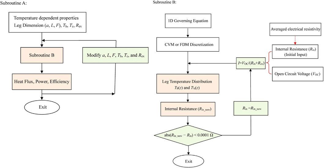
FIGURE 2. Flow chart of the developed numerical model considering temperature-dependent properties.

3 Results and discussions

3.1 Model verification

Figure 3 shows the experimental setup for the verification of the developed numerical model. The tested TEM is a commercially available TEG1-12708 from Sagreon Co., Ltd., China. The dimensions are 40 mm × 40 mm × 3.8 mm, and the temperature-dependent properties can be found in our previous work (Li et al., 2020b). In order to obtain a constant hot-end temperature, high temperature silicon oil with a boiling temperature of 573 K was used to transfer heat from the electrical heater to the copper-based heat collector and distributor. The hot-end temperature was set with a temperature controller. The cold-end temperature was ensured with an alumina heat sink, a blower, and a speed controller. Thermal grease and a weight of 10 kg were applied to decrease the thermal contacts between the TEM and heat-distributor/heat-sink. The generated power was measured with an electronic load (Prodigit 3311F) by adjusting different external loads. The accuracy of the electronic load was ±0.5%. Two thermocouples with diameters of 0.5 mm were carefully installed in the pre-grooved heat-distributor/heat-sink. The accuracy of the thermocouple was ±0.5%. All experimental cases were run at least 2 h before performing measurements so as to eliminate possible unsteady conditions. The cold-end temperature was maintained at 323 K by adjusting the blower speed. The cold-end temperature of 323 K was necessary for forced air cooling because a certain temperature difference between the cold-end temperature and atmospheric temperature is required. The atmospheric temperature during the experiments was 299 K.

FIGURE 3

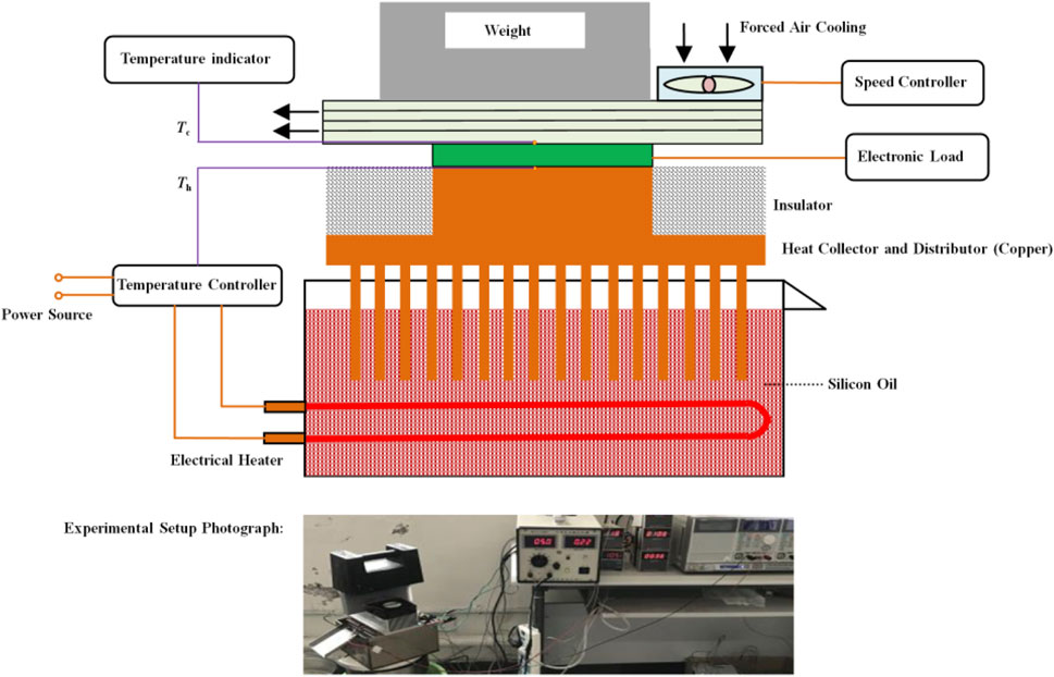
FIGURE 3. Experimental setup for verification of the developed numerical model.

As shown in Figure 4, the predicted results agree well with the experimental data under the same hot-/cold-end temperatures. The average experimental electric powers are 0.023 W, 0.107 W, 0.238 W, and 0.412 W lower than that obtained by the developed numerical model under the hot-end temperatures of 373 K, 423 K, 473 K, and 523 K, respectively. The reasons for the error include the negligence of thermal/electrical contacts and the one-dimensional assumption of the TE leg. For example, the effective temperature difference is lower than that in the numerical model, which leads to less electric power than that by the numerical model. Hence, the developed numerical model can predict the TEG performance with acceptable errors. Furthermore, the developed numerical model can be used to reveal various aspects of the underlying thermal–electrical multi-physics as given in the following sections.

FIGURE 4

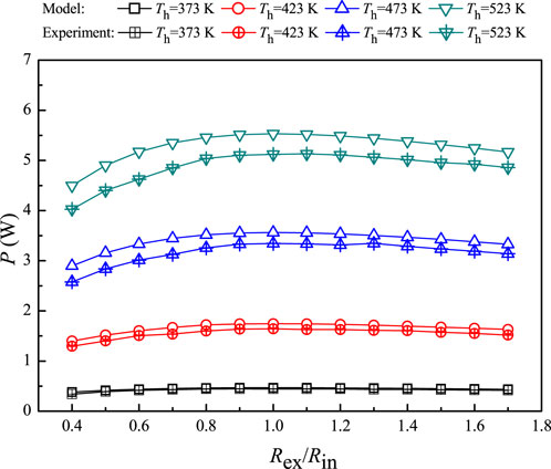
FIGURE 4. Comparisons between the predicted results and experimental data under various hot-end temperatures under the cold-end temperature of 323 K.

3.2 Comparison between CVM and FDM

Figure 5 shows the comparisons on the convergent performance between the CVM and FDM in obtaining T_P (z) and T_N (z) in subroutine B. In order to present the convergent process, T_p − T_2nd is used as the monitor parameter. As shown in Figure 5, the FDM performs much better than the CVM, that is, the FDM is found to have converged much faster with fewer grids than the CVM. For the FDM, it usually takes several seconds to reach satisfied solutions of T_P (z) and T_N (z). Note that the maximum T_p − T_2nd is found to be approximately 0.5 K when the CVM is employed, yet the corresponding value is approximately 1.3 K for the FDM. The underlying reason for the abovementioned phenomenon is the inclusion of the local change rate of thermal conductivity in the FDM, that is, the fourth term in the right-hand side of Eq. 8. This reveals that the local change rate of thermal conductivity considerably affects the temperature distribution. In fact, the thermal conductivity is of more priority than the Seebeck coefficient and electrical resistivity during the optimization of TEG performance (Shen et al., 2021). Hence, the local change rate of thermal conductivity inevitably affects the temperature distribution.

FIGURE 5

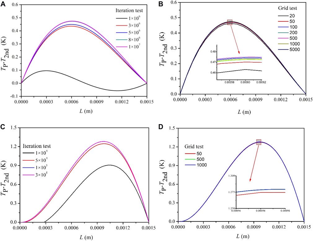
FIGURE 5. Comparisons on convergent performance between CVM and FDM (T_h = 443 K and T_c = 323 K). (A) Iteration test of CVM. (B) Grid test of CVM. (C) Iteration test of FDM. (D) Grid test of FDM.

Figure 6 presents the temperature difference for P-/N-type legs with different numerical methods. As shown in Figure 6, the maximum temperature differences between the FDM and CVM can be as large as 1.0 K, but the locations for the abovementioned maximum temperature difference are different. For the P-type leg, the abovementioned location is near the hot-end of TEM, whereas it is near the cold-end of TEM for the N-type leg. To the best of the authors’ knowledge, this phenomenon has not been reported in previous studies, yet our experiments cannot confirm this finding due to the limitation of measurement techniques. Further theoretical studies and advanced experiments have to be carried out to verify this finding. Therefore, the temperature distributions for the P-/N-type legs are found to be different, which are presented and discussed in detail in the following section. In the following sections, all results are obtained on the basis of the FDM.

FIGURE 6

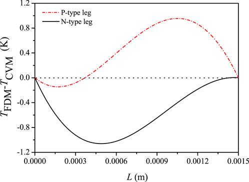
FIGURE 6. Comparisons of results between CVM and FDM (T_h = 443 K and T_c = 323 K).

3.3 Temperature distribution

Figure 7 presents the temperature distribution of the P-/N-type legs when compared to the linear and parabolic temperature distributions. A well-accepted conclusion for the second-order temperature distribution is that the location of the maximum temperature difference is at the central point of the leg (Rowe and Gao, 1998). However, temperature distributions considering temperature-dependent material properties are inconsistent with the second-order temperature distribution. The temperature of the P-type leg is always larger than that predicted by the second-order temperature distribution in every location of the leg, whereas the temperature of the N-type leg is always lower than that predicted by the second-order temperature distribution. The maximum temperature difference for the P-type leg is approximately 2.2 K when compared to that of linear temperature distribution, whereas the corresponding value is approximately 0.9 K for the second-order temperature distribution. Moreover, the location of the maximum temperature difference for the P-type leg is not at the central point of the leg. The abovementioned finding answers the doubt of the influence degree of temperature-dependent material properties on the temperature distribution. It is found that temperature-dependent material properties cause an unexpected influence on temperature distributions, and the influence degree is more serious than that between the second-order and linear temperature distributions.

FIGURE 7

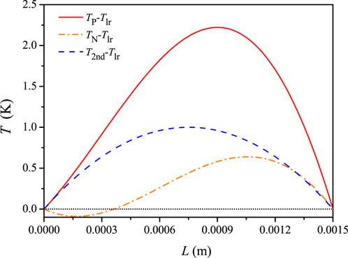
FIGURE 7. Comparisons on temperature distribution among the present, second-order, and linear models (T_h = 443 K and T_c = 323 K).

The developed numerical model can predict the response of temperature distribution under different external loads, which is shown in Figure 8. It is found that the ratio of the external load to internal electrical resistance (R_ex/R_in) considerably affects the temperature distribution. A conclusion can be obtained from Figure 8 by revising Eqs 1 and 12: the electric current notably affects the temperature distribution. A low R_ex/R_in results in a large current. Therefore, augmented Peltier heat pumping occurs, which leads to different temperature distributions. Note that the Thomson effect is also involved, and it is difficult to distinguish the influence level by the Thomson effect in Figure 8. However, more detailed results and discussions are presented in the following section related to this concern.

FIGURE 8

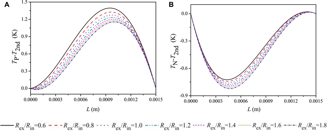
FIGURE 8. Influence of external load on temperature distribution along the TE leg. (A) P-type leg. (B) N-type leg (T_h = 443 K and T_c = 323 K).

3.4 Influence of the Thomson effect

An interesting exploration is to intentionally remove the Thomson term from Eq. 8, and the results are shown in Figure 9 and Figure 10. As shown in Figure 9, the temperature difference caused by the Thomson effect for the P-/N-type legs are considerable, and R_ex/R_in also plays an important role in causing the abovementioned temperature difference. By comparing Figures 6, 7, and 9, it is found that the influence of the local change rate of thermal conductivity and the Thomson effect in the P-type leg are in the same phase, which enlarges the temperature difference in Figure 7. However, the influence of the local change rate of thermal conductivity is out of phase with the influence of the Thomson effect in the N-type leg. Hence, the temperature difference of the N-type leg is smaller than that of the P-type leg as seen in Figure 7.

FIGURE 9

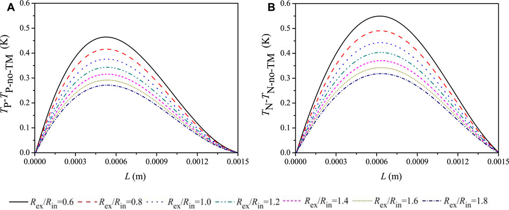
FIGURE 9. Influence of the Thomson effect on temperature distribution along the TE leg. (A) P-type leg. (B) N-type leg (T_h = 443 K and T_c = 323 K).

FIGURE 10

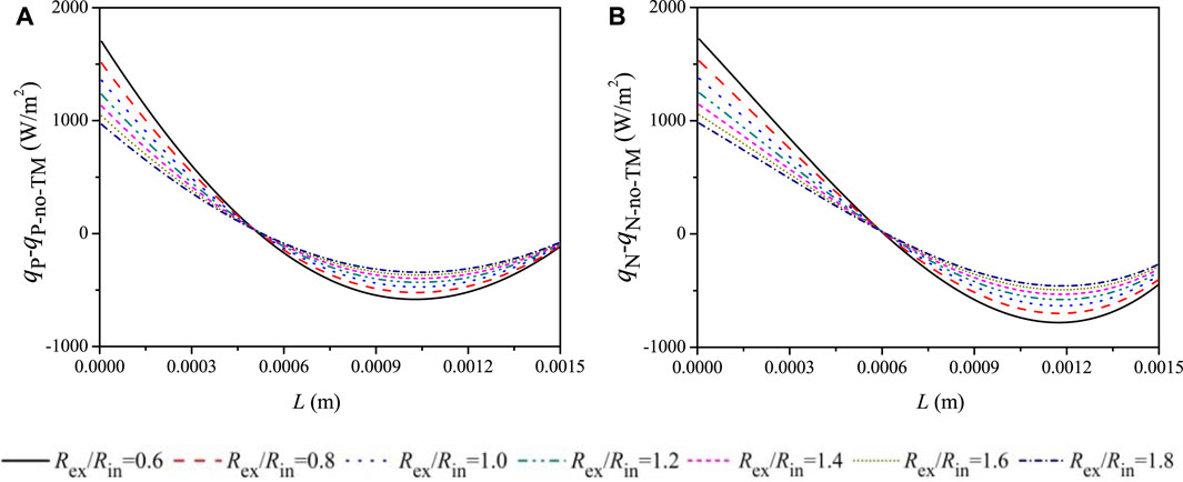
FIGURE 10. Influence of the Thomson effect on the heat flux along the TE leg. (A) P-type leg. (B) N-type leg (T_h = 443 K and T_c = 323 K).

The heat absorption and release by the Thomson effect are quantitatively shown in Figure 10. It is clearly seen that both heat absorption and release occur in the P-/N-type legs. That is, heat is released in a certain length of the leg near the cold-end of the TEM, whereas heat is absorbed in the remaining length of the leg near the hot-end of the TEM. The abovementioned phenomenon reveals the complicated nature of TE conversion.

3.5 Power generation and TE efficiency

The electric power (P) and TE efficiency (ξ) under different hot-end temperatures and R_ex/R_in are shown in Figure 11. Several sets of data are extracted from Figure 11A to compare with the experimental data as shown in Figure 4. For a constant cold-end temperature (323 K), the electric power is mainly determined by the hot-end temperature, and R_ex/R_in is another important parameter. A new finding shown in Figure 11A is that the obtained curve surface bends with a larger amplitude as the hot-end temperature increases. On the other hand, the TE efficiency monotonously increases with the temperature difference when constant material properties are assumed. However, the abovementioned monotonous increase is no longer existent when temperature-dependent material properties are considered. As shown in Figure 11B, the maximum TE efficiency is found to be near the hot-end temperature of 500 K and further increasing the hot-end temperature leads to lower TE efficiency than that near 500 K even though the electric power continues to increase, as shown in Figure 11A. The abovementioned phenomenon is caused by the fact that the thermal conductivity of the TE material monotonously increases with temperature, but the Seebeck coefficient exhibits a parabolic shape with temperature. Note that the TE efficiency could be over predicted because thermal resistances caused by substrates and copper pads, thermal/electrical contacts, and convective/radiative thermal leaks inside the TEM are not considered, which is stated in Section 2.1. However, this will not alter the conclusion of the present work.

FIGURE 11

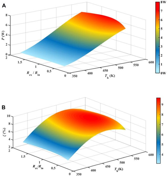
FIGURE 11. Power generation optimization under various external loads and temperature differences when T_c = 323 K. (A) Electric power. (B) TE efficiency.

3.6 Optimization of configuration

Figure 12 shows the structural optimization results concerning electric power and TE efficiency. The electric power can be customized according to particular applications because the electric power is sensitive to all structural parameters (a, L, and F). Note that the results in Figure 12 are obtained under the assumption that the thermal leaks by air conduction and thermal radiation inside the TEM are neglected. Minor influence on electric power is expected because the ratio of the thermal leak to the total heat flux passing through the TEM is only several percentages even though changing F results in different quantities of thermal leaks. Hence, Figure 12 presents valuable optimization results in the aspect of structure configuration. The ordinary method of predicting the electric power is to assume the temperature-dependent material properties as constants, i.e., averaged material properties between hot-/cold-ends. This assumption is effective, and only minor differences can be found when using the present numerical model, which is shown in Figure 12B. It is found that the electric power differences (P_max − P_maxav) are within 1% of the developed numerical model and the ordinary model with averaged material properties. P_maxav is the maximum electric power with average TE material properties.

FIGURE 12

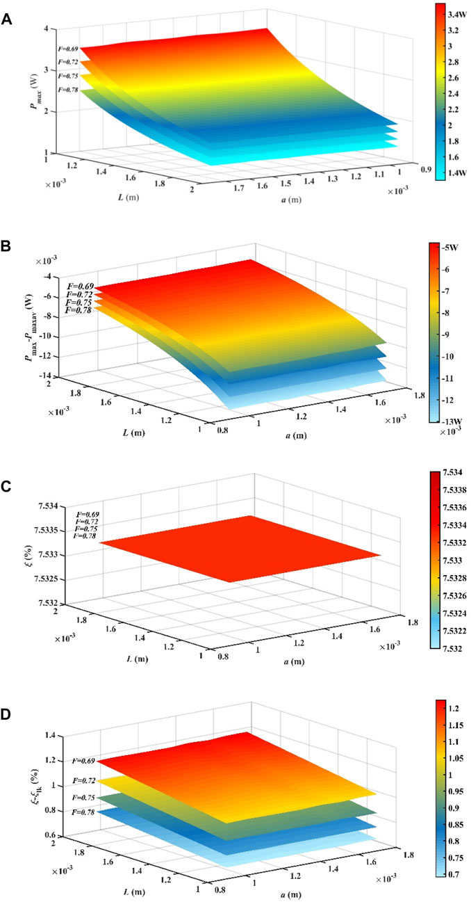
FIGURE 12. Influence of occupancy ratio, leg width, and leg length on power generation. (A) Maximum electric power (P_max). (B) Electric power difference (P_max − P_maxav) between temperature-dependent material properties and constant material properties. (C) TE efficiency (ξ) (four contour surfaces overlap with each other). (D) Difference in TE efficiency (ξ − ξ_lk) when considering thermal leaks inside the TEM.

TE efficiency remains unchanged under different structural parameters, as shown in Figure 12C. This reveals that an attempt to augment the TE efficiency with the same TE material through structural optimization has little potential. Note that the TE efficiency was found to be changed slightly when modifying the TEM structure (Zhao et al., 2021). This phenomenon is caused by the thermal leak inside the TEM (Lee et al., 2018). In case that Eq. 14 includes the conduction heat loss and radiative thermal loss between the hot-/cold-ends (Lee et al., 2018), the TE efficiency difference (ξ − ξ_lk) versus structural parameters is shown in Figure 12D, where ξ_lk is the TE efficiency when thermal leaks inside the TEM are considered in Eqs 13 and 14. As shown in Figure 12D, the major parameter affecting the TE efficiency is the occupancy ratio, and the leg length also plays a moderate influence on TE efficiency. The influence level by thermal leaks could reach up to 15%. A low occupancy ratio leads to a serious downgrade of TE efficiency. The influence of thermal leaks on the TE efficiency is not the major task of the present work.

4 Conclusion

A one-dimensional numerical model was developed to include Seebeck, Joule, Peltier, and Thomson effects. No simplifications are required for the temperature-dependent material properties. The numerical model was verified with experiments and the following conclusions were drawn on the basis of comprehensively analyzing the temperature distribution, heat flux, Thomson influence, electric power, and TE efficiency:

(1) The local change rate of thermal conductivity considerably affects the temperature distributions along the TE leg. The second-order central finite difference algorithm is suggested to consider the local change rate of thermal conductivity.

(2) Temperature distributions considering temperature-dependent material properties are in-consistent with the parabolic temperature distributions. Much larger temperature divergence is found when compared with the parabolic temperature distribution. The location of maximum temperature divergence shifts from the leg’s central location to other positions.

(3) The Thomson effect considerably affects the temperature distribution, and the influence level can be as large as 0.5 K. Moreover, heat is released in a certain length of the leg near the cold-end of the TEM due to the Thomson effect, whereas heat is absorbed in a certain length of the leg near the hot-end of the TEM.

(4) The parabolic-like distribution of TE efficiency versus running temperature can be captured by the developed numerical model, which is caused by the temperature-dependent material properties.

(5) The ordinary method to predict the electric power using averaged material properties between hot-/cold-ends are effective. The developed numerical model confirms the abovementioned ordinary method, and only minor difference is found when temperature-dependent material properties are fully considered.

(6) The attempt to perform structural optimization aiming to significantly augment the TE efficiency with the same TE material has little potential. The possible enhancement of TE efficiency through structural optimization is contributed by minimizing thermal leaks inside the TEM.

Data availability statement

The original contributions presented in the study are included in the article/Supplementary Material; further inquiries can be directed to the corresponding author.

Author contributions

CX: Investigation and manuscript writing—original draft. SH: Data curation, validation, and manuscript writing—original draft. HL: Data curation, investigation, and manuscript writing—review and editing. GL: Conceptualization, funding acquisition, methodology, and manuscript writing—review and editing. YF: Formal analysis, investigation, and manuscript writing—original draft. SW: Methodology, project administration, and manuscript writing—original draft. CXu: Resources, visualization, and manuscript writing—original draft. WG: Investigation, validation, and manuscript writing—review and editing.

Funding

The author(s) declare that financial support was received for the research, authorship, and publication of this article. This work was supported by the Science and Technology Project of State Grid Zhejiang Electric Power Co., Ltd. (Grant No. 5211UZ230002), the Key Program of Natural Science Foundation of Zhejiang Province (Grant no. LZ21E060001), and the Key R&D Plan of Zhejiang Province (Grant no. 2020C03115).

Conflict of interest

Authors CX, SH, YF, SW, and CXu were employed by the State Grid Huzhou Power Supply Company. Author HL is employed by TBEA Hengyang Transformer Co., Ltd.

The remaining authors declare that the research was conducted in the absence of any commercial or financial relationships that could be construed as a potential conflict of interest.

Publisher’s note

All claims expressed in this article are solely those of the authors and do not necessarily represent those of their affiliated organizations, or those of the publisher, editors, and reviewers. Any product that may be evaluated in this article, or claim that may be made by its manufacturer, is not guaranteed or endorsed by the publisher.

References

Alghoul, M. A., Shahahmadi, S. A., Yeganeh, B., Asim, N., Elbreki, A. M., Sopian, K., et al. (2018). A review of thermoelectric power generation systems: roles of existing test rigs/prototypes and their associated cooling units on output performance. Energ. Convers. manage. 174, 138–156. doi:10.1016/j.enconman.2018.08.019

CrossRef Full Text | Google Scholar

Cui, Y. J., Wang, K. F., Wang, B. L., Li, J. E., and Zhou, J. Y. (2019). A comprehensive analysis of delamination and thermoelectric performance of thermoelectric pn-junctions with temperature-dependent material properties. Compos. Struct. 229, 111484. doi:10.1016/j.compstruct.2019.111484

CrossRef Full Text | Google Scholar

Eldesoukey, A., and Hassan, H. (2019). 3D model of thermoelectric generator (TEG) case study: effect of flow regime on the TEG performance. Energ. Convers. manage. 180, 231–239. doi:10.1016/j.enconman.2018.10.104

CrossRef Full Text | Google Scholar

Fraisse, G., Ramousse, J., Sgorlon, D., and Goupil, C. (2013). Comparison of different modeling approaches for thermoelectric elements. Energ. Convers. manage. 65, 351–356. doi:10.1016/j.enconman.2012.08.022

CrossRef Full Text | Google Scholar

Hinterleitner, B., Knapp, I., Poneder, M., Shi, Y., Müller, H., Eguchi, G., et al. (2019). Thermoelectric performance of a metastable thin-film Heusler alloy. Nature 576, 85–90. doi:10.1038/s41586-019-1751-9

PubMed Abstract | CrossRef Full Text | Google Scholar

Ju, C., Dui, G., Zheng, H. H., and Xin, L. (2017). Revisiting the temperature dependence in material properties and performance of thermoelectric materials. Energy 124, 249–257. doi:10.1016/j.energy.2017.02.020

CrossRef Full Text | Google Scholar

Lee, H., Sharp, J., Stokes, D., Pearson, M., and Priya, S. (2018). Modeling and analysis of the effect of thermal losses on thermoelectric generator performance using effective properties. Appl. Energ. 211, 211 987–996. doi:10.1016/j.apenergy.2017.11.096

CrossRef Full Text | Google Scholar

Li, G., Yi, M., Tulu, M. B., Zheng, Y., Guo, W., and Tang, Y. (2021). Miniature self-powering and self-aspirating combustion-powered thermoelectric generator burning gas fuels for combined heat and power supply. J. Power Sources 506, 230263. doi:10.1016/j.jpowsour.2021.230263

CrossRef Full Text | Google Scholar

Li, G., Zheng, Y., Guo, W., Zhu, D., and Tang, Y. (2020a). Mesoscale combustor-powered thermoelectric generator: experimental optimization and evaluation metrics. Appl. Energ. 272, 115234. doi:10.1016/j.apenergy.2020.115234

CrossRef Full Text | Google Scholar

Li, G., Zheng, Y., Hu, J., and Guo, W. (2019). Experiments and a simplified theoretical model for a water-cooled, stove-powered thermoelectric generator. Energy 185, 437–448. doi:10.1016/j.energy.2019.07.023

CrossRef Full Text | Google Scholar

Li, G., Zhu, D., Zheng, Y., and Guo, W. (2020b). Mesoscale combustor-powered thermoelectric generator with enhanced heat collection. Energ. Convers. manage. 205, 112403. doi:10.1016/j.enconman.2019.112403

CrossRef Full Text | Google Scholar

Lin, Q., Chen, Y., Chen, F., DeGanyar, T., and Yin, H. (2022). Design and experiments of a thermoelectric-powered wireless sensor network platform for smart building envelope. Appl. Energ. 305, 117791. doi:10.1016/j.apenergy.2021.117791

CrossRef Full Text | Google Scholar

Liu, K., Tang, X., Liu, Y., Xu, Z., Yuan, Z., Ji, D., et al. (2020). Experimental optimization of small–scale structure–adjustable radioisotope thermoelectric generators. Appl. Energ. 280, 115907. doi:10.1016/j.apenergy.2020.115907

CrossRef Full Text | Google Scholar

Luo, D., Yan, Y., Li, Y., Wang, R., Chen, S., Yang, X., et al. (2023). A hybrid transient CFD-thermoelectric numerical model for automobile thermoelectric generator systems. Appl. Energ. 332, 120502. doi:10.1016/j.apenergy.2022.120502

CrossRef Full Text | Google Scholar

Lv, S., He, W., Hu, Z., Liu, M., Qin, M., Shen, S., et al. (2019). High-performance terrestrial solar thermoelectric generators without optical concentration for residential and commercial rooftops. Energ. Convers. manage. 196, 69–76. doi:10.1016/j.enconman.2019.05.089

CrossRef Full Text | Google Scholar

Manikandan, S., and Kaushik, S. C. (2016). The influence of Thomson effect in the performance optimization of a two stage thermoelectric generator. Energy 100, 227–237. doi:10.1016/j.energy.2016.01.092

CrossRef Full Text | Google Scholar

Min, G. (2022). New formulation of the theory of thermoelectric generators operating under constant heat flux. Energy Environ. Sci. 15, 356–367. doi:10.1039/d1ee03114g

CrossRef Full Text | Google Scholar

Nozariasbmarz, A., Collins, H., Dsouza, K., Polash, M. H., Hosseini, M., Hyland, M., et al. (2020). Review of wearable thermoelectric energy harvesting: from body temperature to electronic systems. Appl. Energ. 258, 114069. doi:10.1016/j.apenergy.2019.114069

CrossRef Full Text | Google Scholar

Ponnusamy, P., de Boor, J., and Müller, E. (2020). Discrepancy between constant properties model and temperature-dependent material properties for performance estimation of thermoelectric generators. Entropy 22, 1128. doi:10.3390/e22101128

PubMed Abstract | CrossRef Full Text | Google Scholar

Pourkiaei, S. M., Ahmadi, M. H., Sadeghzadeh, M., Moosavi, S., Pourfayaz, F., Chen, L., et al. (2019). Thermoelectric cooler and thermoelectric generator devices: a review of present and potential applications, modeling and materials. Energy 186, 115849. doi:10.1016/j.energy.2019.07.179

CrossRef Full Text | Google Scholar

Rowe, D. M. (1995). CRC handbook of thermoelectrics. Location, London: CRC Press.

Google Scholar

Rowe, D. M., and Gao, M. (1998). Evaluation of thermoelectric modules for power generation. J. Power Sources 73, 193–198. doi:10.1016/s0378-7753(97)02801-2

CrossRef Full Text | Google Scholar

Shen, L., Wang, Y., Tong, X., Xu, S., and Sun, Y. (2021). Inverse optimization investigation for thermoelectric material from device level. Energ. Convers. manage. 228, 113669. doi:10.1016/j.enconman.2020.113669

CrossRef Full Text | Google Scholar

Shen, Z., Tian, L., and Liu, X. (2019). Automotive exhaust thermoelectric generators: current status, challenges and future prospects. Energ. Convers. manage. 195, 1138–1173. doi:10.1016/j.enconman.2019.05.087

CrossRef Full Text | Google Scholar

Sun, Y., Chen, G., Duan, B., Li, G., and Zhai, P. (2019). An annular thermoelectric couple analytical model by considering temperature-dependent material properties and Thomson effect. Energy 187, 115922. doi:10.1016/j.energy.2019.115922

CrossRef Full Text | Google Scholar

Sun, Z., Luo, D., Wang, R., Li, Y., Yan, Y., Cheng, Z., et al. (2022). Evaluation of energy recovery potential of solar thermoelectric generators using a three-dimensional transient numerical model. Energy 256, 124667. doi:10.1016/j.energy.2022.124667

CrossRef Full Text | Google Scholar

Wee, D. (2011). Analysis of thermoelectric energy conversion efficiency with linear and nonlinear temperature dependence in material properties. Energ. Convers. manage. 52, 3383–3390. doi:10.1016/j.enconman.2011.07.004

CrossRef Full Text | Google Scholar

Wee, D. (2018). Uncertainty and sensitivity of the maximum power in thermoelectric generation with temperature-dependent material properties: an analytic polynomial chaos approach. Energ. Convers. manage. 157, 103–110. doi:10.1016/j.enconman.2017.11.088

CrossRef Full Text | Google Scholar

Zhao, Z., Zuo, Z., Wang, W., Liu, R., and Kuang, N. (2021). Performance optimization for a combustion-based micro thermoelectric generator with two-stage thermoelectric module. App. Therm. Eng. 198, 117464. doi:10.1016/j.applthermaleng.2021.117464

CrossRef Full Text | Google Scholar