Meta-reservoir computing for learning a time series predictive model of wind power

1 Introduction

The utilization of wind power has dramatically improved in the last decade. Wind power generation is random due to the uncertain property of wind speed. The uncertainty of wind power generation brings challenges to the power system dispatch with safety constraints and operational stability (Ummels et al., 2007). Thus, accurate wind turbine power generation prediction is critical for improving the safety and efficiency of utilizing wind energy in power systems (Lange, 2005). Nowadays, wind turbines are often equipped with Supervisory Control and Data Acquisition (SCADA) systems that record the real-time data on wind turbine operations. The data from the SCADA system can be applied to monitor the status of the wind turbines. On the other hand, we can also use the data to build predictive models for wind turbine power.

The research on wind power prediction has been mainly focused on providing time series predictions based on time series data (Burke and O’Malley, 2011). Deep learning models have been applied to improve the accuracy of wind power prediction. One mainstream method is to use a long short-term memory (LSTM) neural network to model the time series wind power model. For example, Chen et al. (2019) proposed a two-layer method, which combines extreme learning machine and LSTM to address the nonlinear property of the wind power model and overcome the weakness of linear combination by using only one layer. In addition, Ko et al. (2021) proposed a deep residual network that integrates long and short bidirectional LSTM to improve accuracy and training efficiency further. Recently, a probabilistic prediction of wind power has also been addressed. Zhang et al. (2021) designed a multi-source and temporal attention network to improve prediction performance by introducing three specific designed sources. Furthermore, Safari et al. (2018) used ensemble empirical mode decomposition to divide the wind power time series into different components with different time–frequency characteristics. Then, the authors used chaotic time series analysis to discover the components with chaotic properties. Subsequently, the predictive model provides the predictions for the chaotic and nonchaotic parts separately, which improves the prediction accuracy. Zhao et al. (2021) proposed an integrated probabilistic forecasting and decision framework to optimize the prediction interval of wind power and quantify the probabilistic reserve simultaneously. An extreme learning machine is applied to reduce the time efficiency of establishing the prediction interval. In addition, a novel closed-form prediction for wind speed and wind power is presented by Wang et al. (2021). Liu et al. (2018)integrated wavelet packet decomposition, gray wolf optimizer, adaptive boosting.MRT, and robust extreme learning machine to increase the accuracy of multi-step prediction for wind power.

Recent research has discovered that the wind speed dynamical model and the wind turbine power curve depend on the environment, such as atmospheric conditions and temperature (Cascianelli et al., 2022; Pandit et al., 2023). None of the above research on wind power predictive models has considered environmental changes. Wu et al. (2023) presented a heuristic result that considers the atmospheric model in wind power prediction. However, it does not give hints on building a more general model. Deep models encounter overfitting issues (Duffy et al., 2023). As the environment changes, the prediction by deep models deviates from the real value and needs to be modified by using data from the new environment. The traditional training methods for deep models need a sufficiently large number to train the model, which is computationally complex for real-time modification. In addition, it may not be practical to quickly obtain many new data.

The reservoir computing method is a computationally efficient method to train neural network models (Hamedani et al., 2018; Nokkala et al., 2022), including recurrent neural networks (RNNs) and LSTM neural networks. Although using the reservoir computing method for deep models can significantly reduce the computational complexity for training, the issue of not having enough data quickly is still unresolved. Meta-learning has been validated to adapt the deep model to a new situation with only a few shots of data (Li and Hu, 2021; Tian et al., 2022). This paper combines the advantages of reservoir computing and meta-learning and proposes a novel wind power predictive model, named the meta-reservoir computing method. Meta-learning optimizes part of the hyperparameters of the reservoir computing algorithm based on a multiple-task dataset. Then, the enhanced reservoir computing algorithm can efficiently adapt the predictive model of wind power to a new task with a few data samples. We conducted experimental data-based validations to evaluate the proposed meta-reservoir computing method. The main contributions of this paper are summarized as follows:

• This is the first study to consider the problem of adapting a deep learning wind power predictive model with small samples.

• Meta-learning is combined with reservoir computing for the first time to improve the training efficiency of deep learning models for wind power prediction with the constraint of small samples.

The remainder of this paper is organized as follows: Section 2 presents the addressed problem after formulating the model, integrating the environment factors; Section 3 explains the proposed meta-reservoir computing method for wind power predictive modeling; Section 4 presents the validation results of applying the proposed meta-reservoir computing method to an experimental dataset; and Section 5 presents the conclusions of this paper.

2 Addressed problem: fast model learning for wind power prediction

Let the time index be k = 0, 1, 2, … , T, …. At every time k, the wind power is defined by p_k. Wind power is generated from the wind turbine and depends on the wind speed at the current time index k. Let s_k be the wind speed at time step k. A nonlinear map called the wind turbine power curve (Luo et al., 2022) describes the correlation between wind speed and wind power output, which is expressed as follows:

$p_k=h\left(s_k,w_k\right),(1)$

where w_k defines the uncertainty related to the measurements and the model bias.

On the other hand, the mechanism of generating wind speed s_k is essentially a Markov process defined by

$s_{k+1}=f\left(s_k,v_k\right),(2)$

where v_k is the system noise and f(⋅) is the function that describes the state transition with randomness. Note that the randomness is addressed by the system noise v_k. Then, we can equivalently regard the wind power itself following a Markov process defined by

$p_{k+1}=g\left(p_k,{\delta }_k\right).(3)$

In practice, g(⋅) is not available. One basic solution is to use the time series dataset of wind power to estimate g(⋅), which essentially follows a data-driven fashion. Let

${\mathcal{D}}_T≔{\left\{p_k\right\}}_{k=0}^T(4)$

be the available dataset. The traditional problem is to solve

$\underset{\tilde{g}}{\min }\sum _{k=0}^{T-1}{\left(p_{k+1}-\tilde{g}\left(p_k\right)\right)}^2.(5)$

However, recent research reveals that the wind speed dynamical model and the wind turbine power curve vary as the environment changes (Cascianelli et al., 2022; Pandit et al., 2023). Namely, instead of using (Eqs 1, 2), the following model should be used:

$p_k=h\left(s_k,\theta ,w_k\right),(6)$

$s_{k+1}=f\left(s_k,\theta ,v_k\right),(7)$

where θ defines an unknown variable to represent the influence of the environment change. Then, the dynamical model of the wind power is written by

$p_{k+1}=g\left(p_k,\theta ,{\delta }_k\right).(8)$

Suppose the dataset ${\mathcal{D}}_T$ includes the data collected from different environments specified by labels from {1, … , K}. If we train the model $\tilde{g}$ by solving Eq. 5 directly based on ${\mathcal{D}}_T$, the solution will not fit any model conditioned on the label i, i = 1, … , K. On the other hand, when the new dataset ${\mathcal{D}}_{T^{\prime }}^{K+1}$ conditioned on a new environment specified by θ_K+1 comes with very few samples (namely, T′ is very small), there is no effective way to adapt the solution to dataset ${\mathcal{D}}_T$ to the new environment model.

This paper addresses the problem of providing a solution ${\tilde{g}}^{*}$ robust to each environment parameter θ_i, i = 1, … , K. On the other hand, ${\tilde{g}}^{*}$ should also have a property that it can be adapted to the solution of a new set, ${\tilde{g}}_{K+1}$, very efficiently, with only very few data obtained on the new environment.

3 Meta-reservoir computing for wind power prediction

3.1 Reservoir computing

Reservoir computing is a computational approach for time series data processing based on neural networks. Reservoir computing was first proposed by Jaeger and Haas (2004) for optimizing RNN models for given training data. Since RNN is widely used for time series data modeling, reservoir computing can also be generalized to the applications of time series data processing (Tanaka et al., 2019).

In reservoir computing, the time series data are supposed to be generated from unknown dynamical models driven by sequences of inputs, and the system outputs sequences of outputs. It can also be applied to autonomous systems by setting the input at each time as zero. In this paper, since we do not have input for the dynamics of wind speed, the input is not considered. The reservoir in reservoir computing is essentially the state variable of the established dynamical model for predicting the output, and it does not have to represent the underlying state of the actual physical systems (Tanaka et al., 2019). Let r_k be the reservoir at time step k. The measured output at time step k is defined by y_k. The reservoir at time step k + 1, r_k+1, is a function of r_k and y_k, written by

${\mathbf{r}}_{k+1}={\mathbf{f}}_{\text{rc}}\left({\mathbf{W}}_{\text{rc}}{\mathbf{r}}_k+{\mathbf{W}}_{\text{back}}{\mathbf{y}}_{\mathit{k}}\right),(9)$

where f_rc is a neural network and W_rc and W_back are the weight matrices for reservoir–reservoir connections and output–reservoir connections, respectively. The output at time index k + 1 is predicted by

${\mathbf{y}}_{k+1}={\mathbf{W}}_{\text{out}}{\mathbf{r}}_{k+1}.(10)$

The computational complexity is immense if we want to train W_out, W_back, and W_rc together. Note that the model capacity is substantial if there are enough reservoirs and neurons. The model can achieve high accuracy even though W_back and W_rc are randomly given and only W_out is trained. The algorithm of implementing reservoir computing with a dataset ${\mathcal{D}}_T^{\text{rc}}≔{\left\{{\mathbf{y}}_k\right\}}_{k=0}^T$ is summarized in Algorithm 1.

Algorithm 1.Implementation of reservoir computing for a time series dataset ${\mathcal{D}}_{\mathcal{T}}^{\mathbf{r}\mathbf{c}}$.

Inputs: dataset ${\mathcal{D}}_T^{\text{rc}}={\{{\mathbf{y}}_k\}}_{k=0,\dots ,T}$

  1: Select the model f_rc and reservoir r_k

  2: Generate weight matrices W_back and W_rc randomly

  3: Generate initial reservoir r₀ randomly

  4: Obtain the weight matrix W_out by solving the following problem

$\min \sum _{k=0}^T{‖{\mathbf{W}}_{\text{out}}{\mathbf{r}}_k-{\mathbf{y}}_k‖}^2+\lambda \Vert {\mathbf{W}}_{\text{out}}{\Vert }_2^2(11)$

Output: Initial reservoir r₀, Weight matrices W_out, W_back, and W_rc

Note that λ is a parameter for regularization. Using a large λ confers the method a higher robustness but may lose some accuracy. With a small λ, the obtained model will have better accuracy but may encounter the overfitting issue. The choice of λ should be made according to the problem and the user demands.

3.2 Meta-learning

The meta-learning discussion first focused on learning in a multiple-task scenario. To specify the training process of meta-learning, it is formulated as a bi-level optimization problem. We will clearly explain how the bi-level optimization framework of meta-learning fits our problem.

As introduced in Section 2, the dataset ${\mathcal{D}}_T$ includes the data obtained from different environments specified by the task labels {1, … , K}. Then, the dataset can be divided into K different tasks. Each task has a corresponding dataset ${\mathcal{D}}_{T_i}^i,i=1,\dots ,K$. Instead of only considering the parameter vector in the model to be learned in meta-learning, another important variable, ω, which specifies the algorithm about how to learn the parameter, is also optimized. The variable ω can include the initial point of the parameter, the hyperparameters for the gradient-descent method, the choice of cost function, and the selected model.

The dataset of each task is separated into a training set ${\mathcal{D}}_{T_i}^{i,\mathrm{t}\mathrm{r}}$ and test set ${\mathcal{D}}_{T_i}^{i,\mathrm{t}\mathrm{e}}$. Note that the parameter obtained by each dataset depends not only on the training dataset but also on the learning variable ω. The loss function depends on the trained parameter vector. Let ${\mathcal{L}}^{\text{train}}(\cdot )$ and ${\mathcal{L}}^{\text{test}}(\cdot )$ be the loss function for training and testing, respectively. Then, the training process in meta-learning can be formulated as

$\underset{\omega }{\min }\sum _{i=1}^K{\mathcal{L}}^{\text{test}}\left({\mathcal{D}}_{T_i}^{i,\mathrm{t}\mathrm{e}},{\theta }_{*}^{\left(i\right)}\left(\omega \right),\omega \right),(12)$

$\mathrm{s}.\mathrm{t}.{\theta }_{*}^{\left(i\right)}\left(\omega \right)=\arg \underset{\theta }{\min }{\mathcal{L}}^{\text{train}}\left({\mathcal{D}}_{T_i}^{i,\mathrm{t}\mathrm{r}},\theta ,\omega \right),i=1,\dots ,K.(13)$

Let ω* be the solution to the bi-level optimization problem. In every iteration, the learning parameter ω is optimized for a given θ, and finally, it converges to the optimal value for learning a task. The optimality here refers to the given training dataset. Even for a newly given task, the learning parameter ω* can provide better efficiency to find the optimal parameter for the newly given task.

3.3 Algorithm for meta-reservoir computing

This paper proposes a novel wind power predictive model learning algorithm that combines reservoir computing and meta-learning. As introduced in Section 2, we have the dataset ${\mathcal{D}}_T$ obtained from multiple environments. Regarding each environment as a task, we separate the dataset into

${\mathcal{D}}^i≔{\left\{p_k^{\left(i\right)}\right\}}_{k=0}^{T_i},i=1,\dots ,K.(14)$

Note that we have

$\bigcup _{i=1}^K{\mathcal{D}}^i={\mathcal{D}}_T(15)$

and

${\mathcal{D}}^i\bigcap {\mathcal{D}}^j=\varnothing ,\text{if}i\ne j.(16)$

For each task, we further separate the dataset into data for training and data for testing as follows:

${\mathcal{D}}_{\text{train}}^i≔{\left\{p_k^{\left(i\right),\mathrm{t}\mathrm{r}\mathrm{a}\mathrm{i}\mathrm{n}}\right\}}_{k=0}^{T_{i,\mathrm{t}\mathrm{r}\mathrm{a}\mathrm{i}\mathrm{n}}},{\mathcal{D}}_{\text{test}}^i≔{\left\{p_k^{\left(i\right),\mathrm{t}\mathrm{e}\mathrm{s}\mathrm{t}}\right\}}_{k=0}^{T_{i,\mathrm{t}\mathrm{e}\mathrm{s}\mathrm{t}}}.(17)$

Note that we have

${\mathcal{D}}_{\text{train}}^i\bigcap \underset{\text{test}}{\overset{i}{\mathcal{D}}}=\varnothing ,(18)$

${\mathcal{D}}_{\text{train}}^i\bigcup \underset{\text{test}}{\overset{i}{\mathcal{D}}}={\mathcal{D}}^i,(19)$

for every task i = 1, … , K.

We use reservoir computing to train a temporal prediction model of wind power. Thus, the parameter to be trained is ${\mathbf{W}}_{\text{out}}^{(i)}$. There are a lot of hyperparameters to be optimized, such as the initial point of reservoirs, the initial point of the solution of the optimization problem for obtaining ${\mathbf{W}}_{\text{out}}^{(i)}$, the gradient-descent rate, and the ratio λ for regularization. This study adopts the initial point of the solution to the optimization problem, W_out(0), and the initial point of reservoirs r₀ as the learning parameter ω*. Namely, we have

${\omega }^{*}=\left({\mathbf{W}}_{\text{out}}\left(0\right),{\mathbf{r}}_0\right).(20)$

Note that the learning parameter ω* is common for each task, and the parameter differs in each task. For the loss function, we adopt the loss function of Eq. 11 for both training and testing processes. It is written as

$\begin{array}{ll}\hfill & {\mathcal{L}}^{\text{train}}\left({\mathcal{D}}_{\text{train}}^i,{\mathbf{W}}_{\text{out}}^{\left(i\right)},\omega \right)\hfill \\ \hfill & =\sum _{k=0}^{T_{i,\mathrm{t}\mathrm{e}\mathrm{s}\mathrm{t}}}{‖W_{\text{out}}^{\left(i\right)}{\mathbf{r}}_k^{\left(i\right)}-p_k^{\left(i\right),\mathrm{t}\mathrm{r}\mathrm{a}\mathrm{i}\mathrm{n}}‖}^2+\lambda \Vert {\mathbf{W}}_{\text{out}}^{\left(i\right)}{\Vert }_2^2,\hfill \end{array}(21)$

$\begin{array}{ll}\hfill & {\mathcal{L}}^{\text{test}}\left({\mathcal{D}}_{\text{train}}^i,{\mathbf{W}}_{\text{out}}^{\left(i\right),*},\omega \right)\hfill \\ \hfill & =\sum _{k=0}^{T_{i,\mathrm{t}\mathrm{r}\mathrm{a}\mathrm{i}\mathrm{n}}}{‖W_{\text{out}}^{\left(i\right),*}{\mathbf{r}}_k^{\left(i\right)}-p_k^{\left(i\right),\mathrm{t}\mathrm{e}\mathrm{s}\mathrm{t}}‖}^2+\lambda \Vert {\mathbf{W}}_{\text{out}}^{\left(i\right),*}{\Vert }_2^2.\hfill \end{array}(22)$

Then, the training process in meta-reservoir computing is written as

$\underset{\omega }{\min }\sum _{i=1}^K{\mathcal{L}}^{\text{test}}\left({\mathcal{D}}_{\text{train}}^i,{\mathbf{W}}_{\text{out}}^{\left(i\right),*},\omega \right),(23)$

$\mathrm{s}.\mathrm{t}.{\mathbf{W}}_{\text{out}}^{\left(i\right),*}=\arg \underset{{\mathbf{W}}_{\text{out}}^{\left(i\right)}}{\min }{\mathcal{L}}^{\text{train}}\left({\mathcal{D}}_{\text{train}}^i,{\mathbf{W}}_{\text{out}}^{\left(i\right)},\omega \right),i=1,\dots ,K.(24)$

According to the above discussions, we summarize the meta-reservoir computing algorithm for learning a wind power predictive model in Algorithm 2.

Algorithm 2.Implementation of meta-reservoir computing for learning a wind power predictive model.

Inputs: dataset ${\mathcal{D}}_T={\{p_k\}}_{k=0,\dots ,T}=\left\{{\mathcal{D}}_{\text{train}}^1,{\mathcal{D}}_{\text{test}}^1,\dots \dots ,{\mathcal{D}}_{\text{train}}^K,{\mathcal{D}}_{\text{test}}^K\right\}$, the regularization ratio λ, a new dataset ${\mathcal{D}}_{T^{\prime }}^{K+1}$

  1: Select the model f_rc and reservoir r_k

  2: Generate weight matrices W_back and W_rc randomly

  3: Solve the problem described by Eqs 23, 24 with dataset ${\mathcal{D}}_T$ and obtain ω*

  4: Obtain the weight matrix ${\mathbf{W}}_{\text{out}}^{(K+1)}$ by solving the following problem described by Eq. 11 with dataset ${\mathcal{D}}_{T^{\prime }}^{K+1}$, parameters f_rc, r_k, ω*, W_back, and W_rc

Output: $\omega =\left({\mathbf{r}}_0,{\mathbf{W}}_{\text{out}}(0)\right)$, weight matrices ${\mathbf{W}}_{\text{out}}^{K+1}$, W_back, and W_rc

4 Experimental validation

In this section, we first introduce the experimental dataset and several settings for validation. The validation results are then presented with detailed discussions.

4.1 Dataset for validation

This validation uses the experimental dataset shown in Figure 1. This dataset includes time series data obtained from eight different environments, as shown in Figures 1A–H, respectively. In addition, for each environment, we have 13 different profiles. The same environment means that the data were collected in the same period, places, and weather.

FIGURE 1

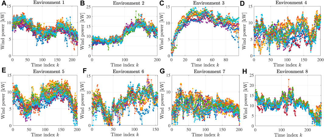
FIGURE 1. Experimental data used in this validation. The dataset includes data from eight different environments, plotted in (A–H). For each environment, there are 13 different profiles.

For meta-learning, seven profiles in each environment are used as training data and the rest as test data. For a fair comparison, we compare our MRC with normal reservoir computing (RC) without meta-learning. In each validation, we use data from seven environments to train a model and then use the rest for validation.

The comparison of the implementations of the MRC and RC methods is shown in Figure 2. For RC methods, the training set is used to train a recurrent neural network. We obtain only a parameter vector for the recurrent neural network. When a new task comes as a test set, only a few shots in the test set are used for training a new recurrent neural network. The trained parameter vector can be used as the initial value of reservoir computing for updating the recurrent neural network for the new task. For MRC methods, the training set is used for meta-learning. Except for one parameter vector for the training set, the learning parameter, including a good initial point, is also obtained. When a new task comes, the learning parameter is used to learn a new parameter vector for the new task.

FIGURE 2

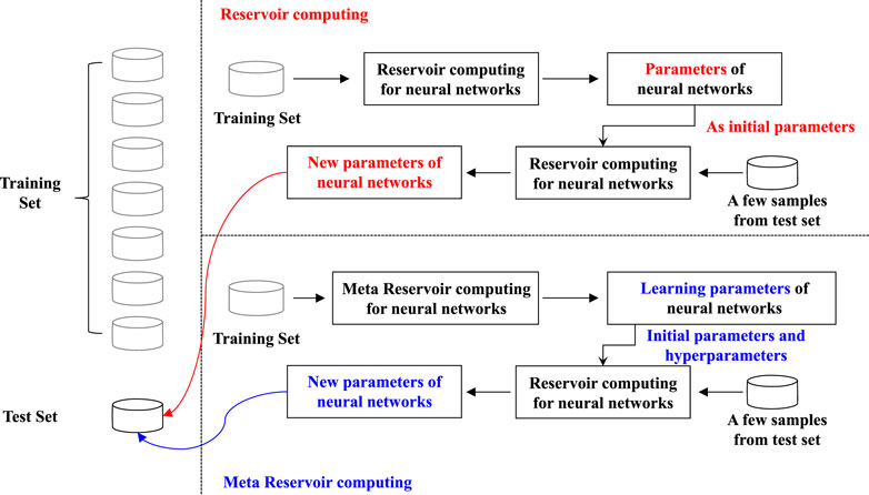
FIGURE 2. Implementations of the meta-reservoir computing and reservoir computing methods.

4.2 Validation results

The performance of the MRC and RC methods is evaluated by checking the accuracy of the model learned by each method with a fine-tuning process based on a sample number of 15 or 30 from a new task. During fine-tuning, each gradient-descent step is computed with the same data points. Figures 3, 4 provide the qualitative results for using environments 5 and 6 for the test. The red solid line is the model trained by using all the data in the test set, which can be regarded as a perfect model. The results show that the MRC method can provide a model very close to perfection, even with a few shots of data. Note that both MRC and RC methods do not have good initial points. However, the MRC method can adapt the model very quickly. The RC method fails to adapt the model to a proper model with the limited data number.

FIGURE 3

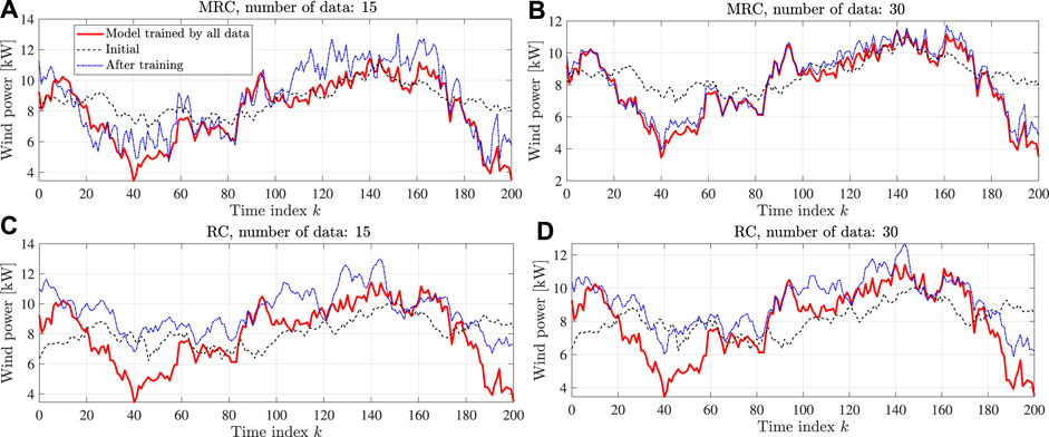
FIGURE 3. Few-shot adaptation for environment 5. (A) MRC with 15 samples; (B) MRC with 30 samples; (C) RC with 15 samples; and (D) RC with 30 samples.

FIGURE 4

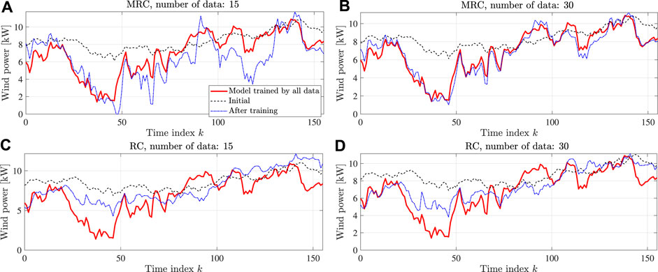
FIGURE 4. Few-shot adaptation for environment 6. (A) MRC with 15 samples; (B) MRC with 30 samples; (C) RC with 15 samples; and (D) RC with 30 samples.

Figure 5 provides more quantitative prediction results. The mean square errors (MSEs) of the model at each iteration are plotted for each case with a different environment as the test set. It is obvious that the proposed MRC method can adapt the model to a given environment even though the initial MSE is almost the same as that of the RC method. The reason is that the MRC method optimizes the initial value of the reservoir, which may provide some information to find a better gradient to reduce the loss. The intuitive explanation is given in Figure 6.

FIGURE 5

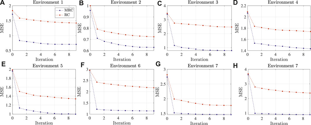
FIGURE 5. Quantitative prediction results showing the MSE curve along with the training iteration (30 samples): (A) Environment 1; (B) Environment 2; (C) Environment 3; (D) Environment 4; (E) Environment 5; (F) Environment 6; (G) Environment 7; (G) Environment 8.

FIGURE 6

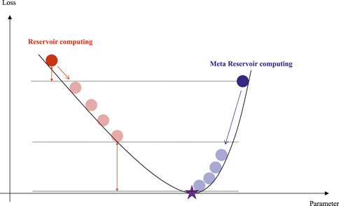
FIGURE 6. Intuitive explanation of the quantitative prediction results.

5 Conclusion

A wind power prediction model must be able to be adapted to a new environment, with a few samples of data from the new environment. The traditional deep learning methods encounter the overfitting issue and are hard to be adapted to a new environment. A huge dataset is still needed. This paper proposes a novel learning method for a wind power prediction model. The reservoir computing algorithm is combined with meta-learning to efficiently adapt the wind power prediction model to a new environment with only a few samples. The algorithmic structure of reservoir computing significantly reduces the computational complexity of learning a deep model. On the other hand, the initial points and other hyperparameters of reservoir computing are optimized by meta-learning based on the historical dataset. Experimental datasets have validated the proposed meta-reservoir computing method for learning the wind power prediction model. The validation results show that the proposed meta-reservoir computing can find a good model for the new environment in a very small number of iterations with a few shots of new data.

The proposed method opens a new avenue for training wind power predictive models for different environments. Instead of giving the best point for each environment, it is better to find a good learning parameter to be ready for new tasks. In future work, we will investigate comparing the proposed method with more existing deep models.

Data availability statement

The original contributions presented in the study are included in the article/Supplementary Material, further inquiries can be directed to the corresponding author.

Author contributions

LZ: conceptualization, data curation, formal analysis, investigation, methodology, project administration, supervision, validation, writing–original draft, and writing–review and editing. H-XA: formal analysis, funding acquisition, investigation, methodology, project administration, resources, validation, and writing–review and editing. Y-XL: data curation, funding acquisition, investigation, resources, validation, and writing–review and editing. L-XX: data curation, formal analysis, methodology, project administration, supervision, validation, and writing–review and editing. CD: formal analysis, project administration, resources, validation, and writing–review and editing.

Funding

The author(s) declare that no financial support was received for the research, authorship, and/or publication of this article.

Conflict of interest

Authors LZ, H-XA, Y-XL, L-XX, and CD were employed by Xiangyang Electric Power Supply Company, State Grid.

Publisher’s note

All claims expressed in this article are solely those of the authors and do not necessarily represent those of their affiliated organizations, or those of the publisher, the editors, and the reviewers. Any product that may be evaluated in this article, or claim that may be made by its manufacturer, is not guaranteed or endorsed by the publisher.

References

Burke, D., and O’Malley, J. (2011). A study of principal component analysis applied to spatially distributed wind power. IEEE Trans. Power Syst. 26, 2084–2092. doi:10.1109/TPWRS.2011.2120632

CrossRef Full Text | Google Scholar

Cascianelli, S., Astolfi, D., Castellani, F., Cucchiara, R., and Fravolini, M. L. (2022). Wind turbine power curve monitoring based on environmental and operational data. IEEE Trans. Industrial Inf. 18, 5209–5218. doi:10.1109/TII.2021.3128205

CrossRef Full Text | Google Scholar

Chen, M., Zeng, G. Q., Lu, K. D., and Weng, J. (2019). A two-layer nonlinear combination method for short-term wind speed prediction based on elm, enn, and lstm. IEEE Internet Things J. 6, 6997–7010. doi:10.1109/JIOT.2019.2913176

CrossRef Full Text | Google Scholar

Duffy, K., Vandal, T. J., Wang, W., Nemani, R. R., and Ganguly, A. R. (2023). A framework for deep learning emulation of numerical models with a case study in satellite remote sensing. IEEE Trans. Neural Netw. Learn. Syst. 34, 3345–3356. doi:10.1109/TNNLS.2022.3169958

PubMed Abstract | CrossRef Full Text | Google Scholar

Hamedani, K., Liu, L., Atat, R., Wu, J., and Yi, Y. (2018). Reservoir computing meets smart grids: attack detection using delayed feedback networks. IEEE Trans. Industrial Inf. 14, 734–743. doi:10.1109/TII.2017.2769106

CrossRef Full Text | Google Scholar

Jaeger, H., and Haas, H. (2004). Harnessing nonlinearity: predicting chaotic systems and saving energy in wireless communication. Science 304, 78–80. doi:10.1126/science.1091277

PubMed Abstract | CrossRef Full Text | Google Scholar

Ko, M., Lee, K., Kim, J. K., Hong, C. W., Dong, Z. Y., and Hur, K. (2021). Deep concatenated residual network with bidirectional lstm for one-hour-ahead wind power forecasting. IEEE Trans. Sustain. Energy 12, 1321–1335. doi:10.1109/TSTE.2020.3043884

CrossRef Full Text | Google Scholar

Lange, M. (2005). On the uncertainty of wind power predictions—analysis of the forecast accuracy and statistical distribution of errors. J. Sol. Energy Eng. 127, 177–184. doi:10.1115/1.1862266

CrossRef Full Text | Google Scholar

Li, J., and Hu, M. (2021). Continuous model adaptation using online meta-learning for smart grid application. IEEE Trans. Neural Netw. Learn. Syst. 32, 3633–3642. doi:10.1109/TNNLS.2020.3015858

PubMed Abstract | CrossRef Full Text | Google Scholar

Liu, H., Duan, Z., Li, Y., and Lu, H. (2018). A novel ensemble model of different mother wavelets for wind speed multi-step forecasting. Appl. Energy 228, 1783–1800. doi:10.1016/j.apenergy.2018.07.050

CrossRef Full Text | Google Scholar

Luo, Z., Fang, C., Liu, C., and Liu, S. (2022). Method for cleaning abnormal data of wind turbine power curve based on density clustering and boundary extraction. IEEE Trans. Sustain. Energy 13, 1147–1159. doi:10.1109/TSTE.2021.3138757

CrossRef Full Text | Google Scholar

Nokkala, J., Martinez-Pena, R., Zambrini, R., and Soriano, M. C. (2022). High-performance reservoir computing with fluctuations in linear networks. IEEE Trans. Neural Netw. Learn. Syst. 33, 2664–2675. doi:10.1109/TNNLS.2021.3105695

PubMed Abstract | CrossRef Full Text | Google Scholar

Pandit, R., Infield, D., and Santos, M. (2023). Accounting for environmental conditions in data-driven wind turbine power models. IEEE Trans. Sustain. Energy 14, 168–177. doi:10.1109/TSTE.2022.3204453

CrossRef Full Text | Google Scholar

Safari, N., Chung, C. Y., and Price, G. C. D. (2018). Novel multi-step short-term wind power prediction framework based on chaotic time series analysis and singular spectrum analysis. IEEE Trans. Power Syst. 33, 590–601. doi:10.1109/TPWRS.2017.2694705

CrossRef Full Text | Google Scholar

Tanaka, G., Yamane, T., Héroux, J. B., Nakane, R., Kanazawa, N., Takeda, S., et al. (2019). Recent advances in physical reservoir computing: a review. Neural Netw. 115, 100–123. doi:10.1016/j.neunet.2019.03.005

PubMed Abstract | CrossRef Full Text | Google Scholar

Tian, P., Li, W., and Gao, Y. (2022). Consistent meta-regularization for better meta-knowledge in few-shot learning. IEEE Trans. Neural Netw. Learn. Syst. 33, 7277–7288. doi:10.1109/TNNLS.2021.3084733

PubMed Abstract | CrossRef Full Text | Google Scholar

Ummels, B., Gibescu, M., Pelgrum, E., Kling, W. L., and Brand, A. J. (2007). Impacts of wind power on thermal generation unit commitment and dispatch. IEEE Trans. Energy Convers. 22, 44–51. doi:10.1109/TEC.2006.889616

CrossRef Full Text | Google Scholar

Wang, J., AlShelahi, A., You, M., Byon, E., and Saigal, R. (2021). Integrative density forecast and uncertainty quantification of wind power generation. IEEE Trans. Sustain. Energy 12, 1864–1875. doi:10.1109/TSTE.2021.3069111

CrossRef Full Text | Google Scholar

Wu, Y., Huang, C. L., Wu, S. H., Hong, J. S., and Chang, H. L. (2023). Deterministic and probabilistic wind power forecasts by considering various atmospheric models and feature engineering approaches. IEEE Trans. Industrial Appl. 59, 192–206. doi:10.1109/TIA.2022.3217099

CrossRef Full Text | Google Scholar

Zhang, H., Yan, J., Liu, Y., Gao, Y., Han, S., and Li, L. (2021). Multi-source and temporal attention network for probabilistic wind power prediction. IEEE Trans. Sustain. Energy 12, 2205–2218. doi:10.1109/TSTE.2021.3086851

CrossRef Full Text | Google Scholar

Zhao, C., Wan, C., and Song, Y. (2021). Operating reserve quantification using prediction intervals of wind power: an integrated probabilistic forecasting and decision methodology. IEEE Trans. Power Syst. 36, 3701–3714. doi:10.1109/TPWRS.2021.3053847

CrossRef Full Text | Google Scholar