Wavelet decomposition and neural networks: a potent combination for short term wind speed and power forecasting

1 Introduction

With governments around the world attempting to reduce carbon emissions into the atmosphere and dependence on fossil fuels, renewable energy sources have steadily gained popularity. According to the US Energy Information Agency, by 2050 renewables will be the largest contributor to US electricity needs. Wind power plays a leading role and could provide nearly 35% of that contribution (Center, B. P, 2020). Wind power, for all its benefits, has the undesirable effect of introducing variability into the energy portfolio due to the non-stationary nature and nonlinear character of wind (Calif and Schmitt, 2012). To appreciate the large variability in wind data, please see the visualization of wind speed and wind direction in Figure 4.4 of (Ding, 2019, Page 106). To reduce/mitigate the negative effects of this variability in supply, it behooves suppliers to take necessary action to ensure that they can meet the terms of their supply agreements and generate additional revenue where possible. The ability to accurately forecast wind speed and power, therefore, becomes important.

Wind forecasting can be broadly categorized into physics-driven and data-driven approaches (Nedaei et al., 2018; Ding, 2019). Physics-driven methods involve physical atmospheric models and are collectively known as Numerical Weather Prediction (Kimura, 2002), as is used in our daily weather forecasts. Data-driven methods do not make explicit use of physical models but use the weather and environmental measurements to build statistical or machine learning models. We focus on the data-driven approaches in this article, which are generally used for short-term forecast from a few minutes to a few hours (Ding, 2019).

Research on data-driven methods is very active, as evidenced by many approaches that have been proposed in the past few years. A survey of the current landscape on short-term forecasting (we delay the detailed literature review to Section 2) would inescapably leave one with the impression that most of the current proposed methods are deep learning-based. Some of these deep learning-based works have shown good performance, thereby, encouraging further works using deep learning. While there are complaints about deep learning’s lack of interpretability, a legitimate concern in certain areas of application, the persistent success achieved by deep learning indicates that such success is, perhaps, not happening by chance. It is certainly worthwhile, however, to continue the study on how and why deep learning works.

What hampers the effort to understand why and how a deep learning-based method works is the lack of reusability and reproducibility of deep learning-based forecasting methods. Due to stochasticity in data and in the ways that a neural network can be initialized, computed, and then stopped, the outcomes can be rather different. Also, deep learning models are generally complicated (way more complicated than typical statistical learning models), making it difficult to replicate others’ deep learning algorithms unless the original authors share their data and code. The reality is that most of the publications of research done in this area are not accompanied by open source code. In the course of our research, we came across a good number of deep learning methods but found the code only for one of the methods. We contacted a handful of authors but almost none of them shared their code.

Beyond the reusability and reproducibility issues are the problems that some of the deep-learning methods may hinge on the layout of wind farms or the availability of certain kinds of data. Some methods are designed for certain wind farm layouts, rendering them unusable for wind farms laid out in a different fashion. An example of that is the predictive spatio-temporal network (PSTN) (Zhu et al., 2019) which is designed for turbines laid out in a rectangular grid. This is a consequence of using a convolutional neural network (CNN), which is easy to implement on such a rectangular grid.

Another crucial problem, regardless of deep-learning or not, is that a newly proposed method is often tested on a single dataset in one particular setting to substantiate the claims by the proposers. This is the case for nearly all methods referenced in Section 2. We understand that gathering diversified datasets is not easy and running the extra analysis is time consuming and computationally expensive. But the problem with one-dataset/one-setting testing is also obvious. We find through our own experience that one method that performs well on one dataset may not perform well on a different dataset. In order to find a robust solution, the bar to demonstrate superiority needs to be set higher. Unfortunately, there are relatively few comprehensive studies that truly showcase the capabilities of the existing methods.

We hereby propose the Wavelet Decomposition Neural Network (WDNN) method that seeks to address some of the limitations of the existing methods. The basic scientific motivation behind our development is the understanding that an essential part of statistical/machine learning models is the quality of input data they are fed. More often than not, transformation is done to raw data before it is fed into a model to ensure the desired output. This is referred to as feature transformation or engineering (Guyon et al., 2008). Signal processing methods have been known to “break down” signals into its constituent parts, such that valuable insights can be gleaned. To materialize this concept, we use wavelet decomposition as a vehicle for feature engineering, transforming wind and power data into multiple informative features. These features are arguably what make the method work, as they distill the raw data to its essence, extracting features that, when fed into the neural network, produce competitive forecasts. Because of the power of feature engineering, the neural network used in our approach is the simplest feedforward neural network, which uses fewer parameters and runs less expensive computations than many deep-learning counterparts. In summary, we believe that this work makes the following contribution:

1. This work shows that wavelet decomposition and neural network make a potent combination that improves the short-term wind forecast. We believe that our proposal is one of the first in exploring how best to combine feature engineering with a simple neural network for wind power forecasting.

2. The proposed WDNN is not restricted by the strict rectangular layout requirements of wind turbines. The method also supports the use of simple neural network rather than complicated deep learning.

3. The merit of WDNN is supported by a comprehensive study using three large datasets on both onshore and offshore wind farms and spanning multiple years. To our best knowledge, this is one of the largest public studies in wind power forecasting research.

4. In order to promote open science and reproducibility in wind energy research, all the data and code utilized in this work, both for WDNN and for the methods it is compared with, are made public through the Zenodo data/code sharing platform at https://zenodo.org/record/7699252.

The rest of the article unfolds as follows. Section 2 looks at the research that has come before this and laid the groundwork for this work. Section 3 explains the thought processes and outlines the procedure for the proposed WDNN algorithm. Section 4 presents the datasets used to validate the method and the analysis of the results obtained. Finally, Section 5 provides a recap of the proposed method and the insights gleaned from it.

2 Review of previous work

While it is generally agreed that the methods for forecasting power can be broadly categorized as physical and data-driven methods, the categorization of data-driven methods into sub-groups is viewed differently by different researchers. For instance, Wang et al. (2019) posit that the data-driven methods could be categorized as statistical, artificial neural network, and hybrid, while Zhu et al. (2019) posit statistical, probabilistic, and artificial intelligence. These are by no means the only kinds of categorizations. Due to increased interest in data science and machine learning in the last decade, there has been a lot of work done in data-driven short-term wind speed and power forecasting. There are works based on conventional time series models such as Auto Regressive Integrated Moving Average (ARIMA) in Box et al. (2015) and Chang (2014). The disadvantage of these models is that they only extract the linear dynamics of time series, which may cause large errors. Other time-series based models such as Liu et al. (2010) and Erdem and Shi (2011) also have a similar drawback as the recent information that could be more informative in forecasting is sometimes overwhelmed by the long training period. Spatio-temporal models such as Dowell and Pinson (2015) perform well when wind farms in a local region resemble each other or turbines resemble each other. Other spatio-temporal models such as Pourhabib et al. (2016), Ezzat et al. (2018) and Ezzat et al. (2019) might require environmental variables in addition to wind speed (such as wind direction), similarity in the turbines being dealt with or some other factors to work.

Other forecasting approaches include nonparametric algorithms such as Support Vector Regression (SVR), random forest and Markov models. For SVR, Mohandes et al. (2004) show that SVR outperforms Multilayer Perceptron (MLP) neural networks. However, Wang et al. (2015) pointed out that the forecasting accuracy of SVR greatly depends on its hyperparameters, and it also does not outperform a variety of other methods, hence it does not stand out among forecasting methods. Also, Markov chain-like models are widely studied due to their unique modeling structure and broad applications in optimization (Kwon et al., 2015). Markov chain-based models such as Jafarzadeh et al. (2010) and Catalão et al. (2011) work well for short-term forecasting with h ≤ 2 (h is defined in Section 3) as the Markov chains can decently capture the short-term data change based on the current value. However, the Markov chain-like models turn out to be stationary as prediction terms become longer. This results in poor predictions, as the models fail to capture the seasonality.

Models based on decomposition techniques, methods popular in signal processing, have also been developed and studied. The Seasonal and Trend decomposition using Loess (STL) method, developed in 1990, while a reasonable method, only provides facilities for additive decomposition (Cleveland et al., 1990). Inspired by this idea, Meta (previously Facebook) proposed the Prophet model (Wang et al., 2017) that decomposes the time series to season, trend and residual. This model makes up for the defect of STL and improves accuracy as well as adaptability appreciably. There are also methods that are based on other signal processing methods, which decompose time series into high and low frequencies. Common decomposition approaches are Fourier Transform (FT), Wavelet Transform (WT) (Mallat, 1989), Empirical Mode Decomposition (EMD) (Huang et al., 1998), and Variational Mode Decomposition (VMD) (Dragomiretskiy and Zosso, 2013). The forecasting models based on signal decomposition usually contain three steps: decompose, train and forecast, and reconstruct. These models capture the fact that after decomposing the original data series, each decomposed data series may capture certain characteristics of the original series. Predictions for each decomposed series are then combined to form a forecast for the original signal. However, the total prediction error would increase when the number of decomposed layers increases, as the prediction error for each layer gets compounded. Also, these models did not consider the correlations between different layers.

There are also forecasting models that are based on Artificial Neural Network (ANN). Neural network methods have been growing rapidly in the last decade or so, due to the improvements in our computational abilities, and have found extensive use in various fields due to their ability to model nonlinear relationships well. In 2018, DeepMind/Google blogged about applying neural network training methods to 700 megawatts of wind power capacity in the central United States and has boosted its wind energy forecasting by roughly 20 percent (Witherspoon and Fadrhonc, 2019). The basic ANN algorithm is a series of “neurons” connecting input to output, with optimization done using Back Propagation (BP) in conjunction with the gradient descent method, was first introduced in 1960s and almost 30 years later reintroduced into popular consciousness (Rumelhart et al., 1986). More complex forms of neural networks, for dealing with different types of problems, have been developed since then. Convolutional Neural Networks (CNN) and Recurrent Neural Networks (RNN) were developed to improve accuracy for image and series data respectively. More and Deo (2003) proposed two methods based on RNN, which are found to be more accurate than traditional statistical time series analysis. Long Short Term Memory (LSTM), a special RNN, was proposed in 1997 to make RNN capable of learning long-term dependencies (Schmidhuber and Hochreiter, 1997). Gangwar et al. (2020) found that LSTM is more effective compared to the SVM in wind speed forecasting. It was also found that the Temporal Convolutional Network (TCN) is more efficient than RNN, as it can shorten processing and training time, be more flexible, and avoid gradient explosion and disappearance. Deep Forecast (DF) is a framework that models spatio-temporal information by a graph whose nodes are data generating entities and its edges model how these nodes are interacting with each other. It creatively uses LSTMs and obtains forecasts of all nodes of the graph at the same time (Ghaderi et al., 2017). However, while DF may work well in predicting wind speed in certain instances, it may not generalize well. Spatio-Temporal Attention Networks (STAN) is a recent method that employs a multi-head self-attention mechanism to obtain spatial correlations among wind farms and a Sequence-to-Sequence (Seq2Seq) model with a global attention mechanism to extract temporal dependencies (Fu et al., 2019). STAN predictions will be shown in this work to be competitive. Predictive spatio-temporal network (PSTN) is a method that integrates a CNN and a LSTM for turbines situated in a regular grid (Zhu et al., 2019). The PSTN is a powerful method, as this work will show, with its limitation being our inability to use it for situations where turbines are not situated in regular orthogonal grids.

There are also methods that combine elements of more conventional methods mentioned earlier, such as ARMA, with neural networks. Examples of these would be ARIMA-ANN (Cadenas and Rivera, 2010), WT-NN (Liu et al., 2019; Zhang et al., 2019; Peng et al., 2021), and several others. Recently, many models that are based on a combination of wavelet analysis and a deep learning method have been developed (Catalão et al., 2011; Guo et al., 2012; Liu et al., 2012; Chen et al., 2013; Wang et al., 2017). In Liu et al. (2012) and Guo et al. (2012), EMD-FNN and EMD-ANN models are provided to forecast wind speed. It shows that they are efficient tools for operation, planning and dispatching of wind farms. However, most of the hybrid methods fail to capture the fact that components in wavelet decomposition are potentially correlated. Thus, the inverse decomposition that was used in Catalão et al. (2011) and Wang et al. (2017) may not be a reliable way of forecasting.

Motivated by the foregoing, in this work we develop short-term wind speed and power forecasting algorithms, WDNN. We provide novel wavelet-based neural network forecasting models without making the linearity and independence assumption of decomposed layers, or regard to the specific placement of turbines in a farm, or similarity of turbines, that provide forecast results of high accuracy. WDNN, for wind speed prediction and for power prediction, is trained and tested with multiple years of data from three different wind farms, with multiple hundred turbines in total. The results obtained are compared with results obtained using basic methods such as persistence and binning, and more sophisticated methods such as DF, STAN, and PSTN, trained on the same data. These comparisons will show that WDNN methods are accurate, reliable, and implementable at scale.

3 Methodology

WDNN can be used for forecasting wind speed or power. When forecasting wind speed, the input is the historical wind speed, and output is the forecasted wind speed. When forecasting wind power, the inputs are the historical wind speed, the first derivative of historical wind speed, and historical wind power, and the output is the forecasted wind power. While the difference in inputs and output, the method’s inner architecture stays the same. The methods are split into two steps, namely, the wavelet decomposition step and the machine learning step. In the wavelet decomposition step an input is transformed into a set of features that the subsequent machine learning model would find more informative than just the original input. The machine learning step involves the employment of a neural network model that utilizes the results of the wavelet decomposition as input step to obtain predictions of wind speed or power.

3.1 The wavelet decomposition step

The idea to use wavelet decomposition to transform raw wind speed and power data is motivated by the desire to de-construct the original wind speed and power signals into good quality input for a machine learning model. Wavelet decomposition is easy to implement and tends to compute quickly since most of its energy is concentrated in a small fraction of its coefficients.

The general idea of the wavelet decomposition is to decompose the original signal wave into a series of wavelets. There are multiple types of “mother” wavelets (or wavelet filters), such as Haar, Daubechies (db), Coiflets (coif), Biorthogonal (bior), and Reverse biorthogonal. After transforming the original data signal using a particular mother wavelet, we will end up having a series of daughter wavelets with different frequencies and locations. Each daughter wavelet is associated with a corresponding coefficient that specifies how much the daughter wavelet at that frequency contributes to the original signal at that location Mallat (1989). Therefore, these coefficients contain information about the original signal and can be used as inputs of the neural network later.

Let us introduce some notations first. For a single turbine i, let S_j(i) and P_j(i) represent the wind speed and power, respectively, recorded at time j, where i = 1, 2, …, N turbines and j = 1, …, T hours. Also, let $S_j^{\prime }(i)$ represent the first derivative wind speed corresponding to S_j(i). In the following discussion, the time index t, is reserved to denote the present time, while other time indices would always be referred to relative to t. For instance, a power forecast is to be made at t + h for h = 1, 2, …, H, where h is the forecast horizon, and could be as far as H hours ahead of the present time. In this work, H goes as far as 12, i.e., half of a day. The inputs are S_j(i) and $S_j^{\prime }(i)$ for a wind speed prediction model, and S_j(i), $S_j^{\prime }(i)$, and P_j(i). For a power prediction model. In order to account for the fact that these data observations are not independent but in a time continuum with observations before them, a lag, L, is defined. L is the number of observations used in the decomposition process for each observation. That is, in order to decompose S_t(i), observations S_t−L+1(i), S_t−L+2(i), …, S_t(i) would be included. An L value of 6 was used in this work.

The wavelet decomposition is done according to the Discrete Wavelet Transform (DWT) technique credited to the seminal groundwork of Mallat (1989) and extended by Daubechies (1988). The main step of the DWT is to decompose the original signal using a particular wavelet filter with a decomposition level k, into multi-resolution representations. We will end up having “approximation” coefficients A and “detail” coefficients D.

The Daubechies 4 (db4) wavelet is used as the default wavelet filter with a decomposition level of four in this work. One reason for this choice of wavelet is that comparison of the impact of different wavelet filters on prediction quality in Section 4.3.1 supports the use of db4 to be the default choice. Daubechies (1992) and Matlab documentation (MathWorks, 2022) present details of the Daubechies family wavelet transforms. A comparison similar to the one done for the wavelet family in Section 4.3 would also show that the chosen level of decomposition is the optimal choice.

The approximation coefficients hold the general trend of the original signal, and the detail coefficients consist of the high-frequency components of the original signal (Reis and Da Silva, 2005). One can further decompose the approximation signal into another pair of approximation and detail signals. If we keep decomposing the signal for k times, we then end up having k + 1 signals $({\tilde{A}}_k,{\tilde{D}}_k,{\tilde{D}}_{k-1},\dots ,{\tilde{D}}_1)$, where ${\tilde{A}}_k$ is the remaining approximation signal and ${\tilde{D}}_d$ is the detail signal on dth decomposition. Figure 1A depicts what the decomposition looks like. However, the lengths of ${\tilde{A}}_k$ and ${\tilde{D}}_i$ are not the same. To guarantee that they have the same number of data samples, we utilize the Inverse Discrete Wavelet Transform (IDWT) of $({\tilde{A}}_k,{\tilde{D}}_k,{\tilde{D}}_{k-1},\dots ,{\tilde{D}}_1)$ to obtain a new set of wavelets and (A_k, D_k, D_k−1, …, D₁) with |A_k| = |D_k| = … = |D₁| = n and n being the number of sample points for the original signal, i.e., training or testing data, since both datasets will be decomposed.

FIGURE 1

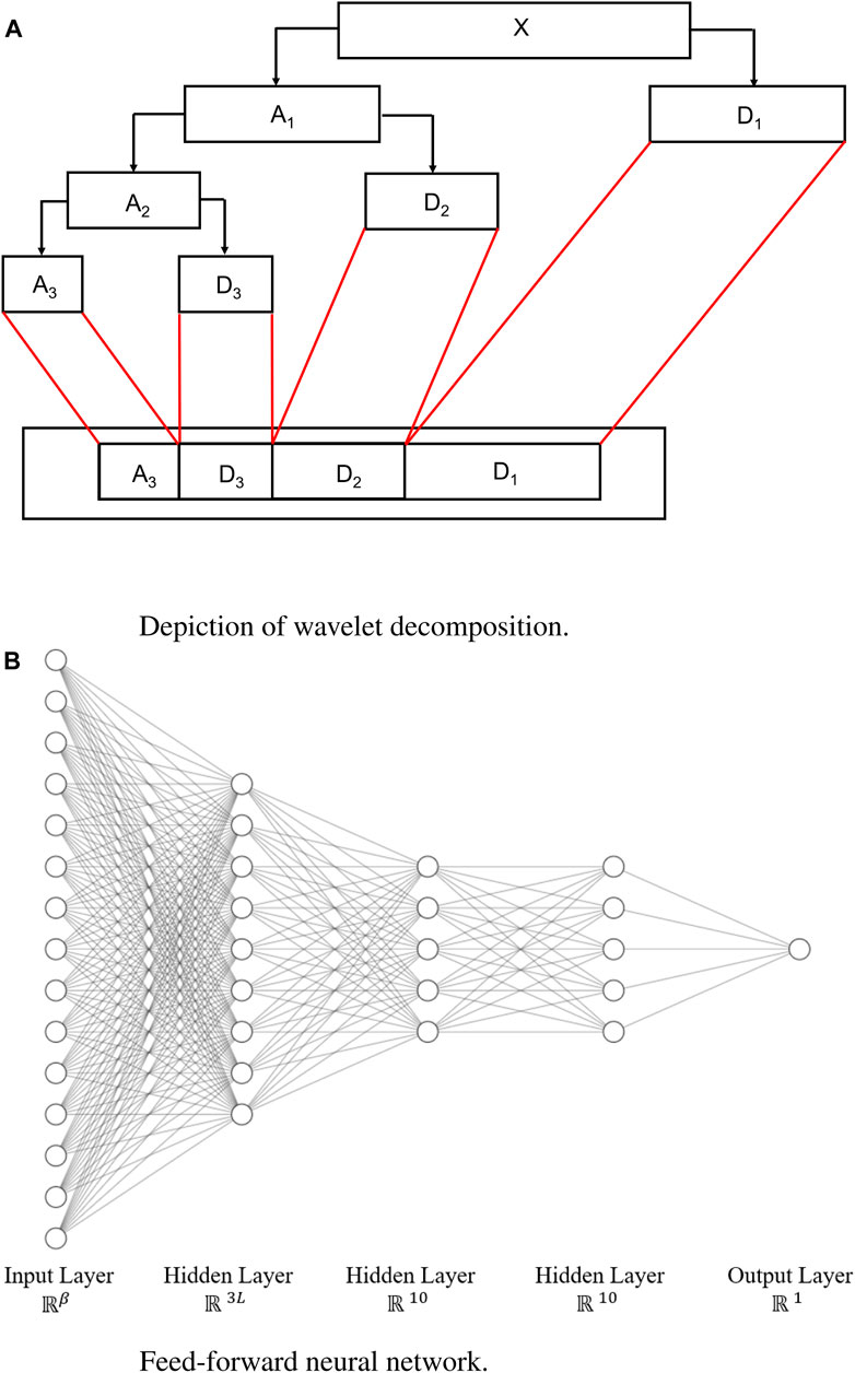
FIGURE 1. Wavelet decomposition and the neural network. (A) Diagram showing wavelet decomposition with k = 3, adapted from Matlab one-dimensional wavelet decomposition documentation (MathWorks, 2023). (B) Neural networks for wind speed and power prediction, where β = Lq (k + 1).

The output of the wavelet decomposition step is a matrix of dimension of n × Lq (k + 1), where q is the number of inputs. For wind speed forecasting, q = 2 because only past wind speed and the derivative of past wind speed are used, whereas for power forecasting, q = 3 as past wind speed, derivative of past wind speed, and past power are used.

3.2 The neural network step

The choice of neural networks here is because deep learning models are quite adept at dealing with nonlinear data and their success in the recent wind forecasting effort does not appear entirely by chance, as we argued in the Introduction section.

For the power prediction model, the response variable, y, is the h-hour ahead original power data, scaled to a range of 0–1. For the forecasting of wind speed, the computation is similar except for the absence of wind power in the input as well as in the response variable. While it is possible to include other environmental variables in the WDNN model, this work restricts predictive variables to wind speed and past power, not only because they have an outsize influence in wind power production (Ding, 2019) but also because wind speed is the commonly available measurements for all wind farms. Other environmental measurements may or may not be available, especially for some small wind farms.

The ANNs used in our algorithm are made up of fully-connected input, three hidden, and output layers as depicted in Figure 1B. The dimensions of the input into the ANNs (i.e., the number of features resulting from the decomposition step) denoted by β, vary depending on the type of prediction to be done—power or speed—and satisfies β = Lq (k + 1). The hidden layers of the ANNs use a Rectified Linear Unit (ReLU) activation function are comprised of 3L, 10, and 10 nodes each, and the output layer uses the sigmoid activation function.

3.3 Choice of the neural network architecture

For time series problems, researchers would tend to go with a neural network that can take previous data points into account during the feedforward process such as RNN or more complex forms of it like LSTM or the Gated Rectilinear Unit (GRU). These methods tend to provide better results in such cases. In this work, however, that is not the case. This is due to the fact that the wavelet decomposition step shuffles the data, consequently nullifying the positive effects that models like RNN, LSTM, and GRU might have. A simple feedforward neural network was deemed sufficient and this work shows that it outperforms the RNN-based and LSTM-based methods in every metric.

The numbers of layers and neurons in these layers were chosen by using a Bayesian optimization algorithm (Snoek et al., 2012), which works by constructing a posterior distribution of functions (Gaussian process) that best describes the function one wants to optimize. As the number of observations grows, the posterior distribution improves, and the algorithm becomes more certain of which regions in parameter space are worth exploring and which are not. This process is designed to minimize the number of steps required to find a combination of parameters that are close to the optimal combination. To do so, this method uses a proxy optimization problem (finding the maximum of the acquisition function) that is computationally cheaper than grid search. It is implemented in the BayesianOptimization Python library (Nogueira, 2014). We call the BayesianOptimization function which gives us the optimized outcome for the neural network design.

3.4 The algorithm

Step-by-step details of the WDNN models for wind power and wind speed are given in Algorithms 1, 2. A demonstrative graph of the WDNN model for power prediction is provided in Figure 2. The graph shows the algorithm working for one turbine. So, for the simplification of notation in this subsection, let all S_j(i), $S_j^{\prime }(i)$ and P_j(i) be S_j, $S_j^{\prime }$ and P_j respectively. It can be observed that the original data series of wind speed (S_t−L+1, …, S_t), $(S_{t-L+1}^{\prime },\dots ,S_t^{\prime })$ and wind power (P_t−L+1, …, P_t) are first decomposed into k + 1 layers. The decomposed components are then inversely decomposed and used as features for the ANN model for predicting the wind power P_t+h at time t + h. For the WDNN model for wind speed prediction, the demonstrative graph will be similar, except for the absence of P_i(j) and the forecast is ${\widehat{S}}_{t+h}$. It is noteworthy that our prediction model is different from models proposed in Catalão et al. (2011) and Wang et al. (2017) in which the prediction values for each decomposed layer are linearly combined to form a forecast for the original series (for which these models assume that decomposed layers are independent). Here, we directly use P_t+h as the response for the ANN model without predicting for each decomposed layer. By doing this we can avoid summing over the prediction errors for each layer. It is also important to know that the ANN model here can potentially capture the correlations between different layers.

FIGURE 2

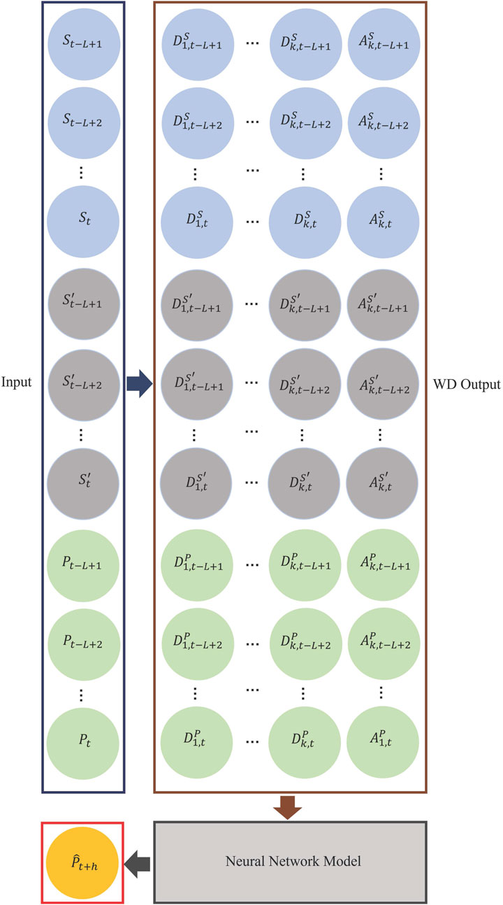
FIGURE 2. WDNN model for wind power forecasting. For wind speed forecasting, the bottom green portion is removed. The forecast becomes ${\widehat{S}}_{t+h}$.

Algorithm 1. WDNN Algorithm for Wind Power.

Require:  Wind speed data (S₁, S₂, …, S_N), first derivative of wind speed data $(S_1^{\prime },S_2^{\prime },\dots ,S_N^{\prime })$, power data (P₁, P₂, …, P_N).

1:   Split the data into training and testing datasets: (S₁, S₂, …, S_T), $(S_1^{\prime },S_2^{\prime },\dots ,S_T^{\prime })$ and (P₁, P₂, …, P_T) as the training set, (S_T+1, S_T+2, …, S_N), $(S_{T+1}^{\prime },S_{T+2}^{\prime },\dots ,S_N^{\prime })$ and (P_T+1, P_T+2, …, P_N) as the testing set.

2:   Specify L, k and h, where

      L = lag,

      k = level of decomposition,

      h = forecasting length.

3:   while i = L: T do

4:    Decompose (S_i−L+1, S_i−L+2, …, S_i), $(S_{i-L+1}^{\prime },S_{i-L+2}^{\prime },\dots ,S_i^{\prime })$ and (P_i−L+1, P_i−L+2, …, P_i) into $({\tilde{A}}_k^S,{\tilde{D}}_k^S,\dots ,{\tilde{D}}_1^S)$, $({\tilde{A}}_k^{S^1},{\tilde{D}}_k^{S^1},\dots ,{\tilde{D}}_1^{S^1})$ and $({\tilde{A}}_k^P,{\tilde{D}}_k^P,\dots ,{\tilde{D}}_1^P)$.

5:    Inversely decompose $({\tilde{A}}_k^S,{\tilde{D}}_k^S,\dots ,{\tilde{D}}_1^S)$, $({\tilde{A}}_k^{S^1},{\tilde{D}}_k^{S^1},\dots ,{\tilde{D}}_1^{S^1})$ and $({\tilde{A}}_k^P,{\tilde{D}}_k^P,\dots ,{\tilde{D}}_1^P)$ as $(A_k^S,D_k^S,\dots ,D_1^S)$ and $(A_k^P,D_k^P,\dots ,D_1^P)$.

6:    Store $(A_k^S,D_k^S,\dots ,D_1^S,A_k^{S^1},D_k^{S^1},\dots ,D_1^{S^1},A_k^P,D_k^P,\dots ,D_1^P)$ as X_i and P_i+h as Y_i.

7:   end while

8:   Train the ANN model using (X_L+1, X_L+2, …, X_T) as training input and (Y_L+1, Y_L+2, …, Y_T) as training outputs.

9:   while i = T + L: N do

10:    Decompose (S_i−L+1, S_i−L+2, …, S_i), $(S_{i-L+1}^{\prime },S_{i-L+2}^{\prime },\dots ,S_i^{\prime })$ and (P_i−L+1, P_i−L+2, …, P_i) into $({\tilde{A}}_k^S,{\tilde{D}}_k^S,\dots ,{\tilde{D}}_1^S)$, $({\tilde{A}}_k^{S^1},{\tilde{D}}_k^{S^1},\dots ,{\tilde{D}}_1^{S^1})$ and $({\tilde{A}}_k^P,{\tilde{D}}_k^P,\dots ,{\tilde{D}}_1^P)$.

11:    Inversely decompose $({\tilde{A}}_k^S,{\tilde{D}}_k^S,\dots ,{\tilde{D}}_1^S)$, $({\tilde{A}}_k^{S^1},{\tilde{D}}_k^{S^1},\dots ,{\tilde{D}}_1^{S^1})$ and $({\tilde{A}}_k^P,{\tilde{D}}_k^P,\dots ,{\tilde{D}}_1^P)$ as $(A_k^S,D_k^S,\dots ,D_1^S)$ and $(A_k^P,D_k^P,\dots ,D_1^P)$.

12:    Store $(A_k^S,D_k^S,\dots ,D_1^S,A_k^{S^1},D_k^{S^1},\dots ,D_1^{S^1},A_k^P,D_k^P,\dots ,D_1^P)$ as X_i and P_i+h as Y_i.

13:   end while

14:   Obtain $({\widehat{Y}}_{T+L},{\widehat{Y}}_{T+L+1},\dots ,{\widehat{Y}}_N)$ by the ANN model using (X_T+L, X_T+L+1, …, X_N) as input.

15:   $MAE=\frac{{\sum }_{i=T+L}^N|\widehat{Y_i}-Y_i|}{N-T-L+1}$

16:   $RMSE=\sqrt{\frac{{\sum }_{i=T+L}^N{(\widehat{Y_i}-Y_i)}^2}{N-T-L+1}}$

17:   return MAE and RMSE

Algorithm 2. WDNN Algorithm for Wind Speed.

Require:  Wind speed data (S₁, S₂, …, S_N), first derivative of wind speed data $(S_1^{\prime },S_2^{\prime },\dots ,S_N^{\prime })$.

1:   Split the data into training and testing datasets: (S₁, S₂, …, S_T) and, $(S_1^{\prime },S_2^{\prime },\dots ,S_T^{\prime })$ as the training set, (S_T+1, S_T+2, …, S_N) and $(S_{T+1}^{\prime },S_{T+2}^{\prime },\dots ,S_N^{\prime })$ as the testing set.

2:   Specify L, k and h, where

      L = lag,

      k = level of decomposition,

      h = forecasting length.

3:   while i = L: T do

4:    Decompose (S_i−L+1, S_i−L+2, …, S_i) and $(S_{i-L+1}^{\prime },S_{i-L+2}^{\prime },\dots ,S_i^{\prime })$ into $({\tilde{A}}_k^S,{\tilde{D}}_k^S,\dots ,{\tilde{D}}_1^S)$ and $({\tilde{A}}_k^{S^1},{\tilde{D}}_k^{S^1},\dots ,{\tilde{D}}_1^{S^1})$.

5:    Inversely decompose $({\tilde{A}}_k^S,{\tilde{D}}_k^S,\dots ,{\tilde{D}}_1^S)$ and $({\tilde{A}}_k^{S^1},{\tilde{D}}_k^{S^1},\dots ,{\tilde{D}}_1^{S^1})$ as $(A_k^S,D_k^S,\dots ,D_1^S)$ and $({\tilde{A}}_k^{S^1},{\tilde{D}}_k^{S^1},\dots ,{\tilde{D}}_1^{S^1})$.

6:    Store $(A_k^S,D_k^S,\dots ,D_1^S,A_k^{S^1},D_k^{S^1},\dots ,D_1^{S^1})$ as X_i and S_i+h as Y_i.

7:   end while

8:   Train the ANN model using (X_L+1, X_L+2, …, X_T) as training input and (Y_L+1, Y_L+2, …, Y_T) as training outputs.

9:   while i = T + L: N do

10:    Decompose (S_i−L+1, S_i−L+2, …, S_i) and $(S_{i-L+1}^{\prime },S_{i-L+2}^{\prime },\dots ,S_i^{\prime })$ into $({\tilde{A}}_k^S,{\tilde{D}}_k^S,\dots ,{\tilde{D}}_1^S)$ and $({\tilde{A}}_k^{S^1},{\tilde{D}}_k^{S^1},\dots ,{\tilde{D}}_1^{S^1})$.

11:    Inversely decompose $({\tilde{A}}_k^S,{\tilde{D}}_k^S,\dots ,{\tilde{D}}_1^S)$ and $({\tilde{A}}_k^{S^1},{\tilde{D}}_k^{S^1},\dots ,{\tilde{D}}_1^{S^1})$ as $(A_k^S,D_k^S,\dots ,D_1^S)$ and $({\tilde{A}}_k^{S^1},{\tilde{D}}_k^{S^1},\dots ,{\tilde{D}}_1^{S^1})$.

12:    Store $(A_k^S,D_k^S,\dots ,D_1^S,A_k^{S^1},D_k^{S^1},\dots ,D_1^{S^1})$ as X_i and S_i+h as Y_i.

13:   end while

14:   Obtain $({\widehat{Y}}_{T+L},{\widehat{Y}}_{T+L+1},\dots ,{\widehat{Y}}_N)$ by the ANN model using (X_T+L, X_T+L+1, …, X_N) as input.

15:   $MAE=\frac{{\sum }_{i=T+L}^N|\widehat{Y_i}-Y_i|}{N-T-L+1}$

16:   $RMSE=\sqrt{\frac{{\sum }_{i=T+L}^N{(\widehat{Y_i}-Y_i)}^2}{N-T-L+1}}$

17:   return MAE and RMSE

4 Analysis and discussion

This section provides the analysis of the WDNN method using three large datasets. We will proceed with explaining the datasets and performance metric used first, followed by an analysis to support the choice of design parameters used in WDNN, and then a study comparing the short-term forecasting performance of WDNN and several alternative methods.

4.1 Datasets

Data from three wind farms is used to test the algorithms. Dataset-1 and Dataset-2 contain wind speed and power information, while Dataset-3 contains only wind speed. All datasets are available through the data/code sharing platform Zenodo. The original Dataset-3 is maintained by the National Renewable Energy Laboratory (NREL), the preprocessed version of Dataset-3 is also shared through the aforementioned Zenodo site.

Due to the fact that these are real datasets, some processing was done to prepare the data for numerical computing. This processing includes the computation of derivatives. Derivatives of wind speed and wind power are computed using the backward differences. So, the derivative F′, of a variable F, at time T, using the backward difference formulation is as shown in Eq. 1.

$F_T^{\prime }=F_T-F_{T-1}(1)$

4.1.1 Dataset-1

Dataset-1 is from an offshore wind farm in Europe. The wind farm houses 36 turbines and a meteorological mast, as shown in Figure 3. The dataset contains 4 years (January 2007-December 2010) of wind speed, power, and other measurements, with an original time resolution of 10 min. For this study, the data is aggregated to an hourly resolution and only wind speed and wind power are used. The first 3 years of data (January 2007-December 2009) is used for training, while the last year (January 2010-December 2010) is used for testing. The minimum and maximum wind speeds are 0.42 m/s and 24.30 m/s, respectively, and wind power ranges between 0 and 1. The total number of observations is 26,241 with 18,293 for training and 8,178 for testing.

FIGURE 3

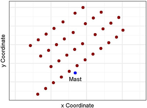
FIGURE 3. Layout of wind turbines used in Dataset-1.

4.1.2 Dataset-2

Dataset-2 is from an onshore wind farm in the United States. The farm contains more than 200 wind turbines and multiple meteorological masts, as shown in Figure 4. Data from 160 turbines is used for this study because the selected data covers a long time range of 34 months (January 2009–October 2011) of wind speed, wind power, and other measurements, with an original time resolution of 10 min. Again, for this study, the data is aggregated to an hourly resolution, and only wind speed and wind power are used. The first 2 years of data (January 2009–December 2010) is used for training, while the last 10 months (January 2011–October 2010) is used for testing. The minimum and maximum wind speeds are 0 m/s and 24.35 m/s respectively, and wind power ranges between 0 and 1. The total number of observations is 22,838 with 15,592 for training and 7,246 for testing.

FIGURE 4

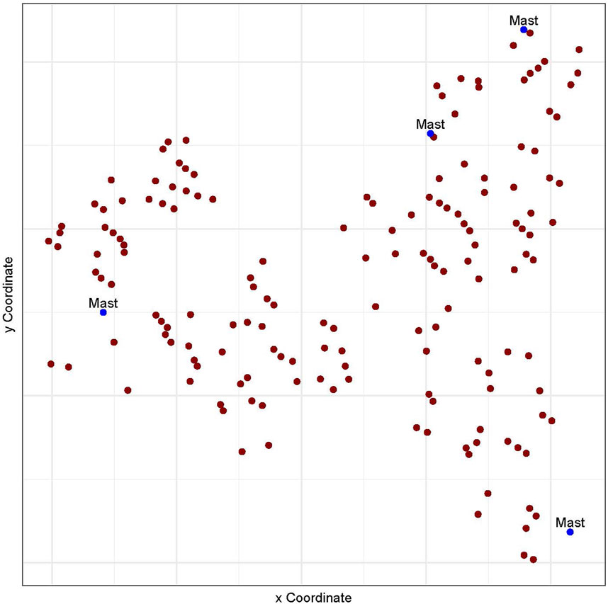
FIGURE 4. Layout of wind turbines used in Dataset-2.

4.1.3 Dataset-3

Dataset-3 has only wind speed data, with no power or other features. It is from a wind farm in Wyoming, United States, and was obtained from datasets made publicly available by NREL. The farm contains 100 wind turbines placed in a 10 × 10 grid, as shown in Figure 5. The Site IDs and coordinates of the vertices of the grid are (867,382, −105.1944°W, 41.87279°N), (877,179, −104.9711°W, 41.89172°N), (867,373, −105.1687°W, 41.70660°N), and (877,170, −104.9461°W, 41.72548°N). The dataset contains 6 years (January 2009–December 2014) of wind speed data with an hourly time resolution. The first 5 years of data (January 2009–December 2013) is used for training, while the last year (January 2014–December 2014) is used for testing. The minimum and maximum wind speeds are 0.01 m/s and 37.46 m/s respectively. The original Dataset-3 can be obtained from the NREL Wind Prospector Website. This option is for single site downloads via a web-interface. The data can also be obtained through the Wind Toolkit API which requires signing up and obtaining a unique API key according to the instructions on the website. The total number of observations is 52,590 with 43,824 for training and 8,766 for testing.

FIGURE 5

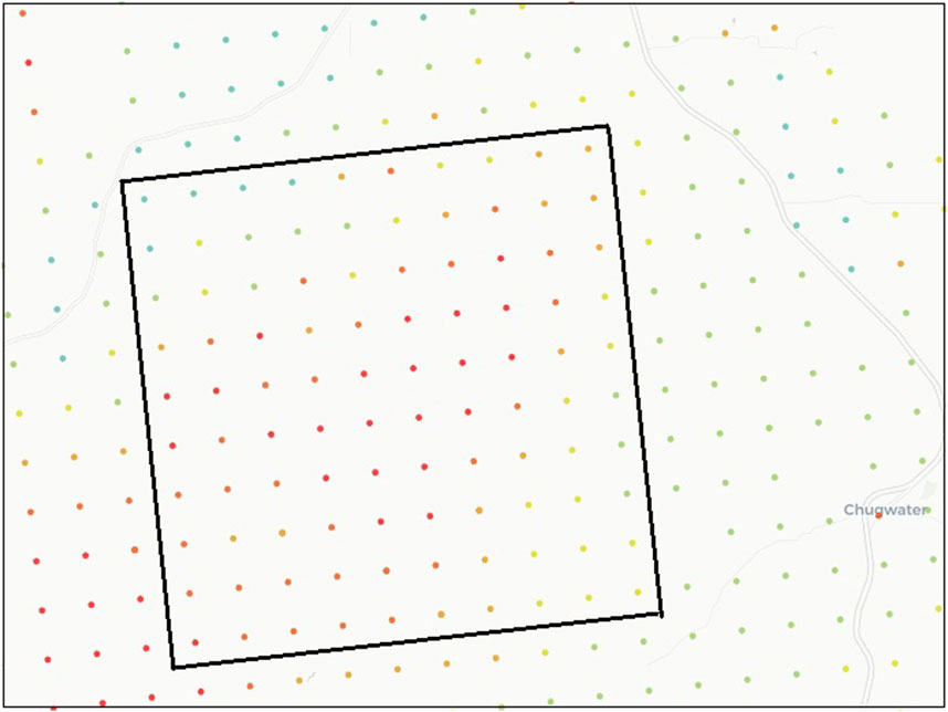
FIGURE 5. The tilted rectangle shows the layout of wind turbines on the 10 × 10 grid used in Dataset-3. Figure credited to the NREL Wind Prospector website (NREL, 2022).

4.2 Evaluation metrics and computational setup

The mean absolute error (MAE) and root mean squared error (RMSE) are the commonly used performance metrics (Ding, 2019, Chapter 2). Both metrics evaluate the performance of a point forecast. Consider a set of n test data points, x_j, j = 1, 2, …, n, the corresponding forecast of each of which is ${\widehat{x}}_j$. Eqs 2, 3 respectively, show how MAE and RMSE are computed for an individual turbine i:

$MA{E}_i=\frac{1}{n}{\displaystyle \sum _{i=j}^n}|{\widehat{x}}_j-x_j|(2)$

$RMS{E}_i=\sqrt{\frac{1}{n}{\displaystyle \sum _{j=1}^n}{\left({\widehat{x}}_j-x_j\right)}^2}.(3)$

For a wind farm containing N_tur turbines, the farm MAE and RMSE are the average of the individual values, i.e., using Eqs 4 and 5 below

$MAE=\frac{1}{N_{\mathit{tur}}}{\displaystyle \sum _{i=1}^{N_{\mathit{tur}}}}MA{E}_i(4)$

$RMSE=\frac{1}{N_{\mathit{tur}}}{\displaystyle \sum _{i=1}^{N_{\mathit{tur}}}}RMS{E}_i.(5)$

These metrics are used, in this work, to evaluate and compare the results of the WDNN models with other models. We mostly present the MAE results to save space. The overall message using either MAE or RMSE is consistent.

All computations were done on two high-performance computing clusters. One cluster had a dual-GPU Tesla K80 accelerators having 128GB RAM with Intel(R) Xeon(R) CPU E5-2680 v4 @ 2.40GHz. The other cluster was a combination of NVIDIA A100 40GB GPUs and NVIDIA RTX6000 24GB GPUs with Intel(R) Xeon(R) Gold 6248R CPU @ 3.00GHz. Both clusters ran on Linux (CentOS 7).

4.3 Sensitivity analysis of model and parameter choices

4.3.1 Wavelet and level of decomposition choices

We have chosen db4 and Level 4 as the default choice in our wavelet decomposition step. Here we conduct a numerical analysis to test how sensitive these choices are.

We vary the choices of the wavelet basis functions and the decomposition levels. We consider a total of ten options from the wavelet families, including Haar, Daubechies (db), Coiflets (coif), Biorthogonal (bior), and Reverse biorthogonal (rbio). For each of the wavelet choice, three decomposition levels, k ∈ {3, 4, 5}, are considered. A subset of Dataset-1 is used for this analysis. To further reduce time, the forecast is made for up to 6 h ahead, i.e., h ∈ {1, 2, …, 6}. The same neural network is used in the subsequent step. Altogether, this analysis runs a total of 30 numerical experiments and makes 180 forecasts.

Table 1 presents the MAE of the 180 forecasting outcomes. A table of RMSE results for this and the other computation can be found in the appendix. The right-most column is the average of all the values obtained from all the decomposition at a certain value of k, whereas the last row is the average of all the values obtained from a particular wavelet. A perusal of the tables reveals the following: (a) the db4 wavelet and k = 4 are the best performing wavelet and decomposition level; and (b) the outcome of WDNN is not sensitive to the two wavelet step-related choices.

TABLE 1

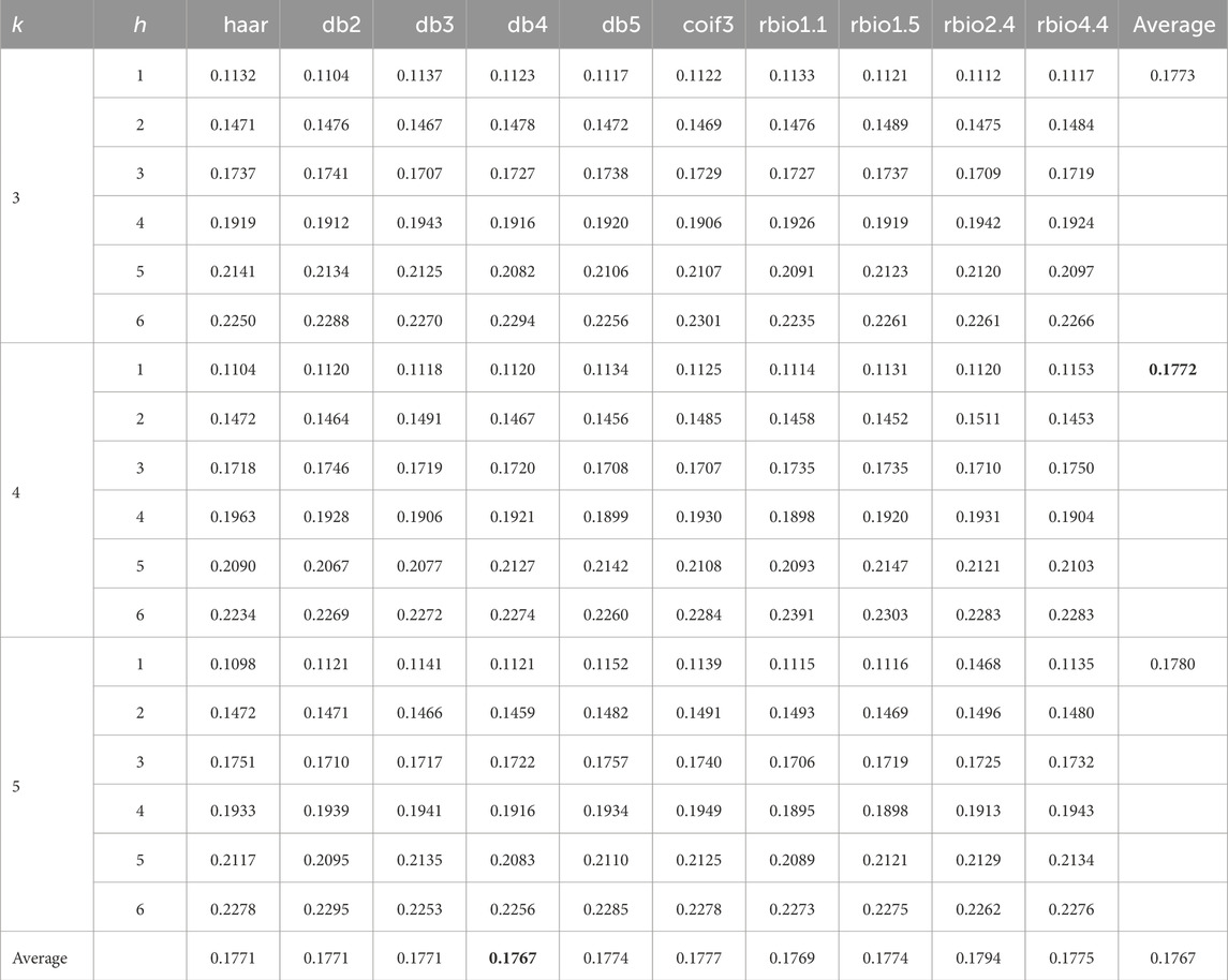
TABLE 1. Performance of different wavelets and levels of decomposition (MAE).

4.3.2 Neural network choice

We further test the choices of the neural network architecture. Despite the popularity of RNN and LSTM in handling time series data, WDNN settles on using a most classical, simple feedforward neural network (FFNN). Earlier, we explained that the reason that FFNN is a better choice because after the wavelet decomposition, the output is not maintained strictly in the original time series order. What this means is that while the original data is time series, the data seen by the neural network model in WDNN is not, so much so, that the advantage for RNN and LSTM no longer exists. Here we present numerical evidence supporting our choice. In this sensitivity analysis, the wavelet choice is set to db4 and the level of decomposition is set to four. Three choices of ANN are studied: FFNN, RNN, and LSTM.

Table 2 shows the MAE results for all three sets of models using Dataset-1. The forecasts are made for up to 12 h. FFNN outperforms RNN and LSTM for all forecasting periods and the last row is the average of all forecasting periods. Similar results are obtained for other datasets and for power prediction as well. For brevity, Tables 3, 4 only present the summary information, i.e., the average of all forecasting periods. Furthermore, Table 5 shows that running FFNN is faster than running RNN and LSTM (for the purpose of illustration, only the run time for 1-h ahead forecast is shown). Compared with RNN, FFNN only takes about one-fifth (or shorter) the time, and compared with LSTM, FFNN’s run time is an order of magnitude shorter.

TABLE 2

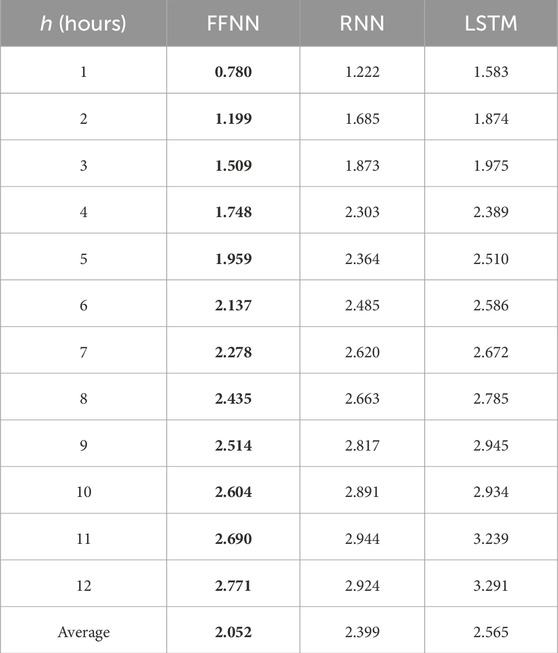
TABLE 2. Performance comparison of different neural networks for wind speed prediction using Dataset-1 (MAE).

TABLE 3

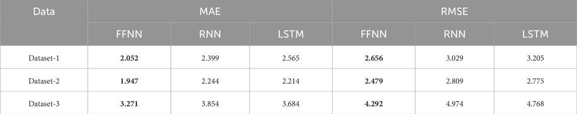
TABLE 3. Performance comparison of different neural networks for wind speed prediction.

TABLE 4

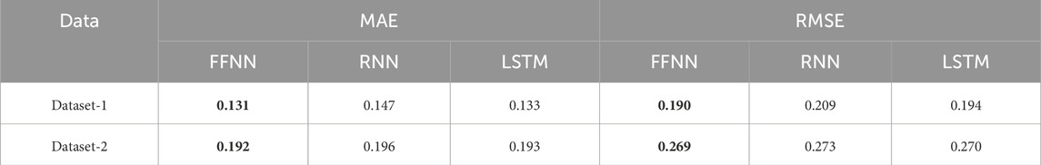
TABLE 4. Performance comparison of different neural networks for wind power prediction.

TABLE 5

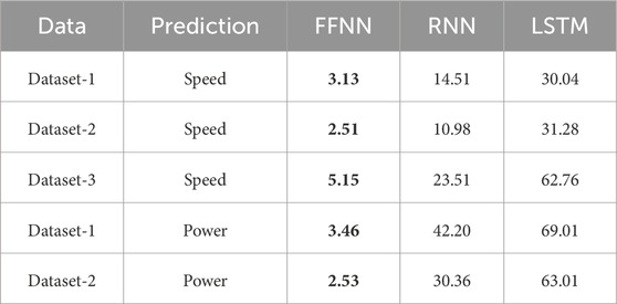
TABLE 5. Run time in minutes for WDNN for h = 1 hour using different networks.

4.4 Comparisons and analysis

In this subsection, we conduct comparison studies for both wind speed forecast and wind power forecast. For wind speed forecast, all three datasets are used, whereas for wind power forecast, only are Dataset-1 and Dataset-2 used, because there are no wind power measurements in Dataset-3.

4.4.1 Methods in comparison

We primarily compare WDNN with other deep learning based methods. The analysis of non-deep learning methods is rather extensive and it is difficult to repeat them. More importantly, the recent trend seems to indicate that deep learning methods generally outperform the non-deep learning, statistical or machine learning methods. For this reason, it makes sense to focus our comparisons with the deep learning methods.

Comparison with deep learning methods is a challenge in and by itself. As we explained in Section 1, there are many variants of deep learning methods but it is not easy to understand how/why each works and it is difficult to replicate the methods/results unless the original authors shared their code. After much effort (over nearly 2 years), we came across three deep learning methods, for which either the code is shared or we have a reasonable reconstruction of the method ourselves. Based on our reading of the literature, these methods also present different varieties of existing deep learning methods; that is a good aspect to be aware of. Next we will briefly explain each of the methods.

The first Deep Forecast (DF) (Ghaderi et al., 2017) is a deep learning-based method that models the spatiotemporal information by a graph whose nodes are data generating entities and whose edges model how these nodes interact with each other. It employs the LSTM neural networks and its output is wind speed predictions. The author of this method provided computer code for reproducing their work.

Spatiotemporal Attention Network (STAN) (Fu et al., 2019) is a framework for forecasting that captures spatial correlations among wind farms and temporal dependencies of the time series. It employs a multi-head self-attention mechanism to extract spatial correlations among wind farms and captures temporal dependencies by a Sequence-to-Sequence (Seq2Seq) model with a global attention mechanism (Fu et al., 2019). STAN’s output is also wind speed predictions. Unable to find code for STAN, we implemented the method ourselves.

Predictive Spatio-temporal Network (PSTN) (Zhu et al., 2019) is a unified framework integrating a CNN and a LSTM for wind speed forecasting. The spatial features are extracted from the spatial wind speed matrices by the CNN at the bottom of the model, the LSTM captures the temporal dependencies among the spatial features extracted from contiguous time points, and, the predicted wind speeds are obtained by the last state of the top layer of the LSTM, which are generated by using the spatial features and temporal dependencies (Zhu et al., 2019). Unlike the other methods already mentioned, however, PSTN works for turbines placed in a rectangular grid, primarily because of the use of CNN for capturing the spatial features. As a consequence, this model is only applied on Dataset-3, as it is the only dataset that meets that requirement. Unable to find code for PSTN, we implemented the method ourselves.

In addition to the three deep-learning methods, we also included in the comparison the so-called persistence (Per) forecasting model (Ding, 2019, Chapter 2), which is arguably the simplest method used and still in many cases an industrial benchmark standard. The persistence model can be applied to wind speed as well as to wind power. It takes the most recent observation of either wind speed or wind power and uses it as is for whichever forecast, i.e., for any hours ahead. The persistence model can be advantageous and robust for ultra short-term forecasting, like in a few minutes. It is not easy to outperform the persistence method under the ultra short-term circumstances, but the persistence model loses its steam when the forecast goes more than 1 h. Considering the simplicity of the persistent model, any new forecasting method failing to outperform the persistence model simply does not have the attraction at all for practitioners to consider or adopt.

WDNN is implemented in Python using PyWavelets (Lee et al., 2019) and TensorFlow (Abadi et al., 2016) with GPU acceleration. Lag is set to L = 6, the level of decomposition is set to k = 4 and the forecasting length, h ∈ {1, 2, …, 12}. The MAE is used as the loss function for ANNs, with the Root Mean Squared Propagation (RMSProp) extension to the gradient descent optimization algorithm as an optimizer with a learning rate of 0.001. The maximum number of training epochs is 500, with early stopping implemented to prevent over-fitting (Géron, 2019, Chapter 4). STAN and PSTN are implemented in Python using PyTorch (Paszke et al., 2019) following the algorithms described in Fu et al. (2019) and Zhu et al. (2019) respectively.

4.4.2 Wind speed forecasting

All three datasets are used for wind speed forecasting. The forecasting horizon is set to be up to 12 h ahead, consistent with the duration used in Ding (2019). The rationale is that for more than 12 h, it is rarely that one can obtain advantageous forecasting results using purely data-driven methods.

Tables 6–8 present the outcome of the comparison. For Dataset-1 and Dataset-2, the comparison includes Per, DF, STAN, and WDNN, whereas for Dataset-3, the comparison includes all above plus PSTN. The results show that WDNN outperforms all other models except for PSTN.

TABLE 6

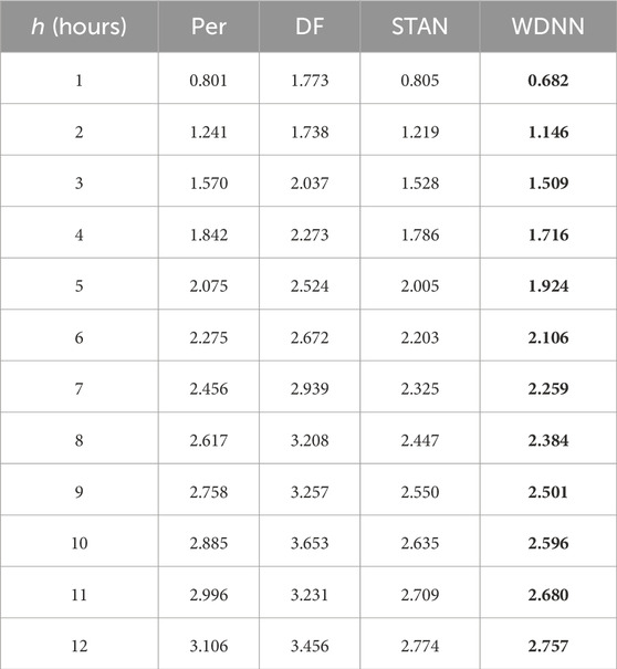
TABLE 6. Comparison of different models for wind speed prediction using Dataset-1 (MAE).

TABLE 7

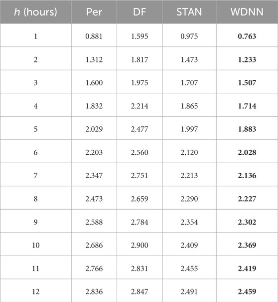
TABLE 7. Comparison of different models for wind speed prediction using Dataset-2 (MAE).

TABLE 8

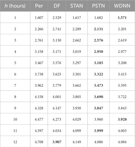
TABLE 8. Comparison of different models for wind speed prediction using Dataset-3 (MAE).

While PSTN does better in Dataset-3, we would like to note the following points: (a) the differences between PSTN and WDNN are rather close. PSTN outperforms WDNN generally less than 2%. But running PSTN is much time consuming. A simple test shows that to train PSTN, it takes 17.25 min where as under the same setting, training WDNN takes only 3.13 min. (b) The advantage of PSTN is not easy to generalize. This can be attributed to the fact that PSTN is designed specifically for a scenario such as this, where the turbines are laid out in a square grid, as it captures spatial relationships between the turbines. This requirement limits the practical use of the method, as square grid are not the layout of choice for the vast majority of wind farms across the world. By contrast, none of the other methods including WDNN requires such strict layout.

We further observe that the DF results become somewhat unstable after h = 8. In principle the MAE and RSME should monotonically increase. However, this is not the case for DF. More than this shortcoming, DF’s performance is not impressive and generally worse than the persistence model; this renders DF less practically appealing. STAN, on the other hand, delivers a competitive outcome, mostly outperforming the persistence model. But STAN’s performances for shorter hours, like h = 1 or 2 are worse than the persistence model for both Dataset-2 and Dataset-3. Overall, STAN’s performance lags behind WDNN by 1.5% for Dataset-1, 4.2% for Dataset-2, and 2.0% for Dataset-3, and its under-performance can be as large as 13.5%.

4.4.3 Wind power forecasting

This subsection presents the analysis of wind power forecasting. Because Dataset-3 does not have power, it is excluded from the analysis in this subsection. Also because PSTN is only applicable on Dataset-3 due to its intrinsic design, it is not included in the power forecast analysis either.

When it comes to wind power prediction, there are two ways in which wind power can be predicted—directly or indirectly. The direct way is to use whatever inputs, past observed wind speed and/or wind power to directly forecast the future wind power. The indirect way is a two-step method that involves wind speed prediction step, and then use the power curve to compute the forecasted power based on the predicted wind speed. WDNN has two versions, it can predict a speed first or it can directly predict wind power.

The persistence model can be directly used for wind power prediction. When “Per” appears in the subsequent tables, it means the application of persistence directly on power (without the wind speed information involved at all).

If one applies the persistence model to wind speed and produces wind speed forecasts, one needs to use a power curve model to covert the speed forecast to power. A power curve model is needed not only for the wind speed-based persistence, but also for DF and STAN, because they produce wind speed forecasts not wind power forecasts. For the version of WDNN predicting the wind speed first, it needs the power curve model.

We in this subsection therefore consider two power curve models. One is known as the binning method based on the IEC standard 61400-12 (International Electrotechnical Commission IEC, 2017), a simple method commonly used in the wind industry. Ding (2019, Chapter 5) analyzes a large group of machine learning-based power curve models, including k-Nearest Neighbors, kernel method, spline-based method, Bayesian tree-based method, and support vector machine. It was then identified that the hybrid kernel method known as the Additive Multiplicative Kernel (AMK) (Lee et al., 2015) produced the best performance then, but AMK is outperformed by a most recent development of the TempGP method (Prakash et al., 2023). For this reason, the second choice of power curve we use is the TempGP.

The binning method is only used together with the wind speed-based persistence model. When the acronym “Bin” appears in the following comparison tables, it means just this combination. The two options, Per and Bin, are the baseline benchmarks, as they are arguably the simplest numerical methods used for making wind power forecast. As explained before, if a new method does not outperform either of these baselines, its practical relevance is then seriously called into questions.

For DF, STAN, and WDNN producing wind speed forecasting, they are paired with TempGP to make the best use of the existing power curve models. They are labeled as DF-TGP, STAN-TGP and WDNN(s)-TGP, respectively. WDNN directly producing wind power forecasts is labeled as WDNN(p).

Tables 9, 10 present the comparison results of wind power forecast. WDNN outperforms other models for all forecast periods in Dataset-1. In Dataset-2 WDNN outperforms other models for most of the forecast periods, but in a few areas, DF produces a better result. The merit of DF, however, is not strong, for the following reasons. The first is that DF does not seem to produce a competitive results for h shorter than 8 h. Under those forecasting time horizons, DF is generally worse than the two baselines. The second is the relative instability of DF for h bigger—this is where DF outperforms other methods. While other methods generally have a monotonic degradation on performance as h increases, DF’s trend is more complicated and less predictable when h goes beyond certain value. This strange behavior renders DF less desirable in practice. STAN performs well overall, but is generally worse than WDNN. While WDNN and STAN’s performances are close on Dataset-2, WDNN’s advantage margin over STAN is rather pronounced.

TABLE 9

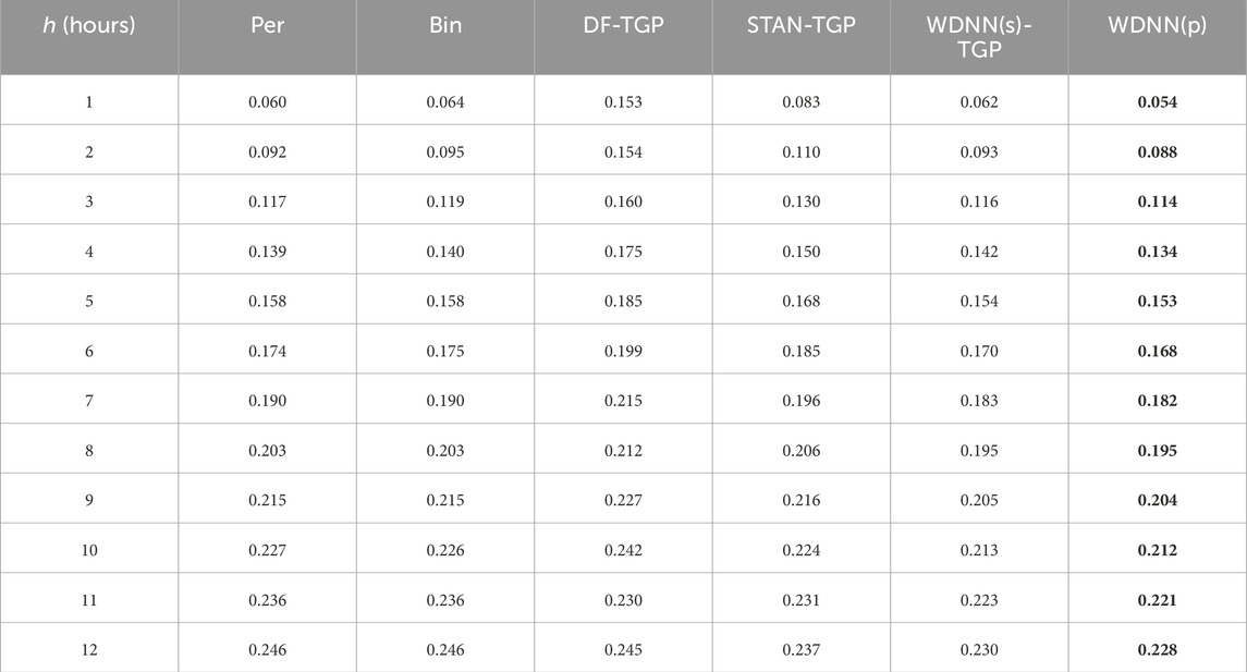
TABLE 9. Comparison of different models for wind power prediction using Dataset-1 (MAE).

TABLE 10

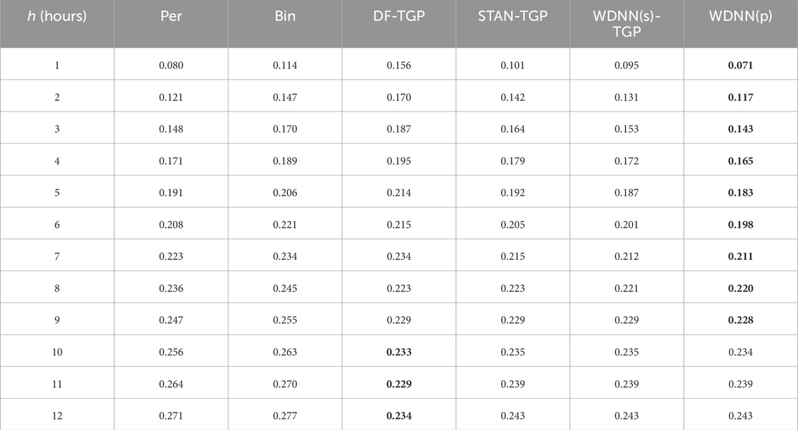
TABLE 10. Comparison of different models for wind power prediction using Dataset-2 (MAE).

5 Conclusion

This work introduces WDNN, a novel coupling of wavelet decomposition ideas and deep learning, yielding a method that can predict wind speed as an intermediate step to the prediction of produced power, or predict power produced directly. It is worth pointing out that both parts of the algorithm—wavelet decomposition and neural network—are easy to implement and computationally inexpensive. Furthermore, WDNN is agnostic to the wind farm layout, which is an important point, as the only model to outperform the WDNN is constrained to working on wind farms whose turbines are laid out in an orthogonal grid. WDNN models can also work as well for a single turbine as they can for a collection of turbines or a whole wind farm. WDNN predictions are stable, without some of the questionable results that were noticed from another model in the case studies.

While the power of deep learning, for simple as well as complex problems, is well documented, scientists and engineers use transforms such as wavelet decomposition routinely to good effect. The success of WDNN puts into sharp relief the utility of wavelet decomposition as a tool for feature engineering/data transformation in the wind power forecasting space.

A couple of ideas are immediately apparent. Firstly, with an effective algorithm for dealing with the data, the machine learning model that it is fed into does not have to be complex. The use of a simple feedforward neural network in WDNN buttresses this fact. Secondly, the possible use of other environmental variables is made easy by WDNN’s design. Thirdly, another area to look at would be taking the spatial relationships between the turbines into account in the model, as PSTN does, but not limiting to a rigid grid. This, in theory, should make the model more competitive.

There is something to be said for the use of multiple and diverse datasets in putting a method such as WDNN through its paces. Although it is possible to use a single dataset with a few turbines, as is the case with many studies of this kind, the use of a variety of datasets, as is done here, enables the reader to assess if the method is effective regardless of the particular circumstances of a wind farm. This lends more credibility to the method. As readers see in our comprehensive case studies, the performance outcomes are complex when methods are used and compared on hundreds of turbines and multiple wind farms. A claim of strict superiority is often not credible, so it is best for us to acknowledge the real-life complexity.

Speaking of future work, first of all, all we deal with here is time series data for a specific turbine. In reality many turbines co-exist on a wind farm and produce spatio-temporal datasets. It is of great interest to see how effectively the data from neighboring turbines can be used for improving the accuracy of the forecast. The approach of finding the so-called informative neighborhood, as first proposed in Pourhabib et al. (2016), is worth a serious look and further research. Another area of improvement is as follows. As one can see from this study, the performance improvement the proposed method makes is more pronounced for 1-h or 2-h ahead forecast, but less impressive for 12-h ahead forecast. It will be important to understand the fundamental reasons behind such performance differences and thus devise effective strategies to extend the improvement from the very short terms to moderate short terms like 12- to 24-h ahead.

Data availability statement

Publicly available datasets were analyzed in this study. This data can be found here: https://zenodo.org/record/7699252.

Author contributions

AK: Conceptualization, Data curation, Formal Analysis, Investigation, Methodology, Validation, Visualization, Writing–original draft. JX: Conceptualization, Investigation, Methodology, Writing–review and editing. NG: Conceptualization, Methodology, Resources, Supervision, Writing–review and editing. YD: Conceptualization, Funding acquisition, Investigation, Methodology, Resources, Supervision, Writing–review and editing.

Funding

The author(s) declare financial support was received for the research, authorship, and/or publication of this article. AK and YD were partially supported by NSF grant IIS-1741173l.

Conflict of interest

The authors declare that the research was conducted in the absence of any commercial or financial relationships that could be construed as a potential conflict of interest.

Publisher’s note

All claims expressed in this article are solely those of the authors and do not necessarily represent those of their affiliated organizations, or those of the publisher, the editors and the reviewers. Any product that may be evaluated in this article, or claim that may be made by its manufacturer, is not guaranteed or endorsed by the publisher.

References

Abadi, M., Agarwal, A., Barham, P., Brevdo, E., Chen, Z., Citro, C., et al. (2016). TensorFlow: large-scale machine learning on heterogeneous systems. arXiv preprint arXiv:1603.04467.

Google Scholar

Box, G. E., Jenkins, G. M., Reinsel, G. C., and Ljung, G. M. (2015). Time series analysis: forecasting and control. Hoboken, NJ: John Wiley and Sons.

Google Scholar

Cadenas, E., and Rivera, W. (2010). Wind speed forecasting in three different regions of Mexico, using a hybrid ARIMA–ANN model. Renew. Energy 35, 2732–2738. doi:10.1016/j.renene.2010.04.022

CrossRef Full Text | Google Scholar

Calif, R., and Schmitt, F. G. (2012). Modeling of atmospheric wind speed sequence using a lognormal continuous stochastic equation. J. Wind Eng. Industrial Aerodynamics 109, 1–8. doi:10.1016/j.jweia.2012.06.002

CrossRef Full Text | Google Scholar

Catalão, J. P. S., Pousinho, H. M. I., and Mendes, V. M. F. (2011). Short-term wind power forecasting in Portugal by neural networks and wavelet transform. Renew. Energy 36, 1245–1251. doi:10.1016/j.renene.2010.09.016

CrossRef Full Text | Google Scholar

Center, B. P. (2020). Annual energy outlook 2020, 12. Washington, DC: Energy Information Administration, 1672–1679.

Google Scholar

Chang, W.-Y. (2014). A literature review of wind forecasting methods. J. Power Energy Eng. 2, 161–168. doi:10.4236/jpee.2014.24023

CrossRef Full Text | Google Scholar

Chen, N., Qian, Z., and Meng, X. (2013). Multistep wind speed forecasting based on wavelet and Gaussian processes. Math. Problems Eng. 2013, 1–8. doi:10.1155/2013/461983

CrossRef Full Text | Google Scholar

Cleveland, R. B., Cleveland, W. S., McRae, J. E., and Terpenning, I. (1990). STL: a seasonal-trend decomposition. J. Official Statistics 6, 3–73.

Google Scholar

Daubechies, I. (1988). Orthonormal bases of compactly supported wavelets. Commun. Pure Appl. Math. 41, 909–996. doi:10.1002/cpa.3160410705

CrossRef Full Text | Google Scholar

Daubechies, I. (1992). Ten Lectures on wavelets (SIAM)

Google Scholar

Ding, Y. (2019). Data science for wind energy. Boca Raton, FL: Chapman and Hall/CRC Press.

Google Scholar

Dowell, J., and Pinson, P. (2015). Very-short-term probabilistic wind power forecasts by sparse vector autoregression. IEEE Trans. Smart Grid 7, 763–770.

CrossRef Full Text | Google Scholar

Dragomiretskiy, K., and Zosso, D. (2013). Variational mode decomposition. IEEE Trans. Signal Process. 62, 531–544. doi:10.1109/tsp.2013.2288675

CrossRef Full Text | Google Scholar

Erdem, E., and Shi, J. (2011). ARMA based approaches for forecasting the tuple of wind speed and direction. Appl. Energy 88, 1405–1414. doi:10.1016/j.apenergy.2010.10.031

CrossRef Full Text | Google Scholar

Ezzat, A. A., Jun, M., and Ding, Y. (2018). Spatio-temporal asymmetry of local wind fields and its impact on short-term wind forecasting. IEEE Trans. Sustain. Energy 9, 1437–1447. doi:10.1109/tste.2018.2789685

PubMed Abstract | CrossRef Full Text | Google Scholar

Ezzat, A. A., Jun, M., and Ding, Y. (2019). Spatio-temporal short-term wind forecast: a calibrated regime-switching method. Ann. Appl. Statistics 13, 1484–1510. doi:10.1214/19-aoas1243

PubMed Abstract | CrossRef Full Text | Google Scholar

Fu, X., Gao, F., Wu, J., Wei, X., and Duan, F. (2019). “Spatiotemporal attention networks for wind power forecasting,” in 2019 International Conference on Data Mining Workshops (ICDMW) (IEEE), 149–154.

CrossRef Full Text | Google Scholar

Gangwar, S., Bali, V., and Kumar, A. (2020). Comparative analysis of wind speed forecasting using LSTM and SVM. EAI Endorsed Trans. Scalable Inf. Syst. 7, e1.

Google Scholar

Géron, A. (2019). Hands-on machine learning with scikit-learn, keras, and TensorFlow: concepts, tools, and techniques to build intelligent systems. Sebastopol, CA: O’Reilly Media, Inc.

Google Scholar

Ghaderi, A., Sanandaji, B. M., and Ghaderi, F. (2017). Deep forecast: deep learning-based spatio-temporal forecasting. arXiv preprint arXiv:1707.08110.

Google Scholar

Guo, Z., Zhao, W., Lu, H., and Wang, J. (2012). Multi-step forecasting for wind speed using a modified EMD-based artificial neural network model. Renew. Energy 37, 241–249. doi:10.1016/j.renene.2011.06.023

CrossRef Full Text | Google Scholar

Guyon, I., Gunn, S., Nikravesh, M., and Zadeh, L. A. (2008). Feature extraction: foundations and applications. Springer.

Google Scholar

Huang, N. E., Shen, Z., Long, S. R., Wu, M. C., Shih, H. H., Zheng, Q., et al. (1998). The empirical mode decomposition and the hilbert spectrum for nonlinear and non-stationary time series analysis. Proc. R. Soc. Lond. A Math. Phys. Eng. Sci. 454, 903–995. doi:10.1098/rspa.1998.0193

CrossRef Full Text | Google Scholar

International Electrotechnical Commission (IEC) (2017). Iec TS 61400-12-1 ed. 2, wind turbines – Part 12-1: power performance measurements of electricity producing wind turbines. Geneva, Switzerland: IEC.

Google Scholar

Jafarzadeh, S., Fadali, S., Evrenosoglu, C. Y., and Livani, H. (2010). “Hour-ahead wind power prediction for power systems using hidden Markov models and Viterbi algorithm,” in IEEE PES General Meeting (IEEE), 1–6.

CrossRef Full Text | Google Scholar

Kimura, R. (2002). Numerical weather prediction. J. Wind Eng. Industrial Aerodynamics 90, 1403–1414. doi:10.1016/s0167-6105(02)00261-1

CrossRef Full Text | Google Scholar

Kwon, S., Xu, Y., and Gautam, N. (2015). Meeting inelastic demand in systems with storage and renewable sources. IEEE Trans. Smart Grid 8, 1619–1629. doi:10.1109/tsg.2015.2494874

CrossRef Full Text | Google Scholar

Lee, G., Ding, Y., Xie, L., and Genton, M. G. (2015). A kernel plus method for quantifying wind turbine performance upgrades. Wind Energy 18, 1207–1219. doi:10.1002/we.1755

CrossRef Full Text | Google Scholar

Lee, G., Gommers, R., Waselewski, F., Wohlfahrt, K., and O’Leary, A. (2019). Pywavelets: a python package for wavelet analysis. J. Open Source Softw. 4, 1237. doi:10.21105/joss.01237

CrossRef Full Text | Google Scholar

Liu, H., Chen, C., Tian, H.-Q., and Li, Y.-F. (2012). A hybrid model for wind speed prediction using empirical mode decomposition and artificial neural networks. Renew. Energy 48, 545–556. doi:10.1016/j.renene.2012.06.012

CrossRef Full Text | Google Scholar

Liu, H., Tian, H.-Q., Chen, C., and Li, Y.-F. (2010). A hybrid statistical method to predict wind speed and wind power. Renew. Energy 35, 1857–1861. doi:10.1016/j.renene.2009.12.011

CrossRef Full Text | Google Scholar

Liu, Y., Guan, L., Hou, C., Han, H., Liu, Z., Sun, Y., et al. (2019). Wind power short-term prediction based on LSTM and discrete wavelet transform. Appl. Sci. 9, 1108. doi:10.3390/app9061108

CrossRef Full Text | Google Scholar

Mallat, S. G. (1989). A theory for multiresolution signal decomposition: the wavelet representation. IEEE Trans. Pattern Analysis Mach. Intell. 11, 674–693. doi:10.1109/34.192463

CrossRef Full Text | Google Scholar

MathWorks (2022). Analyze signals and images in the wavelet domain.

Google Scholar

MathWorks (2023). Wavedec: 1-d wavelet decomposition

Google Scholar

Mohandes, M. A., Halawani, T. O., Rehman, S., and Hussain, A. A. (2004). Support vector machines for wind speed prediction. Renew. Energy 29, 939–947. doi:10.1016/j.renene.2003.11.009

CrossRef Full Text | Google Scholar

More, A., and Deo, M. (2003). Forecasting wind with neural networks. Mar. Struct. 16, 35–49. doi:10.1016/s0951-8339(02)00053-9

CrossRef Full Text | Google Scholar

Nedaei, M., Assareh, E., and Walsh, P. R. (2018). A comprehensive evaluation of the wind resource characteristics to investigate the short term penetration of regional wind power based on different probability statistical methods. Renew. Energy 128, 362–374. doi:10.1016/j.renene.2018.05.077

CrossRef Full Text | Google Scholar

Nogueira, F. (2014). Bayesian Optimization: open source constrained global optimization tool for Python.

Google Scholar

NREL (2022). Wind prospector website.

Google Scholar

Paszke, A., Gross, S., Massa, F., Lerer, A., Bradbury, J., Chanan, G., et al. (2019). Pytorch: an imperative style, high-performance deep learning library. Adv. Neural Inf. Process. Syst. 32, 8024–8035.

Google Scholar

Peng, X., Li, Y., Dong, L., Cheng, K., Wang, H., Xu, Q., et al. (2021). Short-term wind power prediction based on wavelet feature arrangement and convolutional neural networks deep learning. IEEE Trans. Industry Appl. 57, 6375–6384. doi:10.1109/tia.2021.3106887

CrossRef Full Text | Google Scholar

Pourhabib, A., Huang, J. Z., and Ding, Y. (2016). Short-term wind speed forecast using measurements from multiple turbines in a wind farm. Technometrics 58, 138–147. doi:10.1080/00401706.2014.988291

CrossRef Full Text | Google Scholar

Prakash, A., Tuo, R., and Ding, Y. (2023). The temporal overfitting problem with applications in wind power curve modeling. Technometrics 65, 70–82. doi:10.1080/00401706.2022.2069158

CrossRef Full Text | Google Scholar

Reis, A. R., and Da Silva, A. A. (2005). Feature extraction via multiresolution analysis for short-term load forecasting. IEEE Trans. Power Syst. 20, 189–198. doi:10.1109/tpwrs.2004.840380

CrossRef Full Text | Google Scholar

Rumelhart, D. E., Hinton, G. E., and Williams, R. J. (1986). Learning representations by back-propagating errors. Nature 323, 533–536. doi:10.1038/323533a0

CrossRef Full Text | Google Scholar

Schmidhuber, J., and Hochreiter, S. (1997). Long short-term memory. Neural Comput. 9, 1735–1780. doi:10.1162/neco.1997.9.8.1735

PubMed Abstract | CrossRef Full Text | Google Scholar

Snoek, J., Larochelle, H., and Adams, R. P. (2012). Practical Bayesian optimization of machine learning algorithms. Adv. Neural Inf. Process. Syst. 25, 2951–2959.

Google Scholar

Wang, D., Luo, H., Grunder, O., and Lin, Y. (2017). Multi-step ahead wind speed forecasting using an improved wavelet neural network combining variational mode decomposition and phase space reconstruction. Renew. Energy 113, 1345–1358. doi:10.1016/j.renene.2017.06.095

CrossRef Full Text | Google Scholar

Wang, J., Niu, T., Lu, H., Yang, W., and Du, P. (2019). A novel framework of reservoir computing for deterministic and probabilistic wind power forecasting. IEEE Trans. Sustain. Energy 11, 337–349. doi:10.1109/tste.2019.2890875

CrossRef Full Text | Google Scholar

Wang, J., Zhou, Q., Jiang, H., and Hou, R. (2015). Short-term wind speed forecasting using support vector regression optimized by cuckoo optimization algorithm. Math. Problems Eng. 2015, 1–13. doi:10.1155/2015/619178

CrossRef Full Text | Google Scholar

Witherspoon, S., and Fadrhonc, W. (2019). Machine learning can boost the value of wind energy.

Google Scholar

Zhang, Y., Yang, S., Guo, Z., Guo, Y., and Zhao, J. (2019). Wind speed forecasting based on wavelet decomposition and wavelet neural networks optimized by the cuckoo search algorithm. Atmos. Ocean. Sci. Lett. 12, 107–115. doi:10.1080/16742834.2019.1569455

CrossRef Full Text | Google Scholar

Zhu, Q., Chen, J., Shi, D., Zhu, L., Bai, X., Duan, X., et al. (2019). Learning temporal and spatial correlations jointly: a unified framework for wind speed prediction. IEEE Trans. Sustain. Energy 11, 509–523. doi:10.1109/tste.2019.2897136

CrossRef Full Text | Google Scholar

Nomenclature