Thermal field reconstruction and compressive sensing using proper orthogonal decomposition

1 Introduction

Fluid flows and scalar transport are ubiquitous in nature and engineering. Consequently, accurate modeling of flow behavior is important for obtaining a deeper understanding of natural systems and optimizing the design of engineering systems. At a fundamental level, fluid flows are computationally irreducible problems. They are composed of a near-infinite number of particles, each with its own position and velocity at every instant in time. This means that the complete characterization of any flow is impossible for computationally bounded observers (Wolfram, 2023). Furthermore, even if a complete snapshot in time were available, it would be impossible to predict the state at any future time without running a complete simulation of every interaction. Throughout the first half of the 19th century Navier and Stokes developed their famous system of equations that model fluid flows quite well (Panton, 2013). These equations along with the energy equation model the velocity, pressure, temperature, and concentration fields in a fluid and provide a continuous, macroscopic representation of the microscopic process underneath. However, no general, analytical solution exists for these equations, so in many engineering applications today approximate solutions are numerically evaluated. These methods are both computationally expensive and they generate a large amount of data which is difficult to distill for understanding or design purposes.

The study of coherent structures in time-varying flows emerged in the latter half of the 20th century as an attempt to simplify the analysis of chaotic, unpredictable flows (Lumley, 1981). Coherent structures emerge from the interaction between a flowing fluid and the physical boundaries the fluid encounters. Structures leave their mark on the flow, influencing its evolution over space and time. Proper orthogonal decomposition (POD) is an analytical technique developed by Lumley in 1967 that provides a framework for extracting and analyzing these coherent structures (Sirovich, 1987). This technique appears to have been developed independently in several contexts and has also been called the Karhunen-Loeve expansion or principle component analysis. Sirovich further developed this technique, pioneering the “method of snapshots” which takes snapshots of the fluid field as inputs and produces modes forming an orthogonal basis for the flow (Sirovich, 1987; Sirovich and Park, 1990).

Since its inception, POD has been refined and extended. It has been applied to create reduced-order, computationally efficient models of many different aspects of engineering systems in fields such as fluid mechanics, heat transfer, neutronics, and meteorology. Buchan et al. developed a POD based, reduced-order model to simplify neutron flux calculations in nuclear reactors (Buchan et al., 2013). They achieved a reduction in computation time of between 87% and 99%. Epps and Krivitzky studied the effects of noisy data on POD models of velocity in fluid flows, considering the relation between noise level and the singular values derived in the model (Epps and Krivitzky, 2019). Cohen et al. applied POD to the compressive sensing and reconstruction of velocity fields from oscillatory flow over a cylinder. They suggested a potential method to determine sensor placement (Cohen et al., 2003). Raiola et al. studied the effectiveness of such POD reconstruction techniques on the vorticity field of a turbulent flow. They demonstrated the effectiveness of the technique even when the training data has a level of Gaussian noise applied, as is the case in real sensed data (Raiola et al., 2015). Liu et al. used POD to study the coherent turbulent structures in simulated data of wind moving over a city. They developed modes corresponding to the turbulent kinetic energy (TKE) of the wind flow (Liu et al., 2023). Bright et al. applied the method of snapshots and developed a “mode library” to develop a compressive sensing, POD inferencing method capable of classifying flows based on their Reynold’s number (Bright et al., 2013). This body of work demonstrates the effectiveness of POD at extracting coherent flow structures and its applicability across a variety of fluid mechanics problems.

Due to the ease of measuring temperature in systems through thermocouples, IR cameras (Gould et al., 2017), and more advanced methods such as distributed fiber-optic optical sensors (Ward et al., 2019; Ahmed et al., 2022), and the importance of temperature modeling for engineering applications, many authors have explored the effectiveness of POD for modeling temperature fields within systems. Jiang et al. trained a POD model using surface temperature measurements to study conduction in a solid body and applied the model to develop a sparse sensing technique (Jiang et al., 2022). Another study used POD for temperature field reconstruction from sparsely placed sensors in an air conditioned room under varying conditions (Jiang et al., 2017). POD has also been used to develop a compressive sensing scheme for temperature in a combustion jet (Chen et al., 2020).

Despite the breadth of study across applications and systems, relatively little information exists about the dependence of reconstruction effectiveness on the number of modes included in the POD models or the number of sensors needed to successfully leverage the information contained in those modes. Furthermore, it was shown by Batchelor that the evolution of temperature and velocity fluctuations are related and that distinct profiles exist in the behavior of temperature, or any advected scalar, as the Prandtl number of a flow is varied (Batchelor, 1959; Batchelor et al., 1959).

This study aims to give a comprehensive analysis of the effect of the number of modes and sensors on the reconstructions of the pressure and temperature of a simple, well understood, fluid-mechanical system: 2D incompressible flow over a heated cylinder with various Prandtl numbers. In this paper, the method of POD inferencing is explained, along with the aspects which distinguish it from the more common POD projection methods. After this, the simulation parameters which were used to generate training and test data are detailed. Then the specific implementation of the algorithm for the training of the model with this data and selecting sensor locations is described. This is followed by a description of the method of testing the model with sensed data and the error metrics by which reconstructions from the sensed data can be evaluated. Finally the variation of error with number of sensors, number of modes, and Prandtl number of the fluid is discussed in depth and problem specific error correlations are graphically displayed.

2 Method description

In this paper, a compressive sensing and reconstruction scheme is developed for the evolution of a fluid flow, as modeled by the Navier Stokes equations. Only the 2 dimensional variant is considered to expedite simulation and the execution of the algorithm. To further simplify the problem, the flow is also modeled as incompressible with constant density and other material properties with no body forces acting on the fluid. Additionally, the flow velocity is limited to Re = 1000. These simplifications were intentionally made to maintain the passivity of the temperature scalar, to increase reproducibility, and to check the effectiveness of this method. Equation 1 is the continuity equation which expresses conservation of mass, Eq. 2 is the Navier-Stokes equation which expresses Newton’s second law.

$\nabla \cdot \mathbf{u}=0(1)$

$\frac{\partial \mathbf{u}}{\partial t}+\left(\mathbf{u}\cdot \nabla \right)\mathbf{u}=-\frac{1}{\rho }\nabla p+\nu {\nabla }^2\mathbf{u}(2)$

Energy transport is handled with T as a passive scalar.

$\frac{\partial T}{\partial t}+\mathbf{u}\cdot \nabla T=\frac{\nu }{Pr}{\nabla }^{2}T(3)$

2.1 Proper orthogonal decomposition

Previously, Bright et al. presented a POD inferencing algorithm which correlates sensed data to known behaviors of a system (Bright et al., 2013). This is distinct from POD techniques which project the behavior of the system onto a lower order set of equations that are used to more efficiently resolve flow calculations (Sirovich, 1987; Buchan et al., 2013; Liu et al., 2023). This method involves a singular value decomposition (SVD), shown in Eq. 4, of a matrix, A which contains snapshots of data collected from the flow simulations as columns.

$\mathbf{A}=\mathbf{U}\mathbf{\Sigma }{\mathbf{V}}^{\mathbf{T}}(4)$

Where:

• A is the mxn real matrix of the data

• U is an mxm real orthogonal matrix

• Σ is an mxn diagonal matrix with non-negative real entries on the diagonal. By convention, its entries are in decreasing order along the diagonal

• V is an nxn real orthogonal matrix

• ^T denotes transpose

The columns of matrix V are the eigenvectors of A^TA and the columns of U are the eigenvectors of AA^T. The values along the diagonal of Σ are the square roots of the non-zero eigenvalues of A^TA and AA^T. Eckart and Young (Eckart and Young, 1936) demonstrated that for some rank r < min (m, n), the optimal rank-r approximation of A = UΣV^T is ${\mathbf{A}}^{*}=\mathbf{U}{\mathbf{\Sigma }}_r{\mathbf{V}}^T=\bar{\mathbf{U}}{\mathbf{\Sigma }}_r\overline{{\mathbf{V}}^T}$, where

${\mathbf{\Sigma }}_r={\left[\begin{array}{cccccc}\hfill {\sigma }_1\hfill & \hfill 0\hfill & \hfill \dots \hfill & \hfill 0\hfill & \hfill \dots \hfill & \hfill 0\hfill \\ \hfill 0\hfill & \hfill {\sigma }_2\hfill & \hfill \dots \hfill & \hfill 0\hfill & \hfill \dots \hfill & \hfill 0\hfill \\ \hfill ⋮\hfill & \hfill ⋮\hfill & \hfill \ddots \hfill & \hfill ⋮\hfill & \hfill \hfill & \hfill ⋮\hfill \\ \hfill 0\hfill & \hfill 0\hfill & \hfill \dots \hfill & \hfill {\sigma }_r\hfill & \hfill \hfill & \hfill ⋮\hfill \\ \hfill ⋮\hfill & \hfill ⋮\hfill & \hfill \hfill & \hfill \hfill & \hfill \ddots \hfill & \hfill ⋮\hfill \\ \hfill 0\hfill & \hfill 0\hfill & \hfill \dots \hfill & \hfill \dots \hfill & \hfill \dots \hfill & \hfill 0\hfill & \hfill \hfill \end{array}\right]}_{m\times n}$

U and V respectively can be truncated to $\bar{\mathbf{U}}$ and $\bar{\mathbf{V}}$ where these matrices are truncated after the rth column. From this point forward, Σ_r will refer to the r × r truncation of Σ, excluding rows and columns of zero. A clear demonstration of this is given by Luo and Chen (Luo and Chen, 2018). This implies that, given a matrix A for which the values of σ in Σ decay rapidly, a convincing reconstruction of A can be obtained from a greatly truncated factorization of A. Furthermore, assuming one is interested in reconstructing columns of A, an association emerges between the columns of $\bar{\mathbf{U}}$ and the columns of A. ${\mathbf{\Sigma }}_r{\bar{\mathbf{V}}}^T$ can be thought of as a set of column vectors, each associated with a particular column of A. For a given column of A, the rows of $\bar{\mathbf{U}}$ are each dot producted with the given column of ${\mathbf{\Sigma }}_r{\bar{\mathbf{V}}}^T$. Considering the columns of $\bar{\mathbf{U}}$ reveals that the new column of A* is the sum of the r columns of $\bar{\mathbf{U}}$ each multiplied by a scalar from ${\mathbf{\Sigma }}_r{\bar{\mathbf{V}}}^T$. In this way, the columns of $\bar{\mathbf{U}}$ can be thought of as modes of the columns of A. Any column of A can be optimally reconstructed using the modes contained in $\bar{\mathbf{U}}$ and a set of values by which to scale the modes (Eckart and Young, 1936). The modes thus form an orthogonal basis from which columns of A can be approximated. Thus, this technique is often called Proper orthogonal decomposition in physical science contexts (Lu et al., 2019). The same logic applies if the rows of A are of interest rather than the columns, switching $\bar{\mathbf{U}}$ for $\bar{\mathbf{V}}$.

Consider a matrix, A, containing flow field data for a variable such as pressure or temperature, with row indices indicating location and column indices indicating time. The columns of A can be viewed as “snapshots” of the behavior of the flow. Applying the logic above means that the modes contained in $\bar{\mathbf{U}}$ can be used to optimally reconstruct the snapshots of the flow behavior in A. If the snapshots that make up matrix A are diverse enough so as to fully characterize the temperature profile, in this paper a unique Prandtl number condition, then the modes contained in $\bar{\mathbf{U}}$ will be sufficient to reconstruct any snapshot of behavior from that profile. This implies that given a reasonably well-resolved solution to a system of nonlinear partial differential equations, a low-order, linear model of the system can be constructed which approximates field variables in the given profile.

2.2 Flow field reconstruction

Such a low-order model has a number of possible uses. It can be used in control systems, it can be used as an emulator, and it can be used for compressive sensing. To apply this to compressive sensing, take a domain within which the fluid flow evolves, $\mathbf{y}={[y_1,y_2,y_3\dots y_j]}^T$, where y_i is the value of some field variable at location i in the domain. $\mathbf{x}={[x_1,x_2,x_3\dots x_k]}^T$ is a subset of y with measurements at k < j sensed locations. For known snapshots of y, one can map from y to x with a matrix Φ.

$\mathbf{x}=\mathbf{\Phi }\mathbf{y}(5)$

Due to the dimensions of Φ (k x j), when y is unknown, this system is highly underdetermined. In other words, given an x and a Φ, there are infinite vectors y that solve this equation. While effective approximations of y exist in this set, there is no way to distinguish these useful y’s from the spurious ones apriori.

However, since y is a snapshot of the flow, the above implies that it can be well approximated from the modes of the flow contained in $\bar{\mathbf{U}}$ and some set of scalar values. Consider some matrix containing modes, Ψ, and store the scalar values in a vector, a. Thus, in the same way that $\mathbf{A}=\bar{\mathbf{U}}{\mathbf{\Sigma }}_{\mathbf{r}}{\bar{\mathbf{V}}}^{\mathbf{T}}$,

$\mathbf{y}=\mathbf{\Psi }\mathbf{a}(6)$

Combining this with Eq. 5 means

$\mathbf{x}=\mathbf{\Phi }\mathbf{\Psi }\mathbf{a}(7)$

Note that for simplicity vectors x, y, and a representing a single snapshot are considered, however, the derivation is still valid if these are replaced with matrices with columns containing multiple snapshots. For the sake of concision, we will define a matrix C = ΦΨ. Substituting into Eq. 7 yields

$\mathbf{x}=\mathbf{C}\mathbf{a}(8)$

Depending on the number of sensors kept and the number of modes used to create Ψ, this system may be either overdetermined or underdetermined.

To solve the underdetermined case of Eq. 8 which occurs when the number of modes included in the model exceeds the number of sensors employed, the solution which minimizes the L₁ norm of a, ${‖\mathbf{a}‖}_1$ is sought. This corresponds to a solution which most efficiently uses the stored modes, bypassing solutions which, while successfully solving the equations, scale the modes with outrageous and unrealistic values. The L₁ norm of a vector is the sum of the absolute values of the entries of the vector. Minimizing the L₁ norm is a convex optimization problem (Candes et al., 2006). The open source package, CVXPY is used in this work to solve this problem (Diamond and Boyd, 2016; Agrawal et al., 2018).

For the overdetermined case, when the number of sensors exceeds the number of modes, the solution to Eq. 8 is found using the pseudoinverse method. When ${\bar{\mathbf{C}}}^{+}$ is the pseudoinverse of C, ${\bar{\mathbf{C}}}^{+}\mathbf{x}=\mathbf{a}$ yields a least squares optimized “solution” to the system as described by Penrose (Penrose, 1956). The reconstructions from this method do not perfectly reproduce the sensed data but the best approximation that can be made from the stored modes. This aspect of the reconstruction problem is important because the effectiveness of compressive sensing schemes increases with the number of sensors used. The data in Section 4 shows that sensor schemes with more sensors than stored modes most effectively capture the system’s behavior.

After finding a, Eq. 6 can be used to find y.

2.3 Domain extension

This method relies on a SVD being performed on A, which becomes time consuming on large datasets. If the time dynamics of some domain A₁ and another domain A₂ are sufficiently coupled, then the time modes and singular values from A₁, V₁ and Σ₁, along with A₂ can be used to generate position modes, U₂. Since ${\mathbf{A}}_{\mathbf{1}}={\mathbf{U}}_{\mathbf{1}}{\mathbf{\Sigma }}_{\mathbf{1}}{\mathbf{V}}_{\mathbf{1}}^{\mathbf{T}}$, ${\mathbf{A}}_{\mathbf{2}}\approx {\mathbf{U}}_{\mathbf{2}}{\mathbf{\Sigma }}_{\mathbf{1}}{\mathbf{V}}_{\mathbf{1}}^{\mathbf{T}}$. Rearranging yields

${\mathbf{A}}_{\mathbf{2}}{\mathbf{V}}_{\mathbf{1}}{\mathbf{\Sigma }}_{\mathbf{1}}^{-\mathbf{1}}\approx {\mathbf{U}}_{\mathbf{2}}(9)$

${\mathbf{\Sigma }}_{\mathbf{1}}^{-\mathbf{1}}$ and V₁ can be found with standard matrix manipulation. Thus a good approximation of U₂ can be found using matrix multiplication and standard operations as shown in Figure 1 pane 3. Various U₂ can then be used to create Ψ₂ and apply the same method above to reconstruct from sensed data.

FIGURE 1

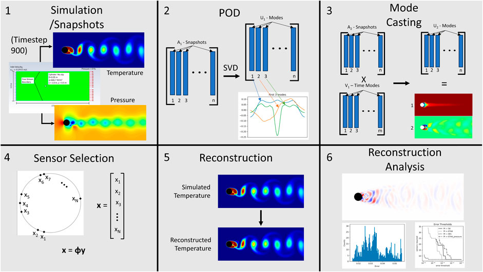
FIGURE 1. Graphical Summary of the method implemented in the paper. It shows: 1) the generation of the snapshots used to train the model from Section 3.1, 2) the method of proper orthogonal decomposition described in Section 2.1, 3) the method of domain extension described in Section 2.3, 4) the method of sensor selection described in Section 3.2 and Section 3.3, 5) the method of reconstruction outlined in Section 2.2 and Section 3.4, and 6) the analysis of the reconstructed data discussed in Section 4.

3 Model implementation

3.1 Numerical methods

ANSYS™ Fluent was used to solve Eqs. 1–3 and model fluid flow over a cylinder. The domain is a rectangle with a heated cylindrical obstruction. The boundary conditions and geometry of the simulation are shown in Figure 2 and Table 1. As noted in Section 2, density, viscosity, and specific heat are held constant at the values specified in Table 1.

FIGURE 2

FIGURE 2. Boundary conditions and mesh used for simulations, further details in Tables 1, 2.

TABLE 1

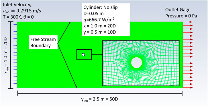
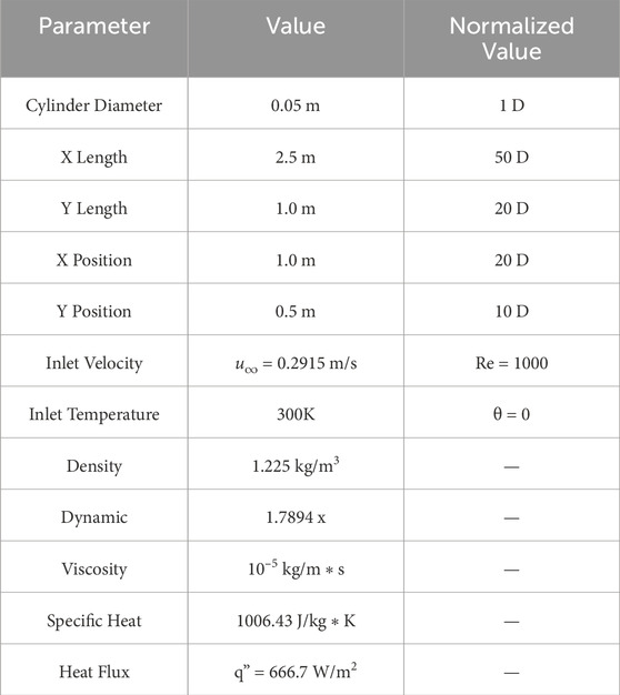
TABLE 1. Details boundary conditions shown in Figure 2.

In their most general mathematical form, the boundary conditions for this work are:

1) Constant flow $\mathbf{u}={[u_{\infty },0]}^T$ at the entrance

2) Constant pressure p = 0 at the exit of the channel

3) Neumann boundary conditions $\frac{\partial \mathbf{u}}{\partial \mathbf{n}}=0$ at the upper and lower boundaries

4) No slip condition, u = 0 on the boundary of the cylinder

5) Constant temperature, θ = 0 at the entrance

6) Constant heat flux, q″ = C on the surface of the cylinder

Lengths are normalized in terms of the diameter of the cylinder D = 0.05 m. A mesh with element size 0.0075 m = 0.15D was used. This was refined to 0.00075 m = 0.015D around the cylinder. This resulted in 48,243 total nodes in the fluid domain and 209 nodes on the perimeter of the cylinder. The mesh is composed of quadratic nodes. The mesh can be seen in Figure 2, though the fine mesh appears solid. The laminar viscous model in Fluent was used, which implies no turbulent flow model approximation.

Initial conditions were obtained by running the simulation until stable flow conditions were obtained, noting the time steps, t required to do this and then running for another 1.5t time steps to ensure truly stable behavior was captured. Constant time steps of 0.0005 s leading to a Courant number of 0.2 were used in the simulation to ensure consistency and high-resolution data in the time domain, though these are not strictly necessary with the method of snapshots. The minimum requirement is that the training data cover the domain of possible states with sufficient temporal resolution. Using a constant time step that was adapted to the period of the Strohaul number is a convenient and easy way to ensure this. Since the SVD execution time depends mostly on the minimum dimension in the A matrix, the inclusion of an excessive number of snapshots ensures adequate domain coverage without significantly impacting runtime. Once stable behavior was achieved, the simulation was continued and data was collected. Pressure and temperature data on the cylinder surface and in the flow volume was sampled every 16 time steps over 32,000 time steps for a total of 2000 snapshots. Increasing the number of snapshots included in the training set beyond 1000 did not noticeably affect results and so 1000 stationary time steps were captured as training data and another 1000 were captured as a test set. The test data in this work is taken directly from the simulation with no accounting for sensor-induced noise. However, in real sensing applications, there is a level of uncertainty in the readings from sensors. This is typically modeled as a layer of Gaussian noise added on top of the sensed signal in controls and sensing applications. Raioli et al. demonstrated that the POD methods used in this paper are still valid when the sensed signal has interference from a Gaussian noise component. They validate a method by which this additional error can be considered and calculated (Raiola et al., 2015). The technique presented in this paper should be coupled with Raioli’s method for implementation in a real-world system.

The simulations were conducted with varying Prandtl numbers to achieve different temperature profiles. To study the effect of varying Prandtl numbers, the thermal conductivity of the fluid in the simulation was varied as detailed in Table 2. A visual representation of this step can be found in Figure 1 pane 1.

TABLE 2

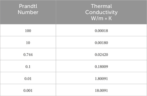
TABLE 2. Thermal conductivity values used to achieve Prandtl numbers.

3.2 Training the model

A trained model consists of two matrices, Φ and Ψ which will be defined subsequently. Given an a priori list of sensors to include, the matrices Ψ and Φ can be calculated independently of one another. However, since the method of selecting sensors used in this work relies on knowledge of Ψ, its calculation is outlined first here.

After the simulations are complete, the data is imported into Python. The data from the cylindrical surface is sorted by angle. This is stored in a matrix, A₁ where columns are snapshots in time and rows are angular position. The data from the rest of the volume is processed by a binning technique for ease of computation and visualization. The domain is divided into 25,000 bins forming a 250 × 100 uniform grid. Then each datapoint is labeled by what bin it falls into. Then all of the datapoints in each bin are averaged and that average is the stored value for the bin. The data for the volume is imported and matrices containing the x and y coordinates are stored for later visualization. The data is then stored in a matrix A₂ where columns are snapshots in time and rows correspond to locations. After the data is stored in matrices A₁ and A₂, SVD is performed on matrix A₁ resulting in matrices U₁, Σ₁, and V₁. This process is repeated for each Prandtl number for which data has been collected.

Now the number of modes to be kept from each profile must be determined. This is typically done by computing the proportion of the energy, p kept by keeping n modes and finding n for which some threshold of energy p_min, e.g., 0.99, 0.999, 0.9999 is kept. Letting the diagonal of Σ = [σ₁, σ₂, … , σ_r], p can be calculated as,

$p=\frac{{\sigma }_1^2+{\sigma }_2^2+\cdots +{\sigma }_n^2}{{\sigma }_1^2+{\sigma }_2^2+\cdots +{\sigma }_r^2}\ge p_{\mathit{min}}(10)$

In this work, the number of modes used is varied as an independent variable and Eq. 10 is used merely to evaluate these selections. Regardless, once the number of modes to be retained for each profile has been determined, $\overline{{\mathbf{U}}_{\mathbf{1}}}$ for each profile can be formed.

Now that the dominant modes have been determined, the corresponding modes of the volume domain can be calculated and stored. For a given profile, the modes of the volume domain are calculated using Eq. 9. The modes are stored in $\overline{{\mathbf{U}}_{\mathbf{2}}}$ and Ψ₂.

We must also construct the matrix Φ which maps from the full domain y with j entries, to the partial, sensed domain x with k entries. To construct Φ from a list of sensors to be kept, create a sparse k × j matrix with a single ‘1′ in each row. Each of these ‘1’s’ should be the only ‘1′ in its column and should correspond to a unique sensor being kept. For example, if y₅, y₃₈, and y₉₇ are the sensed locations, then Φ should have a “1” only in its fifth, 38th, and 97th columns. Figure 1 pane 4 visually describes this process. Now that Ψ and Φ these have been determined, they can be used to create reconstructions from sensed data.

3.3 Sensor selection

The sensor set used throughout this work was determined by examining the locations in the cylinder domain where the modes included in Ψ₁ had absolute maxima and minima. For each temperature profile, the sensor corresponding to the maxima and minima for each mode were listed in order of the mode they came from in a master sensor set. Duplicate sensors were removed. Then, to create shorter sensor sets for analysis, the first n sensors in the list are used, with n being the desired number of sensors for the test. This method has been previously applied to the sensor location problem by Cohen et al. and more recently by Bright et al. and is the generally accepted method for sensor selection in POD based reduced order models (Cohen et al., 2003; Bright et al., 2013). This method is favored in this work because it allows for consistency between the sensor sets and because it is far less computationally intensive than performing the analysis on many random sensor sets that would be required to empirically find better sensor sets.

3.4 Model testing

To test the model, A_1test and A_2test datasets containing snapshots with data at all locations are generated and processed in the same way as the training data. Additionally, an X dataset containing only the data from the sensed locations with each column of X, x_i containing sensed data for a snapshot.

Then for each snapshot, solve Eq. 8 using the methods outlined in Section 2.2. This results in a vector a which contains information about how useful each mode in Ψ₁ is in creating sensor output x_i. a can then be used along with Eq. 9 to solve Eq. 6 and find Y₂ with each column containing a snapshot of the field reconstructed from the sensed data. This step is shown in Figure 1 pane 5.

4 Results

To produce the results presented in this section, the following analysis process was performed for the various datasets generated. As described in Section 3.1, 1000 snapshots of the pressure or temperature field on the cylinder were collected from the simulation. They were formed into a matrix, A and the POD was performed to extract the modes. The method outlined in Section 3.2 was then used to create modes for the pressure or temperature within the volume. A sensor set was then formed using the method outlined in Section 3.3. 23 different models were created, incorporating between 4 and 26 modes. This range of modes was chosen such that a model that retained all but 1e-6% of the energy as calculated by Eq. 10 was included for all cases tested. Each model was then tested with data collected from 21 sensor sets, x_i for 7 ≤ i ≤ 27 where x_i contains the first i sensors in the overall sensor set. Extra sensors were included for some cases. Each model and set of sensors was tested on 1000 test data snapshots using the method presented in Section 3.4 and the statistics described in Section 4.1 were collected. Figure 3 illustrates the testing procedure.

FIGURE 3

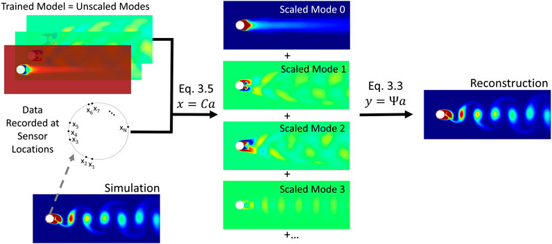
FIGURE 3. Sensed data is used to find scaling values for modes which are then summed to generate a reconstructed field.

4.1 Error evaluation

Two error metrics are considered to provide a basis for quantitative comparison between reconstructions and snapshots. Before implementing either error metric, the data is normalized as $\theta =\frac{x-x_{\mathit{min}}}{x_{\mathit{max}}-x_{\mathit{min}}}$ where x is the quantity being analyzed. x_max and x_min are evaluated over all test snapshots so that θ is a normalized scale with range 0–1 across the whole domain being studied.

The L₂ error norm,

$\epsilon =\Vert {\theta }^{\mathit{ref}}-{\theta }^{\mathit{calc}}{\Vert }_2/\Vert {\theta }^{\mathit{ref}}{\Vert }_2(11)$

where θ^ref is the snapshot of the field produced by the simulation discussed in Section 3.1 and θ^calc is the reconstructed snapshot provides a measure of how similar the reconstruction is to the reference overall. Both θ′s are vectors with dimension equal to the number of points in the field, in this case 25,000. The L₂ norm is the length of a vector in that 25,000 dimensional space. ɛ is therefore the distance between the reference value and calculated value in that space, divided by length of the reference value and gives a sense of the overall similarity between snapshots (Fukami et al., 2021; Zhong et al., 2023).

The absolute error at a grid point (i,j), $|e_{i,j}|\equiv |{\theta }_{i,j}^{\mathit{ref}}-{\theta }_{i,j}^{\mathit{calc}}|$. The maximum absolute error (MAE) is the maximum |e_i,j| over all grid points in a given snapshot. The MAE of a snapshot indicates how well the reconstruction matches the reference value at its worst grid point. This error metric gives a bound on the accuracy of the reconstructed values at each point whereas the L₂ error norm from Eq. 11 only gives an overall sense of similarity and can thus smooth over large inaccuracies at individual points (Jiang et al., 2017).

The test data set for each temperature profile contains 1000 snapshots. 1000 values for ɛ and MAE are thus calculated for each sensor and mode configuration tested. The maximum values of ɛ and MAE over these 1000 snapshots are reported as ɛ_max and MAE_max. Likewise the mean values over 1000 snapshots are reported as ɛ_mean and MAE_mean. These composite error metrics provide information about the reconstruction success across all snapshots.

4.2 Reconstruction of pressure fields from sensed pressure data

For a given number of modes, ɛ_mean decreases as sensors are added up to a cutoff point, after which the addition of sensors made little difference. Figure 4 shows this behavior for models containing select numbers of modes with black circles roughly indicating the point of diminishing return. For relatively low numbers of included sensors, the models containing fewer modes yield the lowest error as they reach the point of diminishing return quickly and display asymptotic behavior over most of the range of sensors. ɛ_mean for a given number of sensors tends to be higher when more modes are included in the model if those models do not include sufficient sensors to their asymptotic ɛ_mean. ɛ_mean generally decreases with the number of sensors included before reaching its asymptotic value. For increasing numbers of modes included in a model, the number of sensors required to reach asymptotic ɛ_mean increases while that asymptotic value of ɛ_mean decreases, indicating an improvement in flow field reconstruction.

FIGURE 4

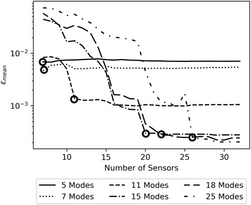
FIGURE 4. Variation of ɛ_mean with number of sensors for Pressure data. Black circles indicating the beginning of asymptotic behavior.

The asymptotic behavior indicates that, for a desired level of error in the reconstructions from a sparsely sensed system, there is a minimum number of modes and a corresponding minimum number of sensors required to produce reconstructions with that level of error. Figure 5A displays the relationship between the number of modes included in the model and the asymptotic error resulting from the model. While all measures of error decrease with increasing numbers of modes, ɛ_mean and MAE_mean are noticeably smoother and monotonically decrease. The relation between the number of sensors included in the model and the resulting error, shown in Figure 5C displays similar behavior but is discontinuous at points, with sudden decreases in achievable error. The error decreases relatively little as less necessary sensors are added but then falls sharply when a particularly useful sensor is added which allows the model to leverage more modes. When considered together Figures 4, 5A characterize the relation between sensors, modes, and reconstruction accuracy for the model when trained on pressure data.

FIGURE 5

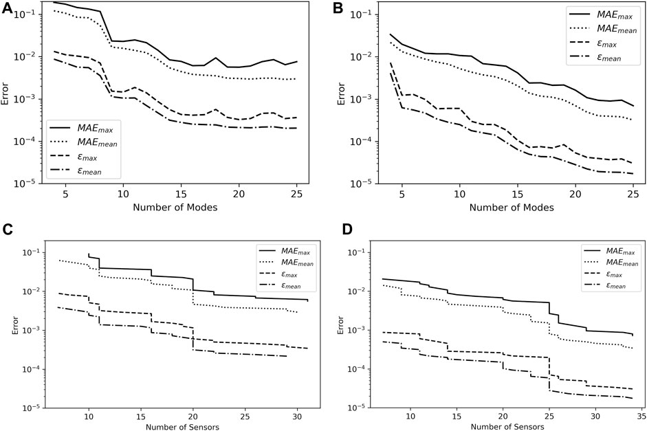
FIGURE 5. Asymptotic and sensor error comparison for pressure and temperature. (A) Asymptotic error values for pressure. (B) Asymptotic error values for temperature data, Pr = 0.744. (C) Best case error for a given number of sensors for pressure data. (D) Best case error for a given number of sensors for temperature data, Pr = 0.744.

4.3 Reconstruction of temperature fields from sensed temperature data for Pr = 0.744

With the model and method of analysis now developed for the pressure case, the procedure of Section 4.2 is applied using training and test sets composed of temperature data for Pr = 0.744, which corresponds to air. Figures 5B, D show the relationship between the number of modes and sensors included in the model and the resultant error analogous to Figures 5A, C. The relation between the number of modes included in the model to error for the temperature data is similar in shape to that for the pressure data. All measures of error, especially the mean measures, decrease with the number of modes included in the model. However, the temperature data yields far lower MAE and ɛ than the pressure data. MAE_mean varies from 0.022 to 0.00032 for the temperature data and 0.121–0.0030 for the pressure data. The discrepancy is similar for ɛ_mean, which varies from 0.0041 to 0.0000173 for the temperature data and 0.0087–0.00021 for the pressure data.

These metrics suggest that the temperature field can be reconstructed with about 1/10th the error of the pressure field. In the wake region, the low points in pressure correspond to vortices shed from the cylinder. These vortices are coherent and persist in the flow long after they leave the simulated region. Error values are relatively high when the algorithm predicts the locations or intensities of one or many of these vortices poorly. Since relatively large perturbations are present in the pressure field from the edge of the cylinder to the edge of the simulation, there are many points at which the reconstruction may depart from the test data significantly, thus producing relatively high error values. In the temperature field, hot spots form from contact with the cylinder as the vortices are formed. The hot spots cool quickly as thermal energy diffuses into the surrounding cooler fluid. By the time the vortices reach the simulation boundary, much of the thermal energy has diffused into the surrounding fluid. This means that, compared to the pressure field which has persistent low-pressure peaks all the way to the edge of the simulation, the temperature field contains a few similar high-temperature eddies in the immediate wake of the cylinder which become lower-temperature eddies as they move away from the cylinder. When these lower-temperature eddies are predicted poorly, they do not result in as large of an impact on the error as a poorly predicted high-temperature eddy would. Thus ture fluctuations compared to that of pressure fluctuations.

4.4 Reconstruction of temperature fields from sensed temperature data for varying Prandtl number

To test the hypothesis of thermal energy diffusion leading to better reconstructions for temperature than for pressure, flows of varying Prandtl number are considered. At a high Prandtl number, ν ≫ α, meaning the conduction of heat away from the vortices is held to a minimum. The high Prandtl number mostly inhibits the effect of thermal diffusion that is postulated to disrupt comparison between pressure and temperature reconstructions.

To provide a deeper understanding of the effects of Prandtl number on temperature field reconstruction from sparsely sensed data, flows with Pr = 50, 10, 0.744, 0.1, 0.01, and 0.001 are considered. Because constant material properties were used in the simulation, temperature fluctuations have no effect on momentum transport between the simulations, and thus the pressure field from Section 4.2 is the pressure field for all cases.

Figure 6 shows the MAE_mean for the different systems studied and Figure 7 shows the ɛ_mean. Both the MAE_mean and ɛ_mean are very similar between the pressure and the temperature for flows with Pr = 50 and 10, especially when 10 or more modes are included in the model. The similar reconstruction success between temperature in high Prandtl number flows and pressure confirms the hypothesis from Section 4.3.

FIGURE 6

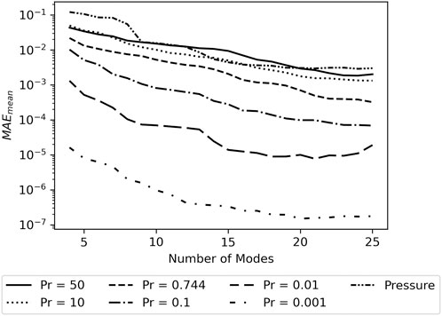
FIGURE 6. Asymptotic MAE_mean for different Prandtl numbers.

FIGURE 7

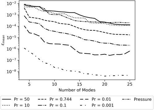
FIGURE 7. Asymptotic ɛ_mean for different Prandtl numbers.

Figure 8 gives a summary of the MAE_max for temperature reconstruction in terms of number of sensors included in the model and the Prandtl number of the fluid. It confirms the trend of decreasing error as the number of sensors increases and the Prandtl number of the fluid decreases. Reporting the value of MAE_max in terms of the number of sensors leaves the result somewhat sensitive to the effect of sub-optimal sensor sets. Results incorporating a better sensor selection method would yield lower error and would likely create a more uniform gradient. However, the data as reported is more useful as a baseline for the reader that wishes to apply this technique with their own experimental or simulated data. MAE_max indicates the severity of a worst case scenario prediction allowing the user to calibrate their application of this technique to their needs.

FIGURE 8

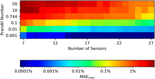
FIGURE 8. Shows the MAE_max over a range of Prandtl numbers and numbers of sensors.

5 Conclusion

In this paper, the POD inferencing technique was successfully applied to temperature and pressure fields, and a pseudoinverse solving technique was implemented to extend this method from classification to a focus on reconstruction of the field variables. The refined algorithm was tested on pressure and temperature data from flows with Prandtl numbers varying between 0.001 and 50. POD inferencing models with 4 and 26 modes were trained and their performance was tested over sensor sets containing between 7 and 27 sensors. The MAE_mean and ɛ_mean error metrics were considered and applied to evaluate the performance of the algorithm for varying Prandtl numbers, numbers of modes, and numbers of sensors. All error metrics were found to vary heavily as the Prandtl number was changed with low Prandtl numbers resulting in the lowest error. This implies that fewer sensors are required for accurate temperature field reconstruction for low Prandtl number fluids. Models with more modes generally outperformed those with fewer modes as implied by measures of mode energy content. For a given dataset and number of modes, an increase in the number of sensors was found to improve prediction accuracy up to a point, after which the additional sensors had little impact. This is valuable information for design, as it indicates that in applications where a given reconstruction error is desired, the number of modes required to yield that error can first be determined. Then the number of sensors, now limited by the number of modes, and their locations can be determined. The reconstruction error was shown to be comparable between pressure and temperature in high Prandtl number fluids. In moderate Prandtl number fluids such as air, and low Prandtl number fluids, thermal dissipation smooths temperature gradients, leading to lower error in temperature reconstruction relative to pressure. Future work will study the application of this method to turbulent flow data and attempt to generalize the relation between Prandtl number, reconstruction error, and mode energy content.

Data availability statement

The raw data supporting the conclusion of this article will be made available by the authors, without undue reservation.

Author contributions

JM: Conceptualization, Data curation, Investigation, Methodology, Visualization, Writing–original draft, Writing–review and editing. HB: Conceptualization, Funding acquisition, Project administration, Resources, Software, Supervision, Writing–review and editing.

Funding

The author(s) declare financial support was received for the research, authorship, and/or publication of this article. The work presented was supported by the U.S. Department of Energy, Nuclear Energy University Program, under Award Number DE-NE0009153 and US Nuclear Regulatory Commission under grant no. 31310021M0044. Funding for publishing was provided by Purdue University Libraries Open Access Publishing Fund.

Conflict of interest

The authors declare that the research was conducted in the absence of any commercial or financial relationships that could be construed as a potential conflict of interest.

The author(s) declared that they were an editorial board member of Frontiers, at the time of submission. This had no impact on the peer review process and the final decision.

Publisher’s note

All claims expressed in this article are solely those of the authors and do not necessarily represent those of their affiliated organizations, or those of the publisher, the editors and the reviewers. Any product that may be evaluated in this article, or claim that may be made by its manufacturer, is not guaranteed or endorsed by the publisher.

References

Agrawal, A., Verschueren, R., Diamond, S., and Boyd, S. (2018). A rewriting system for convex optimization problems. J. Control Decis. 5, 42–60. doi:10.1080/23307706.2017.1397554

CrossRef Full Text | Google Scholar

Ahmed, Z., Jordan, C., Jain, P., Robb, K., Bindra, H., and Eckels, S. J. (2022). Experimental investigation on the coolability of nuclear reactor debris beds using seawater. Int. J. Heat Mass Transf. 184, 122347. doi:10.1016/j.ijheatmasstransfer.2021.122347

CrossRef Full Text | Google Scholar

Batchelor, G., Howells, I., and Townsend, A. (1959). Small-scale variation of convected quantities like temperature in turbulent fluid part 2. the case of large conductivity. J. Fluid Mech. 5, 134–139. doi:10.1017/s0022112059000106

CrossRef Full Text | Google Scholar

Batchelor, G. K. (1959). Small-scale variation of convected quantities like temperature in turbulent fluid part 1. general discussion and the case of small conductivity. J. fluid Mech. 5, 113–133. doi:10.1017/s002211205900009x

CrossRef Full Text | Google Scholar

Bright, I., Lin, G., and Kutz, J. N. (2013). Compressive sensing based machine learning strategy for characterizing the flow around a cylinder with limited pressure measurements. Phys. Fluids 25, 127102. doi:10.1063/1.4836815

CrossRef Full Text | Google Scholar

Buchan, A., Pain, C., Fang, F., and Navon, I. (2013). A pod reduced-order model for eigenvalue problems with application to reactor physics. Int. J. Numer. Methods Eng. 95, 1011–1032. doi:10.1002/nme.4533

CrossRef Full Text | Google Scholar

Candes, E. J., Romberg, J. K., and Tao, T. (2006). Stable signal recovery from incomplete and inaccurate measurements. Commun. Pure Appl. Math. A J. Issued by Courant Inst. Math. Sci. 59, 1207–1223. doi:10.1002/cpa.20124

CrossRef Full Text | Google Scholar

Chen, M., Liu, S., Sun, S., Liu, Z., and Zhao, Y. (2020). Rapid reconstruction of simulated and experimental temperature fields based on proper orthogonal decomposition. Appl. Sci. 10, 3729. doi:10.3390/app10113729

CrossRef Full Text | Google Scholar

Cohen, K., Siegel, S., and McLaughlin, T. (2003). “Sensor placement based on proper orthogonal decomposition modeling of a cylinder wake,” in 33rd AIAA Fluid Dynamics Conference and Exhibit, China, February 2022 (IEEE), 4259.

CrossRef Full Text | Google Scholar

Diamond, S., and Boyd, S. (2016). CVXPY: a Python-embedded modeling language for convex optimization. J. Mach. Learn. Res. 17, 83–85.

PubMed Abstract | Google Scholar

Eckart, C., and Young, G. (1936). The approximation of one matrix by another of lower rank. Psychometrika 1, 211–218. doi:10.1007/bf02288367

CrossRef Full Text | Google Scholar

Epps, B. P., and Krivitzky, E. M. (2019). Singular value decomposition of noisy data: mode corruption. Exp. Fluids 60, 121–130. doi:10.1007/s00348-019-2761-y

CrossRef Full Text | Google Scholar

Fukami, K., Maulik, R., Ramachandra, N., Fukagata, K., and Taira, K. (2021). Global field reconstruction from sparse sensors with voronoi tessellation-assisted deep learning. Nat. Mach. Intell. 3, 945–951. doi:10.1038/s42256-021-00402-2

CrossRef Full Text | Google Scholar

Gould, D. W., Bindra, H., and Das, S. (2017). Thermal response construction in randomly packed solids with graph theoretic support vector regression. Int. J. Heat Mass Transf. 115, 421–429. doi:10.1016/j.ijheatmasstransfer.2017.07.063

CrossRef Full Text | Google Scholar

Jiang, C., Soh, Y. C., and Li, H. (2017). Two-stage indoor physical field reconstruction from sparse sensor observations. Energy Build. 151, 548–563. doi:10.1016/j.enbuild.2017.07.024

CrossRef Full Text | Google Scholar

Jiang, G., Kang, M., Cai, Z., Wang, H., Liu, Y., and Wang, W. (2022). Online reconstruction of 3d temperature field fused with pod-based reduced order approach and sparse sensor data. Int. J. Therm. Sci. 175, 107489. doi:10.1016/j.ijthermalsci.2022.107489

CrossRef Full Text | Google Scholar

Liu, Y., Liu, C.-H., Brasseur, G. P., and Chao, C. Y. (2023). Proper orthogonal decomposition of large-eddy simulation data over real urban morphology. Sustain. Cities Soc. 89, 104324. doi:10.1016/j.scs.2022.104324

CrossRef Full Text | Google Scholar

Lu, K., Jin, Y., Chen, Y., Yang, Y., Hou, L., Zhang, Z., et al. (2019). Review for order reduction based on proper orthogonal decomposition and outlooks of applications in mechanical systems. Mech. Syst. Signal Process. 123, 264–297. doi:10.1016/j.ymssp.2019.01.018

CrossRef Full Text | Google Scholar

Lumley, J. (1981). “Coherent structures in turbulence,” in Transition and turbulence. Editor R. E. MEYER (Cambridge: Academic Press), 215–242.

CrossRef Full Text | Google Scholar

Luo, Z., and Chen, G. (2018). Proper orthogonal decomposition methods for partial differential equations. Cambridge: Academic Press.

Google Scholar

Panton, R. L. (2013). Incompressible flow. USA: John Wiley amp; Sons.

Google Scholar

Penrose, R. (1956). On best approximate solutions of linear matrix equations. In Mathematical Proceedings of the Cambridge Philosophical Society, 52. Cambridge: Cambridge University Press, 17–19.

CrossRef Full Text | Google Scholar

Raiola, M., Discetti, S., and Ianiro, A. (2015). On piv random error minimization with optimal pod-based low-order reconstruction. Exp. fluids 56, 75–15. doi:10.1007/s00348-015-1940-8

CrossRef Full Text | Google Scholar

Sirovich, L. (1987). Turbulence and the dynamics of coherent structures. i. coherent structures. Q. Appl. Math. 45, 561–571. doi:10.1090/qam/910462

CrossRef Full Text | Google Scholar

Sirovich, L., and Park, H. (1990). Turbulent thermal convection in a finite domain: Part i. theory. Phys. Fluids A Fluid Dyn. 2, 1649–1658. doi:10.1063/1.857572

CrossRef Full Text | Google Scholar

Ward, B., Clark, J., and Bindra, H. (2019). Thermal stratification in liquid metal pools under influence of penetrating colder jets. Exp. Therm. Fluid Sci. 103, 118–125. doi:10.1016/j.expthermflusci.2018.12.030

CrossRef Full Text | Google Scholar

Wolfram, S. (2023). Computational foundations for the second law of thermodynamics. USA: Stephen Wolfram Writings RSS.

Google Scholar

Zhong, Y., Fukami, K., An, B., and Taira, K. (2023). Sparse sensor reconstruction of vortex-impinged airfoil wake with machine learning. Theor. Comput. Fluid Dyn. 37, 269–287. doi:10.1007/s00162-023-00657-y

CrossRef Full Text | Google Scholar