A framework for the practical development of condition monitoring systems with application to the roller compactor

1 Motivation

Abnormal conditions in pharmaceutical manufacturing need to be corrected before they can degenerate further and start compromising product quality, equipment health, and operator safety. Without timely intervention of these faulty conditions, operators could be forced to perform costly product diversions and process shutdowns; and if they happen frequently enough, they could negatively offset any potential benefit of shifting pharmaceutical manufacturing from batch to continuous mode. Lee et al. (2015); Schenkendorf, (2016); Ganesh et al. (2020) Maintaining steady-state operation for continuous systems thus requires not only effective process control but also real-time monitoring of the system condition; faults need to be detected and diagnosed promptly so that appropriate maintenance activities can be promptly performed Venkatasubramanian et al. (2003b); Ganesh et al. (2020).

Implementing this condition-based maintenance strategy requires an effective condition monitoring system, which is challenging to develop because of the evolutionary nature of drug production process development. Drug manufacturing process systems often utilize equipment with varying levels of technology, different levels of control, Su et al. (2019) and with already existing but incomplete fault detection and diagnostic capabilities. Furthermore, development of condition monitoring systems traditionally employs data-driven methods that require large amounts of data while largely ignoring expert knowledge of the process; this is problematic for pharmaceutical processes where initial process data is expensive to acquire.

A further challenge to developing CM systems is the lack of a complete fault library during process development. This has at least two major consequences: existing CM systems must be able to manage novel faults as they are discovered, Venkatasubramanian et al. (2003b) and existing CM systems must be retrained to be able to classify these novel faults after discovery. Furthermore, there is no way to evaluate the observability of a process condition; given several existing CM systems monitoring a process, are they sufficient to observe the process condition, or do additional CM systems need to be developed, and on what section of the process?

A practical solution is needed to navigate through these complexities and this paper reports on a proposed solution that centers on a four-stage framework. Using a pharmaceutical roller compactor unit as an example, the capabilities and advantages of the framework are discussed including the ability to manage novel faults.

2 Primer on condition monitoring

Condition monitoring has been a subject of research for at least 6 decades now. It has traditionally been applied to monitoring the condition of major equipment such as jet engines, power stations, and railway equipment. The underlying motivation for these systems is safety, particularly of the equipment and the workers interacting directly with the equipment, and this is true across the chemical process industries, where condition monitoring is applied to unit operations equipment to improve reliability and safety.

In chemical processing, safety concerns are often treated separately from product quality, even though the former can have ramifications on the latter. This might be because of the differences in addressing them. Occurrence of safety incidents and accidents typically require a series of events to align (as per the Swiss cheese model) and they generally occur infrequently; thus, monitoring is sufficient. Product quality deviations are likely to happen more frequently, often necessitating active process control to mitigate this issue.

As a result, condition monitoring systems in manufacturing processes tend to be comprised of disparate systems that work independently of each other. With this approach, it is unclear if these independent systems are providing complete visibility of the process condition. Furthermore, their autonomy prevents the capitalization of potential causal dependencies that one system might have on the other.

2.1 Safety in condition monitoring

The proposed framework addresses the limitations of having autonomous condition monitoring systems, particularly between systems that address safety and product quality. The first step in achieving this is to subsume product quality as one of the facets of safety. This is possible for a pharmaceutical manufacturing application because a poor-quality drug could have a negative impact on the treatment and health of the patient consuming the drug. Furthermore, product quality monitoring most likely sources its data from the same sensors and machine data; so, it makes sense to treat them under a unified framework. Hence, throughout the remaining discussions in this paper, we will refer to safety as either operator safety, equipment safety, or consumer/patient safety.

However, although it is convenient to view these facets of safety as separate, there is a directed relationship between them. Failures that affect operator and equipment safety tend to affect product quality because safety systems address these failures through mandatory shutdowns, thereby stopping the manufacturing process and its associated control systems. However, this dependency does not necessarily flow in the other direction, as product quality issues tend to remain a product quality concern and do not necessarily translate into an operator or equipment safety problem. It will be apparent in Section 4.1 that this observation is important, since it influences the methodology behind the Representation stage, which is the first stage of the proposed framework.

2.2 Anatomy of a failure

A failure is a condition where safety (operator, equipment, or product quality) is compromised, and an emergency shut down is necessary to prevent further damage and possibly loss of life. The goal of condition monitoring is to prevent failures by detecting them at their onset, which is when they are still considered a fault. A fault can henceforth be considered as the root cause of a failure, or one of the root causes if the failure is a result of multiple faults Venkatasubramanian, (2011). The root cause does not necessarily compromise safety, at least not right away. However, it needs to be detected and corrected before it leads to an unsafe situation.

This implies that a fault is not a failure, although the terms are often used synonymously. This is an important distinction to point out because a system can perform in a state of fault, or even with multiple simultaneous fault events, without any undesired consequences to safety. It is when a failure occurs, as a result of one or more uncorrected faults, that safety is compromised with consequences for the operators, equipment, or product quality.

Figure 1 shows an example of condition monitoring where API concentration is measured at the outlet of a powder blender to monitor product quality. A fault was induced at the 20-minute mark, which means that something abnormal happened. In this case, the feeder control system starts to malfunction. At this point, a fault is present, but everything still looks normal from the perspective of the dataset; the fault is currently undetectable.

Figure 1

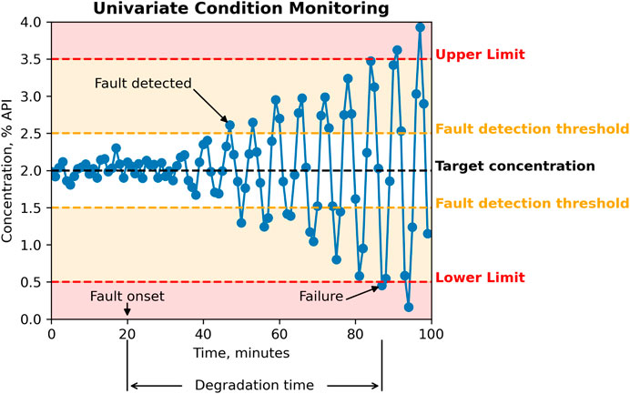
Figure 1. Univariate condition monitoring.

Faults at their onset are not necessarily detectable. For the API concentration example, it could be that the extent of malfunction is not yet significant at the beginning, or the blender control system is somehow mitigating the effects of a faulty API feeder. As the fault worsens, the sensor signals start deviating away from “normal” conditions and starts to match its fault signature, eventually reaching detectability.

In practice, fault detection and diagnosis entail real-time monitoring of one or more variables. The traditional way is to use a univariate approach, where the fault would be detected if one or more variables exceed the fault detection threshold. This can become impractical as the process scale increases with more sensors installed and thus more advanced approaches such as Principal Components Analysis (PCA) become useful. With such techniques, the sensor signals are combined and projected onto principal components, and a few outlier detection statistics can then be monitored instead of individually monitoring a large number of highly correlated variables.

Although the concept of a fault detection threshold could become moot by using such techniques, it is important to understand the distinction between fault onset and fault detectability, what affects fault detectability, and how earlier detection can allow more time for implementing the best possible response to the fault.

2.3 Symptoms and sensors

Reducing the time from fault onset to detection is one of the primary considerations in designing a condition monitoring system. This can be achieved by using more sensitive sensors, generating more information by adding more sensors, and/or by signal processing; all of which effectively lower the detection threshold. The sooner the fault is detected after onset, the longer the time available between fault detection and failure and thus the time available for implementing the critical activity of responding appropriately to the fault.

These measures allude to the relationship between a fault and its symptoms. Symptoms are the data signatures of a fault, which are a collection of process variable values, both measured and unmeasured, that are characteristic of that fault. It can be assumed that the symptoms start appearing immediately at the fault onset, but not all symptoms are manifested until after the fault has progressed to failure to a certain degree. Often, the more immediately manifesting symptoms are currently unmeasured, if not unmeasurable by a process system. It can then be surmised that a fault can be detected earlier by targeting the measurement of symptoms that would happen immediately at fault onset. This could be an additional objective and significance in the deployment of PAT sensors for monitoring, control, and real-time release.

Although the ability of a condition monitoring system to detect a fault depends on the ability of any of the process sensors to capture the symptoms, it does not require that all the symptoms are measured; at least just one needs to be captured. However, it is possible that multiple faults share the same symptom, so discriminating between these faults depends on capturing other symptoms that are unique to each fault. It is also possible that some symptoms persist throughout the occurrence of fault, while some do not. If a condition monitoring system is working with symptoms that do not persist, then training a system to detect that fault could be challenging.

It is thus important to know beforehand the nature of the symptoms that are measured by the system, since developing a condition monitoring system on symptoms that are not persistent and unique would definitely lead to condition classification problems. It would be more effective to pursue efforts to capture the proper symptoms before attempting to train a classification model to detect and diagnose these faults.

2.4 Condition monitoring and active control

Because condition monitoring systems are intended for the implementation of condition-based maintenance, they can only deal with faults that take a relatively long time to degrade into a failure. A fault with a degradation time in the order of hours to days would be applicable as this allows ample time for a response via maintenance by a human operator.

At the other end of the spectrum are faults with degradation times in the order of seconds, or minutes. These cannot be managed via condition-based maintenance. Rather, active process control or a process redesign is required, especially if the magnitude of failure impact is expected to be severe.

Initially, all known faults in a fault library would have long degradation times. As more knowledge is generated throughout the life of a process system, newly discovered faults that have very short degradation times should prompt a process redesign. If this is not possible, an active process control could be installed to mitigate the degradation. Doing this transforms the fault into another type of fault, namely that of the active control system malfunctioning—which ought to take a long time as a result of a proper design. It can then be argued that such active control systems effectively transform faults with short degradation time into faults that occur less frequently and degrade slowly, thereby allowing ample time for detection and intervention.

A safe process system could be ultimately characterized as a system that has no known faults with short degradation times, and an effective fault management system would be one that can detect unknown faults and classify them according to their degradation times. As these faults are discovered, active process control systems ought to be installed to manage them, and the faults with long degradation times would then be added to the fault library, where future occurrences of the fault could be automatically detected by a condition monitoring system and then addressed via maintenance activities.

2.5 Special faults

The degradation time of fault from onset to failure can take a long time, in the order of days or weeks. Sometimes, it could be economical to allow the fault to linger and to delay maintenance activities until a reasonable time to failure remains. This practice is called predictive maintenance, and it is a subset of the condition-based maintenance paradigm. It is beyond the scope of the proposed framework, but it is important to mention the dangers of allowing a fault to linger until it economically makes sense to take action.

Even if a fault might take a very long time to failure, it should still be detected and addressed promptly. This is especially true if the degradation time decreases rapidly in combination with other faults. This is consistent with the Swiss cheese model in process safety where the deficiencies in each layer of protection line up to allow a safety incident to occur. The lining up of each layer protection is similar to the simultaneous occurrence of multiple faults that by themselves could take a very long time to occur, but when occurring concurrently could lead to rapid progression into a failure.

Another type of fault that rarely goes to failure, but needs to be detected, are self-correcting faults. These are faults that do not always degrade into failure but return to normal condition even without intervention. An example of this would be short-term temperature and humidity disturbances that could potentially affect powder properties. If undetected, process managers would be unaware of near misses on the product quality. Although nothing happened, future occurrences of the fault might reach failure before self-correcting. It is best to develop a condition monitoring system that can detect these faults so they can be investigated. Learning from these faults could lead to useful adjustments on the process design and/or operation to prevent them from happening again.

2.6 The condition library

Condition monitoring is essentially the practice of fault detection and diagnosis (FDD), and practitioners usually refer to them synonymously. However, there are key differences between them that need to be discussed in order to avoid confusion in the ensuing sections.

Firstly, FDD practitioners usually approach fault detection and diagnosis separately. For example, fault detection could be performed by monitoring outlier statistics of PCA and comparing them against a pre-determined threshold, similar to the fault detection threshold discussed in Figure 1. Once a fault is detected, diagnosis would then be performed in a different manner—e.g., analyzing patterns in the contributions plot to classify which fault occurred.

Under the aforementioned approach, the PCA contributions plots can be considered the fault signatures, and these would be stored and labelled in a fault library. Upon detection of a fault, the human operator could then extract the contributions plot of the current data and compare it with the plots from the fault library. If one of the plots matches, a diagnosis could be made.

This is a typical approach to FDD when pattern recognition during fault diagnosis is made by a human, albeit fault detection could still be automated in this manner. However, when FDD is fully automated, where pattern recognition is performed by an Artificial Intelligence agent, a fault library that contains the data signatures (e.g., contribution plots) is no longer relevant. This information is already embedded in the machine learning model, which takes in the pre-treated process data, and reports the predicted fault.

In automated cases, the concept of a fault library becomes relevant during model development for fault diagnosis, not during fault diagnosis. Because model development requires discrimination of machine learning models and data pre-treatment techniques, the process data contained in the fault library should no longer be limited to certain features such as contribution plots. It should contain as much of the data possible, and in their rawest form as possible; the fault library effectively becomes the training dataset for machine learning model development. This facilitates the retraining of the model as better machine learning models and data pre-treatment methods are discovered, and as new faults are experienced and identified.

With the use of classification machine learning models, fault detection and diagnosis can be performed as a single operation. The model takes the pre-processed process data as input, and typically reports probabilities of each possible condition, including the normal condition. Hence, it would make sense to refer to the training data for these models as a condition library instead of fault library, since it now includes data during normal conditions.

Even though detection and diagnosis do not have to be separate operations with the use of traditional classification models, it could still be implemented as a sequential process for computational efficiency. Especially if computational resources are limited, it might be a good idea to implement two models hierarchically: one for classifying between normal condition and faulty conditions, and another one for classifying among the faulty conditions. For the first model, all the known faults could be lumped as one condition, and the classification job would be reduced to a “one-vs-all” classification approach where the model would either predict if the process is normal or faulty. Running the second model would only be necessary if the prediction of the first one was a faulty condition; the second model would then classify the condition among all the fault types. This hierarchical approach can be implemented explicitly, or implicitly as one of the standard implementations of machine learning models. Regardless, the condition library remains the same, a dataset for training classification models.

2.7 Development of sensors and condition monitoring systems

The condition library rarely has the complete set of possible faults for a process, especially in the initial stages of process development. One of the reasons for this is the lack of appropriate sensors that can monitor the pertinent data signatures for the fault. It could also be that a fault shares data signatures with another fault, and the process does not have the differentiating sensors that can discriminate between the two. Hence, these similar faults could be initially classified as one. Thus, the ability of a condition monitoring system to properly detect faults is not just about the classification models being deployed, or the quality and quantity of the training data, but also of the availability of data sources that can provide the right features for classification.

It is often the case that the appropriate sensors could be installed in the later stages of process development and new faults would be discovered along the way and added to the fault library. It is thus very important that the condition monitoring systems should have the flexibility to handle a dynamic fault library and allow frequent retraining of the machine learning models that need to be able to classify the newly discovered faults. This flexibility is a key feature of this proposed condition monitoring framework.

3 Application case study: roller compactor

For purposes of illustrating the proposed framework we consider a simple case study centered on the WP-120 Roller Compactor by Alexanderwerk (Becker-Hardt, 2018). Although housed as a single machine, it is comprised of multiple unit operations with aggregate control systems. Material transformations also occur multiple times as the powder blend turns into ribbon and then into granules. This is illustrated in Figure 2, which shows the material transformations and the unit operations involved.

Figure 2

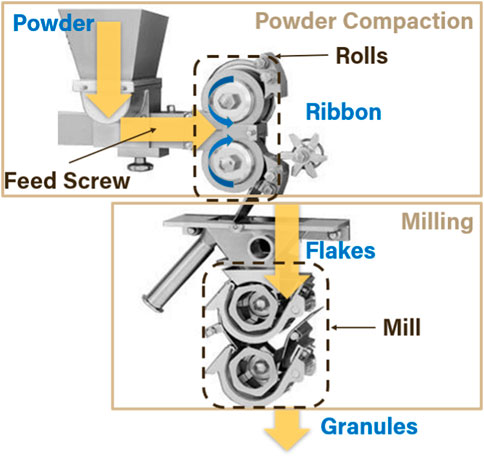
Figure 2. Schematic of the WP-120 roller compactor.

3.1 Roller compactor components and control systems

The RC schematic in Figure 2 shows two main sections: the powder compaction and the milling section. The powder compaction section comprises a feed screw that pushes the powder from the hopper into two counter-rotating rolls, forming the ribbon. The lower roll is at a fixed position while the upper roll is movable. A hydraulic pressure unit pushes this upper roll at a set pressure towards the lower roll, and this pressure can be controlled from the control panel of the RC; roll pressure is one of the parameters affecting the density of the ribbon and is a key variable for condition monitoring of the RC.

Under a given roll pressure, the upper roll may also be set at a nominal position to set the roll gap (i.e., the gap between the upper and lower rolls), which is an important parameter that affects the ribbon width. This is achieved by activating the gap controller, which maintains the roll gap under any roll pressure settings by manipulating the speed of the feed screw. If the roll gap is increased, then more material is required to maintain the roll pressure, and the gap controller increases the feed screw speed accordingly. Conversely, the gap controller will decrease the feed screw speed if the roll gap is decreased.

The gap controller will also respond to the changes in the roll pressure settings. Increasing the pressure will prompt the gap controller to increase the feed screw speed, since a higher pressure will squeeze the ribbon more tightly, effectively lowering the roll gap. Conversely, the controller will decrease the feed screw speed in response to a lower roll pressure setting.

In the milling section of the RC, the ribbon is broken into flakes, and which are then milled into granules by two screen mills, each of which involves a rotating “hammer” that breaks and grinds the flakes until they become small enough to pass through the screen. The distance between the hammer and the screen is one of the controllable parameters of the milling operation, as well as the rotation speed of the hammers. The rotation speed of both mills can only have one setting, but the hammer-screen distances could be different for the upper and lower mills. The upper mill is the first screen mill through which the flakes pass and usually has a larger screen size than the lower mill. The screen size of the lower mill mainly determines the range of the particle size distribution of the product granules, but it is a combination of the screen sizes of the upper and lower mills, the distance between the rotary hammers and the screens, and the rotation speeds of the hammer that would determine the final size and shape distributions of the product granules Akkisetty et al. (2010); Kazemi et al. (2016); Sun et al. (2018).

3.2 Roller compactor condition monitoring systems

Similar to larger scale manufacturing systems, the RC has a built-in CM system that is focused on equipment and operator safety, but not necessarily on the process condition. Hence, such CM components are useful, but incomplete, and would require additional CM systems that could handle faults related to the process condition. This is a common experience in larger systems, and it begs the question of how to handle them.

One alternative would be to ignore these existing systems and create an entirely new CM system that covers all unit operations. In an ideal world where data is free, it might be possible to develop a machine learning model that can achieve this. However, data is expensive in pharmaceutical manufacturing, especially during process development. Moreover, maintaining this model would be challenging as the process potentially evolves to incorporate additional unit operations and as new types of conditions (or faults) are discovered. A more sensible option would be to determine which parts of the process the existing built-in CM systems are monitoring, identify the blind spots and develop CM systems for the blind spots, and then to make these systems work collectively. However, this alternative comes with challenges.

Different CM systems tend to focus on either operator and equipment safety or product quality. It would be tempting to drop one for the other, but this is not recommended since operator and equipment failures do have a direct impact on product quality. These CM systems also tend to work at different timescales, where systems focused on equipment and operator condition tend to operate within seconds or minutes, and CM systems focused on product quality tend to operate within minutes or hours.

The proposed framework for developing CM systems for a pharmaceutical manufacturing process can address these issues, allowing for a practical development of CM systems where existing but incomplete systems can be utilized and integrated into newer ones to form a holistic condition monitoring strategy.

4 The framework

The proposed framework has four major stages: representation, modularization, machine learning (ML) model development, and integration.

This framework generally attempts to use process knowledge to aid ML model development, which is largely a data-driven process, and this incorporation of process knowledge starts with the representation step. The main goal of a condition monitoring system is to continuously predict the condition of a process in real-time. This is challenging when the “condition” of a system could be focused on either product quality or operator and equipment safety. It is thus important to operate under a well-rounded definition of the process condition, so it would be useful for creating a holistic condition monitoring system.

To achieve this, the first stage of the framework attempts to consider the different components involved in the condition of a process and establish the relationships between these components using the graphical modeling methodology Bishop and Nasrabadi, (2006); Bishop, (2013). This process of representing the condition of the process is the first stage of the framework, and it is called the representation stage.

4.1 Representation

Representation of the process condition is arguably the most important stage of this framework. It provides a visual description of the process condition, which can be used to evaluate the ability of existing condition monitoring systems to completely monitor the process condition.

Taking the RC as an example; if PAT sensors, such as NIR, are already installed to monitor the concentration and density of the powder feed blend and the ribbon, then these same attributes could be used to train a condition monitoring system to predict faults related to the material (i.e., composition and density) and the sensor (e.g., fouling). Moreover, RC machine data could be used to predict faults such as powder blockages and gap control malfunction. If these condition monitoring systems are in place, would they be sufficient for monitoring the process condition? It would be very difficult to make this evaluation without a way to properly define process condition.

Representation addresses this problem and is the first stage in developing a holistic condition monitoring system for a manufacturing process. The process condition can be very challenging to define, so we use techniques in graph theory since it is a very effective way for abstracting complex concepts in math and physics. The representation of a process condition will thus be comprised of two main components: nodes and arcs. The nodes will represent the condition of the parts of the system that are relevant to condition-based maintenance, and the arcs will depict the relationships between the nodes.

Defining nodes can be a very boundless endeavor, but it can be specified by starting with the very purpose of any chemical process—to transform material into desired products. This means that any chemical process has material transformations that need to be represented. These transformations could be as simple as physically mixing two streams together or could be as sophisticated as two streams chemically reacting to form multi-phase product streams. In any case, this transformation can be depicted by defining two types of nodes: the material condition node and the equipment condition node. Both nodes are similar in that they represent a condition and have at least two states: normal and faulty. If multiple faults are known about the material or the equipment, then the number of states would increase by the number of additional known faults. Mathematically, these nodes are random variables that have a discrete distribution for each of the states.

These two nodes are thus only different by the type of condition that they represent. The material condition node represents the condition of a material. In the example of two streams physically mixing, there would be at least three material condition nodes: one node for each of the input streams and another one for the output stream. The equipment responsible for the mixing (e.g., a continuous blender or a simple pipe) would have an equipment condition node to represent its condition.

Even for a more complex material transformation that occurs in a chemical reactor, the process condition could be represented by material and equipment condition nodes. The condition of the input and output streams of the reactor would be represented by their material condition nodes, and the chemical reactor would be represented by its own equipment condition nodes. If additional sensors and controllers are employed to control and impact these material transformations, then they would be represented by an equipment condition node as well.

These nodes would then be connected using directed arcs, which link one or more variables with each other. In the mixing example, there would be arcs from each of the two input streams to the output stream. This means that the condition of the input stream has a direct impact on the condition of the output stream—e.g., if one of the input streams has a higher viscosity, the output stream would likely have higher viscosity. Arcs would also be drawn from the equipment condition node to the material condition node that it directly impacts. In other words, arcs are drawn to represent conditional relationships between nodes; if one condition node directly impacts the condition of another, then directed arcs need to be drawn to represent that relationship.

Altogether, these material and equipment condition nodes, as well as the directed arcs, represent the process condition. Just as graphs offer a convenient way for abstracting mathematical functions, it can be used to simplify a seemingly obscure process condition and visualize it. As will be discussed in the later sections, such a visualization of the process condition would be key for the other benefits that can be achieved with the proposed framework.

This construction of nodes and arcs is similar to signed directed graphs (SDG) but differs mainly because the former is quantitative in nature, while signed directed digraphs are qualitative. The nodes of an SDG represent process variables that are either observable or measurable, and the faults that need to be determined. These nodes assume values of high, normal, or low; and the arcs between the nodes represent how one variable/s affect the other. Based on these relationships, an initial response table is generated, which would then be used to compare with real-time observations of the process in order to perform fault diagnosis Iri et al. (1979); Vedam and Venkatasubramanian, (1997); Venkatasubramanian et al. (2003a). By contrast, the condition monitoring framework does not explicitly represent the process variables in the graph structure. The nodes represent the condition of the process components, and the directed arcs represent the probabilistic relationships between the nodes. Once the graph is built, the process variables and the faults are mapped onto the nodes, and modules are created accordingly. This will be explained further in the succeeding sections.

For a continuous pharmaceutical manufacturing system, there are at least two types of conditions to consider during the representation stage: the condition of the material being processed and the condition of the equipment processing the material. While there could be other types as well, like the condition of the sensors and controllers, the discussion will be limited to only the material and the equipment condition. It should be apparent that the techniques discussed in the following sections could potentially be extended to a larger number of condition types.

The material condition pertains to the quality of the material, and this is usually the focus of CM systems that focus on process condition. The equipment condition pertains to the health and safety of the equipment, and this is usually the focus of built-in CM systems that focus on equipment and operator safety. While seemingly unrelated, the equipment condition does affect the condition of the material and hence, product quality. Establishing the relationships between these condition types is one of the main goals of the representation stage, which can be performed as follows.

4.1.1 Representing the condition of the roller compactor

The material transformations in the roller compactor start with the feed, which is a powder blend of an active pharmaceutical ingredient and excipients. This blend is transformed into a ribbon, cut into flakes, and then milled into granules that have better processability than the powder blend. Thus, there should be three blue nodes to represent the condition of the blend, rolls, and granules. As shown Figure 3A, these nodes are then connected by directed arcs to depict their conditional relationships; that the blend is transformed into rolls, and the rolls into granules.

Figure 3

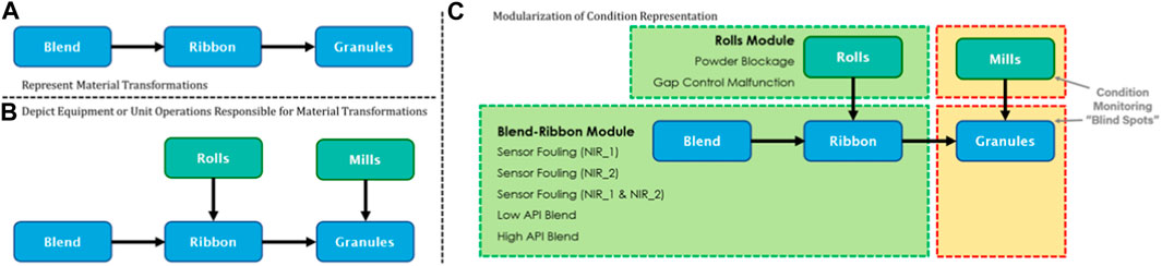
Figure 3. Representing the Condition of a Roller Compactor. (A) Representing Material Transformations. (B) Depicting Equipment and Unit Operations Responsible for Material Transformations. (C) Mapping existing CM systems to the process condition representation.

Once material transformations have been depicted, the next step is to consider the equipment conditions, which we represent as green nodes instead of blue, to visually differentiate equipment from material conditions. For the roller compactor, this would be the condition of the rolls and the mill, which respectively affect the transformation of the powder blend into a ribbon, and the ribbon into granules. Their roles in material transformations could then be captured using arrows, forming a directed graph (Roweis and Ghahramani, 1999) as shown in Figure 3B.

Similarly, for cases where more types of conditions are considered, i.e., condition of the sensors and the controllers, they could be integrated into the graph using arrows. For example, if a sensor is monitoring the ribbon, and that sensor is providing feedback to the control system of the roller compactor, then a directed arrow should connect the node depicting the condition of that sensor towards the ribbon condition node. This implies that if the sensor is malfunctioning, it could negatively impact the condition of the roll.

The graph produced during the representation stage offers an illustrated model of the condition of the roller compactor, which would have otherwise been a complicated concept to describe, and even more so to predict. With such a representation, the goal of condition monitoring could now be defined as the process of predicting the values of the equipment and condition nodes in real-time.

4.2 Modularization

Having a proper representation of the process condition enables the proper evaluation of the current visibility of the condition of the process system. For example, the WP-120 roller compactor already has existing CM systems. Previous fault detection and diagnosis efforts focused on automatically detecting powder blockage and gap control malfunction from machine data Gupta et al. (2013); Lagare et al. (2021). Moreover, efforts were ongoing to develop a CM system that can automatically discriminate material faults from sensor faults Lagare et al. (2021).

Would it be sufficient to use these CM systems autonomously? Do they offer holistic monitoring of the process condition? Having a proper representation of the process condition in Figure 3B allows the proper mapping of the existing systems on the condition representation. By looking at the location of the faults considered by the two different CM systems, it can be established that the CM system focused on detecting powder blockage and gap control malfunction is monitoring the condition of the rolls, while the other one is monitoring the condition of both the blend and the ribbon.

By properly mapping these systems as shown in Figure 3C, it becomes apparent that there is limited visibility on the full process condition—i.e., there are no systems monitoring the mills and the granules. These “blind spots,” which are marked with orange boxes in Figure 3C, thus need their own CM modules. The creation of these modules could be prioritized in the next stage of the framework—i.e., machine learning model development.

Notice that the two blind spots could also be addressed by having one condition monitoring system that covers both the mills and granules. This could certainly be the case and the actual implementation would depend on the availability of sensors or the availability of known faults. If nothing is measured from the mills and there are no known faults, then it would be impossible to have a CM system created just for the mill. As will be further explained in Section 4.3, any modular CM system would require at least one measurement variable and one fault that is localized in that module. It would be more sensible to just integrate it with the granule condition node or leave it as a blind spot. The latter would be the more flexible option because additional sensors would leave the granule module undisturbed.

As new sensors are installed, new faults could be discovered. Having the process condition modularized means that retraining the condition monitoring systems, to accommodate the additional input variables from the new sensors and the new faults to classify, is confined to only the affected module. This makes it so much more efficient in comparison to retraining a much larger singular model had the process condition not been modularized.

Because of the simplicity of the RC process condition, the modularization job was relatively straightforward; the mill condition and granule condition variables could be assigned their own separate (or combined) CM modules. However, for larger systems, this modularization problem might not be as trivial, so a proper workflow is required. This proposed workflow is shown in Figure 4 and it involves designating a central node, which must have a fault associated with it as a primary requirement. This also means that faults are always located on any one of the condition variable nodes. Otherwise, the process condition representation in Figure 3B might be incomplete and is most likely missing a condition variable.

Figure 4

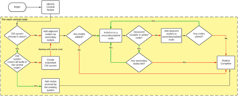
Figure 4. Modularization workflow.

If this central node also has measured variables in addition to the fault, then it can potentially stand alone as a module since it would complete the predictor and predicted variable sets for the machine learning development phase. If this central node has measured variables, then adjacent nodes need to be incorporated into the module. If the adjacent nodes still do not have measured variables, then the nodes adjacent to it would be added, repeating this process until all added nodes have a measured variable associated with them.

This modularization methodology ensures that the measured variables closest to the fault location are included in the modules. It can be reasonably expected that these variables have a higher chance of displaying signatures that can identify a fault, by comparison to other variables that are farther away. This methodology essentially filters out variables that would have added to the complexity of the machine learning task, but not necessarily improved its performance.

While the resulting modules in the RC application case study were consistent with this workflow, the simplicity of its process did not require the full extent of its features. However, this will be covered in a follow-up paper to this publication where more complicated case studies are tested using the framework.

The workflow in Figure 4 also considers the presence of existing CM systems that may or may not cover all the known faults associated with the central node. If the latter is the case, it is recommended to create a new CM system that would cover all known faults for the central node. This new system could then be treated as the primary monitoring module, while the existing one could be used as a redundant option.

4.3 ML model development

Machine learning models have recently become synonymous with neural networks. However, they are much more general than that. A machine learning model is any model that does not have to be explicitly programmed to perform a task. It assumes a general structure with a fixed set of parameters (or hyperparameters) but uses data to tune these parameters in a way that it performs the task well given the scope of the data. There are many tasks that a machine learning model could perform, and classification is a machine learning task that can be used to automate fault detection and diagnosis.

It is certainly possible to simply take all the data from a process, apply appropriate pretreatments, and use the pre-treated data to train a classification machine learning model that can classify in real-time the process condition into any of the possible conditions in the condition library.

Doing this has disadvantages: updating new sensors and new faults would require retraining a very big model; changes in the process would require training a very big model; and training a very big model would require a very large training dataset. The proposed framework addresses these issues by breaking the entire process condition representation into smaller modules; simplifying machine learning model training during initial development as well as model retraining as new sensors are installed and new faults are discovered.

In the RC example, the representation and modularization stages break down the process condition monitoring task into four smaller condition monitoring modules, each with their own condition libraries that can be used to train their own condition monitoring system. The next stage would be to train machine learning models for these modules so that the measured variables in the module can be used to predict the condition associated with the central node (or the node containing the faults) of the module.

This operation can be visualized in Figure 5, where the measured/manipulated variables in the rolls and blend-ribbon modules are used to assign a probability to each possible condition in the central node—i.e., normal, fault 1, fault 2, etc.—and a voting system will identify the one with highest probability to be the predicted condition.

Figure 5

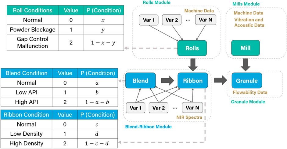
Figure 5. How CM systems work (figure showing measured and manipulated variables predicting the central nodes).

The gray broken arrows in Figure 5 indicate that the condition nodes represent discrete probability tables. When a condition monitoring module makes a prediction, it essentially assigns a value of 1.0 to the condition probability of each node that is included in the module. This is a simple concept to understand for the Rolls module since it only comprises one node. However, for the Blend-Ribbon module, it is not very straightforward, although it is still relatively simple.

Consider the list of conditions for the Blend-Ribbon module in Table 1. It Is a list that predates this proposed framework, so this list does not resemble anything like the discrete probability tables in Figure 5, which is a result of representation and modularization. If a machine learning model would be trained to classify the process among the conditions in this list, it is not obvious how these predictions could be used to update the probabilities of the condition nodes in Figure 5. To make this connection, each of the items in the condition list should assign a state to all the condition nodes that are involved in the module, if they are predicted to be the condition. For example, if Fault 1 in Table 1 is the predicted condition, then it should assign a normal state (value = 0) to the blend and ribbon condition nodes. Similarly, if Fault 4 was the predicted condition, then the blend condition and ribbon condition nodes would be assigned a value = 1, since the state of the blend is low API, which would result in a low-density state for the ribbon.

Table 1

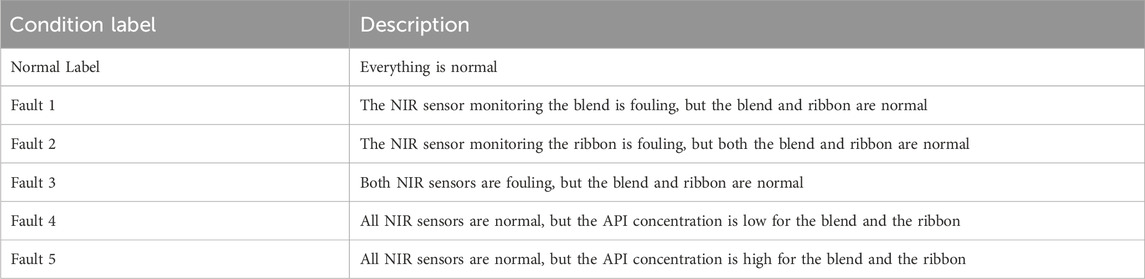
Table 1. Condition list for blend-ribbon module.

Translating the results of a modular condition monitoring system into a value for each of the nodes in the module is an important aspect of this framework. This is a requirement for mapping existing condition monitoring modules onto the process condition representation. Non-translatability could be an indication that the mapping is incorrect, and a review needs to be made of the scope of the existing system.

This translatability is a concern even if the modular system was identified as a blind spot after representation and modularization. If a module covers one or more condition nodes, it would be ideal to redefine the condition library in terms of the different states of the condition nodes that are included in the module. However, if this is impractical to do, it is mandatory to implement a translation scheme that assigns corresponding states to all the pertinent condition nodes for every predicted condition in the condition library.

4.3.1 The ML model development workflow

One of the enabling technologies of this framework is the availability of machine learning platforms that automatically suggest a machine learning algorithm for the data and the particular type of machine learning job. For condition monitoring, the machine learning job type is classification, where continuous variables are used as predictors for the fault types, which can be assigned as discrete variables (e.g., 0, 1, or 2) that correspond to each of the predicted fault types.

The machine learning platform used for the RC case study is ML.NET, Microsoft, (2022) which has the Model Builder feature that can take training data from the process, suggest the most effective machine learning algorithm, and then generate the code of the trained model that one could use for predictions. In the machine learning model development workflow shown in Supplementary Figure S1, the Model Builder feature primarily handles the “Build and Train” stage, which involves selecting the best machine learning model for the loaded data, and then training and evaluating the model. This results in a code containing the fully trained model that can be used to make predictions on real-time data. The engineer tasked with developing the CM system can then focus on preparing the data and extracting features from the data, a task that can require domain expertise Lagare et al. (2023).

A major benefit of the Model Builder feature is the accessibility of the most advanced machine learning algorithms within a single package. This promotes a streamlined workflow of model training and discrimination, which could lead to the best possible model for a given dataset. This is most useful given the evolutionary nature of the process and the corresponding condition monitoring system; the most appropriate machine learning model might change as more fault data is collected and as more faults are discovered. Having an integrated package for all machine learning models facilitates this evolution better by promoting a toolbox-oriented approach (Venkatasubramanian, 2009) to model development. This is an advantage over the widespread practice of implementing different models using different programming platforms, different languages, and different libraries; because even if a condition monitoring system developer is familiar with a certain algorithm, its limited availability on specific programming platforms and languages could discourage its inclusion into the machine learning model development workflow.

4.3.2 Data preparation

As specified in Supplementary Figure S1, training data needs pre-treatment before ML model development can begin. For this case study, it is advantageous to make the predictions robust against random fluctuations by capturing the rolling average and standard deviations. Furthermore, it is better to center and scale the data using the mean and standard deviation, Chiang et al. (2000); Yin et al. (2012); Basha et al. (2020) both of which are measured from normal operating conditions data.

This pretreatment workflow is illustrated in Supplementary Figure S2 and can be considered as part of the feature extraction step described in Supplementary Figure S1 for the ML Model Development Workflow. This workflow does not have to be followed exactly for all CM systems development jobs since the appropriate one would most likely vary on the situation, depending particularly on the data and the ML Model Development scheme that is employed. However, for the Model Builder Feature of ML.NET, this data pretreatment scheme yielded superior results across the modules in the RC case study.

4.3.3 Alternative ML development methodologies

ML.NET is very advantageous for CM systems development, as will be shown in the Results and Discussion section, and it is certainly a very convenient way for a non-expert in machine learning to harness the latest advances in the field. However, it is worth mentioning that it is not necessarily the best platform for ML model development.

If the CM systems developer can invest time in learning about probabilistic graphical modeling, particularly factor graphs, it is possible to utilize a new paradigm in ML model development called Model-based Machine Learning (MBML). Bishop, (2013) The idea behind this paradigm stems from a unifying view of machine learning where the models can be represented as a factor graph, Roweis and Ghahramani, (1999) and the ML predictions can be implemented by performing Bayesian inference on the graphs. Infer.NET is a program that can perform these inferences efficiently via message passing algorithms (Minka et al., 2018a) and has been demonstrated to be successful in running ML models that are bespoke to the applications. Braunagel et al. (2016); Vaglica et al. (2017); Minka et al. (2018b) Discussing the details of this paradigm is beyond the scope of this paper, and its possible advantages over ML.NET requires further investigation. However, the reader is directed to http://dotnet.github.io/infer for more information.

4.3.4 ML performance evaluation and novel fault detection capabilities

Condition monitoring systems are typically evaluated using fault detection rates (FDR) and false alarm rates (FAR). Chiang et al. (2000); Yin et al. (2012) In order for a classification model to be useful, fault detection rates should be close to 1 and false alarm rates need to be close to 0. One of these cannot be underperforming; a very high fault detection rate is useless if the system is in a constant state of false alarms, and a very low false alarms rate is pointless if a system is unable to detect most faults. Hence, the FDR and FAR have become standard measurements in comparing the effectiveness of different machine learning algorithms applied to condition monitoring of the same processes.

While these two metrics are included in evaluating the machine learning models developed in the RC application case study, they can be insufficient. These CM systems are meant to be utilized by a human operator, which would only happen if the latter can trust the predictions made by the former. Trusting these predictions can be tricky if the fault library is initially incomplete, as is the case for many process systems. An incomplete fault library means that the CM system would try to classify a novel fault as one of the conditions in the fault library, which can lead to an incorrect and a potentially disastrous response. Hence, it is important that novel conditions are properly detected and managed; otherwise, the operator would never be able to trust the condition predictions, even though the FDR and FAR are perfect.

Hence, two additional metrics are introduced in this study to evaluate the trained ML models: normal condition prediction certainty index and the overall prediction certainty. These proposed indices capitalize on prediction certainties as an additional layer of information that can be used to predict novel faults. More information on novel fault management and novel detection performance indices are detailed in Section 4.3.5.

4.3.5 Novel fault management

As noted above, it is imperative that a condition monitoring system employs an effective system for managing novel faults, particularly to detect them before they are properly identified. Novel fault detection practically acknowledges the limitation of the model and properly initiates intervention by the operator to detect and diagnose faults that are either novel or have data signals that have not been experienced before.

The management of novel conditions or faults is often neglected in the condition monitoring literature, but it is a very important aspect of condition monitoring systems, especially when facing the possibility of encountering faults with a very short degradation time. A proposed solution is to employ machine learning classifiers that assign scores or probabilities to the different classes; a voting mechanism would select the class with the highest probability and assign it as the predicted class. Often, this probability is merely used to get the predicted class, but this can serve as a layer of information that can aid in detecting novel conditions.

Consider the predictions made by a condition monitoring system in Figure 6. This system employs a machine learning model that has been trained to classify two conditions: normal and fault type 1 (powder blockage). So, regardless of the actual condition, it will classify either normal or fault type 1. In the figure, fault type 2 was induced at 100 s; the model does not recognize fault type 2, so it incorrectly predicts the condition to be normal. But notice the probability assigned to the condition being normal; it went from higher than 0.95, to less than 0.85. If a threshold was applied at a probability of 0.90, where any prediction that has an assigned probability less than 0.90 would be rejected, a novel condition could be deduced.

Figure 6

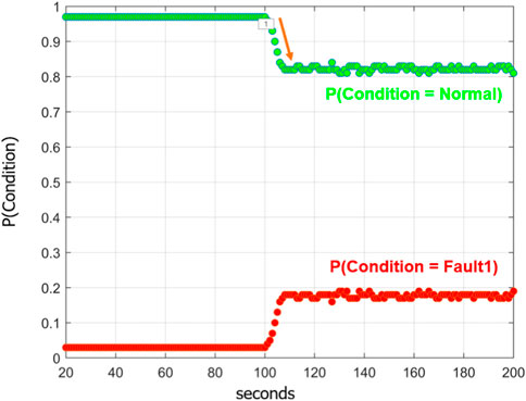
Figure 6. Test predictions of the Condition Monitoring System for Fault 2 (before the module was trained for its data signatures).

This proposed method of novel fault detection thus requires the use of machine learning classifiers that assign a score or a probability to each condition (and then uses a voting mechanism to select the condition with the highest score or probability to be the predicted condition), and that the predictions for the known conditions be higher than an assigned threshold (e.g., 0.90). The latter requirement could be challenging to accomplish especially with a very large system, but this should be remedied by the representation and modularization aspects of the proposed framework.

A full demonstration of this novel fault detection will be reported in an upcoming paper, but at this point we simply note that it is important to consider beforehand the ability of a machine learning model to detect novel faults as part of the model discrimination process during the ML model development stage of the proposed framework. Since the proposed detection scheme for novel faults relies on high prediction certainties, at least relative to a threshold, it is possible to evaluate novel fault detection capabilities based on prediction certainty criteria.

4.3.6 Novel fault detection performance indices

We propose at least two certainty indices to evaluate for novel fault detection capabilities: the normal condition certainty index and the overall prediction certainty index. These indices are computed using a threshold, which we nominally select to be 0.90. The overall prediction certainty index is calculated by counting the number of predictions that has a probability higher than the nominally selected threshold, and then dividing this by the total number of predictions. The normal condition certainty index is calculated by counting the number of normal condition predictions that have a probability higher than the nominally selected threshold, and then dividing this by the total number of normal condition predictions. These certainty indices have no regard for the accuracy of their predictions, so they need to be used in conjunction with the accuracy analytic, which is just the number of correctly predicted conditions, divided by the total number of predictions.

Computing these certainty indices effectively evaluates the ability of a machine learning model to detect novel faults. Together with fault detection rate, false alarm rate, and accuracy, these indices provide a comprehensive scheme to discriminate machine learning models during the ML model development stage of the proposed framework. Table 2 is a summary of performance indices used for model selection and their definitions.

Table 2

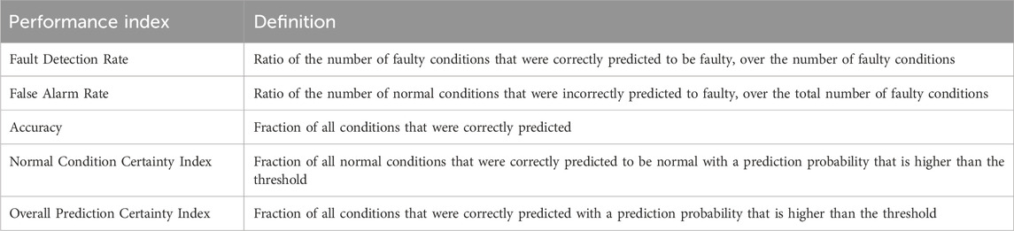
Table 2. Summary of performance indices used for machine learning model selection.

4.3.7 Updating CM modules

The discovery of new faults necessitates updating the CM system. With a framework that relies on modularization, updating entails retraining a ML model for the pertinent module. This is much more practical than the alternative, which is to retrain the entire system just to be able to add one fault to the fault library. A modularized CM system is much more practical to maintain as well. If a tablet press (TP) were to be added to the process, as it would for a dry granulation line, then this would be as simple as adding more modules after the granule condition node. A centralized system would have to retrain a new model that would now include both the RC and the TP, and this could be more expensive to do, if not impossible, to yield a high performing classifier of conditions.

4.4 Module integration

After the ML Model development stage, all the CM modules identified in Figure 3C should already have a working ML model. For the RC application case study, this means that values of the nodes depicted in Figure 5 could now be predicted in real-time. The ability of these modular systems to make reliable predictions on the values of the nodes depends on the reliability of the sensors, which require regular maintenance. When they do, the CM modules relying on those sensors to make predictions would cease to function, which would compromise the visibility of the condition nodes.

Fortunately, the directed graph (Figure 3B) that is the end-product of the representation stage in the framework can be treated as a such. As a directed graph, the condition nodes are linked by unidirectional arrows that determine their causality, which can be used to make inferences, both qualitative and quantitative. Qualitatively, for the RC case, the rolls and blend nodes both have an arrow directed to the ribbon node. This can be interpreted as the dependency of the condition of the ribbons on the condition of the blend and the condition of the rolls transforming the blend into ribbons. With these known dependencies, it is possible to make useful inferences.

4.4.1 Inferring missing condition nodes

For example, in Figure 7A, if the condition of the both the ribbon and the rolls are both unknown, but the blend was observed to be defective, then it is reasonable to infer that the ribbon might end up being defective. Likewise, in Figure 7B if the rolls are malfunctioning, the produced ribbon could be defective. If both the rolls and blend were observed to be abnormal, then the chances of the ribbon being defective is even higher, as shown in Figure 7C.

Figure 7

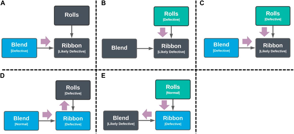
Figure 7. Reasoning scenarios of using observed nodes (blue or green colored nodes) to unobserved nodes (black nodes). (A) Inferring ribbon condition based on observed condition of the blend. (B) Inferring ribbon condition based on observed condition of rolls. (C) Inferring ribbon condition based on observed condition of rolls and blend. (D) Inferring the blend was defective since the ribbon was observed to be defective while the rolls were confirmed to be functioning normally. (E) Inferring rolls are malfunctioning since the ribbon was defective but the blend was good.

An even more interesting inference is when it goes upstream of the flow of dependencies. For example, in Figure 7D, the ribbon was observed to be defective, but the rolls were found to be working normally; it would be reasonable to infer that the blend might be the defective one. Similarly, in Figure 7E, it would be reasonable to infer that the rolls might be malfunctioning if the ribbon was found to be defective, but the blend was confirmed to be normal.

These reasoning scenarios show that the availability of a directed graph to represent the process condition is useful in cases where only some nodes are observed; one can use the observed nodes to predict the condition of the unobserved ones. In an ideal case for a fully functional CM system, all condition nodes should always be visible. However, the ability of the CM systems to “observe” the nodes depends on the performance of pertinent sensors, and sensors do experience performance drifts and regular maintenance. When these issues occur, and sensors need to be temporarily taken out of operation, it would be valuable to maintain the visibility of the process system condition, thereby ensuring that quality assurance is maintained without having to resort to a process shutdown.

4.4.2 Probabilistic programming and inference

Although the variable relationships discussed in Figure 7 are all qualitative reasonings, they can also be performed quantitatively using Bayesian inference. This makes it possible to automate the process and implement it as the fourth stage of the framework (Figure 8)—i.e., module integration.

Figure 8

Figure 8. Framework for development of condition monitoring systems.

Taking the situation in Figure 7D as an example, where the nodes represent random variables and the arrows represent their probabilistic relationships, the directed graph represents the following equation by the basic laws of probability:

$P\left(Blend,Rolls,Ribbon\right)=P\left(Rolls\right)P\left(Blend\right)P\left(Ribbon|Rolls,Blend\right)(\mathrm{Equation\; 1})$

To infer the condition of the blend, observations of the rolls and the ribbon must be utilized, which were 0 and 1 respectively since the rolls were normal and the ribbon was defective. Applying Bayes’ Rule yields:

$P\left(Blend|Roll=0,Ribbon=1\right)=\frac{P\left(Blend,Rolls=0,Ribbon=1\right)}{P\left(Rolls,Ribbon\right)}(\mathrm{Equation\; 2})$

The denominator in Equation 2 can be calculated by summing over the Blend variable from Equation 1, which yields the following equation.

$P\left(Blend|Roll=0,Ribbon=1\right)=\frac{P\left(Blend,Rolls=0,Ribbon=1\right)}{{\sum }_{Blend}P\left(Rolls=0,Ribbon=1,Blend\right)}(\mathrm{Equation\; 3})$

Substituting the numerator Equation 1 into the numerator in Equation 3 yields:

$P\left(Blend|Roll=0,Ribbon=1\right)=\frac{P\left(Rolls=0\right)P\left(Blend\right)P\left(Ribbon\left.=1\right|Rolls=0,Blend\right)}{{\sum }_{Blend}P\left(Rolls=0\right)P\left(Blend\right)P\left(Ribbon\left.=1\right|Rolls=0,Blend\right)}(\mathrm{Equation\; 4})$

Using Equation 3 posterior probabilities of the blend being normal or defective can be computed. For demonstration purposes, we can assign variables to the conditional probability tables that the nodes in Figure 7D represent, as shown in Tables 3–5. The variables $x,y,a,b,c,d,e$ represent actual probability values of the condition nodes. Hence, these conditional probability tables must be learned beforehand to perform these inferences. We can substitute these variables into Equation 4 for brevity to give Equation 5 and Equation 6 for the blend being normal or defective respectively. These probabilities could then be compared to make a prediction about the condition of the blend.

$P\left(Blend\left.=0\right|Roll=0,Ribbon=1\right)=\frac{xy\left(1-a\right)}{xy\left(1-a\right)+xy\left(1-b\right)}(\mathrm{Equation\; 5})$

$P\left(Blend\left.=1\right|Roll=0,Ribbon=1\right)=\frac{xy\left(1-b\right)}{xy\left(1-a\right)+xy\left(1-b\right)}(\mathrm{Equation\; 6})$

Table 3

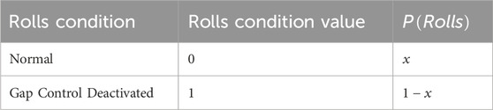
Table 3. Probability table of the rolls condition node.

Table 4

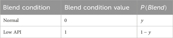
Table 4. Probability table of the blend condition node.

Table 5

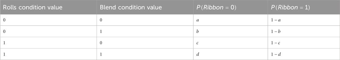
Table 5. Conditional probability table of the ribbon condition node.

The preceding development equation for the 3-node graph from Figure 7D can be applied to the full Roller Compactor representation in Figure 3B, where the following joint probability equation in Equation 7 would be used instead of Equation 1. Predicting the blend condition could then be computed by starting out with the following equation and then applying Bayes’ rule as previously outlined.

$P\left(Blend,Rolls,Ribbon,Mill,Granules\right)=P\left(Rolls\right)P\left(Blend\right)P\left(Ribbon|Rolls,Blend\right)P\left(Mill\right)P\left(Granules|Mill,Ribbon\right)(\mathrm{Equation\; 7})$

Of course, working out these equations will lead to Equation 5 and Equation 6 because the denominator in Equation 2 would now entail summing the joint probability over the blend, mill, and granules condition variables, which will lead to a value of 1 for $P\left(Mill\right)$ and $P\left(Granules|Mill,Ribbbon\right)$.

The ability to perform this type of inference even with increasing number of variables is an important modularity feature that would allow the integration of other unit operations like the tablet press, adjacent to the roller compactor. However, exact inference on graphical models is NP-hard (Dagum and Luby, 1993), and as the model gets bigger with more condition variables, exact inference can be computationally expensive and impractical for monitoring purposes.

Fortunately, inference can be performed approximately (Bishop and Nasrabadi, 2006; Bishop, 2013) through a probabilistic programming framework like Infer.NET, Minka et al. (2018a) which is the same program used for the MBML paradigm described in Section 4.3.3. Infer.NET allows a user to program the graph in Figure 7D probabilistically—i.e., the condition nodes have assigned probabilities—and perform Bayesian inference on those nodes via computationally efficient message passing algorithms Lagare et al. (2022).

4.4.3 Learning the priors

The first three stages of the framework shown in Figure 8 results in modular CM systems that ultimately convert process data from the sensors and equipment into a dataset with discrete values. If the individual nodes in RC condition model in Figure 3B were all binomial—i.e., the nodes have two possible values—then the dataset from the CM modules would resemble Figure 9, which shows that for each observation, all the condition nodes (e.g., blend, rolls, etc.) would have two possible values (0 or 1) that would correspond to its actual state (normal or faulty).

Figure 9

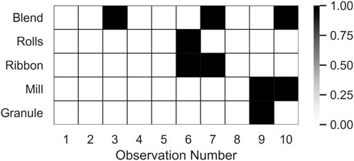
Figure 9. Data from the modular CM systems.

The collection of this discrete dataset, when all the CM modules are functional—i.e., no sensors or equipment are under maintenance—is the critical piece that can be used to learn about the ground truth of a process condition. This ground truth is illustrated in Figure 10, where each node represents a discrete probability distribution that is represented by the corresponding conditional probability tables. For simplicity, most of the nodes assume a binomial distribution to represent that the possible states could be normal or faulty. However, these nodes can be assigned a multinomial distribution to align with the typical fault library that would most likely have more than one fault type. To demonstrate this extendibility, the granules node was assigned such a distribution with three possible states.

Figure 10

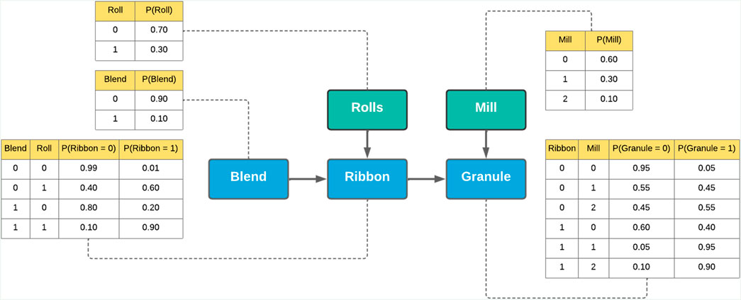
Figure 10. Sample ground truth of a process condition model.

In order to make accurate inferences on unobserved nodes based on the observed conditions of adjacent nodes, it is important to learn this ground truth. This can be done by first adding additional nodes to represent the prior probability of each of the condition nodes. With each observation from a fully functional CM system with no ongoing sensor or equipment maintenance, one can use Bayesian inference or message passing algorithms to infer the values of the prior probability nodes. This parameter learning scheme is illustrated in Figure 11.

Figure 11

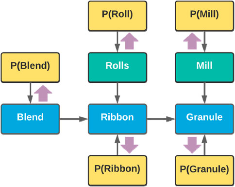
Figure 11. Learning the prior probabilities.

The size requirement of the data for learning the prior probabilities is a potential issue for integration, especially as the number of unit operations, and hence the number of condition nodes, increase. However, for the RC application case that has five condition nodes, the assumed ground truths in Figure 10 was learned after 100 observations, which is subjectively a manageable number. As shown in Figure 12, further observations only increase the certainty of the prior probabilities.

Figure 12

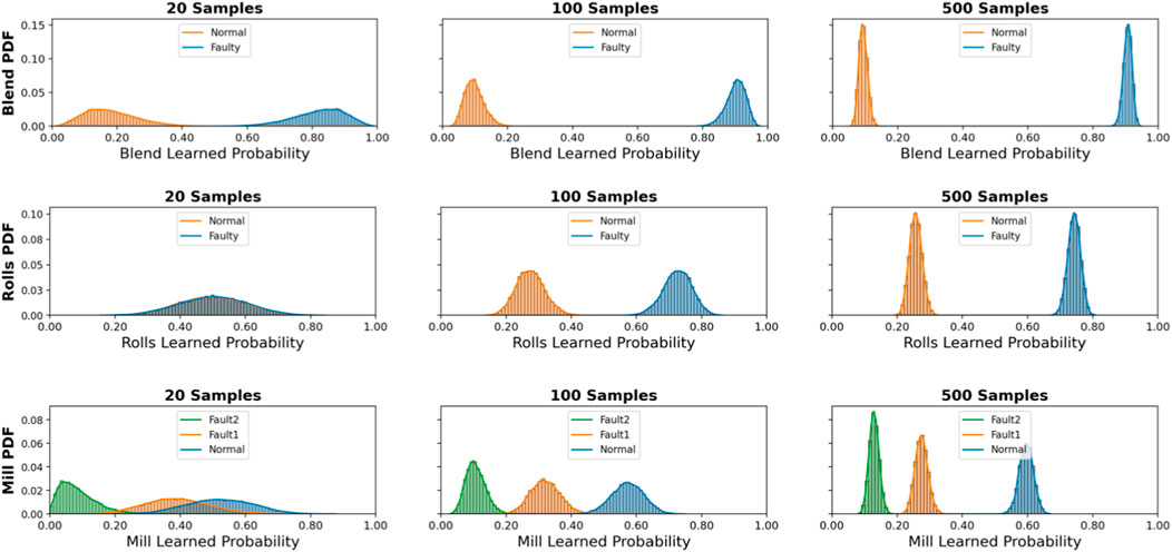
Figure 12. Parameter learning versus observations.

There will be a critical number of observations that are required to correctly learn the ground truths. This number is expected to increase as more condition nodes are integrated into the model and as more faults are added to the fault library, since it would increase the number of states in the existing condition nodes. While Bayesian inference could be performed regardless, the accuracy of those inferences can only be useful once the ground truths have been properly learned. Hence, the ability to estimate this critical number based on the current structure of the graphical model (i.e., the result of the process condition representation stage) could provide framework users a convenient way to set a target number of complete condition data from the modules, indicating when process condition graphical model could be reliably used for integration. Such investigations are important but are beyond the scope of this paper but should be addressed in future studies.

4.4.4 Enhancing decision-making and robustness

With a properly trained condition model, it would now be possible to reliably use the priors to enhance the capabilities of the CM system. An important scenario arises when the granule condition is not visible, possibly due to sensor maintenance. Since the granule condition practically pertains to the Critical-Quality-Attributes (Yu et al., 2014) of the RC operation, the inability to monitor it removes the assurance of product quality, and a process shutdown might be necessary, which can be costly.

However, with a holistic module integration scheme, quality assurance does not have to suffer during sensor maintenance. As shown in Figure 13A, it is possible to use the observations on the condition of the adjacent nodes—e.g., the ribbon and mill condition nodes—to infer the condition of the product granules. These inferences are summarized in Figure 14, where the predictions on the granule condition varies with possible observations on the ribbon and mill conditions.

Figure 13

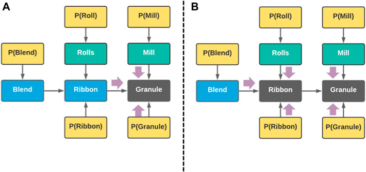
Figure 13. Product granule quality inference scenarios during sensor maintenance. (A) Inferring granule condition monitoring module under maintenance. (B) Inferring ribbon and granule condition monitoring module under maintenance.

Figure 14

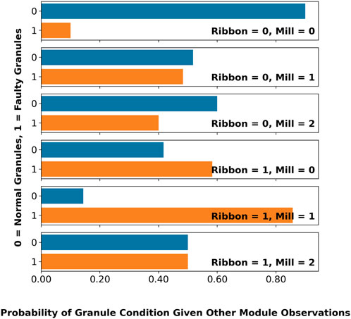
Figure 14. Inferred probabilities of granule condition based on possible conditions of the ribbon and the mill.

Furthermore, inferences are even possible with multiple unobserved nodes. In the case of Figure 13B, the ribbon node is also unobserved in addition to the granule, but the condition of the product quality could still be inferred to maintain quality assurance during operation. This is possible because the remaining observed nodes—e.g., blend, rolls, and mill—are “connected” under the d-separation (Bishop and Nasrabadi, 2006) criterion. Since the inferred condition of the granules are now dependent on the observations of three nodes instead of two, there are more possible predictions for the granule condition, which are summarized in Figure 15.

Figure 15

Figure 15. Possible granule inferences based on observations of the blend, roll, and mill.

5 Results and Discussion

The focus of this paper is to introduce the concepts underlying the framework for developing CM systems. However, even with the RC as a target application case, it is not currently possible to give a full demonstration of the framework in this paper; the development of the individual CM systems is still a work in progress. In fact, a concept of virtual sensor for monitoring granule flowability has just been recently published (Lagare et al., 2023), and a working sensor for monitoring granule properties in real-time does not exist yet. Likewise, the CM module for the mill condition also lacks a proper sensor for monitoring, and this is still ongoing research by our team.

However, two modules—e.g., rolls and blend-ribbon modules—that were identified and mapped by framework, are already prime for discussion and offer sufficient proof of the effectiveness of the framework.

5.1 Performance of modular systems

5.1.1 Roll module

The roll module mapped in Figure 3C is based on an earlier study (Gupta et al., 2013) that utilized statistics based on Principal Components Analysis (PCA) to detect abnormal conditions, but then relied on an operator to diagnose the nature of the condition based on the PCA loadings. To avoid this reliance on a skilled operator to classify the fault, ML.NET was used to select and train a machine learning model that can automatically detect and classify faulty conditions.

As illustrated in Figure 5, the rolls module can have any of the three conditions: normal, powder blockage (fault 1), or gap control malfunction (fault 2). To predict these conditions, machine data was used: roll gap, roll speed, feed screw speed, and roll pressure. These data would then be used to predict the probabilities of each possible condition of the rolls, depicted in Figure 16 as either x, y, or z; where the sum of x, y, and z equals 1.

Figure 16

Figure 16. Role of machine learning in converting data into condition probabilities.

This classification problem in machine learning is one of the pre-defined scenarios in the Model Builder feature in ML.NET; thus, reducing the task of ML development to gathering the training data, loading it to the Model Builder platform, and then getting the trained model from the platform and then further validating it with testing data (see Supplementary Figure S1).

For this supervised machine learning problem (Jordan and Mitchell, 2015), three datasets are required for training: data during normal conditions, data during powder blockage, and data during gap control malfunction. The datasets for these conditions are shown in Figure 17, which are simulated based on actual data collected by previous research (Gupta et al., 2013); the simulations of faulty data started out as normal with a fault induced at 500 s. Pretreatment of this data as described in Section 4.3.2 yields the plots shown in Figure 18, which shows the rolling means and standard deviations of the data centered around zero during normal conditions, and then deviating away as a fault is introduced.

Figure 17

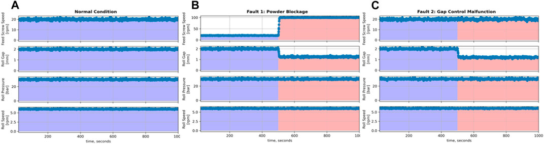
Figure 17. Simulating data on the feed screw speed, roll gap, roll pressure, and roll speed of the roller compactor. (A) Process data under normal condition. (B) Process data under powder blockage condition. (C) Process data under gap control malfunction.

Figure 18

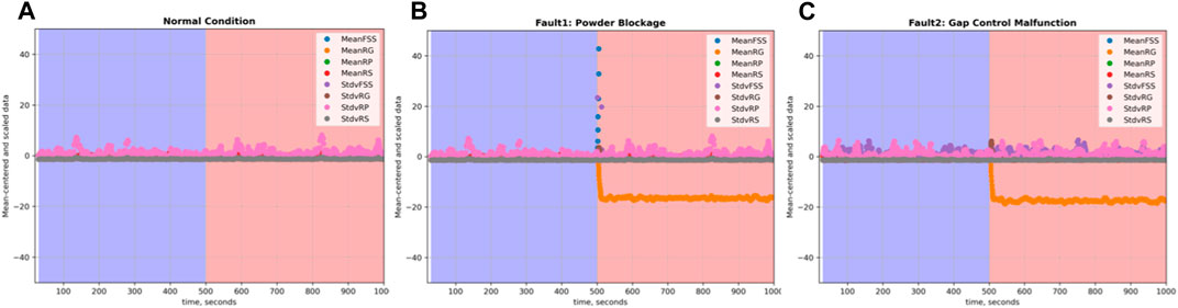
Figure 18. Mean-centered and scaled data on the Feed Screw Speed, Roll Gap, Roll Pressure, and Roll Speed of the Roller Compactor under (A) Normal Condition, (B) Powder Blockage Condition, and (C) Gap Control Malfunction.

After this series of data preparation steps, the training data was loaded into the Model Builder feature of ML.NET, which recommended a gradient-boosted decision tree called LightGBM (Ke et al., 2017) to be the best model among the 52 trained machine learning models that it considered. For additional information on gradient-boosted decision trees (GBDT), see the Supplementary Appendix section.

As shown in Figure 19, the recommended model did not only correctly predict the actual conditions of the testing data, but it also predicted the onset of the fault with minimal delay and with high prediction probabilities. High probabilities can be interpreted as high prediction certainty, which can be useful for adding useful capabilities to the model like novel fault management. Management of novel faults will be discussed in more detail in Section 4.3.5.

Figure 19

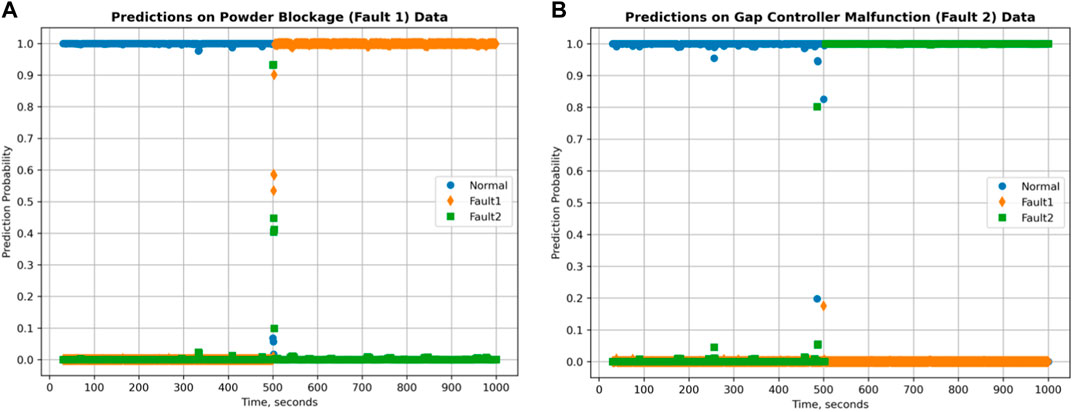
Figure 19. Predictions on roller compactor process condition for (A) powder blockage, and for (B) gap control malfunction.

Visually, the prediction performances look good, which can be further quantified into appropriate classification performance evaluation metrics such as accuracy, fault detection rate, and false alarm rates. Chiang et al. (2000); Yin et al. (2012) In order to further evaluate potential capabilities of the trained models to detect novel faults, additional metrics were computed: normal condition prediction certainty index and the overall prediction certainty index. The computation of these indices is discussed in more detail in Section 4.3.5.

Table 6 shows the computed measures of performance for the Rolls module. It shows the effectiveness of the current ML Model development methodology employed in developing the CM system for the module, which is practically perfect.

Table 6

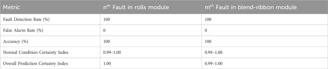
Table 6. Performance of the CM system developed for the rolls and blend-ribbon module.

5.1.2 Blend- module

Just like the rolls module, the blend-ribbon module was part of an earlier fault detection and diagnosis study on the RC, which focused on two NIR sensors monitoring the RC, as shown in Figure 20. Dual NIR monitoring of the RC allows simultaneous monitoring of the powder blend in the feed hopper and the ribbon coming out between the rolls. A chemometric model can then be used to predict the composition and density of the powder or the compact based on the NIR spectra readings. Roggo et al. (2007); Stranzinger et al. (2021) This offers redundancy in measurements on API measurements in the feed and the ribbon, while giving unique information on the density of the ribbon and the feed.

Figure 20

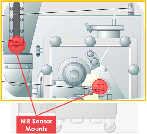
Figure 20. Dual NIR monitoring of the RC.

Creating a fault detection and diagnosis system practically attempted to investigate if dual NIR monitoring allows the discrimination between sensor faults and material faults. NIR sensors are prone to drift and fouling issues; if the composition and density estimates from the sensors indicate the blend or the ribbon is off-specification, is it possible to rule out the sensor being faulty?

Framing this in a CM system development problem requires the creation of a fault library, which has the following faults:

1. The NIR sensor monitoring the blend is fouling, but the blend and ribbon are normal.

2. The NIR sensor monitoring the ribbon is fouling, but the blend and ribbon are normal.

3. Both NIR sensors are fouling, but the blend and ribbon are normal.

4. All NIR sensors are normal, but API blend is too low.

5. All NIR sensors are normal, but the API blend is too high.

Datasets for each of these faults were simulated and shown in the following figures. The plots in these figures show the time series estimates of density and composition from the NIR readings, as well as the true values of the density and composition. For all these fault datasets, the condition starts at normal, and the corresponding fault is induced at 400 s. The data for the first two faults shows the true values of composition and density staying constant, but the estimates from either the first or second NIR sensor drop to a lower steady-state value, as shown in Figures 21A, B respectively. Figure 21C shows the dataset for the third fault, when the both the first and second NIR sensors drop to a lower steady-state, while the true values are constant.

Figure 21

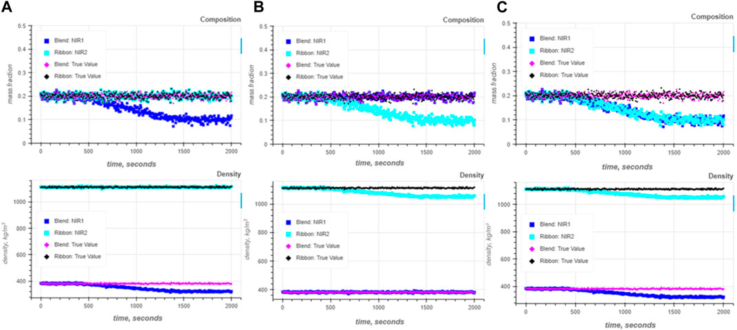
Figure 21. Simulating different sensor fouling scenarios with normal blend and ribbon conditions during roller compaction operation. (A) NIR sensor monitoring the blend is fouling. (B) NIR sensor monitoring the ribbon is fouling. (C) Both NIR sensors are fouling.

The fourth and fifth faults all have both the NIR sensors working well, and something really is wrong with the material. The datasets for these faults show how the true values of the composition, and consequently the density, changes to a new steady-state value. Figure 22A shows the NIR sensors capturing the drop in the density and API composition of the blend and the ribbon, while Figure 22B shows the NIR sensors capturing the increase in the density and API composition. For both the datasets, notice the slight delay in the density and composition changes in the ribbon relative to the blend. This delay was intentionally included to account for the residence time distribution of the blend particles from the location of the first NIR sensor that is monitoring the powder blend, to the second NIR sensor that is monitoring the ribbon.

Figure 22

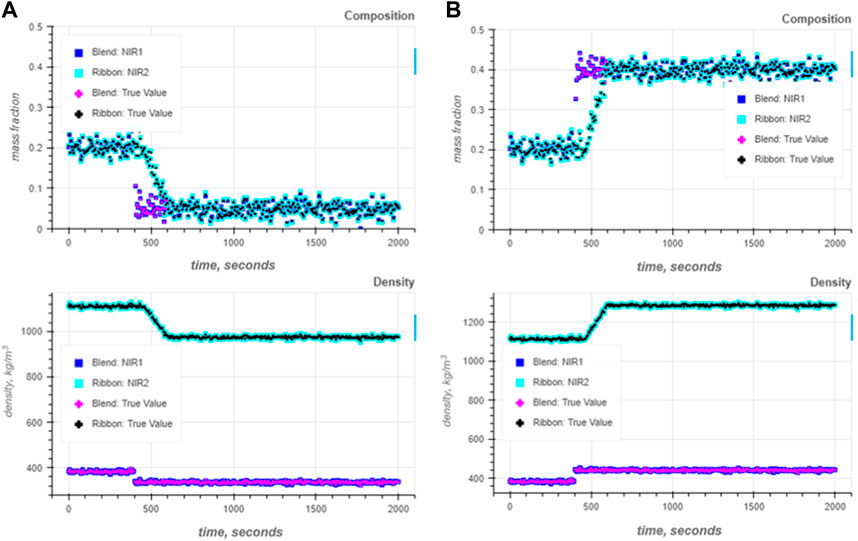
Figure 22. Simulating faulty RC operating conditions under normal functionality of NIR sensors. (A) Simulating API concentration being too low in the blend and the ribbon. (B) Simulating API concentration being too high in the blend and the ribbon.

Similar to the workflow discussed in Section 5.1.1, the data preparation scheme illustrated in Supplementary Figure S2 was applied to all the datasets. Using only the NIR sensor readings (i.e., not including the true values of density and composition), the datasets were entered into Model Builder in ML.NET, which suggested Gradient-boosted Decision Trees (Ke et al., 2017) for the classification job, just like the Rolls Module.

The prediction performance for the test data involving all known conditions for the module are shown in Figure 23. Each of these plots represent a time-series of scores that the machine learning classifier assigned for each of the conditions in the fault library (e.g., normal, Fault 1, Fault 2, etc.), and the predicted condition would be the one with the highest score. Ideally, the predicted condition would be the true condition at that time step, and the prediction score would be high, as this could be interpreted as the prediction certainty.

Figure 23

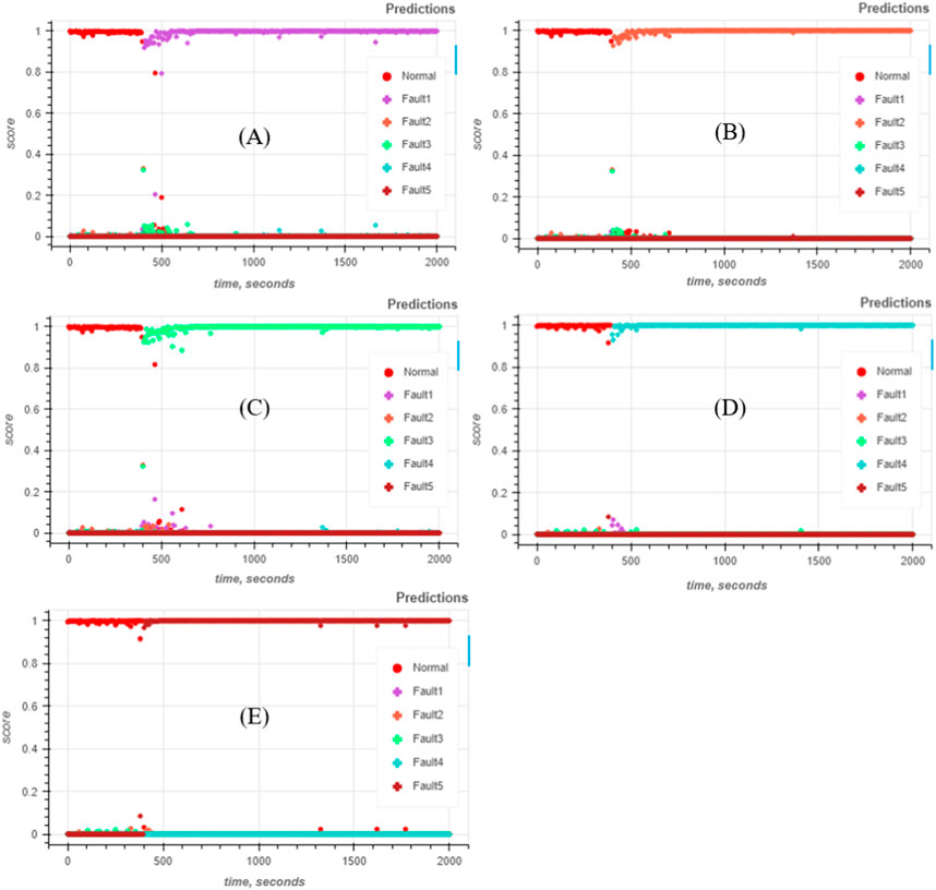
Figure 23. Predicting RC process conditions under different scenarios. (A) Fault 1: NIR-1 is fouling. (B) Fault 2: NIR-2 is fouling. (C) Fault 3: NIR-1 and NIR-2 are fouling. (D) Fault 4: Low API, normal NIR sensors. (E) Fault 5: High API, normal NIR sensors.

It can be seen from Figure 23 that the classifier correctly predicted the condition to be normal at time steps before 400 s. Moreover, the prediction score is close to 1.0, which can be interpreted as having a prediction certainty close to 100%. When the corresponding faults are induced at 400 s, the classifier assigned the highest score to the appropriate fault, with a prediction certainty that is still close to 100%. There is also minimal delay in the prediction change, as the corresponding faults were correctly predicted a few seconds after they were induced.

The prediction performances of the machine learning classifiers trained for this module is summarized in Table 6; just like the Rolls Module, the classifiers performed perfectly based on the performance measurement indices listed in Table 2.

6 Conclusion

We introduced a framework that enables the practical development of effective condition monitoring systems. It involves four stages: representation, modularization, machine learning model development, and module integration. Representation uses process knowledge to create a graph that represents the condition of the process, and modularization uses this graph to break down the process into more manageable modules, which would have a smaller set of faults to classify and a smaller input of variables to consider. High-performance machine learning models could then be trained for each module so they would be able to correctly predict the condition of that respective module in real-time and potentially detect novel fault conditions. Finally, since modularization was based on a directed graph that was created based on the causal relationships of the process condition components, they can be integrated holistically. This allows important inferences to be made that can aid in decision-making and improve the robustness of the process, especially during maintenance involving one or more sensors or equipment. The leveraging of available process knowledge to boost the condition monitoring performance of machine learning models is what makes this framework unique, and applying this approach to other problems could prove beneficial.

Ultimately, this framework promotes modularization, which can not only drive down costs of developing condition monitoring systems, but also for maintaining it. As new faults are added to the fault library, a centralized system would have to retrain a very large model, while a modular system would only need to retrain the pertinent module. Furthermore, as new components of the process are added, the modular system would only need to add more modules and at most would only modify a few modules, whereas a non-modular system would need to start from scratch every time.

Data availability statement

The original contributions presented in the study are included in the article/Supplementary Material, further inquiries can be directed to the corresponding author.

Author contributions

RL: Conceptualization, Data curation, Formal Analysis, Investigation, Methodology, Project administration, Software, Validation, Visualization, Writing–original draft, Writing–review and editing. MG: Funding acquisition, Resources, Supervision, Writing–review and editing. ZN: Funding acquisition, Resources, Supervision, Writing–review and editing. GR: Funding acquisition, Resources, Supervision, Writing–review and editing.

Funding

The author(s) declare financial support was received for the research, authorship, and/or publication of this article. This work was supported by the NSF under grant #2140452.

Conflict of interest

The authors declare that the research was conducted in the absence of any commercial or financial relationships that could be construed as a potential conflict of interest.

Publisher’s note

All claims expressed in this article are solely those of the authors and do not necessarily represent those of their affiliated organizations, or those of the publisher, the editors and the reviewers. Any product that may be evaluated in this article, or claim that may be made by its manufacturer, is not guaranteed or endorsed by the publisher.

Supplementary material

The Supplementary Material for this article can be found online at: https://www.frontiersin.org/articles/10.3389/fenrg.2024.1351665/full#supplementary-material

References

Akkisetty, P. K., Lee, U., Reklaitis, G. V., and Venkatasubramanian, V. (2010). Population balance model-based hybrid neural network for a pharmaceutical milling process. J. Pharm. Innov. 5, 161–168. doi:10.1007/s12247-010-9090-2

CrossRef Full Text | Google Scholar

Basha, N., Ziyan Sheriff, M., Kravaris, C., Nounou, H., and Nounou, M. (2020). Multiclass data classification using fault detection-based techniques. Comput. Chem. Eng. 136, 106786. doi:10.1016/j.compchemeng.2020.106786

CrossRef Full Text | Google Scholar

Becker-Hardt, M., 2018. The compaction people continuous dry granulation by roller compaction an introduction to the Alexanderwerk roller compaction process.

Google Scholar

Bishop, C. M. (2013). Model-based machine learning. Philosophical Trans. R. Soc. A Math. Phys. Eng. Sci. 371, 20120222. doi:10.1098/rsta.2012.0222

PubMed Abstract | CrossRef Full Text | Google Scholar

Bishop, C. M., and Nasrabadi, N. M. (2006). Pattern recognition and machine learning. Springer.

Google Scholar

Braunagel, C., Geisler, D., Stolzmann, W., Rosenstiel, W., and Kasneci, E. (2016). “On the necessity of adaptive eye movement classification in conditionally automated driving scenarios,” in Proceedings of the Ninth Biennial ACM Symposium on Eye Tracking Research & Applications, 19–26.

CrossRef Full Text | Google Scholar

Chen, T. (2014). Introduction to boosted trees. Univ. Wash. Comput. Sci. 22, 115.

Google Scholar

Chiang, L. H., Russell, E. L., and Braatz, R. D. (2000). Fault detection and diagnosis in industrial systems. Springer Science & Business Media.

Google Scholar

Dagum, P., and Luby, M. (1993). Approximating probabilistic inference in Bayesian belief networks is NP-hard. Artif. Intell. 60, 141–153. doi:10.1016/0004-3702(93)90036-B

CrossRef Full Text | Google Scholar

Friedman, J. H. (2001). Greedy function approximation: a gradient boosting machine. Ann. Statistics 29, 1189–1232. doi:10.1214/aos/1013203451

CrossRef Full Text | Google Scholar

Ganesh, S., Su, Q., Vo, L. B. D., Pepka, N., Rentz, B., Vann, L., et al. (2020). Design of condition-based maintenance framework for process operations management in pharmaceutical continuous manufacturing. Int. J. Pharm. 587, 119621. doi:10.1016/j.ijpharm.2020.119621

PubMed Abstract | CrossRef Full Text | Google Scholar

Gupta, A., Giridhar, A., Venkatasubramanian, V., and Reklaitis, G. V. (2013). Intelligent alarm management applied to continuous pharmaceutical tablet manufacturing: an integrated approach. Ind. Eng. Chem. Res. 52, 12357–12368. doi:10.1021/ie3035042

CrossRef Full Text | Google Scholar

Hastie, T., Tibshirani, R., and Friedman, J. (2009). “Ensemble learning,” in The elements of statistical learning: data mining, inference, and prediction. Editors T. Hastie, R. Tibshirani, and J. Friedman (New York, New York, NY: Springer), 605–624. doi:10.1007/978-0-387-84858-7_16

CrossRef Full Text | Google Scholar

Iri, M., Aoki, K., O’shima, E., and Matsuyama, H. (1979). An algorithm for diagnosis of system failures in the chemical process. Comput. Chem. Enyinerriny 3, 489–493. doi:10.1016/0098-1354(79)80079-4

CrossRef Full Text | Google Scholar

Jordan, M. I., and Mitchell, T. M. (2015). Machine learning: trends, perspectives, and prospects. Science 349 (1979), 255–260. doi:10.1126/science.aaa8415

PubMed Abstract | CrossRef Full Text | Google Scholar

Kazemi, P., Khalid, M. H., Szlek, J., Mirtič, A., Reynolds, G. K., Jachowicz, R., et al. (2016). Computational intelligence modeling of granule size distribution for oscillating milling. Powder Technol. 301, 1252–1258. doi:10.1016/j.powtec.2016.07.046

CrossRef Full Text | Google Scholar

Ke, G., Meng, Q., Finley, T., Wang, T., Chen, W., Ma, W., et al. (2017). Lightgbm: a highly efficient gradient boosting decision tree. Adv. Neural Inf. Process Syst. 30.

Google Scholar

Lagare, R., Sheriff, M. Z., Nagy, Z., and Reklaitis, G. (2021). “The use of hybrid modeling schemes in the development of a probabilistic condition monitoring system for a continuous drug product manufacturing process,” in 2021 AIChE Annual Meeting (AIChE).

Google Scholar

Lagare, R. B., Huang, Y.-S., Bush, C.O.-J., Young, K. L., Rosario, A. C. A., Gonzalez, M., et al. (2023). Developing a virtual flowability sensor for monitoring a pharmaceutical dry granulation line. J. Pharm. Sci. 112, 1427–1439. doi:10.1016/j.xphs.2023.01.009

PubMed Abstract | CrossRef Full Text | Google Scholar

Lagare, R. B., Sheriff, M. Z., Gonzalez, M., Nagy, Z., and Reklaitis, G. V. (2022). A comprehensive framework for the modular development of condition monitoring systems for a continuous dry granulation line. Comput. Aided Chem. Eng. 49, 1543–1548. doi:10.1016/B978-0-323-85159-6.50257-8

CrossRef Full Text | Google Scholar

Lee, S. L., O’Connor, T. F., Yang, X., Cruz, C. N., Chatterjee, S., Madurawe, R. D., et al. (2015). Modernizing pharmaceutical manufacturing: from batch to continuous production. J. Pharm. Innov. 10, 191–199. doi:10.1007/s12247-015-9215-8

CrossRef Full Text | Google Scholar

LightGBM (2023). LightGBM 4.1.0.99 documentation. Microsoft Corporation.

Google Scholar

Microsoft (2022). What is ML.NET and how does it work?. Available at: https://learn.microsoft.com/en-us/dotnet/machine-learning/how-does-mldotnet-work?WT.mc_id=dotnet-35129-website (Accessed January 12, 22).

Google Scholar

Minka, T., Cleven, R., and Zaykov, Y. (2018a). Trueskill 2: an improved bayesian skill rating system. Tech. Rep.

Google Scholar

Minka, T., Winn, J. M., Guiver, J. P., Zaykov, Y., Fabian, D., and Bronskill, J., 2018b. Infer.NET 0.3.

Google Scholar

Natekin, A. (2020). Topic 10. Gradient boosting | kaggle. Available at: https://www.kaggle.com/code/kashnitsky/topic-10-gradient-boosting/notebook (Accessed May 10, 23).

Google Scholar

Roggo, Y., Chalus, P., Maurer, L., Lema-Martinez, C., Edmond, A., and Jent, N. (2007). A review of near infrared spectroscopy and chemometrics in pharmaceutical technologies. J. Pharm. Biomed. Anal. 44, 683–700. doi:10.1016/j.jpba.2007.03.023

PubMed Abstract | CrossRef Full Text | Google Scholar

Rogozhnikov, A., 2016. Gradient Boosting explained [demonstration]. Available at: http://arogozhnikov.github.io/2016/06/24/gradient_boosting_explained.html (Accessed 10.May.23).

Google Scholar

Roweis, S., and Ghahramani, Z. (1999). A unifying review of linear Gaussian models. Neural comput. 11, 305–345. doi:10.1162/089976699300016674

PubMed Abstract | CrossRef Full Text | Google Scholar

Schenkendorf, R. (2016). Supporting the shift towards continuous pharmaceutical manufacturing by condition monitoring Conference on Control and Fault-Tolerant Systems, SysTol 2016-November, 593–598. doi:10.1109/SYSTOL.2016.7739813

CrossRef Full Text | Google Scholar

Stranzinger, S., Markl, D., Khinast, J. G., and Paudel, A. (2021). Review of sensing technologies for measuring powder density variations during pharmaceutical solid dosage form manufacturing. TrAC - Trends Anal. Chem. 135, 116147. doi:10.1016/j.trac.2020.116147

CrossRef Full Text | Google Scholar

Su, Q., Ganesh, S., Moreno, M., Bommireddy, Y., Gonzalez, M., Reklaitis, G. V., et al. (2019). A perspective on Quality-by-Control (QbC) in pharmaceutical continuous manufacturing. Comput. Chem. Eng. 125, 216–231. doi:10.1016/j.compchemeng.2019.03.001

PubMed Abstract | CrossRef Full Text | Google Scholar

Sun, W. J., Rantanen, J., and Sun, C. C. (2018). Ribbon density and milling parameters that determine fines fraction in a dry granulation. Powder Technol. 338, 162–167. doi:10.1016/j.powtec.2018.07.009

CrossRef Full Text | Google Scholar

Vaglica, V., Sajeva, M., McGough, H. N., Hutchison, D., Russo, C., Gordon, A. D., et al. (2017). Monitoring internet trade to inform species conservation actions. Endanger. Species Res. 32, 223–235. doi:10.3354/esr00803

CrossRef Full Text | Google Scholar

van Wyk, A. (2018). An overview of LightGBM. Available at: https://www.avanwyk.com/an-overview-of-lightgbm/ (Accessed May 10, 23).

Google Scholar

Vedam, H., and Venkatasubramanian, V. (1997). Signed digraph based multiple fault diagnosis. Comput. Chem. Eng. 21, S655–S660. doi:10.1016/s0098-1354(97)00124-5

CrossRef Full Text | Google Scholar

Venkatasubramanian, V. (2009). Drowning in data: informatics and modeling challenges in a data-rich networked world. AIChE J. 55, 2–8. doi:10.1002/aic.11756

CrossRef Full Text | Google Scholar

Venkatasubramanian, V. (2011). Systemic failures: challenges and opportunities in risk management in complex systems. AIChE J. 57, 2–9. doi:10.1002/aic.12495

CrossRef Full Text | Google Scholar

Venkatasubramanian, V., Rengaswamy, R., and Kavuri, S. N. (2003a). A review of process fault detection and diagnosis Part II: qualitative models and search strategies. Comput. Chem. Eng. 27, 313–326. doi:10.1016/s0098-1354(02)00161-8

CrossRef Full Text | Google Scholar

Venkatasubramanian, V., Rengaswamy, R., Yin, K., and Kavuri, S. N. (2003b). A review of process fault detection and diagnosis: Part I: quantitative model-based methods. Comput. Chem. Eng. 27, 293–311. doi:10.1016/s0098-1354(02)00160-6

CrossRef Full Text | Google Scholar

Yin, S., Ding, S. X., Haghani, A., Hao, H., and Zhang, P. (2012). A comparison study of basic data-driven fault diagnosis and process monitoring methods on the benchmark Tennessee Eastman process. J. Process Control 22, 1567–1581. doi:10.1016/j.jprocont.2012.06.009

CrossRef Full Text | Google Scholar

Yu, L. X., Amidon, G., Khan, M. A., Hoag, S. W., Polli, J., Raju, G. K., et al. (2014). Understanding pharmaceutical quality by design. AAPS J. 16, 771–783. doi:10.1208/s12248-014-9598-3

PubMed Abstract | CrossRef Full Text | Google Scholar