A DC fault current fast-computing method of MMC-HVDC grid with short circuit protection equipment

1 Introduction

Compared to point-to-point transmission, the multi-terminal high-voltage direct current (HVDC) grid offers several advantages, such as connecting a larger number of renewable energy sources and provides higher power supply reliability, making it a key area of focus in future grid research (Li et al., 2021). The voltage-source converter (VSC) technologies, specifically those based on the modular multilevel converter (MMC), are rapidly expanding the applications of high-voltage direct current (Shu et al., 2023). VSC-HVDC systems, which utilize MMC, are particularly well-suited for multi-terminal DC (MTDC) systems due to their ability to flexibly control current direction and redistribute power between terminals (An et al., 2017).

However, the issue of DC short circuit fault protection poses a significant challenge and acts as a major obstacle to the development and implementation of multi-terminal HVDC grids with overhead lines. When a DC grid experiences a short-circuit fault, it is necessary to insert short circuit protection equipment into the fault path to limit the rising rate and break current of the fault current, as well as isolate the short circuit fault (Ahmad et al., 2022; Zhang et al., 2022). The presence of SCPE within a multi-terminal MMC-HVDC grid adds complexity to the system, making it highly challenging to accurately calculate fault currents and analyze the performance of SCPE within the grid.

The Electromagnetic-transient-type (EMT) simulation tool is capable of accurately simulating the performance of an HVDC grid under normal or fault conditions (H. Saad et al., 2013). The EMT model of the MMC converter accurately represents thousands of IGBT switching events simultaneously. A multi-terminal HVDC system based on MMC consists of multiple MMC converters (Stepanov et al., 2021). However, simulating a multi-terminal MMC-HVDC grid using EMT model requires a lot of computing resources and is time-consuming, because the multi-terminal MMC-HVDC grid is a time-variable and nonlinear circuit. To improve computational efficiency, several numerical computing approaches have been developed. The literature (LI et al., 2017a) provides a detailed analysis of MMC arm fault current before the converter blocks during a pole-to-pole fault in a single-terminal HVDC system. Additionally, an RLC equivalent circuit model of the MMC under short fault conditions has been reported by (Belda et al., 2018; Yang et al., 2018).

Moreover, the overhead line is approximated as an R-L circuit in (Li et al., 2016; Li et al., 2022). Based on the RLC equivalent circuit model of MMC and the R-L circuit of overhead lines, a linear RLC model of MMC-HVDC grid has been established in literature (Li et al., 2017b) for calculating short-circuit currents. This model is referred to as the RLC equivalent circuit in this paper and has made significant progress in the calculation of short-circuit current by representing the time-variable-nonlinear circuit of the multi-terminal HVDC grid as an RLC linear model. In addition to the RLC equivalent circuit, the literature (Li et al., 2017a) proposed a general time-domain numerical calculation method for analyzing the pole-to-pole short-circuit fault of the pseudo-bipolar multi-terminal MMC-HVDC grid. Furthermore, the literature (Ning et al., 2019; Ye et al., 2021) introduced how to utilize this method to calculate and analyze pole-to-pole and pole-to-ground short-circuit faults of bipolar multi-terminal MMC-HVDC grids, respectively.

The conventional time-domain numerical calculation method can be divided into two steps. The first step is to establish the state equation set or the differential equation set of the RLC equivalent circuit of the MMC-HVDC grid by using Kirchhoff’s Voltage Law (KVL), Kirchhoff’s Current Law (KCL), and V A Relation (VAR). The second step is solving the equation to obtain the transient value of the fault current of the multi-terminal MMC-HVDC grid. However, despite being an important progress, the general short-circuit current calculation method of a DC grid presents several problems that need to be addressed. Please note that in the following section, the term “DC grid” specifically refers to the MMC-HVDC grid.

1) It is challenging to write the state equation set or differential equation set for the RLC equivalent circuit due to the involvement of multiple matrix calculations, making the writing process complex and cumbersome. To address this limitation, this paper presents a systematic formulation of the differential equation set.

2) If the structure of the multi-terminal DC grid is a ring, the number of equations is identical to that of the state variables in the RLC equivalent circuit. In this case, one can easily use MATLAB to solve the equations and predict the short-circuit current curves. However, if the structure is radial or hybrid, there is a virtual node in the RLC equivalent circuit, resulting in fewer equations than state variables. It becomes difficult to obtain the transient solution of the equations. Therefore, this paper proposes a novel Y-Delta transformation in the s-domain to develop an approach that eliminates the virtual node in a complex DC grid, including the ring, radial, and hybrid topologies.

In the short-circuit fault current generic calculation method based on short-circuit equivalent RLC model of the DC grid, although the SCPEs have been equipped in the DC grid, these have to be ignored since it is difficult to model the SCPEs. In this case, this method is mainly used to analyze and evaluate the development of fault currents after short-circuiting faults in DC grids without considering the effect of SCPEs, resulting in bigger analysis errors. In order to improve the analyzing accuracy, a short-circuit fault current calculation method of DC grid with SCPE is developed in this paper.

In this paper, the SCPEs are classified into three categories: fault current limiter (FCL) (Safaei et al., 2020), current limiting circuit breaker (CLCB), and DC circuit breaker (DCCB). The protection scheme for short-circuit faults in the DC grid is divided into three options: FCL + DCCB scheme, DCCB scheme, or only CLCB scheme. However, regardless of the chosen protection scheme, establishing a short-circuit fault equivalent model for DC grids with SCPEs is challenging due to the presence of solid-state switches, mechanical ultra-fast disconnectors (UFD), and metal-oxide arresters (MOA) in the SCPEs.

In the literature (Xu et al., 2019), an improved general calculation method is presented for calculating the DC fault current of a DC grid with hybrid FCL. The CLCB integrates isolating fault and limiting fault currents into a single device, reducing the cost of SCPE. According to the current limiting mechanism, the published short circuit protection equipment for the MTDC grid can be divided into MOA-type current limiting circuit breaker (CLCB) (Hedayati and Jovcic, 2018; Song et al., 2019), inductance type CLCB (Heidary et al., 2020; Wang et al., 2020) and capacitor type CLCB (Wu et al., 2020; Wu et al., 2022; Zhang et al., 2023).

Although there are several types of CLCBs, a canonical voltage source model is proposed in this paper to describe their external electrical characteristic. Importantly, this model can also be used to describe the external characteristics of other protection schemes employed in the DC grid, such as FCL + DCCB schemes or only DCCB schemes. By utilizing the canonical voltage source model of SCPEs, along with the RLC equivalent circuit of MMC and the RL equivalent circuit of the overhead line, the short-circuit fault equivalent model of the DC grids with SCPEs can be transformed into a linear circuit.

Hence, based on three big progresses, a fault current fast-computing method of MMC-HVDC grid with SCPE is proposed. This method is designed to handle various structures of DC grids with SCPEs and offers several advantages, including generality, ease of implementation, and fast computation. So, this method helps design and quickly screen and evaluate the topology, configuration scheme and timing logic of the SCPEs. In this paper, the proposed calculation method analyzes and compares the performance of three typical CLCBs.

This paper is organized as follows: A systematic formulation of the differential equation set of DC grid and eliminating virtual node approach for a radial DC grid are respectively proposed in Section 2 and Section 3. Section 4 establishes a canonical voltage source model of CLCBs to describe the external electrical characteristics of three typical CLCBs. The short circuit fault current calculation method of the DC grid with CLCB is developed in Section 5, and its computing accuracy is validated in Section 6. Section 7 analyses and compares the performances of three typical CLCBs by the proposed method, and the conclusion is introduced in Section 8.

2 Formulation of the differential equation set

2.1 RLC equivalent circuit of MTDC grid

In this paper, a four-terminal DC grid system is taken as an example, as shown in Figure 1A. The system consists of four VSCs, referred to as VSC₁, VSC₂, VSC₃, and VSC₄. There are four pairs of overhead lines, and their RLC equivalent circuit model (Li et al., 2017b) is shown in Figure 1B for short-circuit fault current calculation. According to (Belda et al., 2018; Yang et al., 2018), MMC converters can be represented by an RLC equivalent circuit under short-circuit faults. In this model, a series RLC branch is used to represent the VSC_i, which includes an internal resistance R_i, limiting current inductance L_i and discharging capacitance C_i, where i = 1,2,3,4. According to transmission line theory (Li et al., 2016), a pair of overhead line is modeled as an RL series circuit, with R_ij and L_ij representing the overhead line between VSC_i and VSC_j. The nodes $n_i^{+}/n_i^{-}$ representnthe positive/negative pole of VSC_i.

Figure 1

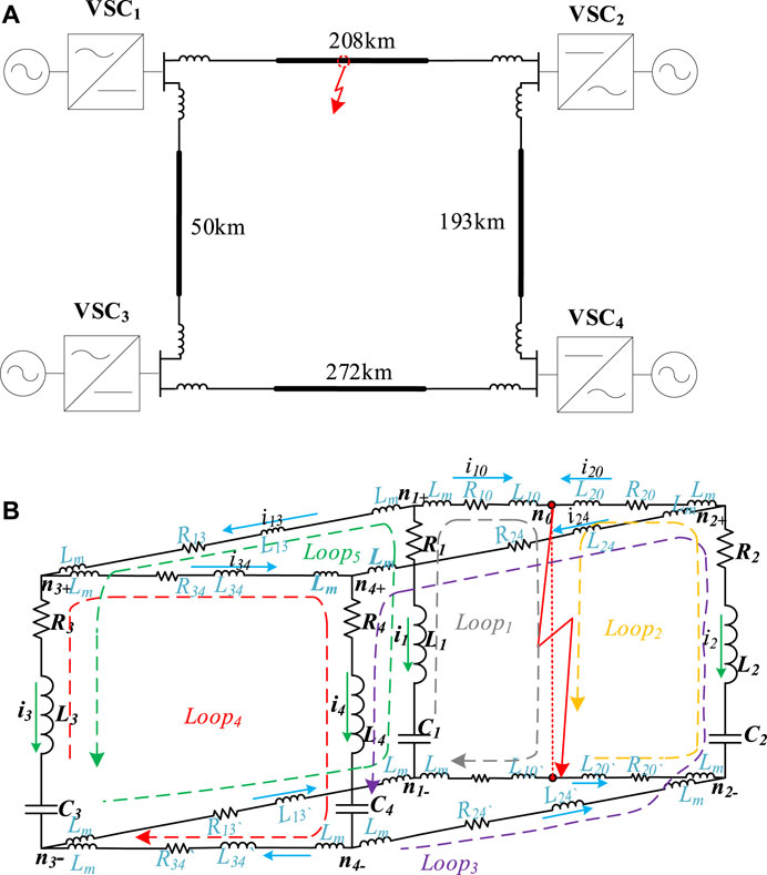
Figure 1. (A) four-terminal DC grid; (B) RLC equivalent circuit.

To establish the RLC equivalent circuit, it is assumed that a short-circuit fault occurs in the middle position of the power transmission line between VSC₁ and VSC₂. So, the number of pairs of overhead lines increases from four to five. Node n₀ is the fault point in Figure 1B, and R₁₀/₂₀ and L₁₀/₂₀ are the equivalent resistance and inductance of the overhead line between nodes n₁/₂ and n₀. The parameter calculation method for this model has been developed in (Li et al., 2017a).

2.2 Systematic formulation of the loop equations

In the RLC equivalent circuit, the circular arrows indicate the orientations of the loops chosen for writing the KVL equation. We conceive of fictitious circulating loop currents, with references given by the loop orientations. Examination of the RLC equivalent circuit shows that these loop currents are identical with the branch currents i₁, i₂, i₃, i₄ and i₅, which are the currents through the equivalent inductances L₁₀, L₂₀, L₂₄, L₃₄, and L₁₃. So, these loop currents are the state variable of the equivalent inductances of the overhead lines.

On the other hand, the voltages (u_c1, u_c2, u_c3 and u_c4) across the discharging capacitance C₁, C₂, C₃, and C₄ are also another set of state variables. To obtain a compact state equation, the loop currents rector i, the capacitance voltages rector u and its current rector i_c are defined as follows,

$\begin{array}{l}\mathit{i}={\left[i_1,i_2,i_3,i_4,i_5\right]}_{b=5}^T\\ {\mathit{i}}_{\mathit{c}}={\left[i_{c1},i_{c2},{i_c}_3,{i_c}_4\right]}_{n=4}^T\\ \mathit{u}={\left[u_{c1},u_{c2},u_{c3},u_{c4}\right]}_{n=4}^T\end{array}(1)$

By using KVL and VAR, the loop current equation can be obtained in matrix form,

$\mathbf{A}\times \mathit{u}=\mathbf{R}\times \mathit{i}+\mathbf{L}\times \dot{\mathit{i}}(2)$

Where A is an incidence matrix, R and L are parameter matrices, referred to respectively as the resistance matrix and the inductance matrix, which will be introduced later.

2.3 Incidence and parameter matrix

2.3.1 The incidence matrix A

For an RLC equivalent circuit, if there are n capacitors and b pairs of overhead lines, an incidence matrix A = [a_ij] is an n×b rectangular matrix. In this paper, the RLC equivalent circuit shown in Figure 1A will be taken as an example to introduce how to form the incidence matrix A = [a_ij].

Firstly, it is necessary to draw an oriented graph of the RLC equivalent circuit. The oriented graph associated with the RLC equivalent circuit in Figure 1A is illustrated in Figure 2A. Each node is associated with a discharging capacitor. For example, the capacitance C_i is repressed as node n_i, where i = 1, 2, 3, 4. Each branch is associated with a pair of overhead lines, and its orientation is identical to the assumed current flow. The five pairs of overhead lines are expressed as b₁, b₂, b₃, b₄ and b₅, respectively, in Figure 2A.

Figure 2

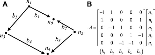
Figure 2. Oriented graph and its incidence matrix: (A) oriented graph (B) Incidence matrix.

Based on the oriented graph, the elements of incidence matrix A have the following values (Li et al., 2017b):

a_ij = 1, if branch j is incident at node i and oriented away from it; a_ij = −1, if branch j is incident at node i and oriented toward it; a_ij = 0, if branch j is not incident at node i. For the oriented graph shown in Figure 2A, the incidence matrix A is shown in Figure 2B.

2.3.2 Parameter matrices of R and L

In this paper, a systematic formulation approach for the parameter matrices of R and L is also proposed as follows. By relating parameter matrices to the RLC equivalent, the elements of the parameter matrices can be obtained using the following straightforward way.

Each term on the main diagonal is the sum of the resistance/inductance value of the branches on the corresponding loop. Each off-diagonal term is plus or minus the resistance/inductance value of branches common between two loops. The sign is positive if the loop currents traverse the common branch with the same orientation, and negative if they traverse the common branch with opposite orientations. Verify the R parameter matrix for the example by using this method.

$\begin{array}{c}\mathbf{R}=\left[\begin{array}{ccccc}{R}_1+2R_{10}& 0& 0& 0& R_1\\ 0& R_2+2R_{20}& R_2& 0& 0\\ 0& R_2& R_2+R_4+2R_{24}& R_4& 0\\ 0& 0& R_4& R_3+R_4+2R_{34}& -R_3\\ R_1& 0& 0& -R_3& R_1+R_3+2R_{13}\end{array}\right]\left[\begin{array}{l}Loop1-i_1\\ Loop2-i_2\\ Loop3-i_3\\ Loop4-i_4\\ Loop5-i_5\end{array}\right]\\ \left[\begin{array}{ccccc}{i}_1& i_2& i_3& i_4& i_5\end{array}\right]\end{array}(3)$

2.4 Systematic formulation of the node equation

In Figure 1B, four capacitances, such as C₁, C₂, C₃ and C₄, are associated with four independent capacitance-voltage state variables. On the other hand, although there are fourteen inductances, there are only five independent inductance current state variables since each independent loop corresponds to a unique independent inductance (Balabanian and Bickart, 1969). Therefore, the RLC equivalent circuit consists of nine state variables, but the Eq. 2 include only five loop current equations. Thus, it is necessary to write the remaining four equations for the state variables.

Application of KCL, the node current equations for nodes n₁, n₂, n₃ and n₄ can be written as

${\mathit{i}}_{\mathit{c}}=-{\mathbf{A}}^{\mathbf{T}}\mathit{i}(4)$

It is observed from the Eq. 4 that the capacitance current is not an independent state variable, which the independent inductance current state variables can express.

According to the constraint relationship of the capacitance voltage and current through each VSC equivalent circuit, their constraint equations are written as

${\dot{\mathit{u}}}_{\mathit{c}}=\mathbf{C}{\mathit{i}}_{\mathit{c}},\mathbf{C}=\left[c_{ij}\right],c_{ij}=\left\{\begin{array}{l}1/C_i,i=j\\ 0,i\ne j\end{array}\right.(5)$

Where C is a diagonal matrix.

Substituting the equation Eq. 4 into Eq. 5, we can get the node equation,

${\dot{\mathit{u}}}_{\mathit{c}}=\mathbf{P}\times \mathit{i},\mathbf{P}=-\mathbf{C}{\mathbf{A}}^{\mathbf{T}}(6)$

The final differential equation set are given as

$\left\{\begin{array}{l}\mathbf{A}\times \mathit{u}=\mathbf{R}\times \mathit{i}+\mathbf{L}\times \dot{\mathit{i}}\\ {\dot{\mathit{u}}}_{\mathit{c}}=\mathbf{P}\times \mathit{i}\end{array}\right.(7)$

By using the Eq. 7, the DC short fault currents of MTDC grid can be promptly and accurately calculated.

3 Eliminating virtual node approach for a radial DC grid

There are three general topologies of DC grid, referred to as the ring, radial, and hybrid topologies. According to the definition of node attributes (Li et al., 2017a), nodes n₁, n₂, n₃, and n₄ are real nodes, but node n₅ is defined as a virtual node in the radial shown in Figure 3 because it is not connected to any VSC. This virtual node will result in an important issue. The number of the differential equations of Eq. 7 will be less than that of state variables in the RLC equivalent circuit, which forms an underdetermined equation set. The reason is that we cannot find any constraint equation of the virtual node voltage and it’s current. An eliminating virtual node approach has been investigated using the Y-Delta transformation (Alexander and Sadiku, 2013) theory in this section for this type of DC grid with a virtual node.

Figure 3

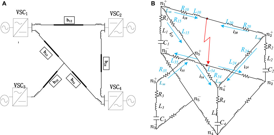
Figure 3. A radial four-terminal DC grid with virtual node and its equivalent circuit: (A) A radial four-terminal DC grid; (B) RLC equivalent circuit.

3.1 Y-Delta Transformation in the s-domain

Figure 4A shows the equivalent circuit of Y-Delta transformation in the s-domain for the virtual node n₅ in Figure 3, which is a time-domain circuit. There are two circuits named interior and exterior circuit, respectively. The interior circuit is a Why-type circuit, and the exterior circuit is its Delta-type equivalent circuit. In the s-domain circuit, an inductance L is expressed as an inductance L series with a voltage source L× i (0), where i (0) is the initial current value through the inductance L. The resistance R shares an identical form in the time domain.

Figure 4

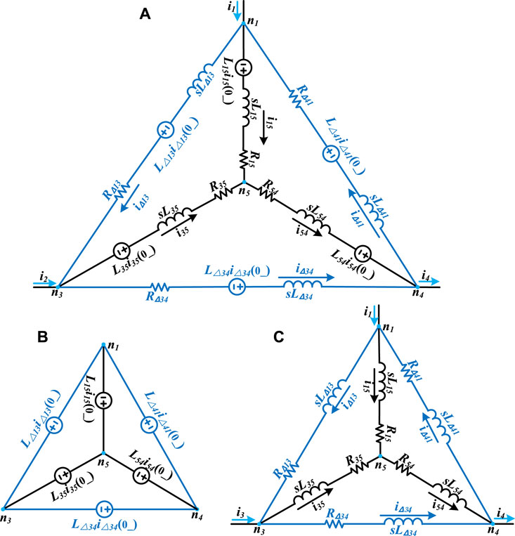
Figure 4. (A) Equivalent circuit of Y-Delta Transformation for the virtual node n5. (B) Natural response circuit (C) Force response circuit.

In order to determine the parameters of the Delta equivalent circuit, labelled as L_Δ, R_∆ and i_Δ, a circuit complete response can be broken into the natural response and the forced response (Alexander and Sadiku, 2013). Therefore, the circuit shown in Figure 4A can also be separated into the natural and forced response circuits, as shown in Figures 4B,C.

For the natural circuit shown in Figure 4B, the resistance R and inductance L are considered short circuits, because the input currents i₁, i₂ and i₃ are zero. By using KVL, the inductance current initial value of the Delta equivalent circuit can be obtained as,

$\left\{\begin{array}{l}{i}_{\Delta 41}\left(0_{-}\right)=-\frac{L_{15}{i}_{15}\left(0_{-}\right)+L_{54}{i}_{45}\left(0_{-}\right)}{L_{\Delta 41}}\\ i_{\Delta 34}\left(0_{-}\right)=\frac{L_{35}{i}_{35}\left(0_{-}\right)+L_{54}{i}_{54}\left(0_{-}\right)}{L_{\Delta 34}}\\ i_{\Delta 13}\left(0_{-}\right)=\frac{L_{15}{i}_{15}\left(0_{-}\right)-L_{35}{i}_{35}\left(0_{-}\right)}{L_{\Delta 13}}\end{array}\right.(8)$

For the force circuit shown in Figure 4C, all voltage sources can be considered short circuits since the initial value of inductance current equals zero. By using the conversion rule for Wye to Delta (Alexander and Sadiku, 2013), the following formula can be obtained,

$\left\{\begin{array}{l}{R}_{\Delta 13}+{sL}_{\Delta 13}=\frac{\left(R_{15}+s{L}_{15}\right)\left(R_{35}+s{L}_{35}\right)}{\left(R_{45}+s{L}_{45}\right)}+\left(R_{35}+s{L}_{35}\right)+\left(R_{15}+s{L}_{15}\right)\\ R_{\Delta 34}+{sL}_{\Delta 34}=\frac{\left(R_{35}+s{L}_{35}\right)\left(R_{45}+s{L}_{45}\right)}{\left(R_{15}+s{L}_{15}\right)}+\left(R_{35}+s{L}_{35}\right)+\left(R_{45}+s{L}_{45}\right)\\ R_{\Delta 41}+{sL}_{\Delta 41}=\frac{\left(R_{15}+s{L}_{15}\right)\left(R_{45}+s{L}_{45}\right)}{\left(R_{35}+s{L}_{35}\right)}+\left(R_{15}+s{L}_{15}\right)+\left(R_{45}+s{L}_{45}\right)\end{array}\right.(9)$

In DC grid, the equivalent resistance of an overhead line is much bigger than the equivalent inductance, Eq. 9 can be simplified, and the R and L expressions of the Delta equivalent circuit can be written as.

$\left\{\begin{array}{l}{R}_{\Delta 13}\approx \frac{R_{15}{R}_{35}}{R_{45}}+R_{35}+R_{15},L_{\Delta 13}\approx L_{35}+L_{15}\\ R_{\Delta 34}\approx \frac{R_{35}{R}_{45}}{R_{15}}+R_{35}+R_{45},L_{\Delta 34}\approx L_{35}+L_{45}\\ R_{\Delta 41}\approx \frac{R_{35}{R}_{45}}{R_{35}}+R_{15}+R_{45},L_{\Delta 41}\approx L_{15}+L_{45}\end{array}\right.(10)$

3.2 Equivalent circuit without virtual node

By using the proposed Y-Delta transformation in the s-domain, the virtual node n₅ in the radial four-terminal dc grid shown in Figure 3 can be eliminated, obtaining its equivalent circuit without virtual node, as shown in Figure 5. In this equivalent circuit, there is not any virtual node. So, one can use the proposed systematic formulation of the differential equation set developed in Section 2 to write its differential equation set.

Figure 5

Figure 5. Equivalent circuit without virtual node.

4 Canonical voltage source model of CLCB

According to the current limiting mechanism, the published DC circuit breaker with current limiting function can be divided into three types: MOA type CLCB, inductance type CLCB, and capacitor type CLCB, referred to respectively as MOA-CLCB, inductance-CLCB, and capacitor-CLCB. Although there are several types of CLCB, this paper proposes a canonical voltage source model, as shown in Figure 6A, to describe their external electrical characteristics. In the CLCB topology, MOA is generally employed to provide different voltages counteracting the fault current (Mohammadi et al., 2021).

Figure 6

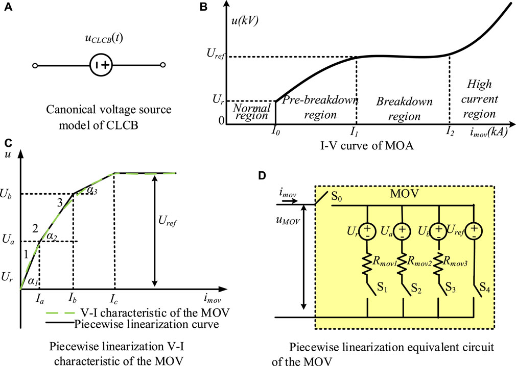
Figure 6. Canonical voltage source model of CLCB, I-V curve of MOA and its piecewise linear equivalent circuit: (A) Canonical voltage source model of CLCB. (B) I-V curve of MOA. (C) Piecewise linearization V-I characteristic of the MOV. (D) Piecewise linearization equivalent circuit of the MOV.

4.1 Piecewise linear model of MOA

Figure 6B shows a typical I-V characteristic curve of MOA, which is generally separated into four regions: the normal operational region, pre-breakdown region, breakdown region, and high current region (Martinez and Durbak, 2005). There are two voltage parameters, U_r is the rated voltage and U_ref is the reference voltage.

In CLCB, MOA is utilized to clamp the maximum to U_ref and dissipate the energy of fault current. It is difficult to analyze a CLCB circuit because MOA is a nonlinear circuit element. A piece-wise linear I-V curve of MOA, as shown in Figure 6C, is used for the pre-breakdown region and breakdown region to simplify analysis of CLCB circuit, since it is allowed to operate in the normal operational region, pre-breakdown region and breakdown region.

As shown in Figure 6C, four piece straight lines are used to describe the I-V curve, and its equivalent circuit is depicted in Figure 6D. When the MOA operates in the normal operational region, the current flowing through it is approximately several mA, it can be considered as an open circuit. Consequently, the switch S₀ remains open in the equivalent circuit. If U_r ≦ u_moa < U_a, both switches of S₀ and S₁ close, but the switches of S₂, S₃, and S₄ remain open. In this scenario, the equivalent circuit is a voltage source U_r series with the resistor R_a. Hence, the piecewise linear model of MOA can be respectively expressed as.

$R_{mov}=\left\{\begin{array}{l}{R}_{mov0}=\infty ,u_{mov}\le U_r,S_0=off\\ R_{mov1}=tg{\alpha }_1,U_r<u_{mov}\le U_a,S_0/S_1=on\\ R_{mov2}=tg{\alpha }_2,U_a<u_{mov}\le U_b,S_0/S_2=on\\ R_{mov3}=tg{\alpha }_3,U_b<u_{mov}\le U_{ref},S_0/S_3=on\\ R_{mov4}=0,u_{mov}>U_{ref},S_0/S_4=on\end{array}\right.(11)$

$\left\{\begin{array}{l}{i}_{mov}=\left\{\begin{array}{l}0,u_{mov}\le U_r\\ \left(u_{mov}-U_r\right)/R_{mov1},U_r<u_{mov}\le U_a\\ \left(u_{mov}-U_a\right)/R_{mov2}+I_a,U_a<u_{mov}\le U_b\\ \left(u_{mov}-U_b\right)/R_{mov3}+I_b,U_b<u_{mov}\le U_{ref}\end{array}\right.\\ u_{mov}=U_{ref},u_{mov}>U_{ref}\end{array}\right.(12)$

4.2 Modelling of inductance-CLCB

Figure 7A illustrates an inductive-CLCB circuit [21]. The circuit consists of L₁, which functions as the limiting current inductor of the VSC and serves as the primary side of the transformer, and L₂, which acts as the secondary side. Under normal conditions, IGBT T₁, T₃ and UFD₁ are turned on to the normal current to flow through L₁-T₁-UFD₁-T₃, as indicated by the blue dotted line in Figure 7A. In this case, there is no current flowing through L₂, because it is a high impedance branch compared with the turned on T₁ branch. The sequential control strategy of inductive-CLCB is illustrated in Figure 7A. According to the strategy, the modelling process of inductance-CLCB will be developed as follows.

Figure 7

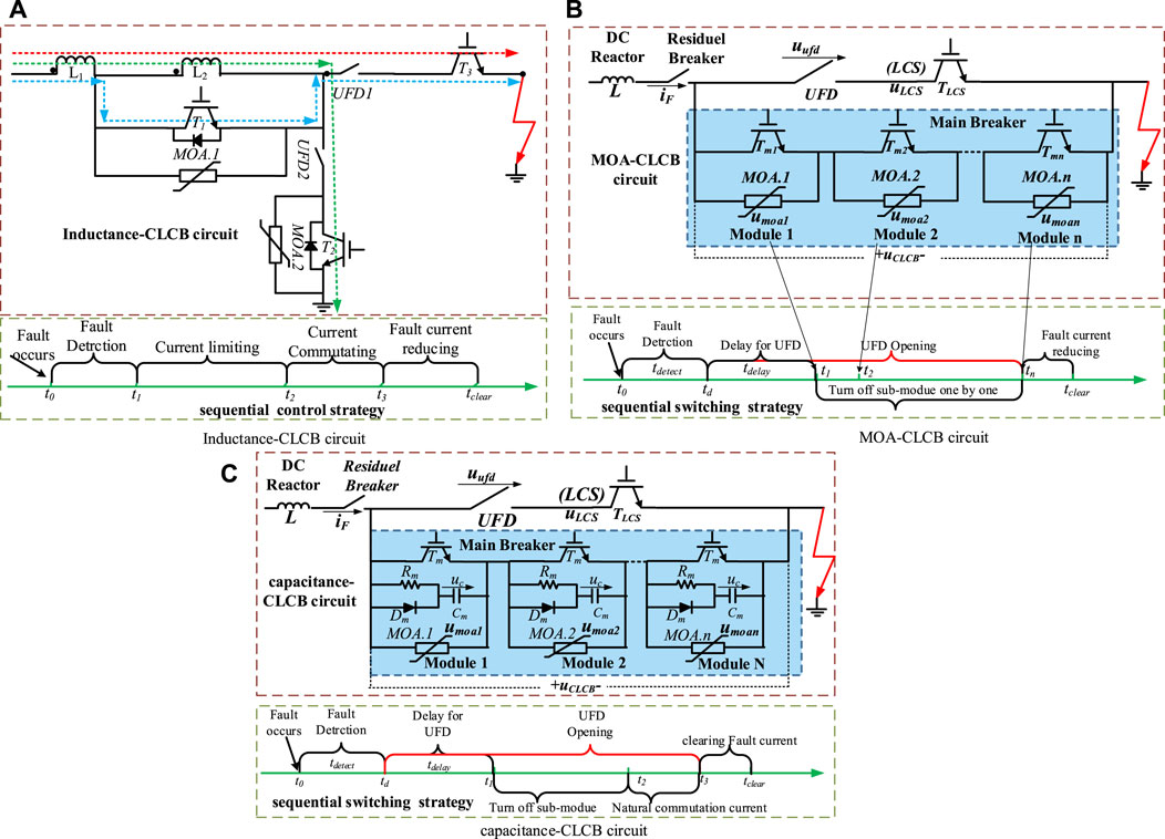
Figure 7. Three typical CLCBs CLCB and its sequential control strategy: (A) Inductance-CLCB circuit. (B) MOA-CLCB circuit. (C) Capacitance-CLCB.

Assuming a short-circuit fault occurs at time t₀, the inductance-CLCB does not operation in this interval due to the delay in the detecting signal. As a result, the fault current follows the same path as in the normal condition.

4.2.1 Current stepping interval (t₁∼t₂)

At t₁, the CLCB receives the break signal, and lets IGBT T₁ be turned on, resulting in the fault current being forced to flow through the coupling inductor L₂. At the same time, UFD₂ also receives a close signal and starts to close in preparation for the active short circuit operation.

When the coupling inductor L₂ is inserted into the circuit, the current through L₂ will experience a step from its initial value of zero. This sudden change in current will result in an extremely high overvoltage, which can potentially damage IGBTs T₁. Therefore, it is necessary to parallel MOA.1 with L₂ to limit the amplitude of the overvoltage and dissipate its energy. The equivalent circuit is depicted in Figure 8A. The voltage across L₂ is equals the voltage u_moa.1 of the MOA.1. Hence, the current through L₂ can be calculated by,

$i_{L2}\left(t\right)=\frac{1}{L_2}{\int }_{t_1}^{t_2}{u}_{moa.1}dt(13)$

Figure 8

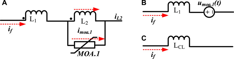
Figure 8. Equivalent circuit of inductance-CLCB: (A) equivalent circuit of (t₁∼t₂). (B) Simplified equivalent circuit of (t₁∼t₂). (C) equivalent circuit of (t₂∼t₃).

In this interval, the equivalent circuit of the CLCB is L₁ in series with a voltage source u_moa.1, as shown in Figure 8B. The CLCB voltage in this interval is

$u_{CLCB}=L_1\frac{d{i}_f}{dt}+u_{moa.1}(14)$

At t₂, two inductances L₁ and L₂ share an identical current. By using constant-flux-linkage theorem, i_L2 (t₂) can be determined

$i_{L2}\left(t_2\right)=i_{L1}\left(t_2\right)=\frac{L_1{i}_{L1}\left(t_1\right)}{L_1+L_2+2m}(15)$

Where m is the mutual coefficient, and i_L1 (t₁) is the current value through L₁ before the IGBT T₁ is turned on.

4.2.2 Inductive current limiting interval (t₂∼t₃)

Since L₁ and L₂ share identical current at t₂, no current passes through MOA.1, resulting in that MOA.1 opening. Therefore, the fault current only flows through L₁ and L₂ and the equivalent circuit of CLCB is shown in Figure 8C, and L_CL is the decoupled equivalent inductance of L₁ and L₂. L_CL and voltage u_CLCB (t) across the CLCB can be calculated.

$\left\{\begin{array}{l}{L}_{CL}=L_1+L_2+2m\\ u_{CLCB}\left(t\right)=L_{CL}\frac{d{i}_f}{dt}\end{array}\right.(16)$

4.2.3 Current shifting by active short-circuit (t₃∼t₄)

At t₃, UFD₂ has been closed completely, T₂ is turned on and UFD₁ opens. As a result, the CLCB circuit forms a low impedance ground branch, consisting of L₂, UFD₂ and T₂. This creates a new current flow path, represented by the green dotted line in Figure 7A. Hence, the equivalent circuit and voltage u_CLCB(t) expression are identical to the inductive current limiting interval.

4.2.4 MOV current limiting interval (t₄∼t₅)

At t₄, T₂ is turned off to force the fault current to pass through MOA.2. So that, u_CLCB(t) can be calculated by

$u_{CLCB}=L_{CL}\frac{d{i}_f}{dt}+u_{moa.2}\left(t\right)(17)$

Since the reference voltage U_ref of MOA.2 is approximately 1.5 times the DC voltage source U_dc of VSC, MOA.2 is utilized to provide different voltages that counteract the fault current (Mohammadi et al., 2021). At t₄, the fault current will be reduced to zero.

Based on the above modelling process, the voltage u_CLCB(t) across CLCB can be written as a united form as the followings

$u_{CLCB}\left(t\right)=\left\{\begin{array}{l}0\left(t_0\le t<t_1\right)\\ L_{cL}\frac{d{i}_f}{dt}+u_{moa.1}\left(t_1\le t<t_2\right)\\ L_{cL}\frac{d{i}_f}{dt}\left(t_2\le t<t_4\right)\\ L_{cL}\frac{d{i}_f}{dt}+u_{moa.2}\left(t\right)\left(t_4\le t<t_5\right)\end{array}\right.(18)$

Therefore, the external electrical characteristic of Inductance-CLCB can be modelled as a time-variable voltage source shown in Figure 6A, and u_CLCB can be calculated by Eq. 18.

4.3 Modelling of sequential MOA-CLCB

Figure 7B shows the MOA-CLCB circuit, proposed by ABB (Mohammadi et al., 2021). It consists of two paths referred to as LCS and main breaker. Under normal conditions, the current is allowed to pass through the LCS path. However, while a short circuit fault occurs, all IGBTs in the main breaker path are turned on to force the fault current to pass through the main breaker, comprised of several identical modules paralleled with MOA. Once the main breaker establishes a conducting path, the UFD will be opened (Mohammadi et al., 2021). When the UFD complete open operation, all IGBTs in the main breaker path are turned off in the conventional switching strategy, and then the fault current is reduced to zero. However, this conventional switching strategy can result in a high voltage.

It is noted that the UFD is a special element with non-linear-time variable characteristics, which has two moving contactors. When the contactors begin to separate, the distance between the two contactors increases linearly with time (Skarby and Steiger, 2013; Hedayati and Jovcic, 2017). By utilizing this non-linear-time variable characteristic, a sequential switching strategy of IGBTs in the main breaker was proposed, as shown in Figure 7B. This strategy aims to reduce the peak fault current, overvoltage, and fault clearance time, and is referred to as sequential MOA-CLCB (Hedayati and Jovcic, 2018; Song et al., 2019).

At t₀, a short circuit fault occurs, and the fault current flows through the LCS path. At t_d, let all IGBTs (T_m1∼T_mn) in these sub-modules be turned on to form a new fault current path. During the interval [t_d, t₁], the fault current commutates from the LCS path to the main breaker, and u_CLCB is about zero.

At t₁, let IGBT T_m1 be on to force the fault current to pass through MOA.1. Hence, u_CLCB is identical to the MOA.1 voltage, expressed as

$u_{CLCB}\left(t\right)=u_{moa.1},\left(t_1\le t<t_2\right)(19)$

At t₂, T_m2 is turned on and u_CLCB (t) can be written as

$u_{CLCB}\left(t\right)=u_{moa.1}+u_{moa.2},\left(t_2\le t<t_3\right)(20)$

The rest can be done in the same manner. Hence, the voltage u_CLCB across the sequential MOA-CLCB is written as a canonical form, such as

$u_{CLCB}\left(t\right)=\left\{\begin{array}{l}{u}_{moa.1}\left(t_1\le t<t_2\right)\\ u_{moa.1}+u_{moa.2}\left(t_2\le t<t_3\right)\\ ⋮\\ u_{moa.1}+u_{moa.2}+\cdots +u_{moa.n}\left(t_n\le t<t_m\right)\end{array}\right.(21)$

4.4 Modelling of capacitance-CLCB

Figure 7C shows the capacitance-CLCB circuit and its switching strategy [24]. At t₀, the MTDC grid experiences a short circuit fault. At t_d, the MDTC grid detects the short circuit fault and sends a break command to capacitance-CLCB. Firstly, all IGBTs Tm in the main breaker branch is turned on to form the fault current transfer path. After that, the LCS branch receives the turn-off drive signal, and the UFD starts to open to commutate the fault current from the LCS branch to the main breaker. So, during the interval [t₀, t₁], the voltage u_CLCB across the capacitance-CLCB is approximately equal to zero.

At t₁, all IGBTs T_m is turned off, so that the fault current is forced to transfer to the capacitance C_m through freewheeling diodes D_m. So that C_m begins to be charged by the fault current, and the voltage across the capacitances starts to increase from its initial value of zero. Hence, the voltage u_CLCB is.

$u_{CLCB}\left(t\right)=\frac{N}{C_m}{\displaystyle \underset{t_1}{\overset{t}{\int }}}{i}_{F}dt,t_1\le t<t_2(22)$

Where N is the number of sub-modules in the main breaker.

At time t₂, the voltage of C_m is charged to be equal to the rated voltage U_r of MOA, and the part of the fault current will pass through the MOA. Hence, the voltage u_CLCB(t) is

$u_{CLCB}\left(t\right)=N\left(U_r+\frac{1}{C_m}{\displaystyle \underset{t_2}{\overset{t}{\int }}}\left(i_F\left(t\right)-i_{moa}\left(t\right)\right)dt\right)t_2\le t<t_3(23)$

At t₃, the voltage of C_m is equal to the reference voltage U_ref of MOA, and MOA acts as a voltage source. Hence, the voltage u_CLCB is

$u_{CLCB}\left(t\right)=N\cdot U_{ref}{t}_3\le t<t_{clear}(24)$

Based on above modelling process, the voltage u_CLCB(t) can be written as a united form as the followings

$u_{CLCB}\left(t\right)=\left\{\begin{array}{l}0\left(t_0\le t<t_1\right)\\ \frac{N}{C_m}{\displaystyle \underset{t_1}{\overset{t}{\int }}}{i}_{F}dt\left(t_1\le t<t_2\right)\\ N\left(U_r+\frac{1}{C}{\displaystyle \underset{t_2}{\overset{t}{\int }}}\left(i_F\left(t\right)-i_{moa}\left(t\right)\right)dt\right)\left(t_2\le t<t_3\right)\\ u_{CLCB}\left(t\right)=N\cdot U_{ref}\left(t_3<t<t_{clear}\right)\end{array}\right.(25)$

In this section, the models of three typical CLCBs have been established, and the main contributions are the following. A canonical voltage source model, shown in Figure 6A, is proposed to describe the external electrical characteristic of the three typical CLCBs. The voltage source expressions are developed and shown in Eqs 18, 21, 25.

5 Short circuit fault current calculation method of DC grid with CLCB

In this section, the four-terminal DC grid system shown in Figure 1A will still be taken as an example to investigate the short circuit fault current calculation method of DC grid with CLCB (Hedayati and Jovcic, 2018; Song et al., 2019). Figure 9A illustrates the four-terminal DC grid system with eight CLCBs. Under normal condition, the CLCB is considered as a short circuit, so that the DC grid with CLCB shown in Figure 9A is identical with that of the DC grid shown in Figure 1A. However, in the case of a short-circuit fault, the situation is totally different. For example, assume that a short-circuit fault occurs in the middle position of the power transmission line OL₁₂ between VSC₁ and VSC₂, the CLCB_a and CLCB_b will respond, but the other CLCBs will remain silent.

Figure 9

Figure 9. (A) Four-terminal DC gird with CLCB, (B) its canonical RLC equivalent circuit.

5.1 Canonical RLC equivalent circuit of DC grid with CLCB

Although there are several types of CLCBs, a canonical voltage source model is established to describe their external electrical characteristics, as shown in Figure 6A. The difference lies in the fact that each type of CLCB has its own voltage source expression.

For example, assuming a short-circuit fault occurs at the middle position of the overhead line OL₁₂ between VSC₁ and VSC₂, the CLCB_a and CLCB_b will respond, but the other CLCBs still remain silent. By employing the aforementioned rule, a canonical RLC equivalent circuit of the DC grid with CLCB can be established and illustrated in Figure 9B. Compared with Figures 1A,B new voltage source, u_CLCBa, is inserted between node n₁ and the fault point n₀. It expresses that the CLCB_a connected with VSC1 has responded to the short circuit fault. And u_CLCBb is done in the same way as the CLCB_a.

5.2 Normal form of differential equation set

The systematic formulation approach of the differential equation set developed in Section 2 is also suitable for writing the differential equation set for the canonical RLC equivalent circuit shown in Figure 9B. The systematic formulation of the differential equation set is a universal approach that is independent of the topology of the DC grid.

In the analysis of the circuit shown in Figure 9B, if we chose the loop current like that of Figure 1B, then the loop currents rector i, the capacitance voltages rector u and its current rector i_c are identical, also expressed by Eq. 1. Therefore, the incidence matrix A and R as well as L parameter matrix have an identical form. However, compared to Figure 1B, two new voltage sources u_CLCBa and u_CLCBb are added in Figure 9B. As a result, voltage source rector should be modified as

${\mathit{u}}_{CLCB}={\left[u_{CLCBi}\right]}_{b=5}^T={\left[u_{CLCBa},u_{CLCBb},0,0,0\right]}_{b=5}^T(26)$

where u_CLCB1 = u_CLCBa ≠ 0 and u_CLCB2 = u_CLCBb ≠ 0, the CLCB_a and CLCB_b have responded since a short fault occured on the overhand line OL₁₂. Additionally, u_CLCB3 = u_CLCB4 = u_CLCB5 = 0, implying that the other CLCBs keep silent because no short fault has occurred on the overhead line OL₁₃, OL₂₄ and OL₃₄ illustrated in Figure 9A.

Hence, the differential equation set shown Eq. 7 can be modified as

$\left\{\begin{array}{l}\mathbf{A}\times \mathit{u}=\mathbf{R}\times \mathit{i}+\mathbf{L}\times \dot{\mathit{i}}+{\mathit{u}}_{CLCB}\\ {\dot{\mathit{u}}}_{\mathit{c}}=\mathbf{P}\times \mathit{i}\end{array}\right.(27)$

This formula is called the normal form of the differential equation set, which will be used to calculate the short circuit fault current of DC grid with CLCB in this paper.

The normal form of differential equation set shares the following several merits.

1) The normal form is more general because it is independent of the DC grid’s topology and the SCPE categories.

2) The differential equation sets, and their parameters can be easily written down by employing the systematic formulation approach of the differential equation set developed in Section 2. This allows us to avoid the large number of matrix computations required when writing equation sets directly using KVL and KCL.

3) By using MATLAB, the solution can be obtained quickly because the RLC equivalent circuit is a linear-non-time variable, and the voltage source u_CLCB(t), as shown in Eqs 18, 21, 25, is a piecewise linear expression. So, the normal form is a piecewise linear differential equation set.

6 Validation and results analysis

6.1 Validation

This section will validate the short circuit fault current calculation method of the DC grid with CLCB proposed in Section 5 by employing the four-terminal DC grid shown in Figure 9A. The equivalent model of pole-to-ground short-circuit fault is illustrated in Figure 9B. The parameters of VSC are shown in Table 1. The equivalent inductance and equivalent resistance of the overhead line are 1 mH/km and 0.01 Ω/km respectively. The DC reactor at both ends of the overhead line is 150 mH. About the parameters of the three typical CLCBs: The rated voltage of a single MOA module for all three typical CLCBs is 40 kA. The sub-module capacitor of the Capacitance-CLCB is 240 uF. The coupling inductance pair of the Inductance-CLCB is 100 mH, and the coupling factor is 0.9.

Table 1

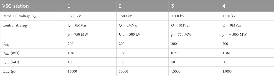
Table 1. Parameters of MMC-VSC

In order to accurately calculate the short circuit fault current, the four-terminal DC grid with three different types of CLCB shown in Figure 9A is established in EMT simulation tool PSCAD. The simulation results are illustrated in Figure 10 by the solid lines and its VSC in this DC grid model is based on the EMT equivalent model of half-bridge MMC proposed in (CIGRE WG B4.57, 2014; Gnanarathna et al., 2011). This simulation tool is generally considered to have the ability to accurately estimate the performance of an HVDC grid in normal or fault conditions, making the EMT simulation results a reliable reference criterion. In short circuit fault current calculation, getting the fault current curves is the most concerned. Therefore, Figure 10 shows solely the fault current i_1F and i_2F curves. However, EMT simulation would require a lot of computing resources and be expensive and time-consuming.

Figure 10

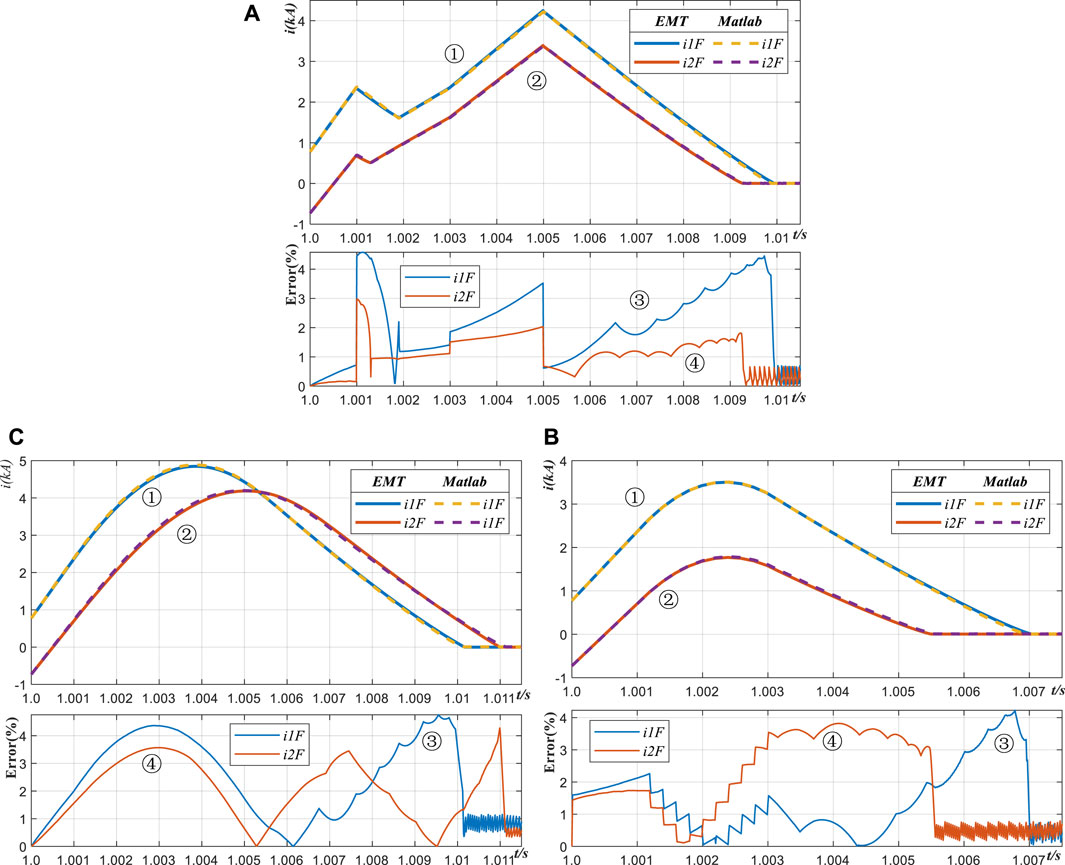
Figure 10. Fault current results of MTDC grid with different typical CLCB from EMT simulation and proposed fast-computing method; (A) MTDC grid with Inductance-CLCB (B) MTDC grid with MOA-CLCB (C) MTDC grid with Capacitance-CLCB.

In order to improve simulating efficiency, the short circuit fault current calculation equation is derived in Section 5 as expressed in Eq. 27. By applying the systematic formulation proposed in Section 2, the parameter matrices of the equivalent circuit shown in Figure 9B can be obtained. The incidence matrix A is also shown in Figure 2B, and Eq. 6 can be used to compute the P matrix. R and L matrices are

$\begin{array}{l}\mathbf{R}=\left[\begin{array}{lllll}{R}_1+R_{10}& 0& 0& 0& R_1\\ 0& R_2+R_{20}& R_2& 0& 0\\ 0& R_2& R_2+R_4+R_{24}& R_4& 0\\ 0& 0& R_4& R_3+R_4+R_{34}& -R_3\\ R_1& 0& 0& -R_3& R_1+R_3+R_{13}\end{array}\right]\\ \mathbf{L}=\left[\begin{array}{lllll}{L}_1+L_{10}& 0& 0& 0& L_1\\ 0& L_2+L_{20}& L_2& 0& 0\\ 0& L_2& L_2+L_4+L_{24}& L_4& 0\\ 0& 0& L_4& L_3+L_4+L_{34}& -L_3\\ L_1& 0& 0& -L_3& L_1+L_3+L_{13}\end{array}\right]\end{array}$

Using the MATLAB program to solve the short circuit fault current calculation equation set Eq. 27, we can obtain the fault current i_1F and i_2F curves illustrated in Figure 10 by the dotted lines. For the inductance-CLCB, the formula of Eq. 18 is utilized to express u_CLCBa and u_CLCBb in the voltage source rector of Eq. 27, and the simulation results are shown in Figure 10A. The Eq. 21 and Eq. 25 are used to express the voltage source rector of MOA-CLCB and capacitance-CLCB, respectively, and the simulation results are shown in Figures 10B,C, respectively.

Figure 10 shows four curves labelled ①, ②, ③ and ④. The curve ① and ② are the fault current i_1F and i_2F, respectively. It can be observed that the simulated results from MATLAB, indicated by the dotted lines, almost agreed with that of conventional EMT simulation shown in the solid lines. The curves ③ and ④ are error curves, illustrating that the maximum computing error is less than 5%. Therefore, these results confirm that the proposed model and formulas are accurate enough to can meet the requirement of routine engineering analysis and design.

In order to verify that the accuracy of the proposed DC fault current fast-computing method is not affected by changes in test conditions, such as the location of fault occurrence, we selected a four-terminal DC network with an inductive CLCB as the test object, as shown in Figure 9. Several rounds of the general EMT simulation and the proposed DC fault current fast-computing method were performed respectively on PSCAD and MATLAB under the same test conditions. However, the fault location was selected as a variable. The compared errors between the EMT simulating results and the proposed method calculating results are shown in Figure 11. In this case, the 2-D graph shown in Figure 10 becomes a 3-D graph in Figure 11.

Figure 11

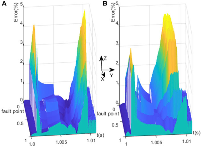
Figure 11. The Impact of fault location on the compared error of the proposed DC fault current fast-computing method: (A) fault current i1F (B) fault current i2F.

In these 3D graphs, the x-axis indicates the relative location of the short-circuit fault point, denoted as n_F, on the fault line. Let x be a ratio of L_fault/L_F-line, where L_fault represents the distance from the short circuit fault point n_F to VSC1, and L_F-line is the total length of the overhead line OL₁₂. The y-axis shows the time, and the vertical axes z shows the compared error between the proposed method and general EMT. Specifically, Figures 11A,B represent the errors fault current i_1F and i_2F, respectively. As shown in Figure 11, it can be observed that the maximum computing error is less than 5%, regardless of the location of the short circuit fault occurs on the line. Therefore, these results further confirm the accuracy of the proposed model and formulas with good stability and universality.

6.2 Computing efficiency

The simulation platform used in this paper was an AMD Ryzen7 4800H 2.90 GHz CPU with 16 GB of RAM and a 64-bit Windows 10 Operating System. The time step is 10 µs. For the PSCAD EMT simulation platform, it takes 0.9 s to start up. So, for the PSCAD EMT simulation and MATLAB calculation platform, let a dc short-circuit fault occurs at t = 1.0 s and fault time duration equals 10 ms. The time-consuming and efficiency improvements are listed in Table 2. It can be seen that the proposed short circuit current calculation method is much more efficient than the conventional EMT simulation and has relatively higher accuracy. The computing efficiency has been improved at least three hundred times, and the accuracy meets engineering analysis and design requirements.

Table 2

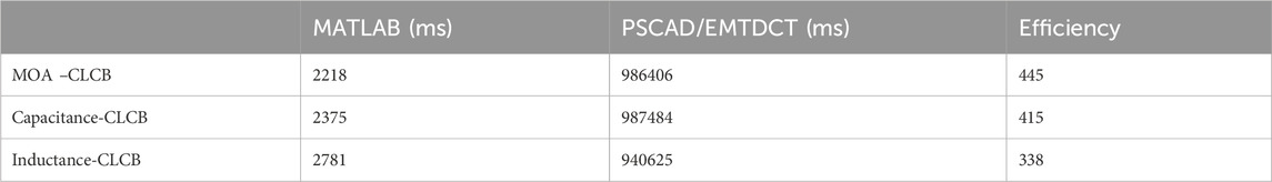
Table 2. Time-consuming and efficiency improving.

7 Performance comparison of three -typical CLCBs

Using the conventional EMT simulation tool would take a long time to estimate the performance of a DC grid with SCPE since it is a complex dynamic system. However, the proposed short circuit current calculation method offers greater computing efficiency and relatively higher accuracy. It is a powerful tool for one to analyses the performances of DC grid with SCPE. For DC grid projects that require the installation of SCPE equipment, this method can help design and quickly screen and evaluate the topology, configuration scheme and timing logic of the SCPEs.

To demonstrate this function, we analyze and compare the current limiting capabilities of three typical CLCBs under varying initial fault current values and fault locations and draw some significant conclusions. This will be done using the method described at the end of this paper.

7.1 Comparison of current limiting capability

At first, since ABB-DCCB is a typical hybrid DC circuit breaker and has been widely used in HVDC grids (Skarby and Steiger, 2013), it is applied to the four-terminal DC grid shown in Figure 9A. The EMT platform is utilized as a simulation tool to estimate its performance. The short circuit fault current simulation results are shown in Figure 12 by dotted lines, labelled as “i1F-DCCB” and “i2F-DCCB,” which is used as a reference criterion in this section.

Figure 12

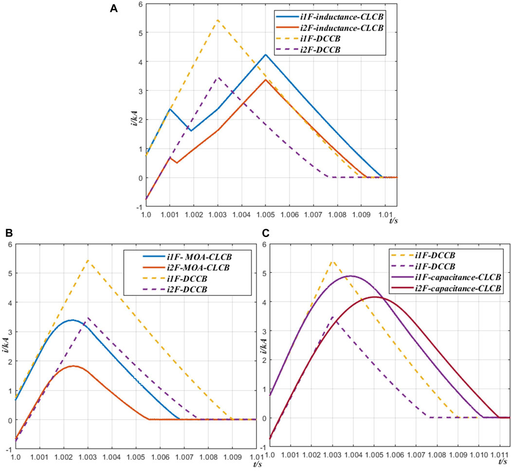
Figure 12. Comparison of current limiting capability of three CLCB (A) Inductance-CLCB (B) MOA-CLCB (C) Capacitance-CLCB.

In order to quickly compare the performance of the three typical CLCBs with the reference criterion, the proposed short circuit current calculation method is used to predict the fault currents. The simulation results are illustrated in Figures 12A–C by the solid lines, respectively.

According to Figure 12, it can be seen that the three typical CLCBs have a better fault current limiting ability than the conventional ABB-DCCB, and MOA-CLCB demonstrates the best performance. However, the other CLCBs take a longer fault isolation time than the conventional ABB-DCCB.

7.2 Impact of the normal current and fault location on CLCB performance

In the four-terminal DC network shown in Figure 9, the fault location n_F and normal current value are important parameters that will profoundly impact CLCB performance. Using the proposed short-circuit current calculation method, the performances of the three typical CLCBs can be estimated, and the simulation results are illustrated in Figure 13, which are three-dimensional graphs (3D graphs). The short-circuit fault current peak amplitude and fault isolation time of ABB-DCCB are also taken as standard values to evaluate the performance of the three typical CLCBs, such as peak fault current reduction value, peak current limiting ratio, and fault isolating time.

Figure 13

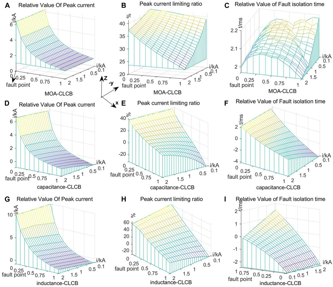
Figure 13. 3D performance graph of three typical CLCB; (A–C) The Impact of the normal current and fault location on the performance of MOA-CLCB. (D–F)The Impact of the normal current and fault location on the performance of capacitance-CLCB. (G–I) The Impact of the normal current and fault location on the performance of inductance-CLCB.

In these 3D graphs, the x-axis indicates the relative location of the short-circuit fault point n_F in the fault line. The y-axis shows the normal current, and the vertical axes z are the relative values of fault current peak amplitude, peak fault current limiting ratio and relative values of fault isolating time, respectively.

Figures 13A–C are the relative value of fault current peak amplitude, peak fault current limiting ratio and fault isolating time of the DC grid with MOA-CLCB, respectively. From Figure 13A, it can be observed that the relative value of the peak current amplitude depends on the fault point location and is almost independent of the normal value. However, the peak current limiting rate shown in Figure 13B is correlated with the fault point location and the normal value. As shown in Figure 13C, the isolating fault time of the MOA-CLCB is always shorter than that of ABB-DCCB. Consequently, MOA-CLCB demonstrates the best robustness performance among the three typical CLCBs.

Figures 13D–F demonstrate the performance of the capacitance-CLCB. The performance depends on both the short-circuit fault location and the normal value, but the short-circuit fault location has a more significant impact on the performance of capacitance-CLCB. When x > 0.8 and y < 0.5 kA, capacitance-CLCB will lose its current limiting ability.

Figures 13G–I show the performance of the inductance-CLCB, which is similar to that of the capacitance-CLCB. However, its current limiting effect is better than that of the capacitance-CLCB. It can be observed that there exists an optimal current limiting area, x < 0.3. In this area, the peak current limit rate exceeds 40%, and the relative value of peak current is greater than 5 kA. So, its current limiting effect is far better than the other two CLCBs in the optimal current limiting area. However, it is important to note that the inductance-CLCB achieves its best current limiting effect at the expense of a longer fault isolating time.

8 Conclusion

The proposed DC fault current fast-computing method is much more efficient than the conventional EMT simulation and has a relative higher accuracy. When compared to the conventional time-domain numerical DC fault current calculation method of MMC-HVDC grid, the proposed DC fault current fast-computing method offers three improvements.

Firstly, by applying modern electrical circuit theory, the proposed systematic formulation makes it easy to write the normal form of the differential equation set instead of writing the equation set using KVL, KCL, and VAR. This approach avoids complex and cumbersome manual matrix calculations, making the proposed calculation method suitable for handling large-scale MMC- HVDC grids.

Secondly, the proposed Y-Delta transformation in the s-domain can eliminate virtual nodes in short circuit fault RLC equivalent circuit of the complex MMC-HVDC grid. This progress makes the proposed calculation method suitable for handling complex structure MMC-HVDC grids.

Finally, to make SCPE become a linear circuit, a canonical voltage source model of SCPE is proposed. In this paper, three types of CLCB are taken as examples to introduce how to establish the canonical voltage source model of SCPE. This progress makes the proposed calculation method suitable for handling MMC-HVDC grids with SCPE and expands its application field.

To comparing with the conventional PSCAD/EMTDC, the computing efficiency is improved at least about three hundreds time and the accuracy can meet requirement of engineering analysis and design. In summary, the proposed method can be applied to large-scale MMC-HVDC grids with complex structures and provides a powerful tool for analysing fault currents and evaluating the performance of short-circuit protection devices.

It is first time in this paper to estimate and compare the performances of three typical CLCBs, obtaining some significant conclusions as the followings. 1). MOA-CLCB shows the best robustness performance in three typical CLCBs. 2). There is a lost current limiting area for capacitance-CLCB. 3). For the inductance-CLCB, there is an optimal current limiting area, in where its current limiting effect is far better than the other two CLCBs, but it is at expense of a longer fault isolating time.

Data availability statement

The original contributions presented in the study are included in the article/Supplementary material, further inquiries can be directed to the corresponding author.

Author contributions

XZ: Conceptualization, Data curation, Formal Analysis, Visualization, Writing–original draft, Writing–review and editing. XY: Project administration, Supervision, Writing–review and editing. CZ: Resources, Writing–review and editing, Investigation.

Funding

The author(s) declare that no financial support was received for the research, authorship, and/or publication of this article.

Conflict of interest

The authors declare that the research was conducted in the absence of any commercial or financial relationships that could be construed as a potential conflict of interest.

Publisher’s note

All claims expressed in this article are solely those of the authors and do not necessarily represent those of their affiliated organizations, or those of the publisher, the editors and the reviewers. Any product that may be evaluated in this article, or claim that may be made by its manufacturer, is not guaranteed or endorsed by the publisher.

Abbreviations

A, incidence matrix; C, capacitance; C_m, current limiting capacitance; D_m, freewheeling diode; i, current; i_c, capacitance current; i_Δ, current of Delta equivalent circuit; L, inductance; L_Δ, inductance of Delta equivalent circuit; MOA, metal-oxide arresters; n₀, fault point; R, resistance; R_∆, resistance of Delta equivalent circuit; T, IGBTs; Tm, IGBTs of current-limiting circuit; U_r, rated voltage of MOA; UFD, ultra-fast disconnectors; U_ref, reference voltage of MOA; u, voltage; u_moa, voltage of MOA; u_CLCB, voltage of CLCB; u_c, capacitance voltage; VSC, voltage-source converter.

References

Ahmad, M., Gong, C., Nadeem, M. H., Chen, H., and Wang, Z. (2022). A hybrid circuit breaker with fault current limiter circuit in a VSC-HVDC application. Prot. Control Mod. Power Syst. 7, 43. doi:10.1186/s41601-022-00264-9

CrossRef Full Text | Google Scholar

Alexander, C. K., and Sadiku, M. N. O. (2013). Fundamentals of electric circuits. New York, New York, United States: McGraw-Hill.

Google Scholar

An, T., Tang, G., and Wang, W. (2017). Research and application on multi-terminal and DC grids based on VSC-HVDC technology in China. High. Volt. 2, 1–10. doi:10.1049/hve.2017.0010

CrossRef Full Text | Google Scholar

Balabanian, N., and Bickart, T. A. (1969). Electrical network theory. Hoboken, New Jersey, United States: John Wiley & Sons.

Google Scholar

Belda, N. A., Plet, C. A., and Smeets, R. P. P. (2018). Analysis of faults in multiterminal HVDC grid for definition of test requirements of HVDC circuit breakers. IEEE Trans. Power Deliv. 33, 403–411. doi:10.1109/TPWRD.2017.2716369

CrossRef Full Text | Google Scholar

CIGRE WG B4.57 (2014). Guide for the development of models for hvdc converters in a hvdc grid. Available at: https://e-cigre.org/publication/604-guide-for-the-development-of-models-for-hvdc-converters-in-a-hvdc-grid (Accessed March 30, 2024).

Google Scholar

Gnanarathna, U. N., Gole, A. M., and Jayasinghe, R. P. (2011). Efficient modeling of modular multilevel HVDC converters (MMC) on electromagnetic transient simulation programs. IEEE Trans. Power Deliv. 26, 316–324. doi:10.1109/TPWRD.2010.2060737

CrossRef Full Text | Google Scholar

Hedayati, M., and Jovcic, D. (2017). Low voltage prototype design, fabrication and testing of ultra-fast disconnector (UFD) for hybrid DC CB. CIGRE Winn. 2017 Colloq.,

Google Scholar

Hedayati, M. H., and Jovcic, D. (2018). Reducing peak current and energy dissipation in hybrid HVDC CBs using disconnector voltage control. IEEE Trans. Power Deliv. 33, 2030–2038. doi:10.1109/TPWRD.2018.2812713

CrossRef Full Text | Google Scholar

Heidary, A., Bigdeli, M., and Rouzbehi, K. (2020). Controllable reactor based hybrid HVDC breaker. High. Volt. 5, 543–548. doi:10.1049/hve.2019.0354

CrossRef Full Text | Google Scholar

Li, B., Li, C., Li, B., Wen, W., Cui, H., and Su, J. (2021). Transient fault identification method for bipolar short-circuit fault on MMC-HVDC overhead lines based on hybrid HVDC breaker. High. Volt. 6, 881–893. doi:10.1049/hve2.12091

CrossRef Full Text | Google Scholar

Li, C., Zhao, C., Xu, J., Ji, Y., Zhang, F., and An, T. (2017b). A Pole-to-Pole short-circuit Fault Current calculation method for DC grids. IEEE Trans. Power Syst. 32, 4943–4953. doi:10.1109/TPWRS.2017.2682110

CrossRef Full Text | Google Scholar

Li, R., Xu, L., Holliday, D., Page, F., Finney, S. J., and Williams, B. W. (2016). Continuous operation of radial multiterminal HVDC systems under DC fault. IEEE Trans. Power Deliv. 31, 351–361. doi:10.1109/TPWRD.2015.2471089

CrossRef Full Text | Google Scholar

Li, T., Li, Y., Zhu, Y., Liu, N., and Chen, X. (2022). DC fault current approximation and fault clearing methods for hybrid LCC-VSC HVDC networks. Int. J. Electr. Power & Energy Syst. 143, 108467. doi:10.1016/j.ijepes.2022.108467

CrossRef Full Text | Google Scholar

Li, B., He, J., Tian, J., Feng, Y., and Dong, Y. (2017a). DC fault analysis for modular multilevel converter-based system. J. Mod. Power Syst. Clean Energy 5, 275–282. doi:10.1007/s40565-015-0174-3

CrossRef Full Text | Google Scholar

Martinez, J. A., and Durbak, D. W. (2005). Parameter determination for modeling systems transients—Part V: surge arresters IEEE PES task force on data for modeling system transients of IEEE PES working group on modeling and analysis of system transients using digital simulation (general systems subcommittee). IEEE Trans. Power Deliv. 20, 2073–2078. doi:10.1109/TPWRD.2005.848771

CrossRef Full Text | Google Scholar

Mohammadi, F., Rouzbehi, K., Hajian, M., Niayesh, K., Gharehpetian, G. B., Saad, H., et al. (2021). HVDC circuit breakers: a comprehensive review. IEEE Trans. Power Electron. 36, 13726–13739. doi:10.1109/TPEL.2021.3073895

CrossRef Full Text | Google Scholar

Ning, C., Xiang, C. U. I., Jiangjiang, M. A., and Lei, Q. I. (2019). Calculation method for line-to-ground short-circuit currents of VSC-HVDC grid. Electr. POWER Constr. 40, 119–127. doi:10.3969/j.issn.1000-7229.2019.04.014

CrossRef Full Text | Google Scholar

Saad, H., Peralta, J., Dennetière, S., Mahseredjian, J., Jatskevich, J., Martinez, J. A., et al. (2013). Dynamic averaged and simplified models for MMC-based HVDC transmission systems. IEEE Trans. Power Deliv. 28, 1723–1730. doi:10.1109/TPWRD.2013.2251912

CrossRef Full Text | Google Scholar

Safaei, A., Zolfaghari, M., Gilvanejad, M., and Gharehpetian, G. B. (2020). A survey on fault current limiters: development and technical aspects. Int. J. Electr. Power & Energy Syst. 118, 105729. doi:10.1016/j.ijepes.2019.105729

CrossRef Full Text | Google Scholar

Shu, H., Wang, S., and Lei, S. (2023). Single-ended protection method for hybrid HVDC transmission line based on transient voltage characteristic frequency band. Prot. Control Mod. Power Syst. 8, 26. doi:10.1186/s41601-023-00301-1

CrossRef Full Text | Google Scholar

Skarby, P., and Steiger, U. (2013). An ultra-fast disconnecting switch for a hybrid HVDC breaker—a technical breakthrough. Proc. CIGRÉ Sess., 1–9.

Google Scholar

Song, Y., Sun, J., Saeedifard, M., Ji, S., Zhu, L., Meliopoulos, A. P. S., et al. (2019). Reducing the fault-transient magnitudes in multiterminal HVdc grids by sequential tripping of hybrid circuit breaker modules. IEEE Trans. Industrial Electron. 66, 7290–7299. doi:10.1109/TIE.2018.2881941

CrossRef Full Text | Google Scholar

Stepanov, A., Mahseredjian, J., Karaagac, U., and Saad, H. (2021). Adaptive modular multilevel converter model for electromagnetic transient simulations. IEEE Trans. Power Deliv. 36, 803–813. doi:10.1109/TPWRD.2020.2993502

CrossRef Full Text | Google Scholar

Wang, W., He, Z., Li, G., Xin, Y., Gu, H., Zhu, L., et al. (2020). An inductively coupled HVDC current limiting circuit breaker. Proc. CSEE, 1731–1741. doi:10.13334/j.0258-8013.pcsee.190980

CrossRef Full Text | Google Scholar

Wu, Y., Peng, S., Wu, Y., Rong, M., and Yang, F. (2022). Technical assessment on self-charging mechanical HVDC circuit breaker. IEEE Trans. Industrial Electron. 69, 3622–3630. doi:10.1109/TIE.2021.3070523

CrossRef Full Text | Google Scholar

Wu, Y., Rong, M., Wu, Y., Yang, F., and Yi, Q. (2020). Damping HVDC circuit breaker with current commutation and limiting integrated. IEEE Trans. Industrial Electron. 67, 10433–10441. doi:10.1109/TIE.2019.2962475

CrossRef Full Text | Google Scholar

Xu, J., Zhu, S., Li, C., and Zhao, C. (2019). The enhanced DC Fault Current calculation method of MMC-HVDC grid with FCLs. IEEE J. Emerg. Sel. Top. Power Electron. 7, 1758–1767. doi:10.1109/JESTPE.2018.2888931

CrossRef Full Text | Google Scholar

Yang, X., Xue, Y., Wen, P., and Li, Z. (2018). Comprehensive understanding of DC pole-to-pole fault and its protection for modular multilevel converters. High. Volt. 3, 246–254. doi:10.1049/hve.2018.5045

CrossRef Full Text | Google Scholar

Ye, H., Gao, S., Li, G., and Liu, Y. (2021). Efficient estimation and characteristic analysis of short-circuit currents for MMC-MTDC grids. IEEE Trans. Industrial Electron. 68, 258–269. doi:10.1109/TIE.2020.2965433

CrossRef Full Text | Google Scholar

Zhang, S., Fan, Y., Lei, Q., Wang, J., Liu, Y., and Zhan, T. (2022). Insulation structure design and electric field simulation of 500 kV isolation energy supply transformer for HVDC breaker. High. Volt. 7, 185–196. doi:10.1049/hve2.12102

CrossRef Full Text | Google Scholar

Zhang, X., Zhuo, C., and Yang, X. (2023). A natural commutation current topology of hybrid HVDC circuit breaker integrated with limiting fault current. IET Generation, Transm. Distribution 17, 1509–1524. doi:10.1049/gtd2.12760

CrossRef Full Text | Google Scholar