The Blasingame method considering the effect of inter-well interference in a circular homogeneous closed reservoir

1 Introduction

In reservoirs with strong inter-well connectivity, neighbouring well interference can significantly impact test well pressures during the declining development process (Yuan and Wang, 2013; Guo et al., 2022; Wang et al., 2023). It has been well-established that reservoir dynamic description techniques, centred on single-well test well analysis and modern declining production analysis techniques, are effectively applied in reservoirs characterised by small single-well control ranges and poor inter-well connectivity (Zhang, 2004). However, reservoirs with high permeability and good connectivity are often multi-well systems (Zhang et al., 2006; Lin and Yang, 2007; Li and Luo, 2009). Therefore, interpreting such reservoirs using a single-well dynamic description can be misleading (Pang et al., 2012; Gan et al., 2022; Wang et al., 2023). Currently, the industry typically employs the superposition principle method to study the dynamic information of test wells in a multi-well system with inter-well interference (Onur et al., 1991; Li et al., 1994; Zhou et al., 2022). Jiaen Lin, Qiguo Liu, and Yonglu Jia demonstrated the late ‘upward curvature’ of the pressure recovery derivative curve in test wells by using the well test analysis technique (Dong and Zhai, 1996; Lin et al., 1996; Liu et al., 2002; Lin and Yang, 2005b; Liu et al., 2006; Jia et al., 2008; Deng et al., 2015). Hedong Sun provided a theoretical proof of this phenomenon while establishing an analysis method for multi-well pressure recovery test wells under neighbouring well interference conditions (Sun, 2016; Alarji. H et al., 2022). With the deepening of research, many scholars have explored the multi-well production model under the influence of multiple factors. Zeng Yang established a model for interpreting well tests in injection wells that consider interference from neighbouring wells (Zeng Y et al., 2020; Zhao et al., 2022). Cao established a well test interpretation model for finite inflow fractured wells under multi-well interference (Wei et al., 2022b).

The analytical solution of the multi-well production model discussed in previous studies is primarily used for analysing test wells (Jiang et al., 2019; Chen, 2023). The model assumes an infinite reservoir as the outer boundary condition, which simplifies the analysis. This paper introduces a closed reservoir as the outer boundary condition, introduces the ‘normalisation factor’, and applies the model’s solution to the Blasingame-type curves (Chen et al., 2017; Xu et al., 2021).

Modern methods of diminishing yield analysis and well test analysis are based on the classical seepage basis, but the two methods use different accuracy of evaluation data in the analysis process (Sun, 2013; Spivey, 2016; Wei et al., 2022a). Modern methods of diminishing yield analysis require less precision in the data and are, therefore, less difficult and costly to obtain. Blasingame and others creatively introduced the proposed time of material equilibrium and regularised yields to establish a plate of decreasing curves called the Blasingame plate (Mccray, T.L, 1990; Palacio and Blasingame, 1993). It is epoch-making in the modern analysis of diminishing yield.

2 Modelling and solving

Figure 1 shows a circular stratigraphic well deployment map.

Figure 1

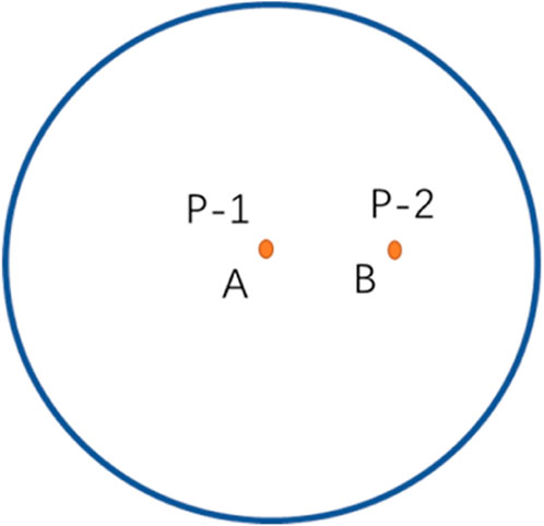
Figure 1. Circular stratigraphic well deployment map.

From Figure 1, the middle point of a circular formation with supply radius r_e and closed outer boundary, there is a well P-1 producing at a constant yield qi, while at point B, there is another well P-2 producing at a yield q₂, and the distance from point A to point B is L.

Other assumptions are as follows: the reservoir is homogeneous and isotropic, with impermeable boundaries above and below; the reservoir pores are filled with a single-phase, micro-compressible fluid, and the flow is in accordance with Darcy’s law; the effect of gravity is neglected; and the effects of the skin effect and the wellbore storage effect are not considered.

2.1 Equivalent well control radius

The pull-down spatial pressure solution for point A of the double-well production, Eq. 1, can be obtained according to the Duhamel superposition principle (Wang, 2015):

${\stackrel{\sim }{P}}_A={\stackrel{\sim }{P}}_{1A}+{\stackrel{\sim }{P}}_{2A},(1)$

where ${\stackrel{\sim }{P}}_A$ is the pressure solution at point A when both wells are producing, ${\stackrel{\sim }{\mathrm{P}}}_{1\mathrm{A}}$ is the pressure solution at point A when well P-1 is producing alone, and ${\stackrel{\sim }{P}}_{2A}$ is the pressure solution at point A when well P-2 is producing alone.

When L tends to 0, the pressure response of the unsteady seepage stage at point A is equivalent to the pressure response of well P-1 when it produces individually at a constant production rate $\left(q_i+q_2\right)$, and the unsteady flow stage exhibits radial flow characteristics. When L is large, $q_i=q_2$, and ${\stackrel{\sim }{P}}_{1A}$ > ${\stackrel{\sim }{P}}_{2A}$, the flow characteristics of the unstable seepage stage at point A are dominated by the flow characteristics of the unstable seepage stage at point A when well P-1 is producing alone.

Figure 2 shows a conceptual diagram of the r_eD2 solution. Overall, in Figure 2, the flow stage at point A, when the two wells are producing, can be simplified as the infinite radial flow stage, the proposed steady-state stage. In turn, the pressure solution at point A when well P-2 is producing alone can be simplified as the pressure solution for one well in the centre of a circular closed reservoir with constant production, while the simplified well control radius expression for well B is given in this paper.

Figure 2

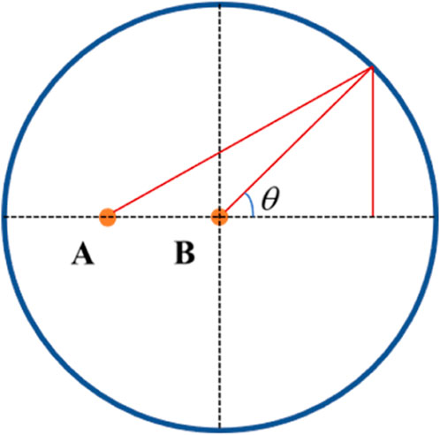
Figure 2. Conceptual diagram of the r_eD2 solution.

The average of the distances from point B to the circular closure boundary at the simplified drain radius is as follows:

${\mathit{r}}_{\mathit{e}\mathit{D}\mathbf{2}}=\frac{{\int }_{\mathbf{0}}^{\mathbf{2}\mathit{\pi }}\left[{\left({\mathit{r}}_{\mathit{e}\mathit{D}}\mathit{sin}\mathit{\theta }\right)}^{\mathbf{2}}+{\left({\mathit{r}}_{\mathit{e}\mathit{D}}\mathit{cos}\mathit{\theta }+{\mathit{r}}_{\mathbf{1}}\right)}^{\mathbf{2}}\right]\mathit{d}\mathit{\theta }}{\mathbf{2}\mathit{\pi }},(2)$

${\mathit{r}}_{\mathbf{1}}=\frac{\mathit{L}}{{\mathit{r}}_{\mathit{w}}},(3)$

${\mathit{r}}_{\mathit{e}\mathit{D}}=\frac{{\mathit{r}}_{\mathit{e}}}{{\mathit{r}}_{\mathit{w}}},(4)$

where $r_{eD}$ is the radius of the circular closed reservoir and $r_w$ is the radius of the wellbore.

From Eqs 2–4, we can derive $\left(r_{eD2}\ge r_{eD}\right)$ (take the equal sign when L = 0), so the reservoir reaches the proposed steady-state flow stage later when P-2 is producing alone than when well P-1 is producing alone, which is in line with the actual flow condition.

Table 1 lists the equivalent well control radius error rating table. After obtaining the simplified well control radius using this method, the corresponding equivalent well control area is further calculated and compared with the actual well control area. It is found that the simplified well control area is more accurate at $\left(r_1<0.5r_{eD}\right)$.

Table 1

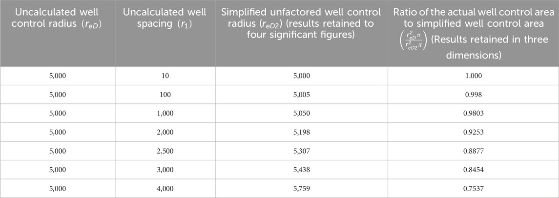
Table 1. Equivalent well control radius error rating table.

2.2 Modelling

The fixed solution problem for p-1 wells can be described as follows:

$\frac{{\partial }^{\mathbf{2}}{\mathit{p}}_{\mathit{D}}}{\partial {\mathit{r}}_{\mathit{D}}^{\mathbf{2}}}+\frac{\mathbf{1}}{{\mathit{r}}_{\mathit{D}}}\frac{\partial {\mathit{p}}_{\mathit{D}}}{\partial {\mathit{r}}_{\mathit{D}}}=\frac{\partial {\mathit{p}}_{\mathit{D}}}{\partial {\mathit{t}}_{\mathit{D}}},(5)$

${\left.p_D\right|}_{t_D=0}=0,(6)$

${\left.r_D\frac{\partial p_D}{\partial r_D}\right|}_{r_D=1}=-1,(7)$

${\left.\frac{{\partial p}_D}{\partial r_D}\right|}_{r_D=r_{eD}}=0,(8)$

$p_{1A}=p_D\left(1,t_D\right).(9)$

The fixed solution problem for p-2 wells can be described as follows:

$\frac{{\partial }^2{p}_D}{\partial r_D^2}+\frac{1}{r_D}\frac{\partial p_D}{\partial r_D}=\frac{\partial p_D}{\partial t_D},(10)$

${\left.p_D\right|}_{t_D=0}=0,(11)$

$q_B=\frac{q_2}{q_i},(12)$

${\left.r_D\frac{\partial p_D}{\partial r_D}\right|}_{r_D=1}=-q_B,(13)$

${\left.\frac{{\partial p}_D}{\partial r_D}\right|}_{r_D=r_{eD}}=0,(14)$

$p_{2A}=p_D\left(r_1,t_D\right).(15)$

The dimensionless variables are defined as follows:

$p_D\left(r_D,t_D\right)=\frac{kh}{1.842\times {10}^{-3}B{q}_i\mu }\left[p_i-p\left(r,t\right)\right],t_D=\frac{3.6kt}{\varnothing \mu C_t{r}_w^2},r_w=\frac{r}{r_w},r_{eD}=\frac{r_e}{r_w},r_{eD2}=\frac{{\int }_0^{2\pi }\left[{\left(r_{eD}\sin \theta \right)}^2+{\left(r_{eD}\cos \theta +r_1\right)}^2\right]d\theta }{2\pi },$

where $r$ is the distance from any point to the well in mm, $r_w$ is the wellbore radius in mm, $r_e$ is the drain radius in mm, $k$ is the reservoir permeability in µm², $\theta$ is the reservoir porosity with no causality, $C_t$ is the total reservoir compression factor in MPa⁻¹, $h$ is the thickness of the reservoir in mm, $\mu$ is the viscosity of the crude oil in MPa·s, B is a crude oil volume factor with no factorisation, q is the surface production of the well in m³/d, $p_i$ is the original stratigraphic pressure in MPa, $p$ is the formation pressure at a point in the reservoir at a given time in MPa, and $t$ is production time in h.

2.3 Solution of the mathematical model

A Laplace transformation of Eqs 5–15 yields

$\frac{{\partial }^2{\stackrel{\sim }{p}}_D}{\partial r_D^2}+\frac{1}{r_D}\frac{\partial {\stackrel{\sim }{p}}_D}{\partial r_D}=s{\stackrel{\sim }{p}}_D.(16)$

The boundary conditions within the P-1 well are expressed as

${\left.\frac{\partial {\stackrel{\sim }{p}}_D}{\partial r_D}\right|}_{r_D=1}=-\frac{1}{s}.(17)$

The boundary conditions within the P-2 well are expressed as

${\left.\frac{\partial {\stackrel{\sim }{p}}_D}{\partial r_D}\right|}_{r_D=1}=-\frac{q_B}{s},(18)$

${\left.\frac{\partial {\stackrel{\sim }{p}}_D}{\partial r_D}\right|}_{r_D=r_{eD}}=0.(19)$

Substituting Eq. 16 and Eq. 17 into Eq. 19, we have Eq. 20

${\stackrel{\sim }{p}}_{1A}=\frac{1}{s^{\frac{3}{2}}}\frac{K_0\left(\sqrt{s}\right)I_1\left(r_{eD}\sqrt{s}\right)+I_0\left(\sqrt{s}\right)K_1\left(r_{eD}\sqrt{s}\right)}{K_1\left(\sqrt{s}\right)I_1\left(r_{eD}\sqrt{s}\right)-I_1\left(\sqrt{s}\right)K_1\left(r_{eD}\sqrt{s}\right)}.(20)$

Substituting Eq.16 and Eq.18 into Eq. 19, we have Eq. 21

${\stackrel{\sim }{p}}_{2A}=\frac{q_B}{s^{\frac{3}{2}}}\frac{K_0\left(r_1\sqrt{s}\right)I_1\left(r_{e1D}\sqrt{s}\right)+I_0\left(r_1\sqrt{s}\right)K_1\left(r_{e1D}\sqrt{s}\right)}{K_1\left(\sqrt{s}\right)I_1\left(r_{e1D}\sqrt{s}\right)-I_1\left(\sqrt{s}\right)K_1\left(r_{e1D}\sqrt{s}\right)}.(21)$

Eq. 22 can be obtained from the Duhamel superposition principle:

${\stackrel{\sim }{p}}_A={\stackrel{\sim }{p}}_{1A}+{\stackrel{\sim }{p}}_{2A}.(22)$

3 Plotting Blasingame-type curves

Plots of the rate solution q_D under a constant BHFP and the reciprocal of the pressure solution at a constant rate (1/p_D) in the coordinate system are shown in Figure 3A. The figure indicates that the two curves almost overlap in the transient flow period and are dispersed in the boundary-dominated flow period. Palacio and Blasingame (1993) replaced dimensionless time t_D with dimensionless material balance time t_cD and plotted the above curves again. The result shows that the two curves overlap, as shown in Figure 3B. In other words, the solutions of variable flow rate and constant flow rate are equivalent due to the introduction of material balance time t_cD. Therefore, the Blasingame method is applicable to the condition of a variable BHFP and also to the condition of a variable flow rate (Liu, 2010; Yu, 2020).

Figure 3

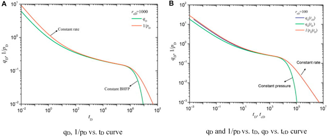
Figure 3. Comparison of fixed production pressure inverse, fixed production output, and fixed production material balance time output curves (A). q_D, 1/p_D vs. t_D curve; (B). q_D and 1/p_D vs. t_D, q_D vs. t_cD curve (Hedong Sun, 2015).

3.1 Blasingame-type curve definitions of the dimensionless parameters

Blasingame-type curve definitions of the dimensionless parameters are formed by introducing normalisation coefficients, $\alpha$, to the original definition of the dimensionless parameter.

Here, Blasingame-type curve definitions of the dimensionless parameters are as follows:

Define the dimensionless material balance time as Eq. 23

$t_{Dd}=\frac{1}{\frac{1}{2}\left(r_{eD}^2-1\right)\left(\mathit{ln}{r}_{eD}-\frac{1}{2}\right)}{t}_D.(23)$

Define the dimensionless decline flow rate Eq. 24

$q_{Dd}=\frac{\left(1+q_B\right)\left(\mathit{ln}{r}_{eD}-\frac{1}{2}\right)}{L^{-1}\left({\stackrel{\sim }{p}}_A\right)}.(24)$

Define the dimensionless cumulative production as Eq. 25

$N_{pDd}={\int }_0^{t_{Dd}}{q}_{Dd}\left(\tau \right)d\tau .(25)$

Define the dimensionless decline flow rate integral function as Eq. 26

$q_{Ddi}=\frac{{\int }_0^{t_{Dd}}{q}_{Dd}\left(\tau \right)d\tau }{t_{Dd}}=\frac{N_{pDd}}{t_{Dd}}.(26)$

Define the dimensionless decline flow rate integral derivative as Eq. 27

$q_{Ddid}=-\frac{d{q}_{Ddi}}{d\mathit{ln}{t}_{Dd}}=q_{Ddi}-q_{Dd}.(27)$

3.2 Blasingame-type curves and model validation

Figure 4 shows an unstable analysis curve of production from double straight wells in homogeneous reservoirs. From Figure 4, taking r_eD = 5,000 and q_B = 4 as an example, the crude oil flow can be roughly divided into an early radial flow stage, a stage influenced by the interference of neighbouring wells, and a later stage when the influence of the interfering wells is weakened (unsteady flow stage). The following section addresses the effect of well spacing, neighbouring well production, and neighbouring well start time factors on the Blasingame curve.

Figure 4

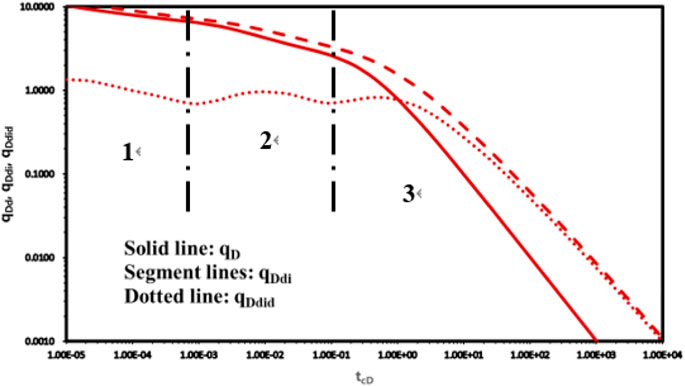
Figure 4. Unstable analysis curve of production from double straight wells in homogeneous reservoirs.

3.2.1 Effect of well spacing

Figure 5 shows the effect of different distances between two wells on the Blasingame curve when two wells in a circular homogeneous confined reservoir are producing at the same rate with simultaneous fixed production. From Figure 5, the early unstable flow stage of typical curves is a set of curves corresponding to different dimensionless well spacings, $r_1$. In the case of simultaneous production with the same yield, $r_1$ only affects the characteristics of the prior curve. When the pressure response from production from well P-2 has not yet reached point A, the curve is parallel to the curve when well p-1 is producing alone. When the pressure response from production in well P-2 reaches point A, inter-well interference occurs, and the regularised production curve begins to deviate downward. The larger the $r_1$, the greater the time for the material to begin to deviate from equilibrium, and the smaller the degree of $t_{Dd}$ deviation, eventually converging in the boundary control flow stage into a straight line with a slope of −1, which corresponds to the characteristics of the curve of the proposed steady-state flow of the p-1 well when it is producing alone at a constant production rate $2q_i$. The variation in the integral curve with the regularised yield is similar to that of the regularised yield curve, which is grouped into a single curve at a later stage. For the regularised yield integral derivative curves, the inter-well disturbances during the unsteady seepage phase make them convex, and the larger $r_1$ is, the later the convexity appears, the lower and narrower the convexity is, and the later it is reduced to a single curve.

Figure 5

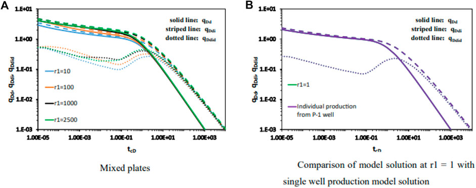
Figure 5. Effect of different distances between two wells on the Blasingame curve when two wells in a circular homogeneous confined reservoir are producing at the same rate with simultaneous fixed production (A) Mixed plates; (B) Comparison of model solution at r1=1 with single well production model solution.

Let $r_1$ be 1; the two wells overlap as one well on the model, and the Blasingame type-curves coincide exactly with that of the single-well model. The correctness of the above dimensionless pressure-fitting regularised yield solution is proved.

3.2.2 Effect of well spacing

Figure 6 shows the effect of Blasingame curves on P-2 delayed production from twin wells in circular homogeneous confined reservoirs producing at the same rate of constant production. Typical curves are a set of curves corresponding to the different dimensionless material balance time delays of P-2 wells (with fixed production rates, denoted as q_i) during the opening of the well. For the same production rate and constant well spacing, the larger is $t_p$, the greater the time for downward deviation of the regularised production curve, which eventually converges into a straight line with a slope of −1 at the boundary control flow stage, corresponding to the curve characteristic of the proposed steady-state flow of the P-1 well when it is producing alone at a constant production rate of $2q_i$. For the regularised yield integral curve, the variation with $t_p$ is similar to that of the regularised yield curve, but the larger $t_p$, the later the curve is shifted upward in parallel. For the regularised yield integral derivative curves, inter-well disturbances during the unsteady seepage phase make them convex, and the larger $t_p$ is, the later the convexity appears, the lower and narrower the convexity is, and the later curves are shifted upward in parallel.

Figure 6

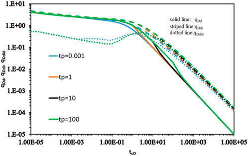
Figure 6. Effect of Blasingame curves on P-2 delayed production from twin wells in circular homogeneous confined reservoirs producing at the same rate of constant production.

3.2.3 Effect of production size of neighbouring wells

Figure 7 shows the effect of Blasingame curves in circular homogeneous closed reservoirs with two wells producing P-2 at different rates at the same time. Figure 7 shows that the type curves are a set of curves corresponding to the production of P-2 wells of different unfactored times. Under the condition of simultaneous production with the same well spacing, the larger $q_B$ is, the higher the regularised production curve is, the smaller the time of downward deviation is, the larger the degree of deviation is, and finally, a straight line with a slope of −1 converges at the stage of boundary control flow. For the regularised yield integral curve, the variation with $q_B$ is similar to that of the regularised yield curve, but the larger $q_B$, the later the curve is shifted downward in parallel. For the regularised production integral derivative curve, the inter-well interference during the unsteady seepage phase makes it convex, and the larger $q_B$ is, the faster the propagation of the pressure due to the production of the P-2 well is, the earlier the curve convexity appears, and the higher the convexity is.

Figure 7

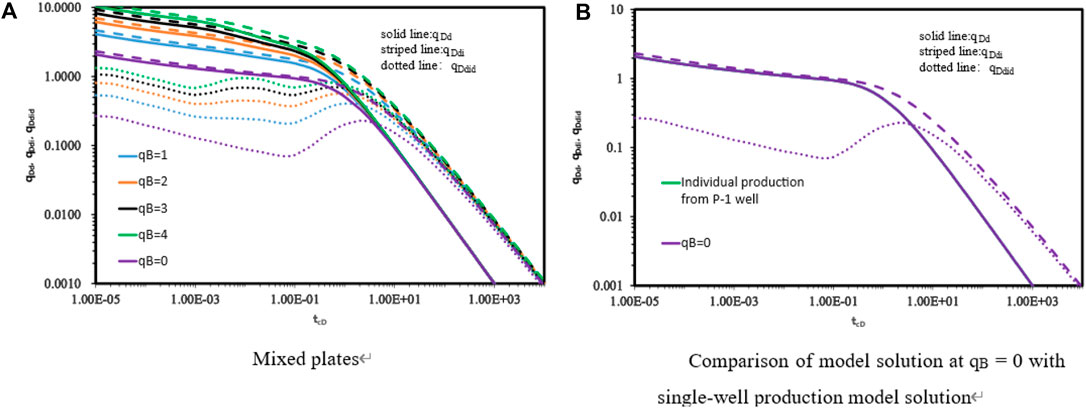
Figure 7. Effect of Blasingame curves in circular homogeneous closed reservoirs with two wells producing P-2 at different rates at the same time (A) Mixed plates; (B) Comparison of model solution at qB=0 with single well production model solution.

Let $q_B=0.$ Only well P-1 is producing in the model, and the Blasingame curve of its model solution coincides exactly with that of the single-well model, that is, the correctness of the above dimensionless fitted-pressure regularised production solution is proved again.

4 Comparative analysis of numerical simulations

Figures 8, 9 show the reservoir pressure map and plot of the bottomhole pressure, production, and cumulative production over time for the centre point wells.

Figure 8

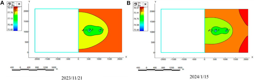
Figure 8. Reservoir pressure map (A) 2023/11/21; (B) 2024/1/15.

Figure 9

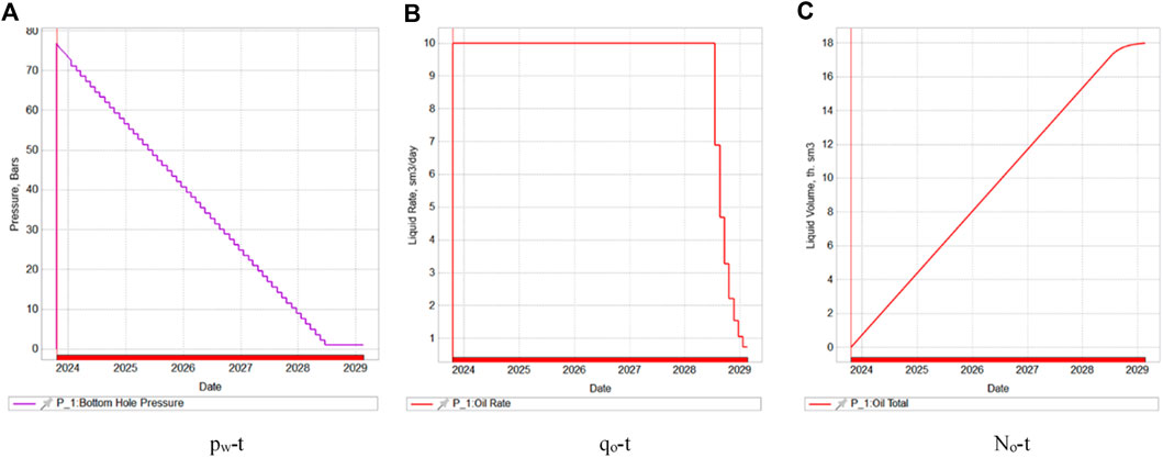
Figure 9. Plot of bottomhole pressure, production, and cumulative production over time for centre-point wells (A). p_w-t; (B). q_o-t; (C). N_o-t.

From Figures 8, 9, tNavigator software was used to establish a 2000 m × 2000 m × 20 m reservoir 3-D model, with a grid step of 5 m, net-to-gross ratio of 0.1, porosity of 0.1, X-axis permeability of 100 mD, X-axis permeability of 100 mD, Z-axis permeability of 10 mD, an initial pressure of 80 MPa, a support depth of 110 m, a single-component model, a well at the centre point producing at a fixed rate, and another well at the grid coordinates (100, 100, 1) producing at the same rate, and two wells producing at the same time, and obtaining the data on the bottomhole pressure, the production rate, and the cumulative production rate of the wells at the centre point with the change of time.

4.1 Data processing

To regularise the resultant data from numerical model runs,

Calculate the material balance time by Eq. 28

$t_c=\frac{N_p}{q}.(28)$

Calculate the normalised rate by Eq. 29

$\frac{q}{∆p}=\frac{q}{p_i-p_{wf}}.(29)$

Calculate the normalised rate integral by Eq. 30

${\left(\frac{q}{∆p}\right)}_i=\frac{1}{t_c}{\int }_0^{t_c}\frac{q}{p_i-p_{wf}}dx.(30)$

Calculate the normalised rate integral derivative by Eq. 31

${\left(\frac{q}{∆p}\right)}_{id}=-t_c\frac{d{\left(\frac{q}{∆p}\right)}_i}{d{t}_c}.(31)$

Table 2 is the numerical simulation data–production data regularisation table.

Table 2

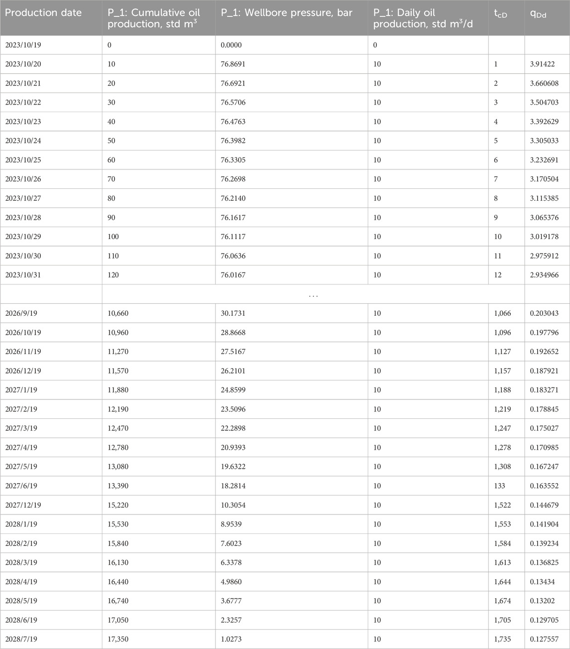
Table 2. Numerical simulation data–production data regularisation table.

4.2 Data fitting

Figure 10 shows measured curve fitting results from plotting the three relational curves, q_d-t_c, q_di-t_c, and q_did-t_c, fitting the Blasingame yield instability analysis plate, and recording the fitted values, where the three relational curves can be used simultaneously or individually.

Figure 10

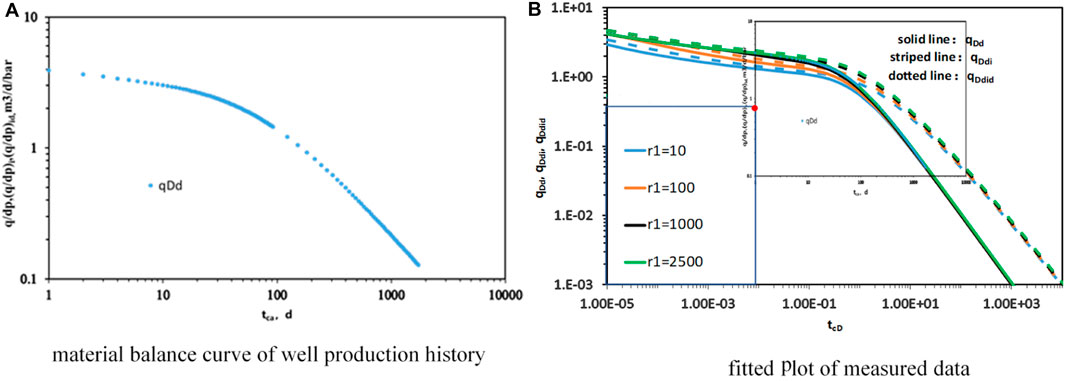
Figure 10. Measured curve fitting results (A) material balance curve of well production history; (B) fitted plot of measured data.

Using the theoretical fit points (8 × 10⁻³, 0.4), the actual fit points can be obtained (1, 0.7).

The dynamic reserve at the centre point can be calculated according to the following Eq 32:

$N=\frac{1}{C_t}{\left(\frac{t_c}{t_{Dd}}\right)}_M{\left(\frac{q/∆p}{q_{Dd}}\right)}_M\left(1-S_w\right)(32)$

as $3.65\times {10}^6$ m³, and the numerical model has a reserve of $7.68\times {10}^6$ m³.

Additionally, the flowing material balance method (FMB) is listed for comparison to verify the accuracy of the method used in this article.

Figure 11 shows the equilibrium curves for the flowing material balance.

Figure 11

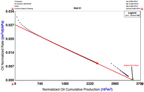
Figure 11. Fluid substance balance analysis diagram.

FMB is a method similar to the traditional material balance equation. However, it differs from the traditional material balance equation in that it uses dynamic pressure data instead of static pressure data for storage evaluation. Additionally, it differs from the flow material balance method, which uses flow pressure for dynamic storage evaluation. Once the reservoir is producing and has achieved a steady-state flow, the following relationship can be established (Eq. 33):

$\frac{q}{∆p}=-\frac{N_p}{b_{pss}N∆p{C}_t}+\frac{1}{b_{pss}}.(33)$

The dynamic reserves N can be determined from the intercept results if the $\frac{q}{∆p}—\frac{N_p}{∆p{C}_t}$ curve is plotted.

From Figure 11, the dynamic reserves calculated for the P-1 well’s reservoir are $3.486\times {10}^6$ m³. Comparing the results of the two methods, it is found that the method in this paper is more accurate in its calculations.

5 Conclusion

In this paper, the dual-well model is solved analytically by the equivalent well control radius method, and the following conclusions are reached:

(1) Based on establishing a constant production model that takes into account the effect of the presence of inter-well interference, the method of equivalent well control radius is used to simplify the treatment of the external boundary conditions of neighbouring wells that are not at the centre point of a circular closed reservoir. The range of applicability of the method is verified by comparing the equivalent well control surface with the actual well control area, and it is found that the method is more accurate when $\left(r_1<0.5r_{eD}\right)$.

(2) Based on the method of equivalent well control radius, a sensitivity analysis of the Blasingame curve for the dual-well model can be conducted with respect to the parameters of adjacent well production, well spacing, and adjacent well opening time: the Blasingame normalised dimensionless decline flow rate integral curve is shifted downward when inter-well interference occurs, returning to a straight line later in the season. The Blasingame normalised dimensionless decline flow rate integral curve is shifted downward in the early stage, and the shape of the curve in the later stage is determined by the parameters. The Blasingame normalised dimensionless decline flow rate integral derivative curve has convex bulges, and the higher the degree of interference between the wells, the higher the bulges are, and the earlier they appear.

(3) Using the double-well production Blasingame curve plate for decreasing production analysis, the interpreted dynamic reserve results are more accurate for reservoirs with inter-well interferences, and the method in this paper can provide technical support for the fine evaluation of such reservoirs.

(4) Shortcomings: At present, the method is only applicable to analytical solutions and is used under the condition that r₁ (distance between wells) > r_eD (actual well control radius). This is somewhat inapplicable to more complex models, such as composite media models, and requires further investigation.

Data availability statement

The original contributions presented in the study are included in the article/supplementary materials; further inquiries can be directed to the corresponding author.

Author contributions

PD: writing–original draft. QW: writing–review and editing. JZ: writing–review and editing. YW: writing–review and editing. DW: supervision and writing–review and editing. YH: software, supervision, and writing–review and editing. PL: validation and writing–review and editing.

Funding

The author(s) declare financial support was received for the research, authorship, and/or publication of this article from The National Natural Science Foundation of China (Grant No. 52074344).

Conflict of interest

The authors declare that the research was conducted in the absence of any commercial or financial relationships that could be construed as a potential conflict of interest.

Publisher’s note

All claims expressed in this article are solely those of the authors and do not necessarily represent those of their affiliated organizations, or those of the publisher, the editors, and the reviewers. Any product that may be evaluated in this article, or claim that may be made by its manufacturer, is not guaranteed or endorsed by the publisher.

References

Alarji, H., Clark, S., and Regenauer-Lieb, K. (2022). Wormholes effect in carbonate acid enhanced oil recovery methods. Adv. Geo-Energy Res. 6 (6), 492–501. doi:10.46690/ager.2022.06.06

CrossRef Full Text | Google Scholar

Chen, M., Wang, Z., Sun, H., Chang, C., Fuller, P. M., and Lu, J. (2017). Ventral medullary control of rapid eye movement sleep and atonia. Petroleum Sci. Bull. 2 (1), 53–62. doi:10.1016/j.expneurol.2017.01.002

PubMed Abstract | CrossRef Full Text | Google Scholar

Chen, Y. Q., Wang, X., and Liu, Y. (2023). The problems and derivation of Blasingame's steady-state pressure drop equation for variable production wells and its application. J. China Offshore Oil Gas 35 (6), 70–77. doi:10.2118/JCM-2023-35-6-070

CrossRef Full Text | Google Scholar

Deng, Q., Nie, R., Jia, Y., Wang, X., Chen, Y., and Xiong, Y. (2015). “A new method of pressure buildup analysis for a well in a multi-well reservoir,” in SPE North Africa Technical Conference and Exhibition, Cairo, Egypt, September 14-16, 2015.

CrossRef Full Text | Google Scholar

Dong, J., and Zhai, Y. (1996). “Study on theoretical curve of well test under multi-well interference conditions,” in Proceedings of the 5th National Symposium on Seepage Hydraulics SPE Asia Pacific Improved Oil Recovery Conference, Kuala Lumpur, Malaysia, October 25-26, 1999 (Beijing: Petroleum Industry Press), 188–193.

Google Scholar

Gan, X., Yi, J., Ou, J., Yuan, Q., Deng, Z., Yan, P., et al. (2022). Numerical well test technology of gas well pressure recovery based on inter-well interference model. Well Test. Oil Gas Wells 31 (3), 9–15. doi:10.19680/j.cnki.1004-4388.2022.03.002

CrossRef Full Text | Google Scholar

Guo, J., Ning, B., Yan, H., Jia, C., and Li, Y. (2022). Production performance analysis for deviated wells in carbonate gas reservoirs with multiple heterogeneous layers. Front. Energy Res. 10. doi:10.3389/fenrg.2022.861780

CrossRef Full Text | Google Scholar

Jiang, R. Z., He, J. X., and Jiang Yu, F. H. (2019). Establishment and application of Blasingame's production decline analysis method for fractured horizontal wells in shale gas reservoirs. Acta Pet. Sin. 40 (12), 1503–1510. doi:10.7623/syxb201912009

CrossRef Full Text | Google Scholar

Li, X., and Luo, J. (2009). Application research on the well test analysis model under the influence of adjacent wells. Well Test. 18 (2), 5–7. doi:10.3969/j.issn.1004-4388.2009.02.002

CrossRef Full Text | Google Scholar

Lin, J., Liu, W., and Chen, Q. (1996). Application of the analysis theory of multi-well system for water injection development. Petroleum Explor. Dev. 23 (3), 58–63.

Google Scholar

Lin, J., and Yang, H. (2005b). Pressure buildup analysis for a well in a closed, bounded multi-well reservoir. Chin. J. Chem. Eng. 13 (4), 441–450. doi:10.1002/cite.200590223

CrossRef Full Text | Google Scholar

Lin, J., and Yang, H. (2007). “Analysis of well-test data in a multi-well reservoir with water injection,” in SPE Annual Technical Conference and Exhibition, Anaheim, California, November 11-14, 2007.

Google Scholar

Liu, Q., Chen, Y., Zhang, L., and Wang, W. (2006). Study on the model and interpretation method of interference well testing without shutting in. Well Test. 15 (1), 10–12. doi:10.3969/j.issn.1004-4388.2006.01.004

CrossRef Full Text | Google Scholar

Liu, X., Zou, C., Jiang, Y., and Yang, X. (2010). Basic principles and applications of modern production decline analysis. Nat. Gas. Ind. 30 (5), 50–54. doi:10.3787/j.issn.1000-0976.2010.05.012

CrossRef Full Text | Google Scholar

Liu, Y., Chen, H., Zhang, D., Zhou, R., and Liu, Y. (2002). Numerical well test analysis of oil wells under the condition of adjacent well influence. Well Test. 11 (5), 4–7. doi:10.3969/j.issn.1004-4388.2002.05.002

CrossRef Full Text | Google Scholar

Liu, Y., Jia, Y., Kang, Y., and Huo, J. (2008). A survey of genetic simulation software for population and epidemiological studies. Drill. Prod. Technol. 31 (1), 79–86. doi:10.1186/1479-7364-3-1-79

PubMed Abstract | CrossRef Full Text | Google Scholar

Li, S., Zhou, R., and Huang, B. (1994). Theoretical analysis and application of interference pressure among adjacent wells. Petroleum Explor. Dev. 1 (1), 84–88. 128.

Google Scholar

Mccray, T. L. (1990). Reservoir analysis using production decline data and adjusted time. United States: Texas A&M University.

Google Scholar

Onur, M., Serra, K. V., and Reynolds, A. C. (1991). Analysis of pressure buildup data from a well in a multi-well system. SPE Form. Eval. 6 (1), 101–110. doi:10.2118/18123-pa

CrossRef Full Text | Google Scholar

Palacio, J. C., and Blasingame, T. A. (1993). Decline-curve analysis using type curves analysis of gas well production data. SPE 25909.

Google Scholar

Pang, J., Lei, G., Liu, H., and Zhang, X. (2012). Evaluation of well-to-well interference in gas wells using the material balance method. Sci. Technol. Eng. 12 (26), 6787–6789. 6793. doi:10.3969/j.issn.1671-1815.2012.26.049

CrossRef Full Text | Google Scholar

Spivey, J. P., and John Lee, W. (2016). Practical well test interpretation methods, translated by yongxin han, H Sun, xg Deng, and Y shi. Beijing: Petroleum Industry Press.

Google Scholar

Sun, H. (2005). Advanced production decline analysis and application. Oxford: Gulf Professional Publishing.

Google Scholar

Sun, H. (2013). Modern production decline analysis method and application of oil and gas wells. Beijing: Petroleum Industry Press.

Google Scholar

Sun, H. (2015). Advanced production decline analysis and application. Gulf Professional Publishing.

Google Scholar

Sun, H. (2016). Analysis method of multi-well pressure recovery well test under the condition of adjacent well interference. Nat. Gas. Ind. 36 (5), 62–68. doi:10.3787/j.issn.1000-0976.2016.05.009

CrossRef Full Text | Google Scholar

Wang, F. (2015). Diagnosis of nonlinear reservoir behaviour for correctly applying the superposition principle and deconvolution. J. Nat. Gas Sci. Eng. 26, 630–641. doi:10.1016/j.jngse.2015.07.004

CrossRef Full Text | Google Scholar

Wang, Y., Dai, Z., Chen, Li, Shen, X., Chen, F., and Soltanian, M. R. (2023). An integrated multi-scale model for CO2 transport and storage in shale reservoirs. Appl. Energy 331, 120444. doi:10.1016/j.apenergy.2022.120444

CrossRef Full Text | Google Scholar

Wang, Y.-W., and Dai, Z.-X. (2023). A hybrid physics-informed data-driven neural network for CO2 storage in depleted shale reservoirs. Petroleum Sci. 16 (1), 109–120. doi:10.3969/j.issn.1000-9585.2023.01.014

CrossRef Full Text | Google Scholar

Wei, C., Cheng, S., Bai, J., Li, Z., Shi, W., Wu, J., et al. (2022b). Analytical well test analysis method for finite conductivity fractured well under multi-well interference. Petroleum Geol. Oilfield Dev. Daqing 41 (4). doi:10.19597/J.ISSN.1000-3754.202103018

CrossRef Full Text | Google Scholar

Wei, C., Cheng, S., Jiang, B., Li, Z., Shi, W., Wu, J., et al. (2022a). Analytical well test analysis method for finite conductivity fractured wells under multi-well interference. Daqing Petroleum Geol. Dev. 41 (4), 90–97. doi:10.19597/J.ISSN.1000-3754.202103018

CrossRef Full Text | Google Scholar

Xu, Y., Liu, Q., Xiaoping, Li, Wang, X. J., Liang, H. S., Zeng, Z. C., et al. (2021). Fbf1 regulates mouse oocyte meiosis by influencing Plk1. Nat. Gas. Ind. 41 (6), 74–83. doi:10.1016/j.theriogenology.2021.01.018

CrossRef Full Text | Google Scholar

Yu, Q., Hu, X., Li, Y., and Jia, Y (2020). Dynamic evaluation method of oil well parameters and reservoir parameters in drilling large caves. Oil Gas Geol. 41 (3), 647–654. doi:10.11743/ogg20200320

CrossRef Full Text | Google Scholar

Zeng, T., Jia, Y., Wang, H., Tang, D., and Zhang, W. (2006). Analysis of the finite multi-well system well test model and template curve. Xinjiang Pet. Geol. 27 (1), 86–88. doi:10.3969/j.issn.1001-3873.2006.01.024

CrossRef Full Text | Google Scholar

Zeng, Y., Kang, X., Tang, E., Liang, D., and Cheng, S. (2020). A new well test interpretation model for injection polymer wells considering adjacent well interference. J. Chengdu Univ. Technol. Sci. Technol. Ed. 47 (1), 85–91. doi:10.3969/j.issn.1671-9727.2020.01.08

CrossRef Full Text | Google Scholar

Zhang, L., Xiang, Z., Li, Y., Li, X., and Liu, Q. (2006). Impact of well-to-well interference on oil-water two-phase flow numerical well test curves. J. Hydrodynamics Ser. A 21 (6), 805–810.

Google Scholar

Zhang, X., Jia, Y., Yan, T., Peng, H., Wergedal, J. E., Guttierez, G. G., et al. (2004). Local ex vivo gene therapy with bone marrow stromal cells expressing human BMP4 promotes endosteal bone formation in mice. Well Test. Technol. 25 (3), 4–15. doi:10.1002/jgm.477

PubMed Abstract | CrossRef Full Text | Google Scholar

Zhao, J., Wang, L., Liu, S., Kang, Z., Yang, D., and Zhao, Y. (2022). Numerical simulation and thermo-hydro-mechanical coupling model of in situ mining of low-mature organic-rich shale by convection heating. Adv. Geo-Energy Res. 6 (6), 502–514. doi:10.46690/ager.2022.06.07

CrossRef Full Text | Google Scholar

Zhou, S., Wang, H., Li, B., Li, S., Sepehrnoori, K., and Cai, J. (2022). Predicting adsorbed gas capacity of deep shales under high temperature and pressure: experiments and modeling. Adv. Geo-Energy Res. 6 (6), 482–491. doi:10.46690/ager.2022.06.05

CrossRef Full Text | Google Scholar