Forecasting of energy efficiency in buildings using multilayer perceptron regressor with waterwheel plant algorithm hyperparameter

1 Introduction

Climate change has severe effects on all living organisms on Earth. Global warming is a phenomenon within climate change that involves an increase in the average temperature of the Earth’s surface (Rodríguez et al., 2020). Higher electricity usage is a significant contributor to the release of greenhouse gases, leading to global warming (Mastrucci et al., 2021). Carbon dioxide (CO₂) is the primary greenhouse gas that significantly contributes to global warming, and its emissions have been steadily rising over the years (Yoro and Daramola, 2020). In 2019, worldwide CO₂ emissions were 45% greater than the emissions between 1980 and 1990 and doubling the amount of CO₂ would result in a 3.8°C increase in global temperatures (Al-Ghussain, 2019). The energy usage of the building sector is one of the major ones among the three sectors: transportation, industry, and construction (Prasetiyo et al., 2019). As per the International Energy Agency (IEA), buildings consume 40% of the total energy and 24% of the global CO2 emission (Zhang et al., 2023). Building, industry, and transportation represent 41%, 30%, and 29%, respectively, of the energy demand in the USA (Chou and Bui, 2014). Thus, the reduction of building energy consumption is crucial.

The US Department of Energy reported that 40% of greenhouse gas emissions coming from residential and commercial buildings would be cut by 2010 (Ahmad and Zhang, 2020). Commercial buildings utilized more than 60 percent of electricity in 2016 (Lokhandwala and Nateghi, 2018). Commercial building cooling energy usage influences factors that need to be comprehended for sustainability and environmental impact reduction. Among those are heating, ventilation, and air conditioning (HVAC), population growth, dwell duration, and climate (Invidiata et al., 2018). Other variables that influence building energy use cover weather conditions, dry bulb temperature, material properties and floor count (Araújo et al., 2023). Besides, building characteristics have a marked influence on energy consumption, and effective design practices can reduce energy demand (Tsanas and Xifara, 2012). It is also important to know how building architecture influences energy efficiency; bad design and structure would cause about 40% more CO₂ emissions from energy usage (Xu et al., 2012). It is advisable to analyze building energy implementation in heating load (HL) and cooling load (CL). Building energy use is affected by climate location (Renuka et al., 2022). Various climates are hot, cold, moist and arid conditions (Phan and Lin, 2014). As a result, building energy requirements change with local climatic conditions. Machine learning for analysis is a quick and easy approach since it uses algorithms to both predict and classify a given training dataset (Xie et al., 2022). Models of machine learning are known for their aptitude to recognize trends and patterns. It can analyze large and complex data and detect patterns that humans find hard to process manually. Further, ML can work with multi-dimensional data in dynamic situations (Dahiya et al., 2022). They applied ML to find energy-related data patterns, which made it popular in many fields, including healthcare. Supervised machine learning uses a labeled dataset for predictions (Wang et al., 2021). Test conditions for the models include train-test split and k-fold cross validation. K-fold cross validation is a reliable method that involves partitioning data into k subsets or folds, with each fold serving as test data and others as training data (Chou and Bui, 2014).

This paper proposes an automated hyperparameter optimization technique using WWPA and MLPRegressor to forecast the cooling/heating loads in a building. Through an analysis of factors influencing heating and cooling energy usage, this paper aims to enhance the energy efficiency of residential and commercial buildings.

The following is an outline of the structure of this article: In the second section, a detailed overview of the available literature on the application of machine learning algorithms in energy efficiency in buildings is presented. In the third section, the model that was proposed in this study is presented. Section 4 provides a comprehensive review of the performance of the machine learning methods and materials that were utilized. The paper is concluded in Section 5, which also provides some suggestions for potential future research.

2 Literature review

The rise in the average surface temperature, sometimes known as global warming, is a huge problem all around the globe that humans are making worse (Al-Ghussain, 2019). The problem is not limited to humans; it impacts all forms of life. The main source of global warming is the emission of greenhouse gases, which include water vapour, methane, carbon dioxide, and nitrous oxide. Carbon dioxide accounts for 76% of all emissions of greenhouse gases, making it the most important of these gases. According to (Chou and Bui, 2014), about 41% of the United States’ energy consumption is attributable to buildings, both residential and commercial. Design characteristics, population density, and urbanization are some of the elements that influence buildings’ energy usage (Aqlan et al., 2014).

The recent rise in building energy consumption is a result of factors including climate change, demand for building services, population, and building characteristics (Kim and Suh, 2021; Zhang et al., 2023) point out the necessity of the design of architectural parameters as a route to minimizing energy use in buildings. This can be achieved by adjustment and improvement of these design aspects. One of the major components that influences energy consumption is building design (Chung and Rhee, 2014). Location is another aspect that affects the energy use of a structure due to the weather and temperature conditions of its location. One of the approaches to increasing the energy efficiency of a building is to adapt its design to the individual location (Ascione et al., 2019). Recognizing which factors are most critical in defining a building’s energy consumption is vital. To focus their works and investments on energy efficiency, architects need to find the most significant features or components affecting the building’s energy consumption (Medal et al., 2021).

The basic factors that characterize the environment include the heating and cooling loads, which are the amount of energy that needs to be added within the building or removed from it per unit of time (Shanthi and Srihari, 2018). Determining the HL and CL of a building is crucial in understanding how much equipment is required to maintain the temperature inside at an optimal level, which is beneficial in terms of cost and environmental factors (Abediniangerabi et al., 2022). Researchers have used the UCI energy efficiency dataset to look at how much energy a building uses by looking at eight design variables: the height of the building, orientation, surface area, wall area, roof area, and the Distribution of its glazing area. The output variables in the UCI dataset include heat load and cool load. Most of these input factors have been employed in a number of studies for the prediction of heating and cooling loads (Aqlan et al., 2014). discovered that the main parameters influencing HL and CL are RC, wall area, surface area, roof area, total height and glazing area. They found that, in general, the height of a building has a major influence on the energy it uses for heating and cooling. The research carried out by (Tsanas and Xifara’s, 2012) on the HL and CL factors found that the effect of these coefficients on energy loads was greater for RC, Wall area and Roof area than for any other variables. The research done by (Irfan and Ramlie, 2021) investigated the effect of input factors on two output variables, HL and CL. According to their findings, orientation does not have much impact on the change of HL and CL.

(Lops, C., et al., 2023; Caroprese, L., et al., 2024) use deep learning framework (DLF) to enhance precision of fifth-Generation Mesoscale Model (MM5) weather variable predictions through sophisticated architecture through around gated recurrent unit neural networks. The DLF improves the accuracy of MM5 forecasts, leading to enhanced precision in predictions. The effectiveness of the model is evaluated using statistical metrics such as mean absolute error which provide insights into its performance.

The fundamental factors that define the environment are heating and cooling loads, which indicate how much energy needs to be added or removed from the building per unit of time (Shanthi and Srihari, 2018). Determination of the HL and CL of a building helps to determine the kind of equipment that is required to maintain the temperature within the building, which is also cost-effective and environmentally friendly (Abediniangerabi et al., 2022). Researchers have used the UCI energy efficiency dataset to look at how much energy a building uses by looking at eight design variables: the total height of the building, the orientation, the surface area, the wall area, the roof area, and the glazing area distribution of it. Heat and cool loads are the two outputs in the UCI dataset. Several studies have employed these input factors to forecast the heating and cooling loads. The most crucial factors determining HL and CL, according to Aqlan et al. (2014), were RC, wall area, surface area, roof area, total height and glazing area. They concluded that the overall height of the building has a significant impact on the amount of energy that it requires for heating and cooling. The research of Tsanas and Xifara (2012) on the factors of HL and CL determined that RC, wall area, and roof area have the greatest impact on energy loads as compared to other variables. Orientations did not show a significant effect on the changes of both HL and CL, as demonstrated by the research of (Irfan and Ramlie, 2021). The general height, wall area, and surface area do, however, have a big effect on both energy loads. That study by (Nazir et al., 2020) found that RC, total height, wall area, glazing area, surface area, and roof area are the most important things that affect predicting heating and cooling loads. The study did not look into whether independent factors had positive or negative effects or whether there were linear relationships between them and dependent variables.

A key component of artificial intelligence is the ability to teach computers to mimic human intelligence and do tasks once performed only by humans, such as learning, reasoning, and decision-making (Eid M., et al., 2022; Khafaga, 2022; Samee, et al., 2022). Image processing and intelligent robots are just two of the many uses for artificial intelligence (van der Velden et al., 2022). XAI is a technique that is used to make machine learning models more explainable. XAI (Machlev et al., 2022) aims to improve the understanding of ML outputs. The use of XAI methods is applied to comprehend better how input variables influence output (Tsoka et al., 2022). XAI also provides clarity about the way AI models make decisions, which increases trust in those models (Ersoz et al., 2022). XAI offers a high-performance and precise method for researchers to study the performance of the ML models (Machlev et al., 2022). Previous studies have used XAI to give accurate predictions with better understanding. Zhang et al., 2023 utilized explainable artificial intelligence with light gradient boosting to predict the influence of different variables on building energy consumption (Tsoka et al., 2022). researched to establish if a building can acquire an energy performance certificate using the artificial neural network classification model. They used explainable artificial intelligence techniques such as a local interpretable model agnostic explanation for the categorization procedure. The results of explainable artificial intelligence show that irrelevant input features can be removed, and there is no significant loss of ANN classification model accuracy.

(Yu et al., 2023) classified machine learning as supervised, unsupervised, and semi-supervised approaches. The category is defined by the existence of both labeled and unlabeled training data, noted by (Guo and Li, 2023). As per (Karatzas and Katsifarakis, 2018), in supervised learning, a labeled dataset is used. Using supervised learning, future predictions and classifications can be made. Supervised machine learning involves algorithms such as neural networks, support vector machines, regression, and random forests (Pruneski et al., 2022). There are two models in supervised learning: classification and prediction. With a pre-built training dataset, regression predicts a continuous value. Regression techniques include support vector regression, linear regression, and Bayesian ridge regression (Liapikos et al., 2022). Matheus claims that classification algorithms usually generate a discrete or binary output. The machine learning classifiers comprise random forest, logistic regression, and support vector machines (Hassan et al., 2022). In unsupervised learning, patterns and associations are inferred from input data that does not have known labels. Clustering algorithms help in pattern prediction as per (Hernandez-Matheus et al., 2022). The semi-supervised learning data analysis techniques include clustering and dimensionality reduction, which aim to work with high-dimensional data (Guo and Li, 2023). The efficiency and use of building energy have attracted some attention in the context of machine learning (Mokeev, 2019) for these reasons. There are two ways of splitting the data for the purpose of developing data for machine learning predictions—test-train split and fold cross-validation. During training on a labeled dataset, the ML model learns about variables (Mishra et al., 2022). After the model is fitted to the data, it is validated by testing it on test data. Proportionately, random test-train split divides the data into two sets (Boudjella, 2021a). This correspondence holds the standard that 75% is for training and 25% for testing (Boudjella, 2021b). But k-fold cross-validation splits the data set by k-fold. K-fold cross-validation is a more reliable data-splitting technique compared to the train-test split (Abediniangerabi et al., 2022).

Many methods of machine learning have been used in the investigations of forecasting the construction of HL and CL employing the UCI data set. (Aqlan et al., 2014) used the K-means clustering method in combination with artificial neural networks in analyzing UCI HL and CL data. The findings indicated that both HL and CL can be effectively predicted by means of a combination of ANN and cluster analysis (Goliatt et al., 2018). Used four regression models: support vector regression, Gaussian process, Multi-Layer Perceptron, Neural Networks, and RF in building energy efficiency forecasting. The performance was assessed using five metrics: MAE, R-squared, RMSE, MAPE, and Synthetic Index. Results indicate that the Gaussian process is a valid approach for the prediction of building heating and cooling demand. The performance of artificial neural networks for HL and CL prediction was enhanced by (Moayedi et al., 2021) using genetic algorithms and imperialist competition algorithms. Results indicated that the optimization approach significantly improved the performance of the model, with the imperialist competition algorithms showing better results than GA in this case. (Chou and Bui, 2014) created forecasts for heating load and cooling load using five individual models: ANN, SVM, classification and regression tree, chi-square automatic interaction detector, general linear regression, and ensemble models. Projection of heating and cooling loads through the application of artificial neural networks was undertaken by the Nazir et al., 2020 study, providing a comparison of the performance of the models where the support vector regression model had the highest accuracy in predicting HL, while the support vector regression + ANN ensemble model had the highest accuracy in predicting CL. Based on the results, the major elements that affect the amount of both heating and cooling loads are the overall height, surface area, relative compactness, wall area, roof area, and glass area.

(Pierantozzi, M. and Hosseini, S., 2024) developed ANN algorithm for density and viscosity of liquid adipates (Esfe, et al., 2022). reviewed research efforts in estimating the thermophysical properties of nanofluids through the application of artificial neural network techniques (Selvalakshmi, et al., 2022). forecasted the thermal characteristics of biofluids by employing artificial neural network modeling techniques.

Digital twin framework was proposed by (Piras, et al., 2024) for resilient built environment management, focusing on post-disaster reconstruction optimization and reactive security management to enhance smart city resilience. More efforts by (Victor, et al., 2024) to review the use of digital twin for thermal comfort and energy consumption in buildings.

2.2 Proposed Framework

The methodology of the proposed model is presented in Figure 1, which describes the following sequence of the steps. These steps are.

1- Initially, the dataset, prepared by Angeliki Xifara, was analyzed by Athanasios Tsanas, who works for the Oxford Centre for Industrial and Applied Mathematics, University of Oxford, in the United Kingdom.

2- The dataset is then subjected to the stage of preprocessing. This stage uses min-max normalization technique for the data range standardization and label encoding for data transformation, especially in handling categorical variables.

3- The dataset is divided into two parts: one for learning, and the other one for testing. This disjunction is essential for creation and testing of machine learning models.

4- Different machine learning algorithms are then utilized in order to train on the training part of the dataset.

5- Once the training phase is over, the performance of these machine learning models is evaluated through varying sets of metrics. This assessment is useful for determining how well the algorithms have been able to detect context-specific data.

6- The classier hyperparameter is optimized and analysis is done for the best classification model.

Figure 1

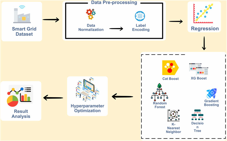
Figure 1. Proposed framework.

3 Materials and methods

This part gives an overview of the used methods and resources used in the research project in order to put the proposed solutions into practice. The combination of data preparation process and meta-heuristic optimization strategies makes it achievable to get to the best possible results.

3.1 Datasets

This dataset, which is addressed here, is the result of a thorough research work carried out by Angeliki Xifara (GitHub, 2019). The dataset was tweaked by Athanasios Tsanas, who is a member of the Oxford Centre for Industrial and Applied Mathematics at the University of Oxford, United Kingdom, as well. The direction of the research was high energy efficiency in building constructions. The Ecotect software was used in this study for the energy simulation of twelve different building forms. The basic difference between these building shapes was in terms of glazing area, glazing area distribution, glazing orientation, and other characteristics. They are making this dataset comprised of seven hundred and sixty-eight building configurations. The data sets are organized by using eight special features (X1 through X8) so that two continuous labels (y1 and y2) of heating and cooling load can be predicted easily.

These characteristics include the relative compactness (X1), the surface area (X2), the wall area (X3), the roof area (X4), the overall height (X5), the orientation (X6), the glazing area (X7), and the glazing area distribution (X8). A large dataset, it allows predicting energy loads with high precision, depending on the status of the response variables as continuous or discretized into nearest integers, and serves as a versatile resource for regression analysis and multi-class classification problems. This is true even if response variables are treated as continuous or discretized. These attributes are used to aid precise forecasts of heating and cooling requirements in buildings, which result in valuable inputs into the design of energy-effective structures by way of the application of computational modeling and optimization techniques.

3.2 Data preprocessing

The preprocessing of data is a crucial step that must be taken in order to improve the quality of the data and the performance of machine learning functions. At this level, the primary focus is on the application of techniques for normalization and data transformation. In the context of datasets pertaining to building energy efficiency, where the data ranges might be rather vast and may have a tendency to tilt towards larger values, discrepancies of this kind can have a negative impact on the performance of the model. Moreover, to overcome the problem, the research applies min-max normalization, which scales the data in a uniform method, thus making categorization algorithms more effective. Moreover, as numerical inputs are required for machine learning models, the preparation stage implies data encoding. This process of encoding turns categorical data into numbers, and this operation guarantees compatibility of this data with machine learning approaches. In this case, the dataset is then split into the training and test sets, the machine learning algorithms are trained on the training set, and their performance is measured on the test set. This study consists of 70% of the dataset for training purposes and the remaining 30% for testing and validation. Given the small size of the dataset, the study applies several machine learning algorithms for categorization. This reduces our dependence on deep learning strategies only. Methods that are used include Multilayer Perceptron (MLP), Extreme Gradient Boosting (XG Boost), Gradient Boosting (GB), Random Forest (RF), CatBoost (CB), Decision Tree (DT), and K Neighbors (KNN).

3.3 Basic classification models

A classification model aims to put data points into predefined categories accurately, and this is the engine behind such a model. These categories could be either binary categories with two classes or multi-class categories with three classes or even more. This is achieved through the use of different classification approaches.

3.3.1 K-nearest neighbor (KNN)

K-nearest neighbors algorithm is employed to classify a new data point in the feature space (El-Kenawy et al., 2022a). This method selects k neighbors, which are the closest to the end, and then assigns the label that is most represented among those neighbors to the end. The user chooses an integer k to use, and the user makes this choice. Although there are some other ways to measure the distance between the data points, the Euclidean distance is used most of the time. The Euclidean distance between two points in a multidimensional space is calculated using Eq. 1.

$d\left(p,q\right)={\left(q1-p1\right)}^2+{\left(q2-p2\right)}^2+\cdots +{\left(qn-pn\right)}^2(1)$

where p and q are two points in the n-dimensional space, and $p1,p2,\dots ,pnandq1,q2,\dots ,qn$ are their respective coordinates. are their respective coordinates (Zhao et al., 2021).

3.3.2 Gradient boosting (GB)

Gradient Boosting Machines (GBM) is a powerful model that is capable of solving regression and classification questions. Constant tuning of hyperparameters is essential for the GMB model because it allows control of the balance between underfit and overfit, which influences the model’s performance in the end. The key hyperparameters here are the number of trees, their depth, learning rate, and the minimum samples per leaf. The precise setting of the determining variables can drastically improve the accuracy of the model, thus resulting in a strategic methodology for assessing how those variables affect the model’s performance. This work proposes an understandable instruction that guides the user through the procedure of establishing and testing the mentioned parameters in Python in order to increase the accuracy of GBM models. This part of the response speaks of mechanical nets, especially the parameters, and also discusses the simple but effective tuning of the hyperparameter. A practitioner who wants to make the most of GBM for their job will find themselves at the right place with this guide on hand, which is just the thing for data scientists and machine learning lovers. The goal of cost function refinement aims to pick a weak learner that operates in the direction where the negative gradient of function is situated inside function space.

Boosting is an iterative approach in the ensemble learning context, which is designed to enhance prediction accuracy, taking advantage of a lot of weak learners. The output of the model at step t is updated according to the performance at the previous step t-1. Ignorance is bliss for the accurate predictions while the wrong predictions are punished. This approach is consistently used for classification problems with a similar method for regression cases. The boosting improves the learning process as it focuses on the difficult parts of the training data, which leads to the gradual improvement of the predictive accuracy of the model. Figure 2 demonstrates the idea of boosting. In boosting algorithms such as GBM or random forests, the parameters of an ensemble model are crucial in defining the model’s performance and behavior. These parameters can be classified into three main groups (Abediniangerabi et al., 2022).

1. Parameters specific to trees: These settings directly influence the organization and characteristics of individual trees in the ensemble. Important parameters for tree models are: Maximum depth: ensures the maximum level of trees. - Minimum samples split: the threshold number of splitting an internal node. - Minimum samples leaf: the minimum leaf node count. - Maximum number of features: the critical number to be sought when finding the best split (El-Kenawy et al., 2022b).

2. Boosting Parameters are crucial in the boosting process as they influence the construction and combination of the ensemble of trees. Key boosting parameters are the learning rate, which influences the impact of each tree on the final result and manages the pace of adjustment at each stage, the number of estimators representing the total trees in the model, and the subsample indicating the portion of samples for training each base learner. A subsample less than 1.0 introduces randomness to the model, aiding in avoiding overfitting.

3. Miscellaneous Parameters: These parameters cover other aspects of the model’s operation that are not directly related to tree construction or the boosting procedure. This may involve specifying the loss function to be optimized, setting the random state for the pseudo-random number generator used for random sampling to ensure reproducibility, and adjusting the verbosity level for the messages output during model training.

Figure 2

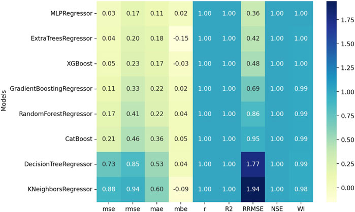
Figure 2. Comparative analysis of results regressor performance algorithms.

The WWPA is designed to be a repeatable process. Repositioning all waterwheels is the last step in adopting WWPA once the initial two stages are completed. The ideal solution candidate is enhanced after comparing target function values. The waterwheels’ positions are modified in each subsequent iteration until the algorithm reaches its final iteration.

3.3.3 Waterwheel plant algorithm (WWPA)

Specifically, it is a novel method of random optimization that is based on how natural systems work, as explained by (Abdelaziz et al., 2022). The WWPA is based on the idea that we should try to model how the waterwheel plant would act in its natural environment while it is hunting. This idea has been built on. The main idea behind WWPA came from the way that waterwheel plants find their insect prey, catch it, and then move it to a better spot to eat (Hussein Alkattan, S. K. Towfek, and M. Y. Shams, 2023). In the next part, we’ll talk about the ideas that led to the creation of the algorithm and the mathematical model that supports its methods.

3.3.3.1 Inspiration of the WWPA

Small transparent flytrap-like structures cover the broad petiole of the Waterwheel plant or Aldrovanda vesiculosa. Bristle-like hairs protect these 1/12-inch traps from damage or unintentional activation. The trap’s outside edges have hook-shaped teeth that interlock as it closes around its prey, like a flytrap. About forty elongated trigger hairs, like those in Venus’s flytraps, close the trap. To facilitate digestion, predators have acid-secreting glands. Interlocking teeth and a mucus sealant catch the victim and guide it to the trap’s base near the hinge. The trap digests the leftover water, absorbing most of the prey’s nutrition. Like flytraps, Aldrovanda traps can eat two to four meals before becoming dormant.

3.3.3.2 Mathematical model of WWPA

The WWPA is an iterative population-based approach that draws on the search capacity of its members throughout the Universe of possible solutions to identify an appropriate solution. According to their location in the search space, the WWPA population waterwheels’ problem variables have values. Therefore, every waterwheel stands for a solution that is built on vectors. The waterwheel population in the WWPA is shown by a matrix 2). Using (Eq. 2 and Eq. 3), WWPA randomly assigns water wheel sites to the search space at the outset.

$P=\left[\begin{array}{c}p1,1p1,2\dots p1,j\dots p1,m\\ p2,1p2,2\dots p2,j\dots p2,m\\ pi,1pi,2\dots pi,j\dots pi,m\\ pN,1pN,2...pN,j...pN,m\end{array}\right](2)$

$p_{i,j}={\text{lb}}_j+{\mathrm{r}}_{i,j}\left({\text{ub}}_j-{\text{lb}}_j\right),i=1:N,j=1:m(3)$

N is the number of waterwheels and m is the number of variables in this context. The jth variable in the issue has two limits, ${\text{lb}}_j$ and ${\text{ub}}_j$, and the value of ${\mathrm{r}}_{i,j}$ is a random number between 0 and 1. The waterwheel locations are stored in the population matrix, which is denoted by P. In the matrix, each row Pi stands for a potential solution, and $p_{i,j}$ represents the value of the jth variable for the ith waterwheel.

Every single waterwheel is taken into consideration as a potential solution to the issue, and as a result, the goal function can be evaluated for each and every one of them. It has been established in a previous study that a vector can be utilized to effectively express the values that constitute the objective function of the problem using Eq. 4.

$F=\left[\begin{array}{c}{F}_1\\ .\\ .\\ F_i\\ .\\ F_N\end{array}\right]=\left[\begin{array}{c}F\left(X_1\right)\\ \dots .\\ F\left(Xi\right)\\ \dots .\\ F\left(X_N\right)\end{array}\right](4)$

The objective function values are contained in a vector F, with $F_i$ representing the estimated value for the ith waterwheel. Assessments of objective functions ascertain the optimal solutions. Therefore, the best candidate solution is represented by the highest value of the objective function, and the worst member is represented by the lowest value. Since the waterwheels traverse the search space at different speeds, the optimal solution evolves across iterations.

➢ Exploration

Waterwheels have a keen predatory instinct because of their advanced olfactory senses, allowing them to efficiently hunt and find pests. When an insect approaches the waterwheel, it immediately attacks and follows the victim by precisely determining its location. The WWPA utilizes a simulation of hunting behavior to represent the first stage of its population update mechanism. The WWPA improves its capacity to explore the optimal zone and prevent being stuck in local optima by integrating the waterwheel’s attack on the insect. Therefore, substantial changes in location happen inside the search area due to this modeling. An equation is used along with a simulation of the waterwheel’s movement towards the insect to find the new location of the waterwheel. If moving the waterwheel to this new position results in a higher value of the objective function, the old location is discarded in favor of the new one, a expressed by Eq. 5 and Eq. 6.

$\overrightarrow{\mathrm{W\hspace{0.17em}}}=\overrightarrow{r_1}\left(\overrightarrow{\mathrm{P\hspace{0.17em}}}\left(t\right)+2K\right)(5)$

${\overrightarrow{P}}_{t+1}=\overrightarrow{P}\left(t\right)+\overrightarrow{\mathrm{W\hspace{0.17em}}}\left(2K+\overrightarrow{r_2}\right)(6)$

If the solution fails to improve for three consecutive iterations, the position of the waterwheel can be altered using the following equation using Eq. 7.

${\overrightarrow{P}}_{t+1}=Gaussian\left({\mu }_P,\sigma \right)+\overrightarrow{r_1}\frac{\overrightarrow{P}\left(t\right)+2K}{\overrightarrow{\mathrm{W\hspace{0.17em}}}}(7)$

In this context, the variables $\overrightarrow{r_1}$ and $\overrightarrow{r_2}$ represent random variables with values ranging from 0 to 2 and 0 to 1, respectively. Furthermore, K is an exponential variable with values between 0 and 1. The vector $\overrightarrow{\mathrm{W\hspace{0.17em}}}$ denotes the diameter of the circle within which the waterwheel plant will explore for potential promising areas.

➢ Exploitation

WWPA’s second population update stage simulates waterwheels collecting and transferring insects to a feeding tube. During local search, WWPA exploits this simulated behavior to converge to appropriate solutions that are close to formerly found ones. The waterwheel’s search space position is somewhat altered by modeling the insect’s transit to the tube. WWPA designers initialize each waterwheel in the population with a random “good position for consuming insects,” mimicking waterwheels’ natural activity. Following the following equations, the waterwheel is relocated to the new location if the objective function value is higher, replacing the old location, as expressed by Eq. 8 and Eq. 9.

$\overrightarrow{\mathrm{W\hspace{0.17em}}}=\overrightarrow{r_3}*\left(K\overrightarrow{P_{best}}\left(t\right)+r_3\overrightarrow{P}\left(t\right)\right)(8)$

$\overrightarrow{P}\left(t+1\right)=\overrightarrow{\mathrm{P\hspace{0.17em}}}\left(t\right)+K\overrightarrow{\mathrm{W\hspace{0.17em}}}(9)$

In this scenario, $\overrightarrow{r_3}$ signifies a random variable with values alternating from 0 to 2. $\overrightarrow{P}\left(t\right)$ signifies the current solution at iteration t, while $\overrightarrow{P_{best}}$ represents the best solution attained thus far. Like exploration phase mentioned earlier, if the solution fails to advance for three repeated iterations, the following mutation is applied to ensure prevention of local minima as presented in Eq. 10.

$\overrightarrow{P}\left(t+1\right)=\left(\overrightarrow{r_1}+K\right)\mathit{sin}\left(\frac{FC}{\theta }\right)(10)$

where F and C are independent random variables with values among [-5,5]. Additionally, the next equation can be used to show the exponential decay of K, as expressed by Eq. 11.

$K=\left(1+\frac{{2t}^2}{{T_{\mathit{max}}}^3}+F\right)(11)$

The WWPA is provided as a method that can be carried out again and time again. The third and final stage of the WWPA implementation process involves adjusting the placements of all waterwheels. This phase comes after the first two stages have been completed. Following the comparison of the values of the target function, the candidate for the optimal solution is improved. Adjustments are made to the positions of the waterwheels for the subsequent iteration, and thus the process continues until the algorithm reaches its final iteration.

4 Simulation results

An exhaustive testing procedure is carried out in order to offer evidence that the suggested WWPA algorithm is both effective and superior. The experiments make use of Windows 10 and Python 3.9, both of which are executed at a frequency of three gigahertz on a processor that is an Intel Core i5 CPU. Experiments were conducted within the framework of a case study, and the findings entailed a comparison of the output of the ANN-WWPA approach to that of baseline models’ output on a dataset consisting of information on different buildings. The configuration settings of the WWPA as well as the settings of other optimization methodologies are presented in Table 1.

Table 1

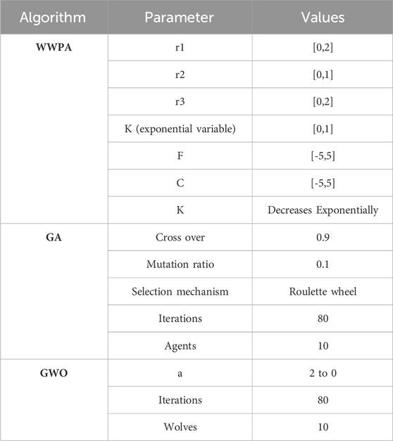
Table 1. Configuration parameters of the WWPA and competing optimization algorithms.

Regression models used to forecast energy efficiency in buildings incorporate additional metrics to assess their success (Almetwally and Amine, 2022; Alotaibi, et al., 2024). Among these measures are the following: RMSE, MAE, MBE, r, R², RRMSE, NSE, WI, and Pearson’s correlation coefficient. In this context, “N" stands for the overall count of observations in the dataset, $\left({\widehat{V}}_n\right)$ refers to the estimated and observed values for the $n^{\text{th}}$ bandwidth, and $\left(V_n\right)$ stands for the arithmetic means of the estimated and observed values, respectively. The criteria used to evaluate predictions are summarized in Table 2.

Table 2

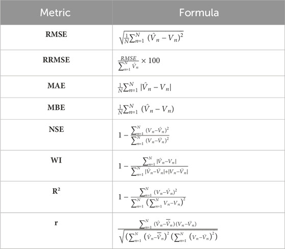
Table 2. Prediction evaluation criteria (Abdelaziz A., et al., 2023).

Table 3 shows that the XG Boost and MLP regressors outperformed other models on most metrics, including the MSE, RMSE, MAE, correlation R), and goodness-of-fit (R²). MLP has a flexible structure and can graph deep dependencies of the data set very likely so that it has the highest pattern-learning capabilities. The fact that it uses gradient boosting algorithms and an ensemble of decision trees makes XG Boost capable of handling both linear and non-linear interactions. This slow step in the fitting phase of the XGBoost is due to its ensemble nature, increasing the computational complexity that is achieved by the step of adding trees to the model.

Table 3

Table 3. Comparison of the performance metrics for different models.

When compared to MLP and XG Boost, Random Forest, Cat Boost, and Gradient Boosting all do decent work, but they cannot match MLP and XG Boost when it comes to efficiency and accuracy of predictions. These models use XG Boost-style ensemble learning approaches, which combine numerous weak learners into a strong model and typically produce robust performance. On the other hand, additional trees added to the ensemble may cause training times to slow down and overfitting to occur due to diminishing returns.

Although they are computationally efficient and use decision trees and K-Nearest Neighbors (KNN) models, ensemble approaches perform better. Decision Trees have a tendency to generate models that are too complicated and might not be able to apply them effectively to new data, which can result in increased error metrics. Although it is easy to see how KNN may work in theory, in practice it has problems with datasets that have a lot of characteristics or that have noisy data, which makes it less accurate at making predictions.

Table 4 discusses the results of applying different hyperparameter optimization techniques to MLP algorithm. The performance of several optimization techniques linked with the Multilayer Perceptron (MLP) regressor is highlighted by the findings obtained from the WWPA-MLP Regressor, the GWO-MLP Regressor, the GA-MLP Regressor, and the WOA-MLP Regressor. It is important to note that all of the models have incredibly low error measures, such as MSE, RMSE, and MAE, which indicates that they have a high level of prediction accuracy. The strong correlation R) and goodness-of-fit (R2) values, which approach or exceed 0.999 across all models, are a clear indication of the superior performance that has been achieved. It appears from this that the models are able to effectively capture the underlying relationships in the data, which ultimately results in exceptionally high prediction skills.

Table 4

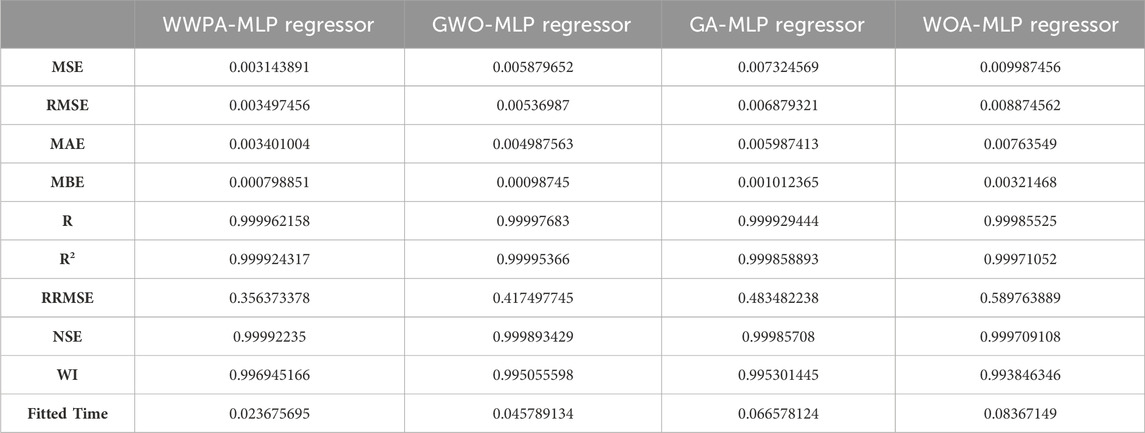
Table 4. Comparison of the performance metrics for different hyperparameter models.

In addition, the models have low relative errors to the magnitude of the forecasted magnitude, thus confirming their accuracy. It is shown by the rather low values of RRMSE, which is the abbreviation for relative root mean squared error. The values that were observed and the ones that were simulated were quite in agreement, as reflected by the Nash-Sutcliffe Efficiency (NSE) values, which are approaching 1. Furthermore, the high WI values tell us that the models are capable of correctly portraying the variability of the observed data.

It is gratifying to discover that, as predicted, there is an accuracy/computation efficiency trade-off. This is shown by the fact that the fitting time grows for all of the models. When compared to the WOA-MLP Regressor, which has the longest fitting time of 0.0837 s, the WWPA-MLP Regressor has the shortest fitting time of 0.0237 s. In light of this, it appears that although all models provide excellent prediction accuracy, the selection of one over another may be contingent on the particular requirements of the application, hence requiring a reasonable balance between precision and processing resources. In general, these findings provide evidence that demonstrates the effectiveness of employing a variety of optimization methods in conjunction with MLP regression in order to accomplish high-performance predictive modeling jobs.

The statistics that are presented in Table 5 for the WWPA-MLP Regressor, the GWO-MLP Regressor, the GA-MLP Regressor, and the WOA-MLP Regressor provide valuable insights into the distribution and features of the values that are anticipated. In each and every model, the number of values remains unchanged at 10, which is indicative of the fact that the size of the dataset is consistent. Values for the lowest, maximum, and range demonstrate the diversity in the forecasts. The WWPA-MLP Regressor has the smallest range, while the WOA-MLP Regressor exhibits the biggest range, indicating that there are disparities in the spread of the predictions.

Table 5

Table 5. Comparison of the performance metrics for different hyperparameter models.

All models display a level of confidence of 97.85%, as suggested by the confidence intervals, which provide information about the precision of the predictions. The mean and the standard deviation are two measures of central tendency and dispersion, respectively. These statistics indicate the mean value that was anticipated and the extent to which that value differed from the mean. It should be emphasized that the coefficient of variation represents the ratio of the variation in the predictions and that the WOA-MLP Regressor has the highest variation among the models.

The skewness and kurtosis information what the distribution looks like. The negative skewness value shows the left-skewed distribution. However, larger kurtosis values may suggest heavier tails and, therefore, more outliers within the distribution. The general aim of this data is to give a complete perspective on the predictability of each MLP regressor model, which involves the properties of their variability, accuracy, and distribution. This data is quite likely to be helpful when assessing the reliability and suitability of each of the models for individual forecasting tasks.

In most cases, the analysis of variance (ANOVA) provides an organized approach for determining the importance of treatment effects in experimental or observational research (Hiba and Almetwally, 2024). Using this model, investigators can derive actionable conclusions about the impact of different treatments or situations.

Table 6 enlightens on the amount of variation that exists within a dataset both between and across groups within the dataset. The “treatment” row (lying between columns) of this particular table gives the variance attributed to the different treatments or conditions being compared. In contrast, the “residual” row (lying between columns) shows the variation that cannot be explained within each treatment group. Sums of squares (SS) is used to measure the total variation, where Treatment SS expresses the variation that exists between treatment groups and Residual SS expresses the variation that exists within each treatment group by the treatment group. Treatment df is the number of treatment groups minus one, and residual df is the total number of observations minus the total number of treatment groups. The degree of freedom (DF) is an abstraction of the number of independent bits of information that are employed to infer a parameter or statistic. MS provides an estimate of the population variance. They are calculated by dividing the sum of squares by the degrees of freedom that are associated with the squares. The F statistic, which is obtained by dividing the Treatment MS by the Residual MS, gives the measure of the relative ratio of variability between treatment groups to variability within treatment groups.

Table 6

Table 6. ANOVA of the proposed feature selection method based on SG dataset.

This statistic is used to determine the mean of the treatment groups. The presence of a high F value indicates that the differences between treatment means are statistically significant in comparison to the variability that exists within treatment groups.

According to the null hypothesis, which states that there are no significant differences between treatment means, the p-value that is connected with the F statistic reflects the chance of receiving a F value that is as extreme as the one that was seen. In this particular instance, the p-value for the Treatment (between columns) is less than 0.0001, which indicates that there is substantial evidence against the null hypothesis and suggests that the variations between treatment means are statistically significant. Thus, we conclude that there are substantial differences between the treatment groups and reject the null hypothesis, which states that there are no differences.

A comparison of the medians of paired data samples is performed using the Wilcoxon Signed Rank Test as shown in Table 7 in order to ascertain whether or not there is a significant difference between the samples. In this scenario, the theoretical median, also known as the predicted value, is equal to zero for all models, however the actual median, also known as the observed value, differs from model to model.

Table 7

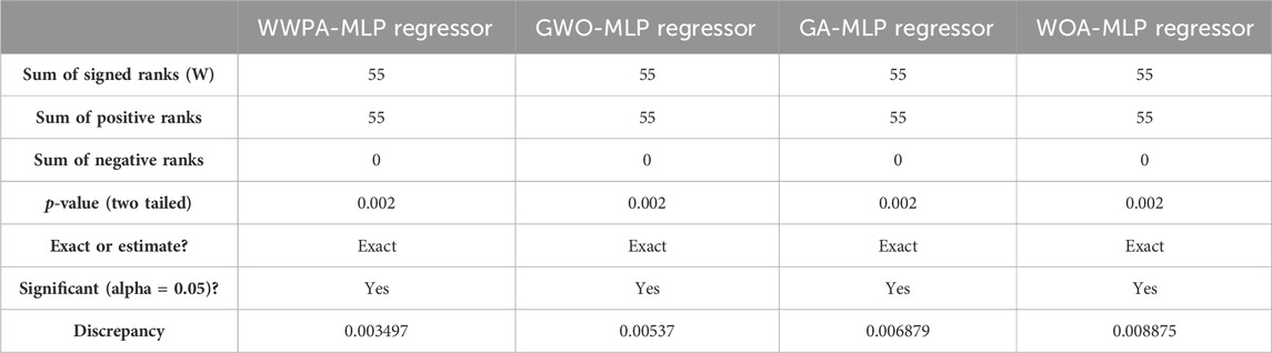
Table 7. Wilcoxon of the proposed feature selection method based on the EV population dataset.

One of the things that the test does is calculate the sum of signed ranks W) for each model. Positive ranks are allocated to differences in which the actual median is higher than the theoretical median, and negative ranks are assigned to differences in which the actual median is lower than the supposed median. The ideal situation would be for the sum of positive and negative ranks to be equal, which would indicate that there is no systematic bias in the differences.

The sum of signed ranks, denoted by the letter W, is equal to 55 for all models, along with the sum of both positive and negative ranks being equal to 55. This leads one to believe that there is no systemic bias in the discrepancies that exist between the theoretical medians and the actual medians for any different model.

At the two-tailed level, the p-value for each model is 0.002, which indicates that there is a significant difference between the medians that were predicted and those that were actually observed. Consequently, this indicates that the median values that were observed are significantly different from the median that was anticipated to be 0.

For the WWPA-MLP Regressor, the difference between the theoretical and real medians is 0.003497, for the GWO-MLP Regressor it is 0.00537, for the GA-MLP Regressor it is 0.006879, and for the WOA-MLP Regressor it is 0.008875. For each model, these discrepancies are a representation of the extent of the discrepancy between the median values that were expected and those that were actually observed. In general, the results of the Wilcoxon Signed Rank Test suggest that there are statistically significant variations between the theoretical and actual medians for all models. The values of the observed median are consistently higher than the theoretical median, which is 0.

A radar plot as shown in Figure 3 shows performance data for four MLP regressor models optimized by distinct algorithms: GWO, GA, WOA, and WWPA. Performance indicators including accuracy, precision, recall, F1 score, and mean squared error are shown on axes radiating from the plot center.

Figure 3

Figure 3. Comparative analysis of MLP Regressor performance optimized by evolutionary algorithms radar plot.

Various algorithms have been developed multilayer perceptron regression models, and this radar chart gives a visual comparison of them. It is possible to quickly evaluate the merits and shortcomings of each model because each point on the polygon represents a different performance statistic. The orange line, which may represent the WOA-MLP Regressor, stands out from the rest of the models in terms of how well they handle various criteria. This suggests that this model is the most comprehensive of the bunch. The green line represents the GA-MLP Regressor, and the blue line represents the WWO-MLP Regressor. These lines demonstrate variability across multiple measures, showing where the two models perform better or worse than each other. The red line, which stands for the WWPA-MLP Regressor, shows lower values in multiple measures. This could mean that the optimization strategy used to create this model is not optimal for the dataset.

Figure 4 provide a full diagnostic picture of the performance of the regression model. By displaying the residuals on the Y-axis as a function of the projected Y-values, the Residual plot, which can be found in the top left of the graph, reveals a random dispersion of data points. This indicates that the prediction is unbiased and that there are no apparent patterns, which is suggestive of a model that is well-fitted. Similarly, the Homoscedasticity plot is used to determine whether or not the residuals have the same amount of variance across all of the predicted values. If there is no visible trend or funnel shape in the scatter of dots, this indicates that the variance is consistent, which is a fundamental assumption of regression analysis. In the QQ plot, which is located below the Residual plot, the distribution of residuals is compared to a normal distribution. The data points closely align with the reference line, particularly in the central region, which indicates that the residuals are approximately normally distributed. This is a condition that, if it is not met, can significantly impact the validity of model inference. As a final point of discussion, the Heat Map on the right compares and contrasts various regression models (WWPA-MLP Regressor, GWO-MLP Regressor, GA-MLP Regressor, and WOA-MLP Regressor) by employing a color-coded system to represent a metric. This metric may be the magnitude of regression coefficients, or it may be model performance indicators such as error rates. Different models and parameters have different levels of intensity for the colors, which provides a visual depiction of the differences and similarities that might be used to guide the selection of the most appropriate regression method. It is essential to evaluate the performance and appropriateness of regression models for predictive analysis, and these diagnostics, when taken as a whole, are essential in verifying that the underlying assumptions are accurate for the data that is being considered.

Figure 4

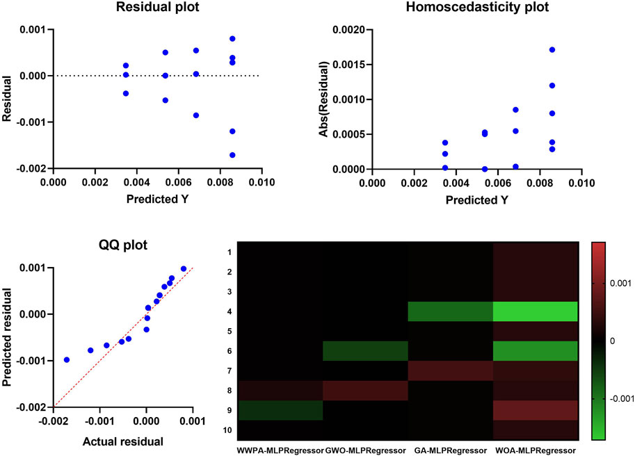
Figure 4. Visualizing the performance of the proposed feature selection method applied to SG dataset.

Figure 5 displays a comparison of various machine learning methods using the RMSE metric, a common way to assess the precision of a regression model. The RMSE or some other objective function shows how far off the model was from the real data, and it is plotted on the Y-axis. The four algorithms listed on the X-axis are WWPA-MLP Regressor, GWO-MLP Regressor, GA-MLP Regressor, and WOA-MLP Regressor. The RMSE from each iteration of the model’s training phase or a different fold of cross-validation is represented by a point in the scatter plot that shows each algorithm’s performance.

Figure 5

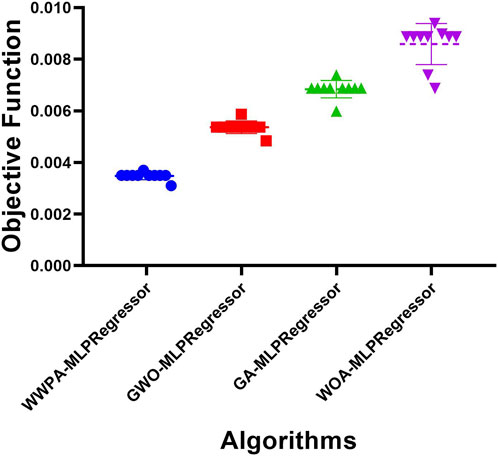
Figure 5. Comparative performance analysis of regression models using RMSE.

It would appear that the WWPA-MLP Regressor has the best spread and median RMSE, suggesting that its predictions are consistent and reliable across trials. A wider range of root-mean-squared errors (RMSEs) is seen in GA-MLP Regressor and the GWO-MLP Regressor, which may indicate less stability or greater sensitivity to the training data, respectively. The purple WOA-MLP Regressor has the largest spread and greatest median RMSE of the models, which may indicate that it is not as good at forecasting the target variable as the others.

Various MLP Regressors, each optimized using a different algorithm, are shown in the histogram shown in Figure 6.

Figure 6

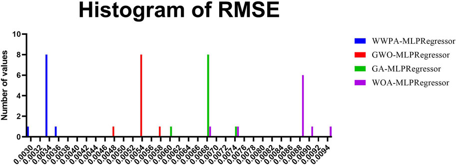
Figure 6. Comparative performance analysis of regression models using RMSE.

The WWP-MLP Regressor appears to successfully obtain low RMSE values on a consistent basis, which suggests that it may have a possibly superior predictive performance in comparison to the other models. Both the GWO-MLP Regressor and the GA-MLP Regressor have a greater range of RMSE values, which indicates that their performance is more variable.

RMSE can be relatively low or not, giving us an idea of the fluctuation amount and the model predictions’ accuracy. The try with the fact that the WWPA has a higher proportion of smaller RMSE values might be because the WWF is better in optimizing the MLP Regressor under the conditions that could be tested. In order to conduct a more comprehensive analysis of these findings, not only the proportion of low-value RMSE but also the stability and the computation effectiveness of all approaches should be considered.

5 Conclusion

In this work, we have demonstrated a novel methodology that harnesses the complementary strengths of ANNs and the WWPA for hyperparameter optimization, significantly enhancing the energy efficiency predictions in various buildings. This approach not only improves prediction accuracy across a diversity of building types and locations but also addresses the critical challenge of manual or generic hyperparameter selection in ANNs, marking a step forward towards achieving sustainability in the building industry. Our findings underscore the method’s practical relevance for property managers and construction professionals, offering a robust tool for advancing global sustainability goals through more precise energy efficiency forecasts and the facilitation of effective energy-saving initiatives.

Despite the model’s promising results, we acknowledge its dependence on high-quality input data and its initial limitation to specific building types and datasets. Looking ahead, we envision the integration of this methodology with digital twin technology, opening new avenues for real-time data analysis and further optimization of building energy efficiency. Such advancements could significantly broaden the model’s applicability and predictive accuracy across varied climatic conditions and architectural designs. Future research will aim to explore these possibilities, focusing on expanding the model’s versatility by incorporating additional predictive variables and employing cutting-edge optimization techniques. Our continued efforts will seek to refine and adapt this innovative approach, striving for a more inclusive and comprehensive tool that caters to the evolving needs of sustainable building practices.

Data availability statement

The original contributions presented in the study are included in the article/supplementary material, further inquiries can be directed to the corresponding authors.

Author contributions

AA: Writing–original draft, Writing–review and editing. DK: Writing–original draft, Writing–review and editing. AZ: Writing–original draft, Writing–review and editing. E-SE-K: Writing–original draft, Writing–review and editing. AI: Writing–original draft, Writing–review and editing. AA: Writing–original draft, Writing–review and editing. ME: Writing–original draft, Writing–review and editing. ME-S: Writing–original draft, Writing–review and editing. NK: Writing–original draft, Writing–review and editing. LA: Writing–original draft, Writing–review and editing. MS: Writing–original draft, Writing–review and editing.

Funding

The author(s) declare that financial support was received for the research, authorship, and/or publication of this article. Princess Nourah bint Abdulrahman University Researchers Supporting Project number (PNURSP 2024R120), Princess Nourah bint Abdulrahman University, Riyadh, Saudi Arabia.

Acknowledgments

Princess Nourah bint Abdulrahman University Researchers Supporting Project number (PNURSP 2024R120), Princess Nourah bint Abdulrahman University, Riyadh, Saudi Arabia.

Conflict of interest

The authors declare that the research was conducted in the absence of any commercial or financial relationships that could be construed as a potential conflict of interest.

Publisher’s note

All claims expressed in this article are solely those of the authors and do not necessarily represent those of their affiliated organizations, or those of the publisher, the editors and the reviewers. Any product that may be evaluated in this article, or claim that may be made by its manufacturer, is not guaranteed or endorsed by the publisher.

References

Abdelhamid, A. A. (2022). Machine learning-based model for talented students identification. J. Artif. Intell. Metaheuristics 1 (2), 31–41. doi:10.54216/JAIM.010204

CrossRef Full Text | Google Scholar

Abdelhamid, A. A., Eid, M. M., Abotaleb, M., and Towfek, S. K. (2023). Identification of cardiovascular disease risk factors among diabetes patients using ontological data mining techniques. J. Artif. Intell. Metaheuristics 4 (2), 45–53. doi:10.54216/JAIM.040205

CrossRef Full Text | Google Scholar

Abediniangerabi, B., Makhmalbaf, A., and Shahandashti, M. (2022). Estimating energy savings of ultra-high-performance fibre-reinforced concrete facade panels at the early design stage of buildings using gradient boosting machines. Adv. Build. Energy Res. 16 (4), 542–567. doi:10.1080/17512549.2021.2011410

CrossRef Full Text | Google Scholar

Ahmad, T., and Zhang, D. (2020). A critical review of comparative global historical energy consumption and future demand: the story told so far. Energy Rep. 6, 1973–1991. doi:10.1016/j.egyr.2020.07.020

CrossRef Full Text | Google Scholar

Al-Ghussain, L. (2019). Global warming: review on driving forces and mitigation. Environ. Prog. Sustain. Energy 38 (1), 13–21. doi:10.1002/ep.13041

CrossRef Full Text | Google Scholar

Almetwally, E. M., and Meraou, M. A. (2022). Application of environmental data with new extension of Nadarajah-Haghighi distribution. Comput. J. Math. Stat. Sci. 1 (1), 26–41. ‏. doi:10.21608/cjmss.2022.271186

CrossRef Full Text | Google Scholar

Alotaibi, R., Al-Dayian, G. R., Almetwally, E. M., and Rezk, H. (2024). Bayesian and non-Bayesian two-sample prediction for the Fréchet distribution under progressive type II censoring. AIP Adv. 14 (1). ‏. doi:10.1063/5.0174390

CrossRef Full Text | Google Scholar

Aqlan, F., Ahmed, A., Srihari, K., and Khasawneh, M. T. (2014). “Integrating artificial neural networks and cluster analysis to assess energy efficiency of buildings,” in IIE Annual Conference and Expo 2014, Montreal, Canada, 31 May - 3 June 2014, 3936–3943.

Google Scholar

Araújo, G. R., Teixeira, H., Gomes, M. G., and Rodrigues, A. M. (2023). Multi-objective optimization of thermochromic glazing properties to enhance building energy performance.

Google Scholar

Araújo, G. R., Teixeira, H., Gomes, M. G., and Rodrigues, A. M. (2022). Multi-objective optimization of thermochromic glazing properties to enhance building energy performance. Sol. Energy 249, 446–456. doi:10.1016/j.solener.2022.11.043

CrossRef Full Text | Google Scholar

Ascione, F., Bianco, N., Maria Mauro, G., and Napolitano, D. F. (2019). Building envelope design: multi-objective optimization to minimize energy consumption, global cost and thermal discomfort. Application to different Italian climatic zones. Energy 174, 359–374. doi:10.1016/j.energy.2019.02.182

CrossRef Full Text | Google Scholar

Boudjella, A., and Boudjella, M. Y. (2021a). “Cooling load energy performance of residential building: machine learning-cluster K-nearest neighbor CKNN (Part I),” in Lecture notes in networks and systems (vol. 174, issue Part I) (Springer International Publishing). doi:10.1007/978-3-030-63846-7_41

CrossRef Full Text | Google Scholar

Boudjella, A., and Boudjella, M. Y. (2021b). “Heating load energy performance of residential building: machine learning-cluster K-nearest neighbor CKNN (Part I),” in Lecture notesin networks and systems (vol. 174, issue Part I) (Springer International Publishing). doi:10.1007/978-3-030-63846-7_41

CrossRef Full Text | Google Scholar

Caroprese, L., Pierantozzi, M., Lops, C., and Montelpare, S. (2024). DL2F: a deep learning model for the local forecasting of renewable sources. Comput. Industrial Eng. 187, 109785. doi:10.1016/j.cie.2023.109785

CrossRef Full Text | Google Scholar

Chou, J. S., and Bui, D. K. (2014). Modeling heating and cooling loads by artificial intelligence for energy-efficient building design. Energy Build. 82 (2014), 437–446. doi:10.1016/j.enbuild.2014.07.036

CrossRef Full Text | Google Scholar

Chung, M. H., and Rhee, E. K. (2014). Potential opportunities for energy conservation in existing buildings on university campus: a field survey in Korea. Energy Build. 78, 176–182. doi:10.1016/j.enbuild.2014.04.018

CrossRef Full Text | Google Scholar

Dahiya, N., Gupta, S., and Singh, S. (2022). A review paper on machine learning applications, advantages, and techniques. ECS - Electrochem. Soc. 107 (1), 6137–6150. doi:10.1149/10701.6137ecst

CrossRef Full Text | Google Scholar

Dogan, A., and Birant, D. (2021). Machine learning and data mining in manufacturing. Expert Syst. Appl. 166, 114060. September 2020. doi:10.1016/j.eswa.2020.114060

CrossRef Full Text | Google Scholar

Eid, M. M., El-Kenawy, E. S. M., Khodadadi, N., Mirjalili, S., Khodadadi, E., Abotaleb, M., et al. (2022). Meta-heuristic optimization of LSTM-based deep network for boosting the prediction of monkeypox cases. Mathematics 10 (20), 3845. doi:10.3390/math10203845

CrossRef Full Text | Google Scholar

El-kenawy, E. M., Ibrahim, A., Mirjalili, S., Zhang, Y., Elnazer, S., and Zaki, R. M. (2022a). Optimized ensemble algorithm for predicting metamaterial antenna parameters. Comput. Mater. Continua 71 (3), 4989–5003. doi:10.32604/cmc.2022.023884

CrossRef Full Text | Google Scholar

El-Kenawy, E. S. M., Zerouali, B., Bailek, N., Bouchouich, K., Hassan, M. A., Almorox, J., et al. (2022b). Improved weighted ensemble learning for predicting the daily reference evapotranspiration under the semi-arid climate conditions. Environ. Sci. Pollut. Res. 29 (54), 81279–81299. doi:10.1007/s11356-022-21410-8

CrossRef Full Text | Google Scholar

Ersoz, B., Sagiroglu, S., and Bulbul, H. I. (2022). “A short review on explainable artificial intelligence in renewable energy and resources,” in 11th IEEE International Conference on Renewable Energy Research and Applications, ICRERA 2022, Istanbul, Turkey, 18-21 September 2022, 247–252.

CrossRef Full Text | Google Scholar

Esfe, M. H., Kamyab, M. H., and Toghraie, D. (2022). Statistical review of studies on the estimation of thermophysical properties of nanofluids using artificial neural network (ANN). Powder Technol. 400, 117210. doi:10.1016/j.powtec.2022.117210

CrossRef Full Text | Google Scholar

Goliatt, L., Capriles, P. V. Z., and Duarte, G. R. (2018). “Modeling heating and cooling loads in buildings using Gaussian processes,” in 2018 IEEE Congress on Evolutionary Computation, CEC 2018 - Proceedings, Rio de Janeiro, Brazil, 8-13 July 2018.

CrossRef Full Text | Google Scholar

Guo, T., and Li, X. (2023). Machine learning for predicting phenotype from genotype and environment. Curr. Opin. Biotechnol. 79, 102853. doi:10.1016/j.copbio.2022.102853

PubMed Abstract | CrossRef Full Text | Google Scholar

Hassan, S. U., Ahamed, J., and Ahmad, K. (2022). Analytics of machine learning-based algorithms for text classification. Sustain. Operations Comput. 3, 238–248. July 2021. doi:10.1016/j.susoc.2022.03.001

CrossRef Full Text | Google Scholar

Hernandez-Matheus, A., Löschenbrand, M., Berg, K., Fuchs, I., Aragüés-Peñalba, M., BullichMassagué, E., et al. (2022). A systematic review of machine learning techniques related to local energy communities. Renew. Sustain. Energy Rev. 170, 112651. October. doi:10.1016/j.rser.2022.112651

CrossRef Full Text | Google Scholar

Hussein, A., Towfek, S. K., and Shams, M. Y. (2023). Tapping into knowledge: ontological data mining approach for detecting cardiovascular disease risk causes among diabetes patients. J. Artif. Intell. Metaheuristics 4 (1), 08–15. doi:10.54216/JAIM.040101

CrossRef Full Text | Google Scholar

Invidiata, A., Lavagna, M., and Ghisi, E. (2018). Selecting design strategies using multi-criteria decision making to improve the sustainability of buildings. Build. Environ. 139, 58–68. November 2017. doi:10.1016/j.buildenv.2018.04.041

CrossRef Full Text | Google Scholar

Irfan, M., and Ramlie, F. (2021). Analysis of parameters which affects prediction of energy consumption in buildings using partial least square (PLS) approach. J. Adv. Res. Appl. Sci. Eng. Technol. 25 (1), 61–68. doi:10.37934/araset.25.1.6168

CrossRef Full Text | Google Scholar

Karatzas, K., and Katsifarakis, N. (2018). Modelling of household electricity consumption with the aid of computational intelligence methods. Adv. Build. Energy Res. 12 (1), 84–96. doi:10.1080/17512549.2017.1314831

CrossRef Full Text | Google Scholar

Khafaga, D., Ali Alhussan, A., M. El-kenawy, E. S., E. Takieldeen, A., M. Hassan, T., A. Hegazy, E., et al. (2022). Meta-heuristics for feature selection and classification in diagnostic Breast燙ancer. Comput. Mater. Continua 73 (1), 749–765. doi:10.32604/cmc.2022.029605

CrossRef Full Text | Google Scholar

Kim, D. D., and Suh, H. S. (2021). Heating and cooling energy consumption prediction model for high-rise apartment buildings considering design parameters. Energy Sustain. Dev. 61, 1–14. doi:10.1016/j.esd.2021.01.001

CrossRef Full Text | Google Scholar

Liapikos, T., Zisi, C., Kodra, D., Kademoglou, K., Diamantidou, D., Begou, O., et al. (2022). Quantitative structure retention relationship (QSRR) modelling for Analytes’ retention prediction in LC-HRMS by applying different Machine Learning algorithms and evaluating their performance. J. Chromatogr. B 1191, 123132. doi:10.1016/j.jchromb.2022.123132

CrossRef Full Text | Google Scholar

Lokhandwala, M., and Nateghi, R. (2018). Leveraging advanced predictive analytics to assess commercial cooling load in the U.S. Sustain. Prod. Consum. 14, 66–81. doi:10.1016/j.spc.2018.01.001

CrossRef Full Text | Google Scholar

Lops, C., Pierantozzi, M., Caroprese, L., and Montelpare, S. (2023). “A deep learning approach for climate parameter estimations and renewable energy sources,” in 2023 IEEE International Conference on Big Data (BigData), Sorrento, Italy, December 15-18, 2023 (IEEE), 3942–3951.

CrossRef Full Text | Google Scholar

Machlev, R., Heistrene, L., Perl, M., Levy, K. Y., Belikov, J., Mannor, S., et al. (2022). Explainable Artificial Intelligence (XAI) techniques for energy and power systems: review, challenges and opportunities. Energy AI 9, 100169. doi:10.1016/j.egyai.2022.100169

CrossRef Full Text | Google Scholar

Mastrucci, A., van Ruijven, B., Byers, E., Poblete-Cazenave, M., and Pachauri, S. (2021). Global scenarios of residential heating and cooling energy demand and CO2 emissions. Clim. Change 168 (3–4), 14–26. doi:10.1007/s10584-021-03229-3

CrossRef Full Text | Google Scholar

Medal, L. A., Sunitiyoso, Y., and Kim, A. A. (2021). Prioritizing decision factors of energy efficiency retrofit for facilities portfolio management. J. Manag. Eng. 37 (2), 1–12. doi:10.1061/(asce)me.1943-5479.0000878

CrossRef Full Text | Google Scholar

Mishra, P., Swain, B. R., and Swetapadma, A. (2022). “A review of cancer detection and prediction based on supervised and unsupervised learning techniques,” in Smart healthcare analytics: state of the art. Editors P. K. Pattnaik, A. Vaidya, S. Mohanty, S. Mohanty, and A. Hol (Singapore: Springer), 21–30. doi:10.1007/978-981-16-5304-9_3

CrossRef Full Text | Google Scholar

Moayedi, H., and Mosavi, A. (2021). Suggesting a stochastic fractal search paradigm in combination with artificial neural network for early prediction of cooling load in residential buildings. Energies 14 (6), 1649. doi:10.3390/en14061649

CrossRef Full Text | Google Scholar

Mokeev, V. V. (2019). “Prediction of heating load and cooling load of buildings using neural network,” in Proceedings - 2019 International Ural Conference on Electrical Power Engineering, UralCon 2019, Chelyabinsk, Russia, 1-3 October 2019, 417–421.

CrossRef Full Text | Google Scholar

Muhammed, H. Z., and Almetwally, E. M. (2024). Bayesian and non-bayesian estimation for the shape parameters of new versions of bivariate inverse weibull distribution based on progressive type II censoring. Comput. J. Math. Stat. Sci. 3 (1), 85–111. doi:10.21608/cjmss.2023.250678.1028

CrossRef Full Text | Google Scholar

Nazir, A., Wajahat, A., Akhtar, F., Ullah, F., Qureshi, S., Malik, S. A., et al. (2020). “Evaluating energy efficiency of buildings using artificial neural networks and K-means clustering techniques,” in 2020 3rd International Conference on Computing, Mathematics and Engineering Technologies: Idea to Innovation for Building the Knowledge Economy, ICoMET 2020, Sukkur, Pakistan, 29-30 January 2020.

CrossRef Full Text | Google Scholar

Phan, L., and Lin, C. X. (2014). A multi-zone building energy simulation of a data center model with hot and cold aisles. Energy Build. 77, 364–376. doi:10.1016/j.enbuild.2014.03.060

CrossRef Full Text | Google Scholar

Pierantozzi, M., and Hosseini, S. M. (2024). Density and viscosity modeling of liquid adipates using neural network approaches. J. Mol. Liq. 397, 124134. doi:10.1016/j.molliq.2024.124134

CrossRef Full Text | Google Scholar

Piras, G., Agostinelli, S., and Muzi, F. (2024). Digital twin framework for built environment: a review of key enablers. Energies 17 (2), 436. doi:10.3390/en17020436

CrossRef Full Text | Google Scholar

Piras, G., and Muzi, F. (2024). Energy transition: semi-automatic BIM tool approach for elevating sustainability in the maputo natural history museum. Energies 17 (4), 775. doi:10.3390/en17040775

CrossRef Full Text | Google Scholar

Prasetiyo, B., and Muslim, M. A. (2019). Analysis of building energy efficiency dataset using naive bayes classification classifier. J. Phys. Conf. Ser. 1321 (3), 032016. doi:10.1088/1742-6596/1321/3/032016

CrossRef Full Text | Google Scholar

Pruneski, J. A., Pareek, A., Kunze, K. N., Martin, R. K., Karlsson, J., Oeding, J. F., et al. (2022). Supervised machine learning and associated algorithms: applications in orthopedic surgery. Knee Surg. Sports Traumatol. Arthrosc. 31 (4), 1196–1202. doi:10.1007/s00167-022-07181-2

PubMed Abstract | CrossRef Full Text | Google Scholar

Renuka, S. M., Maharani, C. M., Nagasudha, S., and Raveena Priya, R. (2022). Optimization of energy consumption based on orientation and location of the building. Mater. Today:Proceedings 65, 527–536. doi:10.1016/j.matpr.2022.03.081

CrossRef Full Text | Google Scholar

Rodríguez, M. V., Cordero, A. S., Melgar, S. G., and Andújar Márquez, J. M. (2020). Impact of global warming in subtropical climate buildings: future trends and mitigation strategies. Energies 13 (23), 1–22. doi:10.3390/en13236188

CrossRef Full Text | Google Scholar

Samee, N. A., El-Kenawy, E. S. M., Atteia, G., Jamjoom, M. M., Ibrahim, A., Abdelhamid, A. A., et al. (2022). Metaheuristic optimization through deep learning classification of COVID-19 in chest X-ray images. Comput. Mater. Continua 73 (2). doi:10.32604/cmc.2022.031147

CrossRef Full Text | Google Scholar

Selvalakshmi, S., Immanual, R., Priyadharshini, B., and Sathya, J. (2022). Artificial neural network (ANN) modelling for the thermal performance of bio fluids. Mater. Today Proc. 66, 1289–1294. doi:10.1016/j.matpr.2022.05.128

CrossRef Full Text | Google Scholar

Shanthi, J., and Srihari, B. (2018). Prediction of heating and cooling load to improve energy efficiency of buildings using machine learning techniques. J. Mech. Continu Math. Sci. 13 (5). doi:10.26782/jmcms.2018.12.00008

CrossRef Full Text | Google Scholar

Tsanas, A., and Xifara, A. (2012). Accurate quantitative estimation of energy performance of residential buildings using statistical machine learning tools. Energy Build. 49, 560–567. doi:10.1016/j.enbuild.2012.03.003

CrossRef Full Text | Google Scholar

Tsoka, T., Ye, X., Chen, Y. Q., Gong, D., and Xia, X. (2022). Explainable artificial intelligence for building energy performance certificate labelling classification. J. Clean. Prod. 355, 131626. December 2021. doi:10.1016/j.jclepro.2022.131626

CrossRef Full Text | Google Scholar

van der Velden, B. H. M., Kuijf, H. J., Gilhuijs, K. G. A., and Viergever, M. A. (2022). Explainable artificial intelligence (XAI) in deep learning-based medical image analysis. Med. Image Anal. 79, 102470. doi:10.1016/j.media.2022.102470

PubMed Abstract | CrossRef Full Text | Google Scholar

Xie, Y., Wu, D., Dong, B., and Li, Q. (2022). Trained model in supervised deep learning is a conditional risk minimizer. Available at: http://arxiv.org/abs/2202.03674.

Google Scholar

Xu, X., Taylor, J. E., Pisello, A. L., and Culligan, P. J. (2012). The impact of place-based affiliation networks on energy conservation: an holistic model that integrates the influence of buildings, residents and the neighborhood context. Energy Build. 55, 637–646. doi:10.1016/j.enbuild.2012.09.013

CrossRef Full Text | Google Scholar

Yoro, K. O., and Daramola, M. O. (2020). “CO2 emission sources, greenhouse gases, and the global warming effect,” in Advances in carbon capture (Elsevier Inc). doi:10.1016/b978-0-12-819657-1.00001-3

CrossRef Full Text | Google Scholar

Yu, T., Boob, A. G., Volk, M. J., Liu, X., Cui, H., and Zhao, H. (2023). Machine learning-enabled retrobiosynthesis of molecules. Nat. Catal. 6 (2), 137–151. doi:10.1038/s41929-022-00909-w

CrossRef Full Text | Google Scholar

Zhang, C., and Lu, Y. (2021). Study on artificial intelligence: the state of the art and future prospects. J. Industrial Inf. Integration 23, 100224. March. doi:10.1016/j.jii.2021.100224

CrossRef Full Text | Google Scholar

Zhang, Y., Teoh, B. K., Wu, M., Chen, J., and Zhang, L. (2023). Data-driven estimation of building energy consumption and GHG emissions using explainable artificial intelligence. Energy 262 (PA), 125468. doi:10.1016/j.energy.2022.125468

CrossRef Full Text | Google Scholar

Zhao, D., Hu, X., Xiong, S., Tian, J., Xiang, J., Zhou, J., et al. (2021). K-means clustering and kNN classification based on negative databases. Appl. soft Comput. 110, 107732. doi:10.1016/j.asoc.2021.107732

CrossRef Full Text | Google Scholar