Research on the optimization of belief rule bases using the Naive Bayes theory

1 Introduction

The belief rule-based expert system integrates rule parameters on the basis of traditional IF-THEN rules, aiming to model the system using semi-quantitative information. Through this approach, it has the convenience of expert knowledge expression in the knowledge base without the need for a complete understanding of the structure. However, for a multi-rule system and in the context of a dynamic system, there are time-scale differences among the multiple variables’ symptoms. Therefore, the initial belief rule-based system established by domain experts needs to be continuously improved by fault samples to enhance the timeliness and accuracy of fault diagnosis.

There is a considerable amount of research both domestically and internationally on expert systems using the belief rule base. Yang et al. (2006), building upon the Dempster–Shafer (D-S) theory, fuzzy theory, and IF-THEN rule statements, developed a belief rule-based reasoning method based on evidence reasoning. Zheng et al. (2018) modeled the fault mechanisms to obtain a set of fault-related symptom parameters. Using mathematical statistics combined with relevant field experience, the construction of an expert rule base for diagnosing high-pressure heater pipe leakage faults is accomplished. Ahmed et al. (2020) developed a belief rule-based expert system designed to forecast the severity of four types of coronary artery diseases in advance, achieving a success rate of 93.97%. Chen et al. (2018) constructed a fuzzy-weighted production rule inference engine based on an intelligent soot-blowing expert system. The weights of various feature parameters were determined using an improved analytic hierarchy process (AHP). Through the weighted fusion of multiple data points, the belief rule-based system was further optimized. However, there are still issues with the current use of belief rule-based expert systems for intelligent equipment diagnosis: (1) multiple fault symptoms related to multiple antecedent attributes are different when an actual fault occurs, significantly impacting the timeliness and accuracy of fault diagnosis. Consequently, this diminishes diagnostic efficiency. (2) The key parameters of the belief rule-based system, specifically the threshold and limit values, are fixed values dependent on expert experience. The lack of self-learning capability imposes certain limitations on the system.

Gaussian mixture clustering is a target function-based clustering method initially introduced by Wolfe (1963). The Gaussian mixture model (GMM) was further extended from field of density estimation to the clustering domain by McLachlan and Basford (1988). The application scope of Gaussian mixture clustering has since expanded significantly, encompassing diverse areas such as speech recognition, image classification, fault diagnosis (Xiao et al., 2011; Gao et al., 2020), and motion target detection (Lv and Sun, 2019; Li et al., 2020). Its wide-ranging applications validate the strong adaptability of this method.

The essence of Bayesian theory lies in determining the probability of the intrinsic attributes of a global incident based on the probability of the occurrence of local incidents. In other words, it infers the characteristics of the whole from the characteristics of the sample. Bayesian classification is a common statistical-based classification method. However, when the dataset contains a large number of variables, the model structure becomes extremely complex, and computation time significantly increases, resulting in low classification efficiency. To address this issue, the Naive Bayes classification algorithm was introduced. In 1988, Bayesian belief networks (BBNs) were introduced by Pearl (1988). This algorithm applies probability and statistical theory to complex domains, facilitating uncertainty reasoning and analysis. It characterizes relationships between attributes, thereby enhancing the accuracy of classification. Frank et al. (2002) proposed the local weighted Naive Bayes, which selected the nearest neighbor samples for each test sample and treated them as the testing set. By combining this with the Naive Bayes classifier, the algorithm improves classification accuracy. Zhang and Guo (2015), while retaining the simplicity of the Naive Bayes classification algorithm, assigned different weights to various attributes based on association rules mined from text and their confidence, effectively enhancing its performance.

This paper focuses on intelligent fault diagnosis using a belief rule-based expert system, combining the Naive Bayes model and Gaussian mixture clustering to optimize the belief rule-based system. Fault data samples are divided into multiple windows. Gaussian mixture clustering is used for each window to determine the threshold and limit values for the window data. These threshold and limit values for each window are treated as labels, while the data for each window serve as samples. Together, they are input into the Naive Bayes model for training; subsequently, another window of fault data is taken and input into the trained Naive Bayes model. The output of the corrected threshold and limit values is obtained. These values are updated across the entire belief rule-based system. Using fault timeliness as a criterion, if the diagnostic time significantly advances, belief rule-based optimization is completed; otherwise, iteration over threshold and limit values is continued. By optimizing the belief rule-based approach presented in this paper, the timeliness of fault diagnosis is improved, leading to enhanced diagnostic efficiency. This method breaks away from relying solely on fixed values based on expert experience for threshold and limit values in the belief rule-based system. Finally, through practical validation, it has been demonstrated that this approach can improve the timeliness and accuracy of fault diagnosis, particularly in cases where multiple fault symptoms related to multiple antecedent attributes are different.

2 Establishment of the belief rule base for fault diagnosis

The belief rule base is used to store domain expert-related knowledge in a specific format. In the field of fault diagnosis, the first step involves establishing a fault model through mechanism analysis to identify the primary fault symptoms. This process is complemented by incorporating experiential knowledge from domain experts to acquire additional symptoms associated with fault types. Thereby, a belief rule base for the fault diagnosis expert system is constructed, establishing a one-to-one mapping relationship between fault types and multiple fault symptoms.

2.1 Using the belief rule base in the fault diagnosis process

The specific description of the kth rule in the belief rule base for fault diagnosis is provided in this article as follows:

$R_k:IF{x}_{1}is{A}_1^k\wedge x_{2}is{A}_2^k\wedge \cdots \wedge x_{\mathrm{M}}is{A}_{\mathrm{M}}^{k}Then\left(D_k,{\beta }_k\right).(1)$

In Eq. 1, k represents that this belief rule is the kth rule in the belief rule base. $A_i^k$ indicates the reference values for the antecedent attributes; x_i ($i=1,2,\dots ,M$) represents the ith input vector; and M indicates the number of fault symptoms in the kth rule. $\left\{A_1^K,A_2^K,\cdots A_M^K\right\}$ represent the set formed by the reference values of antecedent attributes in the kth rule of the belief rule base. $\left(D_k,{\beta }_k\right)$ indicate the output result after applying the reference values of input in the kth rule, where $D_k$ represents the output fault type and ${\beta }_k$ denotes the confidence level of the conclusion for the fault type.

Through the reference values of antecedent attributes $A_i^k\left(\overline{x_i},\overline{{\delta }_i},c_{i_1},c_{i_2}\right)$ and the corresponding membership functions, evidence confidence ${\delta }_i^{\prime }$ for input symptom x_i can be calculated, where $\overline{{\delta }_{\mathrm{i}}}$ represents the preset confidence level of the antecedent attribute (condition) and $xi$ represents the actual value of feature $\overline{x_i}$. $c_{i_1}$ is the threshold value for the symptom, and $c_{i_2}$ is the limit value for the symptom.

For input variable $xi$, the fuzzy membership function in this article is a linear membership function, and combining the threshold $c_{i_1}$, limit $c_{i_2}$, and fuzzy membership function, the evidence confidence ${\delta }_i^{\prime }$ corresponding to x_i is calculated.

Once the evidence confidence ${\delta }_i^{\prime }$ for symptom x_i is obtained, the matching degree ${\theta }_k$ for the current rule k can be calculated in Eq. 2:

${\theta }_k=\mathit{max}\left\{0,\overline{{\delta }_1}-{\delta }_1^{\prime }\right\}+\mathit{max}\left\{0,\overline{{\delta }_1}-{\delta }_2^{\prime }\right\}+\cdots +\mathit{max}\left\{0,\overline{{\delta }_M}{-\delta }_M^{\prime }\right\}<\epsilon .(2)$

In the above equation, ${\theta }_k$ represents the matching degree for the current rule k, and $\epsilon$ denotes the matching index, which is set based on expert experience; $\overline{{\delta }_i}\left(i=1,2,\cdots ,M\right)$ represent the preset confidence level for the antecedent attributes of the rule. If ${\theta }_k$ is less than $\epsilon$, it indicates that the matching degree for the current rule is less than the specified matching threshold. The matching result is true, and the confidence in matching for the conclusion is then computed. Otherwise, the matching result is false. The calculation for conclusion confidence is Eq. 3:

$\beta =\left[1-\mathit{max}\left\{0,\overline{{\delta }_1}-{\delta }_1^{\prime }\right\}\right]\times \left[1-\mathit{max}\left\{0,\overline{{\delta }_1}-{\delta }_2^{\prime }\right\}\right]\times \cdots \left[1-\mathit{max}\left\{0,\overline{{\delta }_M}{-\delta }_M^{\prime }\right\}\right]\times \stackrel{\sim }{\beta }.(3)$

In the above equation, $\stackrel{\sim }{\beta }$ represents the preset confidence level for the fault conclusion.

The belief rule base formed based on the expert system has certain limitations due to multiple fault symptoms related to multiple antecedent attributes being different, resulting in slow diagnostic times. This paper adopts Gaussian mixture clustering, and Naive Bayes theory iteratively learns the threshold $c_{i_1}$ and limit $c_{i_2}$ for fault symptoms in the belief rule base. The inference calculation process of the belief rule base is shown in Figure 1.

Figure 1

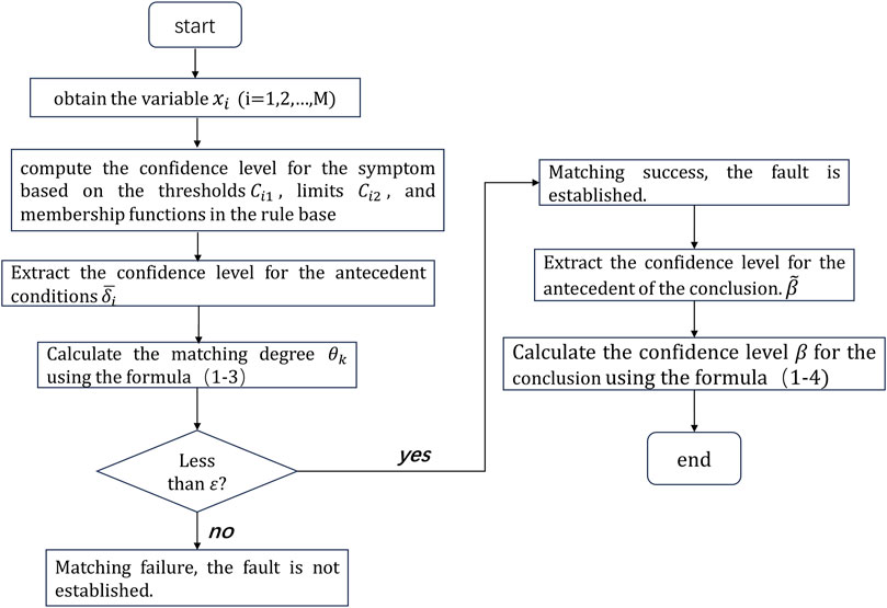
Figure 1. Inference calculation process of the belief rule base.

3 Belief rule-based optimization for fault diagnosis

This paper will integrate the theory of Naive Bayes and iteratively optimize the thresholds $c_{i_1}$ and limits $c_{i_2}$ in the belief rule base to enhance the timeliness and accuracy of fault diagnosis results. The essence of Bayesian theory lies in determining the probability of the intrinsic attributes of a global incident based on the probability of the occurrence of local incidents. When analyzing a sample that is sufficiently large to approach the total sample size, the probability of incidents in the analyzed sample approaches the probability of incidents in the total sample. It is possible to infer the inherent attributes of the analyzed sample by examining the correlation between the analyzed and total samples. In this paper, the thresholds $c_{i_1}$ and limits $c_{i_2}$ for the analyzed sample are derived by analyzing the correlation between the analyzed and total samples.

A specific fault type is selected, and the historical operational data of various fault symptoms associated with that fault type as training sample D are used. The sliding window method is applied to partition the data sample D. It is divided into n windows, each with a width of L. $D=\left\{W_1,W_2,\cdots W_n\right\}$.

Gaussian mixture clustering is performed on the fault symptom data $W_i$ in each window to obtain the thresholds $c_{i_1}$ and limits $c_{i_2}$ for each fault symptom under that fault type in each window. $W_i=\left\{x_1,x_2,\cdots x_m\right\}$. The fault data from each window are used as training samples, inputting both the thresholds $c_{i_1}$ and limits $c_{i_2}$ corresponding to each window as labels into the Naive Bayes model. Then, another window is taken from a set of fault samples and input into the trained Bayesian model. The corrected thresholds $c_{k_1}$ and limits $c_{k_2}$ are calculated based on the correlation between this sample and the overall sample. The original thresholds $c_{i_1}$ and limits $c_{i_2}$ are replaced in the rule base with the new thresholds $c_{k_1}$ and limits $c_{k_2}$, respectively, iterating through all fault symptoms and sequentially completing the threshold and limit adjustments for all fault symptoms under that fault type. This process forms a completely new rule base. The third set of fault data is used to compare the diagnostic times between the original rule base and the new rule base. If the diagnostic time using the original rule base is ahead of the diagnostic time using the new rule base, iteration is continued. Otherwise, the optimization of the belief rule base is considered complete.

3.1 Threshold and limit calculation based on Gaussian mixture clustering

Gaussian mixture clustering uses a probabilistic model to express clustering prototypes. The definition of a (multivariate) Gaussian distribution is as follows: for a random vector x in the n-dimensional sample space X, if x follows a Gaussian distribution, then the probability density function of x is given using the following equation:

$R_k:IF{x}_{1}is{A}_1^k\wedge x_{2}is{A}_2^k\wedge \cdots \wedge x_{\mathrm{M}}is{A}_{\mathrm{M}}^{k}Then\left(D_k,{\beta }_k\right),(4)$

where $u$ is the n-dimensional mean vector and $\mathrm{\Sigma }$ is the $n\times n$ covariance matrix. From Eq. 4, it is evident that the Gaussian distribution is established solely by the parameters of the mean vector $\mu$ and the covariance matrix $\mathrm{\Sigma }$. To facilitate the representation of the relationship between the Gaussian distribution and its corresponding parameters, the probability density function of x is denoted as $p\left(x|\mu ,\mathrm{\Sigma }\right)$.

Thus, the definition of a Gaussian mixture distribution is given in Eq. 5

$p_M\left(x\right)={\displaystyle \sum _{i=1}^k}{\alpha }_i\cdot p\left(x\mid {\mu }_i,{\mathrm{\Sigma }}_i\right).(5)$

This distribution entails a total of k mixture components, each corresponding to a Gaussian distribution, where ${\mu }_i$ and ${\mathrm{\Sigma }}_i$ are the parameters of the ith Gaussian mixture component and $a_i>0$ is the “mixture coefficient” corresponding to that parameter. Furthermore, there exists $\sum _{i=1}^k{a}_i=1$.

Assuming the birth process of the samples is determined using a Gaussian mixture distribution, first a Gaussian mixture component is selected according to the distribution defined previously as $a_1,a_2,\cdots ,a_k$, where $a_i$ is the probability of selecting the ith mixture component; upon selecting the mixture component, samples are drawn from its probability density function to generate the corresponding dataset.

Suppose the training set $W_i=\left\{x_1,x_2,\cdots x_m\right\}$ is derived from the above process. Let the random variable z_jö $\in$ {$1,2,\dots ,k$} represent the Gaussian mixture component for the jth sample x_j in the training set, and its value is unknown to us. The prior probability P (z_j = i) for z_j corresponds to $a_i$, where $i=1,2,\dots ,k$. According to Bayes’ theorem, the expression for the posterior distribution of z_j should be

$p_M\left(z_j=i\mid x_j\right)=\frac{P\left(z_j=i\right)\cdot p_M\left(x_j\mid z_j=i\right)}{p_M\left(x_j\right)}=\frac{{\alpha }_i\cdot p\left(x_j\mid {\mu }_i,{\mathrm{\Sigma }}_i\right)}{\sum _{l=1}^k{\alpha }_l\cdot p\left(x_j\mid {\mu }_l,{\mathrm{\Sigma }}_l\right)}.(6)$

In other words, it provides the posterior probability that sample x_j is generated by the ith Gaussian mixture component. For simplicity, let us denote it as γ_ji ($i=1,2,\dots ,k$).

When the Gaussian mixture distribution in Eq. 6 is known, Gaussian mixture clustering will partition the dataset (D) into k clusters E = {${\mathit{E}}_1,{\mathit{E}}_2,\dots ,{\mathit{E}}_k$}, and the cluster label λ_j for each sample x_j is determined, as shown in Eq. 7:

${\lambda }_j=\mathit{arg}\mathit{max}{\gamma }_{ji},i\in \left\{1,2,...,k\right\}.(7)$

Therefore, Gaussian mixture clustering describes prototypes using a probabilistic model based on the Gaussian distribution, and the cluster division is determined by the posterior probabilities corresponding to the prototypes.

So, for Eq. 6, the method of solving the model parameters {(α_i, μ_i, ∑_i)|1 ≤ i ≤ k}, setting the sample set D, can use maximum likelihood estimation. In other words, maximizing the (logarithm) likelihood, the calculation equation is as follows:

$LL\left(D\right)=\mathit{ln}\left({\displaystyle \prod _{j=1}^m}{p}_M\left(x_j\right)\right)={\displaystyle \sum _{j=1}^m}\mathit{ln}\left({\displaystyle \sum _{i=1}^k}{\alpha }_i\cdot p\left(x_j\mid {\mu }_i,{\mathrm{\Sigma }}_i\right)\right).(8)$

The expectation–maximization (EM) algorithm, a method for estimating parameters with hidden variables, is often used by the academic community for iterative optimization solutions. For easier understanding, a more accessible derivation is provided.

Assume that the parameters {(α_i, μ_i, ∑_i)|1 ≤ i ≤ k} maximize Eq. 8; then from $\frac{\partial LL\left(D\right)}{\partial u_i}$, we obtain the Eq. 9:

${\displaystyle \sum _{j=1}^m}\frac{{\alpha }_i\cdot p\left(x_j\mid {\mu }_i,\sum _i\right)}{\sum _{l=1}^k{\alpha }_l\cdot p\left(x_j\mid {\mu }_l,{\mathrm{\Sigma }}_l\right)}\left(x_j-{\mu }_i\right)=0.(9)$

From Eq. 7 and ${\gamma }_{ji}=P_M\left(z_j=\left.i\right|x_j\right)$, we obtain the Eq. 10:

${\mu }_i=\frac{\sum _{j=1}^m{\gamma }_{ji}{x}_j}{\sum _{j=1}^m{\gamma }_{ji}},(10)$

that is, the means of all Gaussian mixture components can be estimated through an average calculated by assigning different weights to each sample, where the weight of each data sample is the posterior probability of that data sample belonging to the corresponding Gaussian mixture component. Similar to the above, we obtain the following equation:

${\displaystyle \sum _i}=\frac{\sum _{j=1}^m{\gamma }_{ji}\left(x_j-{\mu }_i\right){\left(x_j-{\mu }_i\right)}^T}{\sum _{j=1}^m{\gamma }_{ji}}.(11)$

For the mixture coefficient α_i, in addition to maximizing LL (D), it is also necessary to satisfy the conditions α_i ≥ 0 and $\sum _{i=1}^k{\alpha }_i-1$. The Lagrange form of LL (D) is shown in Eq. 12:

$LL\left(D\right)+\lambda \left({\displaystyle \sum _{i=1}^k}{\alpha }_i-1\right).(12)$

In the equation, λ is the Lagrange multiplier. Calculating the derivative of Eq. 12 with respect to α_i and setting it to zero, we have

${\displaystyle \sum _{j=1}^m}\frac{p\left(x_j\mid {\mu }_i,\sum _i\right)}{\sum _{l=1}^k{\alpha }_l\cdot p(x_j\mid {\mu }_l,\sum _l)}+\lambda =0.(13)$

Multiplying both sides by α_i and summing over all samples, it can be concluded that λ = –m. Therefore, we have

${\alpha }_i=\frac{1}{m}{\displaystyle \sum _{j=1}^m}{\gamma }_{ji}.(14)$

The mixture coefficient α_i for each Gaussian component is established based on the average posterior probability of the data samples assigned to that specific Gaussian component; it can be inferred from the information provided above.

The aforementioned derivation leads to the EM algorithm for Gaussian mixture models:

In each iteration of the process, the posterior probabilities γ_ji are calculated first for each numerical sample determined for each component in the mixture based on the current parameter values (this is the E-step in the EM algorithm). Then, the model parameter values {(α_i, μ_i, ∑_i)|1 ≤ i ≤ k} are updated according to Eqs 11, 13, 14 (this is the M-step in the EM algorithm).

The pseudocode below provides a more intuitive representation of the algorithmic steps for the Gaussian mixture clustering algorithm, highlighting the calculation flow of the operations. From the pseudocode, it is evident that the first line initializes the model parameters for the Gaussian mixture distribution. Lines 2–12 of the code involve iterative updates to the model parameters based on the EM algorithm. If the termination conditions for the EM algorithm are met [for example, reaching the maximum number of iterations or little to no increase in the likelihood function LL(D)], the code in lines 14–17 determines the cluster assignments based on the pattern of the Gaussian mixture distribution, and finally, line 18 returns the clustering results.

The threshold $c_{i_1}$ caluculated from Eq. 15 for the ith window in this article is obtained by partitioning the weighted mean of each cluster. The limit $c_{i_2}$ calculated from Eq. 16 for window i is calculated by partitioning the sum of the weighted covariance of each cluster and the threshold:

$C_{i1}={\displaystyle \sum _{j=1}^k}{\alpha }_j{\mu }_j,(15)$

$C_{i2}=C_{i1}\pm 1.96{\displaystyle \sum _{j=1}^k}{\alpha }_j{\mathrm{\Sigma }}_j.(16)$

Input: Sample set $\mathit{W}=\left\{{\mathit{x}}_1,{\mathit{x}}_2,\dots ,{\mathit{x}}_m\right\}$;

Number of Gaussian mixture components k.

Procedure:

1: Initialize the model parameters for the Gaussian mixture distribution {(α_i, μ_i, ∑_i)|1 ≤ i ≤ k}

2: repeat

3: for $j=1,2,\dots ,m$ do (F-step)

4: calculate the posterior probability that $x_{\dot{j}}$ is generated by each mixture component, as follows: ${\gamma }_{ji}=P_M\left(z_j=\left.i\right|x_j\right)$

5: end for

6: for $i=1,2,\dots ,k$ do (M-step)

7: calculate the new mean vector:

${\mu }_i^{\prime }=\frac{\sum _{j=1}^m{\gamma }_{ji}{x}_j}{\sum _{j=1}^m{\gamma }_{ji}}$

8: calculate the new covariance matrix:

${\displaystyle \sum _i^{\prime }}=\frac{\sum _{j=1}^m{\gamma }_{ji}\left(x_j-{\mu }_i^{\prime }\right){\left(x_j-{\mu }_i^{\prime }\right)}^T}{\sum _{j=1}^m{\gamma }_{ji}}.$

9: Calculate the new mixture coefficients:

${\alpha }_i^{\prime }=\frac{1}{m}{\displaystyle \sum _{j=1}^m}{\gamma }_{ji}.$

10: end for

11: update the model parameters {(α_i, μ_i, ∑_i)|1 ≤ i ≤ k} to{(α^’_i, μ^’_i, ∑^’_i)|1 ≤ i ≤ k}.

12: until the stopping condition is met (e.g., reaching the maximum number of iterations).

13: E_i = $\varphi$ (1 ≤ i ≤ k)

14: for $j=1,2,\dots ,m$ do

15: determine the cluster label λ_j for x_j.

16: assign x_j to the corresponding cluster.

17: end for

Output: cluster partition $\mathit{E}=\left\{{\mathit{E}}_1,{\mathit{E}}_2,\dots ,{\mathit{E}}_k\right\}$, mean set $\mu =\left\{{\mu }_1,{\mu }_2,\dots ,{\mu }_k\right\}$, covariance set $\mathrm{\Sigma }=\left\{{\mathrm{\Sigma }}_{1,}{\mathrm{\Sigma }}_{2,\cdots ,}{\mathrm{\Sigma }}_{k,}\right\}$, and weight coefficient set $\alpha =\left\{{\alpha }_1,{\alpha }_2,\dots ,{\alpha }_k\right\}$.

3.2 Optimize thresholds and limits in the improved belief rule base

This paper focuses on improving the optimization of the best threshold limits in the belief rule base. It primarily consists of the following three parts: computing the optimal threshold and limit values, using the newly calculated threshold for fault diagnosis with the updated belief rule base, and iterating the belief rulebase.

3.2.1 Using the Naive Bayes model to compute the optimal threshold

Based on the Bayesian formula and considering the correlation between historical operating data with a window width of M and the overall sample set D, the threshold $C_{k_1}$ and limit $C_{k_2}$ are computed corresponding to the window. The specific steps are as follows:

Step 1: The historical operating data corresponding to the rules (denoted as historical data 1 and 2) are taken and used as the training dataset and validation dataset, respectively.

Step 2: The sliding window method is used, with a window width set to M. Historical data 1 from step 1 are extracted, and for each window, Gaussian mixture clustering is performed on the data. This process yields the threshold $C_{i_1}$ and limit $C_{i_2}$ for the fault symptom j in each window, where $j=1,2,\dots ,H$.

Step 3: The fault symptom data from each window are treated as a data sample $w_i$ in the training dataset D. The corresponding threshold $C_{i_1}$ and limit $C_{i_2}$ calculated in Step 2 are used as the class labels C_i for each data sample in D. Both are then input into the improved Naive Bayes model for training.

The expressions for the Naive Bayes model are Eq. 17 and Eq. 18:

$X=\left\{A_1,A_2,\cdots A_n\right\},(17)$

$A_i=\{a\left(1\right),a\left(2\right),\cdots ,a\left.\left(n\right)\right\}.(18)$

In Eq. 17 and Eq. 18, X represents the attribute feature set corresponding to D. $A_i$ is an attribute feature vector, where $i=1,2,\dots ,n$, and $a\left(1\right),a\left(2\right),\dots ,a\left(\mathrm{n}\right)$ represent the n attributes in each attribute feature vector.

$\mathrm{Y}=\left\{C_1,C_{2,}\dots ,C_{\mathrm{n}}\right\},(19)$

$C_i=\left(C_{i1},C_{i2}\right).(20)$

In Eq. 19 and Eq. 20, Y represents the label set corresponding to X. $C_i$ is a label vector in the label set, where $i=1,2,\dots ,\mathrm{n}$.

In Eq. 21 through Eq. 24, prior probability P ($C_i$) and conditional probability P ($A_k$ | $C_i$) are determined during the model training process. After the completion of model training, for any $w_i$, the feature vector $A_i$ is extracted, $A_i$ is substituted into h*(·), and the label vector $C_i$ is obtained that maximizes $P\left(C_i\right){\displaystyle \prod _{k=1}^N}P\left(A_k|C_i\right)$.

By inputting the window vector of the fault symptom data sample point into the model, the model can output the corresponding new threshold and limit values.

For ease of calculating conditional probability P ($A_k$ | $C_i$), if the label vector $C_i$ is discrete, it can be made continuous. The calculation formula is as follows:

$P\left(C_i\right)=\frac{1}{n},(21)$

$P\left(A_k\mid C_i\right)={\int }_{-\infty }^{c_{k1}}\frac{1}{\sqrt{2\pi }{\sigma }_{c_1}}{e}^{-\frac{{\left(x-{\mu }_{c_1}\right)}^2}{2{\sigma }_{c_1}^2}}dx{\int }_{-\infty }^{c_{k2}}\frac{1}{\sqrt{2\pi }{\sigma }_{c_2}}{e}^{-\frac{{\left(y-{\mu }_{c_2}\right)}^2}{2{\sigma }_{c_2}^2}}dy,(22)$

${\mu }_{c_1}=\frac{1}{n+1}{\displaystyle \sum _{j=1}^i}{c}_{j1},{\sigma }_{c_1}^2=\frac{1}{n+1}{\displaystyle \sum _{j=1}^i}{\left(c_{j1}-{\mu }_{c_1}\right)}^2,(23)$

${\mu }_{c_2}=\frac{1}{n+1}{\displaystyle \sum _{j=1}^i}{c}_{j2},{\sigma }_{c_2}^2=\frac{1}{n+1}{\displaystyle \sum _{j=1}^i}{\left(c_{j2}-{\mu }_{c_2}\right)}^2.(24)$

In the equation, ${\mu }_{c1}$ and ${\sigma }_{c2}$ are the mean and variance of the first i window thresholds, respectively. Similarly, ${\mu }_{c2}$ and ${\sigma }_{c2}$ are the mean and variance of the first i window limits, respectively.

Step 4: After training the Naive Bayes model, a window width M of fault symptom data i is extracted from another set of fault data of the same fault type in Step 1 (historical data 2). These data are input into the trained Naive Bayes model, and the final threshold $C_{k_1}$ and limit $C_{k_2}$ are obtained, corresponding to the window.

3.2.2 Diagnosing faults with the revised belief rule base

The computed threshold and limit values are taken as the threshold and limit values for the new belief rule base. Fault diagnosis is performed, the completion time of the diagnosis is recorded as T₂, and the completion time of the diagnosis for the original rule base is recorded as T₁. The specific steps are as follows:

Step 1: Take the computed threshold and limit values as the new threshold and limit values for the original symptom j in the new belief rule-based, awaiting validation. Iterate through the H fault symptoms under this fault type, completing the replacement of all threshold and limit values for the fault symptoms under this fault type, where $j=1,2,\dots ,H$.

Step 2: Extract historical operating data for each fault symptom under the fault type in Step 1 (including another set of fault data). Input these data into both the original belief rule base before updating the symptom threshold and limit values and the new belief rule base after updating the symptom threshold and limit values. Perform fault diagnosis and compare the diagnosis completion times T₁ and T₂ between the two.

3.2.3 Iterate the belief rule-based

The completion times T₁ and T₂ of the diagnosis are compared. If the time difference between T₂ and T₁ is greater than 10 min, then the iteration for threshold and limit is concluded, completing the optimization of the belief rule base. Otherwise, iteration of the belief rule base is continued until the time difference between T₂ and T₁ is greater than 10 min. The specific steps are as follows:

Step 1: If the time difference between T₂ and T₁ is greater than 10 min, assign the current best symptom threshold and limit values from the new belief rule base to the original belief rule base. Otherwise, increase the window width by L in Step 2 and go back to Step 3 for retraining. Repeat this process until the termination condition is met.

Step 2: After training is complete, output the number of training iterations and the calculated best symptom threshold and limit values. Modify the parameters of the symptom confidence function to create an improved belief rule base.

Fault symptoms that reach the threshold value later also achieve the corresponding confidence values later. However, when using the improved belief rule base in this paper for fault diagnosis, the confidence level of the symptom in the best confidence function reaches the matching value for determining the occurrence of the fault in the basic rule base faster and earlier. Therefore, it significantly improves the diagnosis speed of the belief rule base.

It is important to note that the offline training and validation process of the Naive Bayes model are specific to historical operating data related to a particular fault type, including fault data. During the model training process, the membership functions remain constant. On the other hand, the online application process is tailored to a determined fault type, selecting the model trained with historical operating data of the same fault type for the optimization of threshold and limit values. The flowchart of belief rule-based iterative optimization is shown in Figure 2.

Figure 2

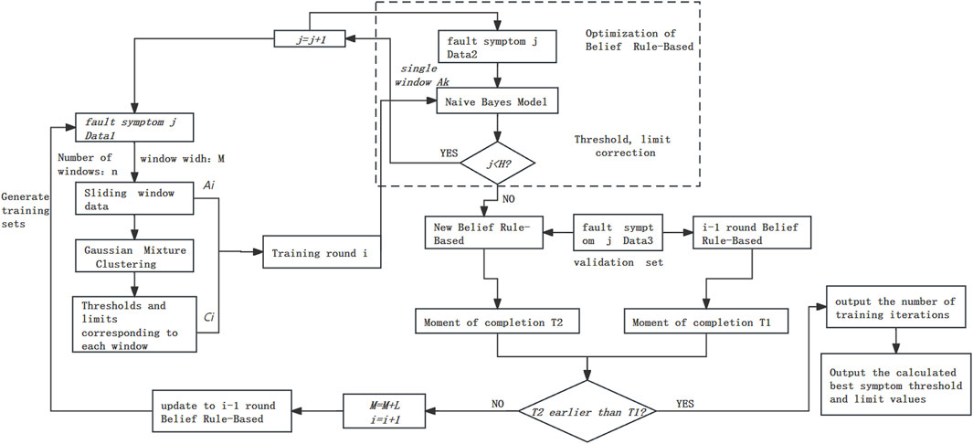
Figure 2. Flowchart of the belief rule-based iterative optimization.

4 Case study

In the instance verification of this paper, all program codes were executed in the same computing environment on a single computer. The specific hardware and software environments are presented in Table 1.

Table 1

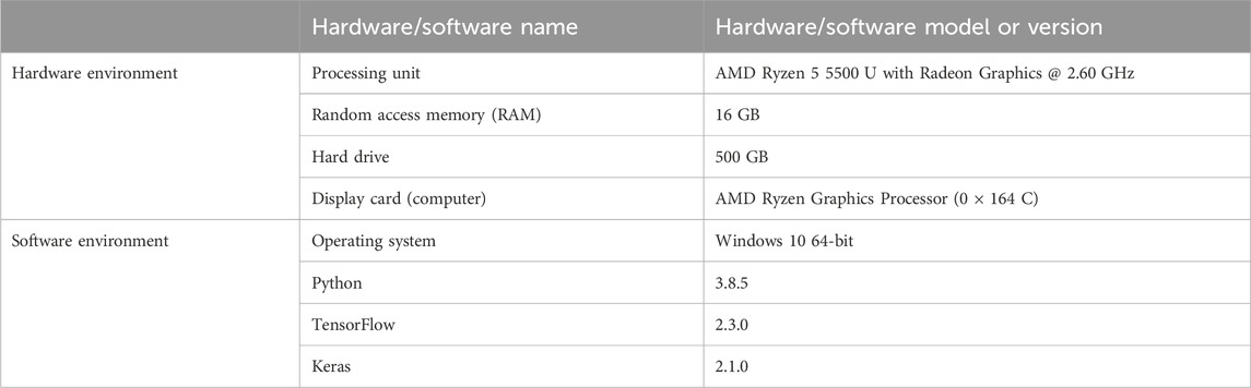
Table 1. Program hardware and software operating environment table.

First, using the established basic belief rule base for the heater, a fault diagnosis was conducted on the high-pressure heater and condenser of a 1000 MW nuclear power plant. All operational data were sampled at 1-min intervals. The diagnostic results showed the following results.

The condenser D experienced cooling water copper tube leakage faults on 16 November 2016, at 11:53 a.m.; 18 October 2017, at 10:35 a.m.; and 5 November 2019, at 12:21 p.m. The rule-matching degrees at these three time points were 0.3915, 0.3896, and 0.3976, respectively. The confidence levels for the conclusion of cooling water copper tube leakage faults were 0.8673, 0.8312, and 0.8532, respectively.

The condenser E experienced insufficient circulating water faults on 28 October 2019, at 07:34 a.m.; 6 January 2020, at 06:24 a.m.; and 31 May 2020, at 17:06 p.m. The rule-matching degrees at these three time points were 0.3532, 0.3815, and 0.3369, respectively. The confidence levels for the conclusion of insufficient circulating water faults were 0.7617, 0.8124, and 0.7993, respectively.

The high-pressure heater F experienced tubing leakage faults on 20 December 2016, at 09:56 a.m.; 10 September 2018, at 20:01 p.m.; and 18 November 2019, at 15:16 p.m. The rule-matching degrees at these three time points were 0.3677, 0.3922, and 0.3767, respectively. The confidence levels for the conclusion of the tubing leakage faults were 0.7916, 0.7896, and 0.8373, respectively.

The above diagnostic results are consistent with the provided information from the nuclear power plant, and all diagnostic results are correct. For ease of understanding, the faults diagnosed by the basic belief rule base for the condenser and high-pressure heater at different times are referred to as the first, second, and third faults.

Before training the model, the training dataset is first subjected to data cleaning, removing outliers and blank data. Subsequently, normalization is performed using Eq. 25. Data normalization not only enhances the convergence speed of the model but also improves the model’s accuracy to some extent. After testing, the test results are subjected to inverse normalization to output the actual data.

$X_{std}=\frac{X-X_{\mathit{min}}}{X_{\mathit{max}}-X_{\mathit{min}}}.(25)$

Here, x_std represents the normalized training dataset, x_min is the minimum value in the training dataset, and x_max is the maximum value in the training dataset.

To demonstrate the effectiveness of the improved method for calculating the optimal threshold and limit values in the belief rule base, a case study was conducted following the dataset partition shown in Table 2. The initial window width L was set to 60, and the increment in width M for each iteration was set to 60.

Table 2

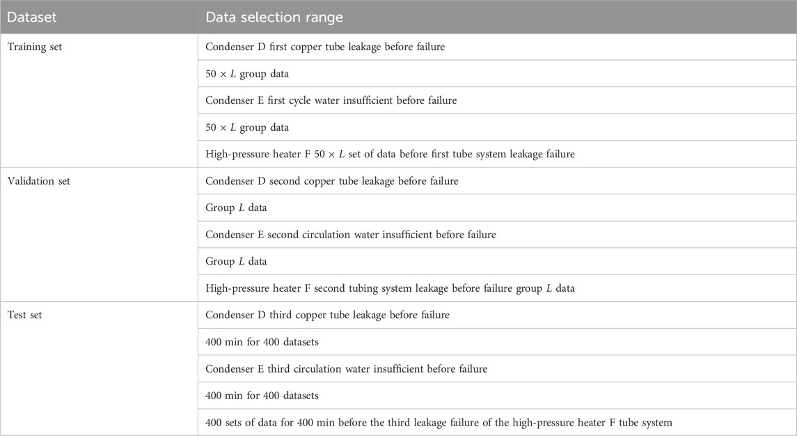
Table 2. Division of the dataset for the optimal threshold limit calculation methods.

Analyzing the dataset for condenser D, the improved model reached the constraint conditions after 11 training iterations. Using the improved belief rule base for the fault diagnosis of condenser D, a diagnosis of the third cooling water copper tube leakage fault for condenser D was made at 12:03 p.m. on 5 November 2019. The rule-matching degree and confidence level for the conclusion of a cooling water copper tube leakage fault at this time point were 0.3967 and 0.7965, respectively. Compared to the basic belief rule base, the diagnosis speed was improved by 18 min.

If diagnosing the third cooling water copper tube leakage fault for condenser D using the basic belief rule base, the confidence states of each fault symptom around that time point are illustrated in Figure 3. The red vertical dotted line corresponds to the moment when the improved belief rule base completes the diagnosis, and the orange vertical dotted line corresponds to the moment when the basic belief rule base completes the diagnosis. In the improved belief rule base, each fault symptom reaches the corresponding value in the confidence function defined by the optimal threshold and limit values faster than in the basic rule base. Therefore, the improved rule base has a faster diagnosis speed than the basic rule base.

Figure 3

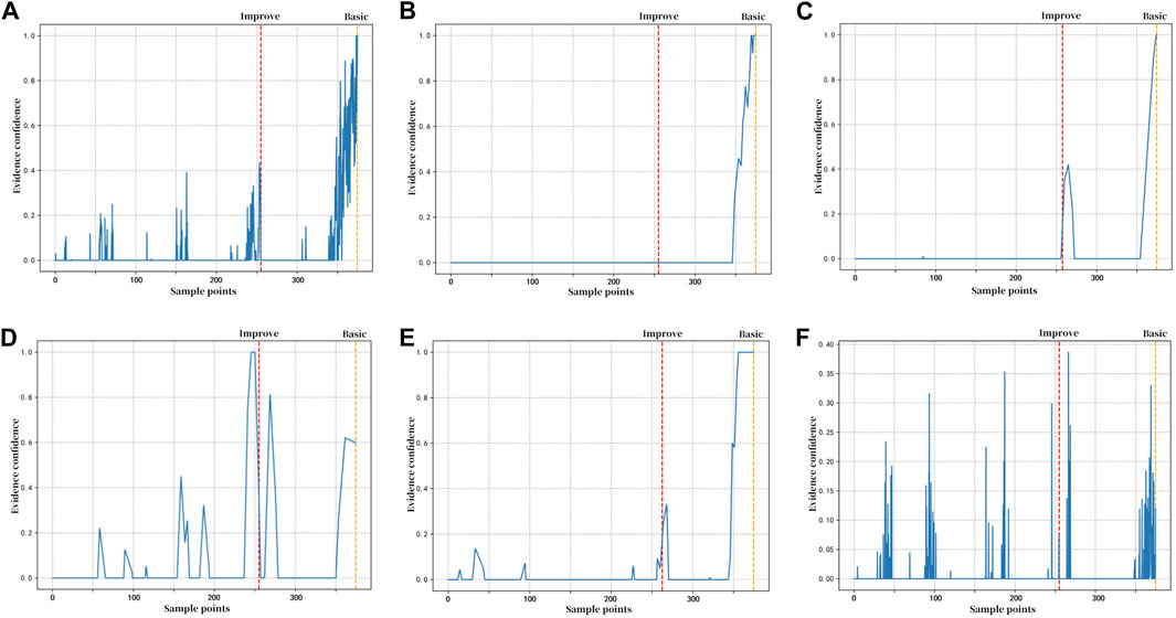
Figure 3. Evidence confidence of each fault symptom before condenser D third cooling water copper tube leakage failure. (A) Hot well water level; (B) vacuum level; (C) temperature difference; (D) condensate sub-cooling; (E) condensate pump motor current; and (F) condensate pump outlet pressure.

To more intuitively illustrate the advantages of the improved belief rule-based intelligent expert system, a comparative graph of the diagnostic results for the third cooling water copper tube leakage fault in condenser D of the nuclear power unit using both the basic and improved belief rule base is shown in Figure 4. In the figure, the red vertical dotted line corresponds to the moment when the improved belief rule base completes the diagnosis, and the orange vertical dotted line corresponds to the moment when the basic belief rule base completes the diagnosis.

Figure 4

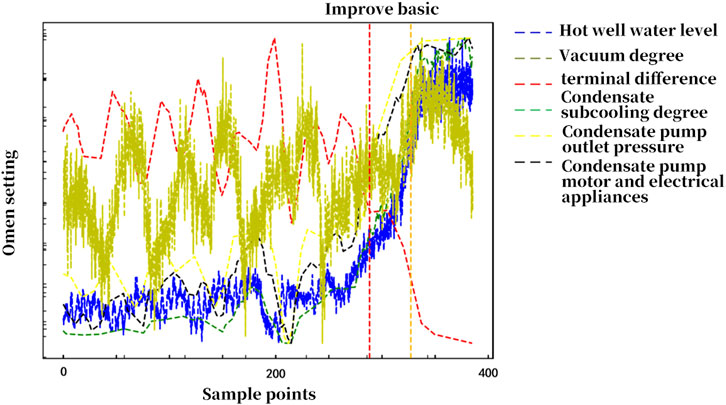
Figure 4. Comparative graph of diagnostic results for the second fault in condenser D using basic and improved belief rule bases.

To test the universality of the improved belief rule base proposed in this paper, the same experimental process was followed for the dataset of condenser E. The improved model reached the constraint conditions after nine training iterations. The results indicate that the improved belief rule-based model can complete the diagnosis for the third insufficient circulating water fault in condenser E at 16:51 on 31 May 2020. The comparative results with the basic belief rule base are shown in Figure 5. In the figure, the red vertical dotted line corresponds to the moment when the improved belief rule base completes the diagnosis, and the orange vertical dotted line corresponds to the moment when the basic belief rule base completes the diagnosis. For the second insufficient circulating water fault in condenser E, the improved belief rule base has a diagnosis speed improvement of 16 min compared to the basic belief rule base.

Figure 5

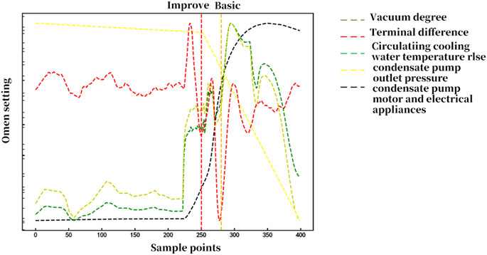
Figure 5. Comparative graph of diagnostic results for the third fault in condenser E using basic and improved belief rule bases.

Subsequently, the same experimental procedure was applied to analyze the dataset for high-pressure heater F. The improved model reached the constraint conditions after eight training iterations. It was found that the diagnosis of the third tube system leakage fault in heater F was completed at 15:01 on 18 November 2019. Compared to the basic belief rule base, the diagnosis speed was improved by 15 min. The comparative results of the two rule bases are shown in Figure 6. In the figure, the red vertical dotted line corresponds to the moment when the improved belief rule base completes the diagnosis, and the orange vertical dotted line represents the moment when the basic belief rule base completes the diagnosis.

Figure 6

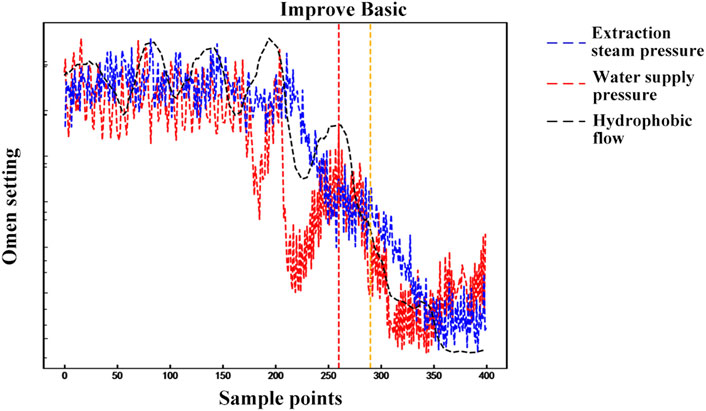
Figure 6. Comparative graph of diagnostic results for the third fault in high-pressure heater F using basic and improved belief rule bases.

5 Conclusion

In this paper, we conducted optimization research on belief rule bases using the Naive Bayes theory. Using Gaussian mixture clustering and Naive Bayes optimization, iteration is performed over the threshold and limit values of fault symptoms in the belief rule base, and we effectively addressed the timeliness and accuracy issues of a class of fault diagnoses with multiple fault symptoms related to multiple antecedent attribute differences. As historical fault samples accumulate, continuous iterative learning enhances the fit between the belief rule bases and real faults, promoting the speed of fault diagnosis. Diagnosing the cooling water copper tube leakage fault in condenser D using an improved belief rule-based approach resulted in an 18-min improvement in diagnostic speed compared to a basic belief rule-based approach. This approach has a certain reference value for fault rule-based diagnosis in process industries.

This optimization of the belief rule-based approach is researched based on the premise of certain membership functions. Further research could consider optimizing the membership functions. Additionally, fast convergence problems in fault diagnosis processes require further research.

Data availability statement

The original contributions presented in the study are included in the article/Supplementary Material; further inquiries can be directed to the corresponding author.

Author contributions

HQ: formal analysis, validation, and writing–review and editing. YP: investigation, software, and writing–original draft. XW: visualization and writing–review and editing. ZL: supervision and writing–review and editing.

Funding

The author(s) declare that financial support was received for the research, authorship, and/or publication of this article. This research was funded by the Nation Natural Science Foundation of Shanghai (Research on Uncertainty Reasoning and Correlation Mechanism in Nuclear Power Risk Assessment), grant number 192R1420700.

Acknowledgments

The authors thank the Shanghai Key Laboratory of Power Station Automation Technology for providing experimental facilities.

Conflict of interest

Authors XW and ZL were employed by China Nuclear Power Engineering Co., Ltd.

The remaining authors declare that the research was conducted in the absence of any commercial or financial relationships that could be construed as a potential conflict of interest.

Publisher’s note

All claims expressed in this article are solely those of the authors and do not necessarily represent those of their affiliated organizations, or those of the publisher, the editors, and the reviewers. Any product that may be evaluated in this article, or claim that may be made by its manufacturer, is not guaranteed or endorsed by the publisher.

References

Ahmed, F., Chakma, R. J., Hossain, S., and Sarma, D. (2020). “A combined belief rule based expert system to predict coronary artery disease,” in Proceedings of the 2020 International Conference on Inventive Computation Technologies (ICICT), Coimbatore, India, 26–28 February 2020, 252–257.

CrossRef Full Text | Google Scholar

Chen, Q., Qian, H., and Zhang, L. (2018). Research on soot blowing diagnostic method of boiler heating surface based on evidence fusion. J. Electr. Power Sci. Technol. 33 (3), 6. (In Chinese). doi:10.3969/j.issn.1673-9140.2018.03.021

CrossRef Full Text | Google Scholar

Frank, E., Hall, M., and Pfahringer, B. (2002). “Locally weighted navie Bayes,” in Proceedings of the Nineteenth Conference on Uncertainty in Artificial Intelligence, Acapulco, Mexico, 1–5 August 2002, 249–256.

Google Scholar

Gao, M., Chen, C., Shi, J., Lai, C. S., Yang, Y., and Dong, Z. (2020). A multiscale recognition method for the optimization of traffic signs using GMM and category quality focal loss. Sensors 20 (17), 4850. doi:10.3390/s20174850

PubMed Abstract | CrossRef Full Text | Google Scholar

Li, X., Yang, Y., and Xu, Y. (2020). Detection of moving targets by four-frame difference and modified Gaussian mixture model. Sci. Technol. Eng. 20 (15), 6141–6150. (In Chinese). doi:10.3969/j.issn.1671-1815.2020.15.037

CrossRef Full Text | Google Scholar

Lv, M., and Sun, J. (2019). Moving image target detection based on modified Gaussian mixture model. Semicond. Optoelectron. 40 (6), 874–878. (In Chinese). doi:10.16818/j.issn1001-5868.2019.06.026

CrossRef Full Text | Google Scholar

McLachlan, G. J., and Basford, K. E. (1988). Mixture models: inference and applications to clustering. New York, USA: Marcel Dekker.

Google Scholar

Pearl, J. (1988). Probabilistic reasoning in intelligent systems: Networks of plausible inference. Palo Alto, USA: Morgan Kaufmann Publishers. doi:10.1016/C2009-0-27609-4

CrossRef Full Text | Google Scholar

Wolfe, J. H. (1963). Object cluster analysis of social areas. Berkeley: University of California. BS thesis.

Google Scholar

Xiao, H., Li, Y., and Lv, Y. (2011). Gear fault recognition based on recurrence quantification analysis and Gaussian mixture model. J. Vibr. Eng. 24 (1), 84–88. (In Chinese). doi:10.3969/j.issn.1004-4523.2011.01.015

CrossRef Full Text | Google Scholar

Yang, J. B., Liu, J., Wang, J., Sii, H. S., and Wang, H. W. (2006). Belief rule-base inference methodology using the evidential reasoning Approach-RIMER. IEEE Trans. Syst. Man. Cybern. Part A Syst. Humans 36 (2), 266–285. doi:10.1109/TSMCA.2005.851270

CrossRef Full Text | Google Scholar

Zhang, C., and Guo, M. (2015). Research and realization of improved native Bayes classification algorithm under big data environment. J. Beijing Jiaot. Univ. 39 (2), 35–41. (In Chinese). doi:10.11860/j.issn.1673-0291.2015.02.006

CrossRef Full Text | Google Scholar

Zheng, M., Qian, H., Lin, S., Xiao, B., Chu, X., Fei, M., et al. (2018). Research on knowledge base of intelligent diagnosis expert based on tubing leakage of high-pressure heater in nuclear power plants. Nucl. Power Eng. 39 (1), 146–151. (In Chinese). doi:10.13832/j.jnpe.2018.01.0146

CrossRef Full Text | Google Scholar