Spatially-explicit estimation of Wright's neighborhood size in continuous populations

Introduction

Populations lose allelic diversity and heterozygosity through the processes of genetic drift and inbreeding, respectively (Amos and Harwood, 1998). If this diversity is not replaced by the processes of mutation and immigration, the population loses alleles and heterozygosity at a rate proportional to the number of breeding individuals (Wright, 1931). Diminished genetic diversity may reduce a population's capacity for adaptation in dynamic environments (though dominance, epistasis, and pleiotropy may strongly affect this relationship; Reed and Frankham, 2001), lower the frequency of heterozygotes (and therefore the prevalence of heterozygote vigor or heterosis), favor inbreeding depression, and ultimately increase the risk of extinction (Frankham et al., 2002).

Wright (1931) first defined the concept of effective population size (N_e) as the number of breeding individuals in an ideal population experiencing the same rate of drift as the real population of interest. Factors like unequal sex ratios, a fluctuating population size, overlapping generations, high variability in the distribution of offspring, and non-random mating make the effective size of a population lower than the census size (N_c) because they influence the number of individuals that contribute their genetic variation to the next generation (Frankham et al., 2002). Therefore, the risk of extinction posed by reduced genetic diversity is more closely related to N_e than N_c, making N_e is an important parameter in conservation genetics (Lande and Barrowclough, 1987).

N_e may be calculated from demographic data (Caballero, 1994; Wang and Caballero, 1999) that are often difficult to acquire from wild populations. Instead, N_e is more commonly estimated from genetic data. Long-term genetic estimates of N_e may be obtained from the relationship between genetic diversity (θ) and the mutation rate (μ):

$\theta =4N_e\mu$

Alternatively, short-term genetic estimates of N_e may be derived from genetic data sampled from one or more recent generations. Single-sample methods reflect the effective number of breeding individuals (N_b) in the sampled generation, and have been based on rates of drift or inbreeding from heterozygote excess (Pudovkin et al., 1996), linkage disequilibrium (Hill, 1981), and molecular co-ancestry (Wang, 2009). A two-sample temporal method (Waples, 1989) estimates the harmonic mean of N_e from genetic drift that occurs over the time between samples, but when sampling intervals are from recent generations, it is also a contemporary measure of N_e. These contemporary estimates of N_e differ from Wright's original concept of N_e, which reflects the long-term harmonic mean number of effective breeding individuals over many generations.

Wright's original concept of N_e assumes a closed panmictic population. In many wild populations, however, individuals are continuously distributed across a landscape, and mating probabilities are a function of Euclidean distance (i.e., isolation by distance or IBD; Wright, 1943) or effective distance given the variable resistance of the landscape to gene flow (i.e., isolation by resistance or IBR; McRae, 2006). Such populations become internally structured into continuously overlapping local neighborhoods of breeding individuals. To quantify N_e in continuous populations isolated by distance, Wright proposed the concept of a genetic neighborhood (Wright, 1946), defined as

$NS=4\pi {\sigma }^{2}D$

where NS is the number of breeding individuals in the local neighborhood, σ is the mean squared parent-offspring dispersal distance along one axis in a two-dimensional habitat (assuming a Gaussian dispersal function), and D is the ideal population density (i.e., the number of ideal individuals per unit area). A genetic neighborhood under isolation by distance forms a circle with a radius of 2σ, reflecting the local area within which gene flow is high relative to drift (i.e., the neighborhood, rather than the global population, approaches panmixia).

Maruyama (1972) demonstrated that if the local extent of breeding is small relative to the global population, σ²D < 1 and genetic diversity is lost from the global population at a rate approximated by σ²D/(2N) per generation. Conversely, when the local extent of breeding is large and approaches the global population, σ²D > 1 and genetic diversity declines at approximately the same rate as a panmictic population (i.e., 1/2N per generation). Thus, in continuous populations highly structured by distance or patterns of resistance, the capacity to retain genetic diversity is driven by the local NS rather than the global effective size.

Methods have been developed to infer NS based on the approximately linear relationship expected between the logarithm of spatial distance and genetic distances among individuals (e.g., Rousset, 2000; Hardy and Vekemans, 2002; Rousset and Leblois, 2011). For diploid individuals in a two-dimensional habitat, NS is equal to 1 divided by the slope of the regression between individual genetic distance and the log of distance (Rousset, 2000). Importantly, estimating NS using this approach, or from demographic estimates of σ²D, provides a single estimate of the local NS for the entire population, assuming no spatial variation in NS.

In the center of a uniformly distributed population isolated by distance, effective population density and neighborhood area are constant, and there is no expectation for spatial variation in NS. However, for genetic neighborhoods near the population's periphery, the edge would be expected to reduce the neighborhood's area, resulting in a lower NS, and giving rise to spatial heterogeneity in NS. Similarly, spatial variation in effective population density (D) would also be expected to produce spatial variation in NS. Furthermore, in populations inhabiting heterogeneous landscapes (i.e., isolation by resistance), patterns of resistance may create variability in the area of genetic neighborhoods and thereby produce spatial variation in NS.

To date, attempts to quantify NS in continuous populations have not addressed the potential for spatial variation in NS. Yet spatial genetic variation in genetic processes is an inherent property of populations isolated by distance or resistance (Rohlf and Schnell, 1971; Ibrahim et al., 1996; Miller, 2005; Shirk and Cushman, 2011). Failure to detect this variation could lead to incorrect inferences regarding the true range of NS across a study area and potentially misinform conservation efforts, particularly near the periphery or in areas where patterns of resistance or population density differ strongly from the rest of the population. Indeed, all wild populations have edges, and they are often of particular interest in conservation genetics (García-Ramos and Kirkpatrick, 1997). A means of detecting spatial variation in NS that provides unbiased estimates even near a population's periphery is needed.

Detecting spatial variation in NS for populations isolated by resistance or distance requires a means to produce estimates of NS across the population at multiple locations or as a continuous surface while accounting for the continuous nature of the population. We previously described an approach (Shirk and Cushman, 2011) to estimate genetic diversity indices spatially using Wright's concept of a genetic neighborhood. The outer extent of Wright's neighborhood in a continuous population isolated by distance is a circle with a radius of 2σ. By placing this circular neighborhood around each sampled individual, and estimating genetic diversity indices from all individuals within the circle, we matched the sampling unit to the local breeding extent. This produced a spatially explicit estimate of genetic diversity that was not biased by a Wahlund effect (Wahlund, 1928) that occurs when calculating genetic indices at broad extents relative to the local population structure. These analysis extents overlapped in space such that an individual could belong to multiple neighborhoods, reflecting the continuous nature of the population.

In addition to offering a spatially explicit and unbiased means of estimating genetic diversity indices, in Shirk and Cushman (2011), we extended Wright's neighborhood concept to also include populations fitting the IBR model by defining neighborhoods in terms of effective rather than Euclidean distances (e.g., based on cost-weighted distances given a raster model of landscape resistance to gene flow). With this approach, the neighborhood extent is an irregularly shaped kernel rather than a circle (as is the case in an IBD population neighborhood; Figure 1). Whether the neighborhood is a circle or a kernel, the outer edge is 2σ from the center. If NS were estimated locally in analysis neighborhoods centered on each sampled individual in the population, it would provide a means to detect spatial variation in NS in continuous populations isolated by distance or resistance.

FIGURE 1

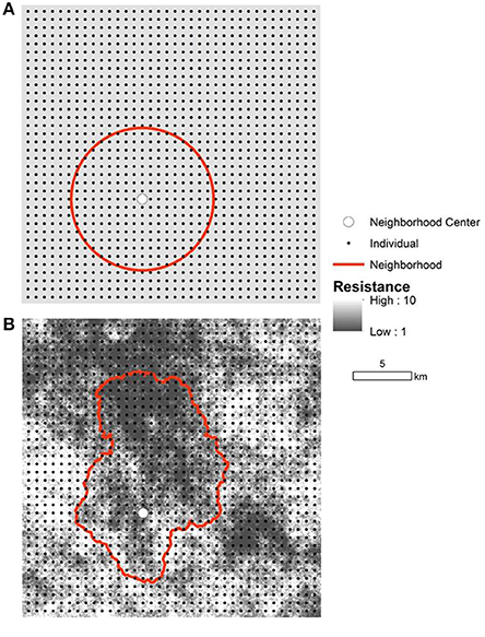
Figure 1. Simulated landscapes, populations, and neighborhoods. The isolation by distance population (IBD; A) and the isolation by resistance population (IBR; B) consisted of 1296 individuals (black dot) arrayed in a 36 × 36 regular grid. Mating and dispersal probabilities in the simulation were probabilistic functions of the Euclidean distance or effective distance between individuals in the IBD and IBR simulations, respectively. Effective distances were based on cost-weighted distances given a raster model of resistance to gene flow (example in B). Resistance varied from 1 (black) to 10 (white) and the spatial pattern differed between replicate IBR simulations. The square landscapes measured 25.6 km per side. An example of the extent of Wright's genetic neighborhood is shown in each panel (red line) for a single individual at the center (large white circle).

Because analysis neighborhoods are defined by a radius of 2σ, σ is a critical parameter. Yet for most species, mean squared parent-offspring dispersal distances are not known and difficult to estimate from field data. Importantly, Neel et al. (2013) found strong bias in the estimate of NS based on the linkage disequilibrium (LD) method when the sampling extent over which NS was calculated did not match the local breeding extent (2σ). Furthermore, they reasoned that a positive or negative inbreeding coefficient (F_IS) would be apparent if the sampling extent was larger or smaller than the extent of local breeding, respectively. Iteratively exploring a range of neighborhood extents until F_IS approached zero could therefore be used to identify Wright's neighborhood extent (2σ). If this or other approaches based on genetic data were to reliably identify the appropriate analysis extent, it would allow for unbiased estimates of NS in continuous populations without requiring the difficult task of inferring σ from field data.

In this study, we used an approach analogous to Shirk and Cushman (2011) to assess spatial variation in NS in both simulated IBD and IBR populations and a real population of mountain goats (Oreamnos americanus) inhabiting a complex landscape. Based on these simulations, we explored several questions. First, we evaluated the ability of our spatially-explicit implementation of Wright's neighborhood concept to accurately estimate NS in populations isolated by distance or resistance without bias. Second, we evaluated two approaches to inferring σ from the same genetic data used to estimate NS. Third, we examined whether proximity to the population edge produced bias in the estimate of NS. Lastly, we explored spatial variation in NS in the simulated IBD and IBR populations as a real population of mountain goats. We expected estimates of NS to be unbiased as long as the radius of the neighborhood was equal to 2σ. We also expected strong spatial variation in NS within the IBD, IBR, and mountain goat populations, and that peripheral areas or regions isolated by strong patterns of resistance would have the lower NS relative to the population core.

Materials and Methods

Simulated Populations, Landscapes, and Distances

We simulated mating and dispersal in continuous populations isolated by distance (IBD) or resistance (IBR). Each simulation was replicated 100 times. In all simulations, the landscape was represented by a square 256 × 256 cell raster grid with square cells measuring 100 m per side. The populations were constant in size (N = 1296) and distribution (a 36 × 36 uniform square grid with 700 m between individuals), however, the IBD and IBR landscapes differed in their capacity to limit the movement of mating and dispersing individuals. In the IBD population, mating and dispersal probabilities were based on the Euclidean distance between individuals. Because the population size and distribution was constant in all simulations, the Euclidean distance between individuals was constant in the IBD populations. In the IBR populations, however, mating and dispersal probabilities were a function of the Euclidean distance weighted by the landscape's resistance to gene flow (i.e., the effective or cost-weighted distance).

We used the program QRULE (Gardner, 1999) to create the IBR landscapes, with resistance values ranging from 1 to 10 in equal area proportions. These values represented resistance to movement such that the “cost” to traverse a grid cell was equal to the cell size (100 m) times the resistance. Thus, a value of one implies that the Euclidean and effective distances are equal. A population isolated by distance can be thought of as inhabiting a raster landscape with a resistance of one in all cells. Values greater than one indicate additional cost to movement beyond the effect of distance alone (e.g., suboptimal habitat types). Resistance values were spatially distributed with a QRULE H parameter value of 0.1, which produced clumped distributions that are commonly observed in real landscapes (Figure 1). Because this pattern of resistance varied between replicate runs, the effective distance between individuals varied among the IBR simulations.

Mating and dispersal probabilities in the simulations were based on the Euclidean (for the IBD population) or effective (for the IBR population) distances between individuals. We calculated pairwise Euclidean distances in an N × N matrix (N = 1296) using the Ecodist package (Goslee and Urban, 2007) in R (R Development Core Team, 2013). We calculated effective distances with the gdistance package (van Etten, 2011) in R based on the cumulative cost of the least-cost path given the raster model of landscape resistance for each IBR simulation replicate.

Population Genetic Simulations

We used the population genetic simulation software CDPOP (Landguth and Cushman, 2010) to simulate mating and dispersal in IBD and IBR populations (100 replicates each). CDPOP is an individual-based simulator of population genetic processes. It simulates mating and dispersal in a finite population assigned to fixed locations. Over a user-specified number of generations, CDPOP records allele usage by all individuals per generation, and computes various population genetic statistics. In each generation, adult individuals mate according to a user-specified mating system and probability function based on proximity in Euclidean or effective distance. Once mated, females give birth to a number of offspring determined by a user-specified probability function which can also control the sex ratio at birth. After birth, adult mortality occurs probabilistically based on user-specified demographic information. Finally, vacant locations where adults have died are filled by dispersing offspring. Dispersal probabilities follow a user-specified function based on Euclidean or effective distances to the vacant locations. If all locations are occupied, any remaining offspring not yet assigned to a location are eliminated. Unoccupied sites may be filled by immigrants or left open.

We parameterized the IBD and IBR CDPOP simulations to reflect a hermaphroditic animal distributed at a moderate uniform density with limited movement capability relative to the size of the landscape, thus allowing for spatial patterns in effective population size to emerge over time. Parameters matched the assumptions of an ideal Wright-Fisher population and Wright's genetic neighborhood. Thus, the census number of individuals within a genetic neighborhood was equal to effective number of breeding individuals, allowing for genetic estimates of NS to be related to the true NS. We specified mating and dispersal probabilities to be a Gaussian function of Euclidean or effective distance (for the IBD and IBR populations, respectively), with a maximum equal to 30% of the landscape width (7680 m in Euclidean units). Except for varying mating and dispersal probability as a function of the landscape, the CDPOP parameters were the same in all simulations. Generations were discrete and non-overlapping. There was no selection, mutation, or immigration from outside the population. Individuals were diploid. Mating was sexual (equivalent to hermaphroditic with selfing not allowed). The number of offspring was based on a Poisson distribution with a mean of 4, providing ample offspring to fill all vacant locations. The simulation tracked alleles at 20 loci, with 20 alleles randomly assigned per locus to the first generation. At the end of 300 generations, CDPOP recorded the genotypes of all individuals in the population.

Empirical Landscape and Genetic Data

To explore spatial variation in the NS of a real population, we used genetic data previously collected (Shirk et al., 2010) from mountain goats in the Cascade Range in Washington State (USA). The majority of the area is encompassed by national forests and national parks. The landscape is mountainous and covered with montane forests, except at elevations above about 1400 m, where subalpine parkland, rocky alpine summits, and glaciers predominate. Elevation varies from near sea level to almost 4400 m. One major interstate highway, several state highways, and a network of logging roads extend throughout the study area.

We previously genotyped 135 mountain goats sampled from this region at 18 microsatellite loci (Shirk et al., 2010). These genotypes were used to calculate pairwise inter-individual genetic distances, which we related to effective distances (based on various resistance hypotheses) in a causal modeling framework (Cushman et al., 2006; Shirk et al., 2010). This identified a model of landscape resistance as causal relative to alternative resistance models or null models of isolation by distance or barriers. The causal model accounted for the influence of elevation, land cover, and roads on gene flow. In the present analysis, we used this resistance model to define genetic neighborhoods for mountain goats within the study area, and the genotypes to estimate NS within the neighborhoods.

Inferring σ from Genetic Data

We evaluated two approaches to using genetic data to infer the mean squared parent-offspring dispersal distance (σ) that determines the spatial extent of Wright's neighborhood. We used the program sGD (Shirk and Cushman, 2011) to calculate the inbreeding coefficient (F_IS) and a chi-square test for goodness-of-fit to Hardy-Weinberg equilibrium (HWE) within genetic neighborhoods centered on each individual's location in the IBD and IBR simulated populations. The outer extent of each neighborhood was defined in terms of σ, which was recorded by CDPOP during the simulations. Because of the Wahlund effect that occurs when the analysis extent does not match Wright's genetic neighborhood (Neel et al., 2013), we expected F_IS to be positive and the HWE test p-value to be significant (α = 0.05; the null hypothesis was that the sample was in HWE) when the analysis extent was > 2σ. Conversely, when the analysis extent was < 2σ, we expected F_IS to be negative and the HWE test p-value to not be significant. To quantify bias and error when σ was not known, we estimated σ by iteratively increasing the analysis neighborhood from 5 to 50% of the Euclidean or effective distance (for the IBD and IBR simulations, respectively) to cross the landscape, in 5% increments. The estimated σ was defined by the distance at which F_IS was closest to zero or the HWE test p-value was closest to 0.05.

Estimating NS

To estimate NS spatially, we modified the previously described program sGD (Shirk and Cushman, 2011), which calculates genetic diversity indices within genetic neighborhoods given a spatially referenced set of co-dominant input genotypes and a matrix of pairwise inter-individual landscape distances. Distances may be calculated in Euclidean or effective units as appropriate for the landscape and population of interest. For each genotyped individual in the sample, sGD uses the distance matrix to identify all other individuals that are below a user specified threshold distance (i.e., the neighborhood radius). Genetic diversity indices are then calculated from the genotypes of all individuals within each neighborhood. For this analysis, we modified sGD to also estimate NS within the same genetic neighborhoods via a dependency on the program NeEstimator (Do et al., 2014). NeEstimator implements the most widely used one-sample estimator, the Burrow's method based on linkage disequilibrium (LD) resulting from genetic drift in a finite population (Cockerham and Weir, 1977; Hill, 1981; Weir, 1996). The LD method estimates the number of breeding individuals responsible for the sample (N_b), for the parental generation (Hill, 1981; Waples, 2006; Waples and Do, 2008). The method to estimate NS spatially (as well as the original methods to estimate common indices of genetic diversity) is now implemented in the sGD package in R (R Development Core Team, 2013).

For each replicate in the IBD and IBR simulations, we used the sGD package to estimate NS within genetic neighborhoods centered on each of the 1296 individuals in the population. The radius of the neighborhood was determined by the mean squared parent-offspring dispersal distance (σ), which was recorded by CDPOP during the simulations. We varied this extent from 1 to 4σ, using Euclidean distances for the IBD populations and effective distances for the IBR populations (calculated as described above). These pairwise distances defining the genetic neighborhoods were the same distances that determined mating and dispersal probabilities in the CDPOP simulations. After 300 simulated generations, we used the sGD package to calculate ${\widehat{N}}_b$ within neighborhoods with at least 20 individuals (to reduce error from small sample sizes). To limit bias due to inclusion of rare alleles, we included only alleles with a frequency > 0.01 (Waples and Do, 2010). Because our simulation parameters met the Wright-Fisher assumptions of an ideal population, the number of individuals in each genetic neighborhood of radius 2σ was equal to the NS based on Wright's definition. This provided a means to compare ${\widehat{N}}_b$ to the true NS. We also used the sGD package to estimate NS spatially from the mountain goat genotypes, resistance model, and estimate of σ described above and published in Shirk et al. (2010).

Results

In the CDPOP simulations, the lack of mutation and immigration allowed drift and inbreeding to reduce allelic diversity and heterozygosity in the population over time (Figure 2). Observed heterozygosity (H_o) was lower than expected heterozygosity (H_e), resulting in a positive inbreeding coefficient (F_IS). This reflects a Wahlund effect due to substructure within the sampling extent (i.e., the entire population). The population was more highly structured in the IBR simulation compared to the IBD simulation, and inbreeding was correspondingly higher. That inbreeding plateaued after 20–30 generations indicates population genetic structure formed very rapidly, and was stable for the remainder of the simulation.

FIGURE 2

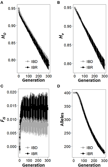
Figure 2. Change in population genetic indices over 300 simulated generations. Observed heterozygosity (H_o; A), expected heterozygosity (H_e; B), inbreeding coefficient (F_IS; C), and the number of alleles (A; D) in the population were recorded for each generation, for both the isolation by distance (IBD; gray line) and isolation by resistance (IBR; black line) simulations. Each plot represents the mean and standard deviation of 100 replicate simulations.

In the IBD simulations, mean σ across 100 replicates was 3058 m (SD 82 m) in Euclidean distance units. In the IBR simulations, mean σ was 10950 m (SD 650 m) in effective distance units. As the analysis neighborhood radius was increased from 1 to 4σ, the number of individuals in the neighborhood (N) and the estimate of NS (${\widehat{N}}_b$) increased (Figures 3A,B, respectively). In both the IBD and IBR simulations, the mean ${\widehat{N}}_b$:NS ratio for all neighborhoods approached 1 only when the analysis extent radius was 2σ (Figure 3C). Thus, ${\widehat{N}}_b$ was not biased when the analysis extent matched the extent of Wright's genetic neighborhood. However, at analysis extents < 2σ, ${\widehat{N}}_b$:NS was > 1, indicating bias toward overestimation. Conversely, at analysis extents > 2σ, ${\widehat{N}}_b$:NS was < 1, indicating a bias toward underestimation.

FIGURE 3

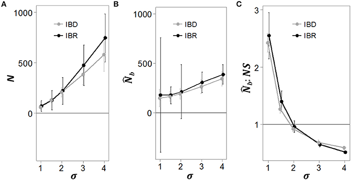
Figure 3. Bias in the estimate of NS as a function of the analysis window extent. Simulated genotypes at generation 300 were grouped into overlapping analysis neighborhoods of varying extents. The analysis extents were defined in terms of σ, the mean squared parent-offspring dispersal distance recorded during the simulations. In (A), the number of individuals per neighborhood at each analysis extent is shown for both the isolation by distance (IBD; gray line) and isolation by resistance (IBR) simulations. In (B), ${\widehat{N}}_b$ (the estimated number of breeding individuals responsible for the sample) calculated using the LD method (implemented in the program NeEstimator) at varying analysis neighborhood extents is shown. We used ${\widehat{N}}_b$ as an estimate of Wright's neighborhood size (NS; the actual number of breeding individuals in a neighborhood with a radius of 2σ). Bias in this estimate at analysis neighborhood extents that do not match the extent of local breeding becomes apparent when the ratio of ${\widehat{N}}_b$:NS is < or > 1.0 (C). Each plot represents the mean and standard deviation of 100 replicated simulations.

As the analysis neighborhood increased in radius from 1 to 4σ, the mean F_IS within neighborhoods in the IBD and IBR populations transitioned from negative to positive values at 2σ, though the variance across replicate runs was high (Figure 4A). Similarly, a chi-square test for HWE within each neighborhood became significant at α = 0.05 when the analysis neighborhood approached 2σ, though we observed high variability across replicate runs (Figure 4B). Using the above relationships to infer σ by iteratively increasing the analysis neighborhood, we found the point at which the HWE test p-value became significant was often less than σ. Estimating NS using this biased estimate of σ to define the analysis neighborhoods added considerable error and a strong bias toward overestimating NS, in both the IBD and IBR populations (Table 1). The distance at which F_IS transitions from negative to positive produced highly variable estimates of σ, which when used as the analysis neighborhood also added considerable error to the estimate of NS, but no strong bias (Table 1).

FIGURE 4

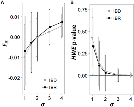
Figure 4. F_IS and HWE test p-value as a function of the analysis window extent. Simulated genotypes after 300 generations were grouped into overlapping analysis neighborhoods of varying extents. The analysis extents were defined in terms of σ, the mean squared parent-offspring dispersal distance recorded during the simulations. The inbreeding coefficient (F_IS; A) and the p-value for a chi-square test of Hardy-Weinberg equilibrium (HWE; B) were calculated for each analysis neighborhood extent in both the isolation by distance (IBD; gray lines) and isolation by resistance (IBR; black lines) simulations. Each plot represents the mean and standard deviation of 100 replicated simulations.

TABLE 1

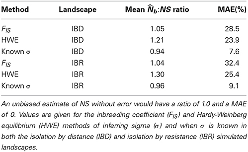
Table 1. Mean ratio of ${\widehat{N}}_b$ (the estimated number of breeding individuals in the neighborhood sample) to NS (the true neighborhood size), and mean absolute error (MAE; as a percent of the true neighborhood size) in the estimate of NS, over 100 replicate simulations.

When the analysis extent matched the extent of breeding at a radius of 2σ, the distribution of ${\widehat{N}}_b$:NS ratios was approximately centered on 1 in neighborhoods at varying distances from the edge, in both the IBD and IBR populations (Figure 5), indicating no bias in the estimate of NS due to edge effects. Furthermore, spatial variation in NS was highly apparent in all simulations. In the IBD simulations, the mean NS across all simulations was highest in the center of the landscape and decreased uniformly toward the periphery (Figure 6A). In the IBR simulations, NS also tended to be higher in the center of the landscape relative to the periphery (Figure 6B). However, the complex pattern of resistance created complex patterns in NS that varied between each simulated IBR landscape. Spatial variation in NS was also strong in a population of mountain goats in the Cascade Range, Washington, USA (Figure 7). The southern part of the population, which has a high local density of individuals, had the largest relative NS whereas in the north, where mountain goats are sparsely distributed, NS was comparatively low.

FIGURE 5

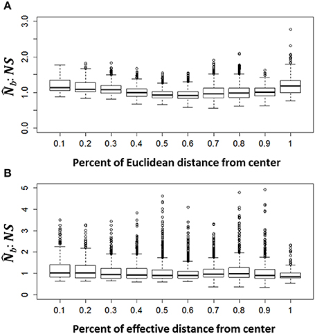
Figure 5. Spatial variation in ${\widehat{N}}_b$. The number of breeding individuals responsible for the sample (${\widehat{N}}_b$) was calculated within genetic neighborhoods with a radius of 2σ (the mean squared parent-offspring dispersal distance) in both the isolation by distance (IBD; A) and isolation by resistance (IBR; B) simulations after 300 generations. In (A), the mean ${\widehat{N}}_b$ of 100 replicate simulations is shown. In (B), one example from the 100 replicate simulations is shown, because neighborhood extents varied between replicates in the IBR simulations.

FIGURE 6

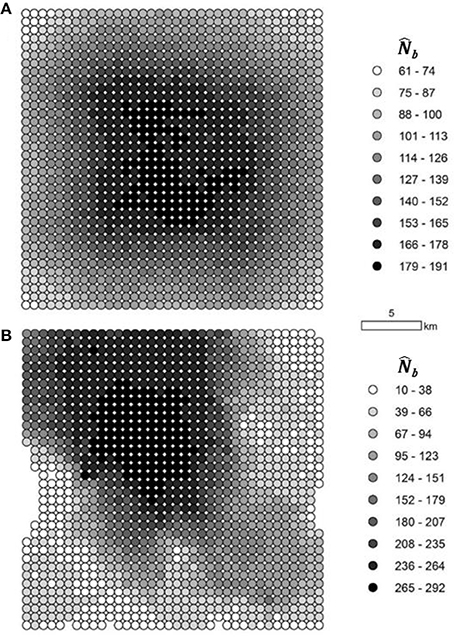
Figure 6. Edge bias in ${\widehat{N}}_b$. Simulated genotypes after 300 generations were grouped into overlapping analysis neighborhoods with a radius of twice the mean squared parent-offspring dispersal distance (σ) recorded during the simulations, for both the isolation by distance (IBD; A) and isolation by resistance (IBR; B) populations. ${\widehat{N}}_b$ (the estimated number of breeding individuals responsible for the sample) was calculated for each neighborhood using the LD method (implemented in the program NeEstimator). We used ${\widehat{N}}_b$ as an estimate of Wright's neighborhood size (NS; the actual number of breeding individuals in a neighborhood with a radius of 2σ). Bias in the estimate of NS at varying percent distances from the center of the population would be evident if the ratio of ${\widehat{N}}_b$:NS is < or > 1.0 (C). The dark horizontal line in each boxplot represents in median ratio of all neigborhodos and the top and bottom of the box depict the 25th and 75th percentile of ratios. The whiskers extend to the smallest and largest values in the data that are not outliers (open circles). Each plot summarizes 100 replicate simulations.

FIGURE 7

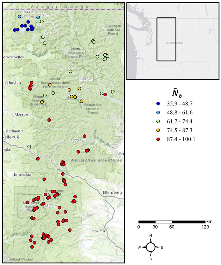
Figure 7. Spatial variation in mountain goat ${\widehat{N}}_b$. Genotypes sampled from a population of mountain goats inhabiting the Cascade Range, Washington, USA were grouped into overlapping neighborhoods based on effective distances calculated from an empirical resistance model and a radius defined by twice the estimated mean squared parent-offspring dispersal distance (σ). The estimated number of breeding individuals responsible for the sample (${\widehat{N}}_b$) was calculated for each neighborhood using the LD method (implemented in the program NeEstimator). Warm colors indicate higher relative ${\widehat{N}}_b$ and cool colors represent lower relative ${\widehat{N}}_b$.

Discussion

Spatial genetic variation is an expected property of continuous populations when the extent of the population exceeds the local extent of dispersal and mating (Ibrahim et al., 1996; Miller, 2005; Shirk and Cushman, 2011). In this study, we describe an application of Wright's neighborhood concept designed to quantify spatial variation in NS for continuous populations isolated by distance or resistance. We previously applied this method to estimating spatially-explicit indices of genetic diversity in Shirk and Cushman (2011). Here, we extend this approach to also estimate NS in local analysis neighborhoods surrounding each sample location. Matching the analysis neighborhood to the local extent of breeding in the population provided unbiased estimates even near the periphery of a population, and revealed complex patterns of NS that have important conservation implications for continuous populations.

Neel et al. (2013) applied a similar approach to estimate NS in local neighborhoods, but not in a spatially-explicit manner and only for populations isolated by distance. There were also differences between these studies in terms of how genetic neighborhoods were defined and simulated. Wright's neighborhood assumes a Gaussian dispersal function and an outer extent that is a circle with a radius of 2σ. This extent contains about 87% of the potential parents for an individual at the center. In Neel et al. (2013), the genetic neighborhood was a square containing 100% of potential parents and the distances between parents and offspring followed a uniform distribution. In the present analysis, our simulations were based on a Gaussian dispersal function and our estimate of NS was based on a neighborhood extent 2σ from the center, thus matching Wright's definition.

Despite these differences, both our study and Neel et al. (2013) identified the same bias in IBD populations when the analysis neighborhood was too large or small compared to Wright's neighborhood. Specifically, when the analysis neighborhood radius was greater than Wright's neighborhood, Neel et al. (2013) observed a downward bias in NS (due to linkage disequilibrium arising from a two-locus Wahlund effect) and positive F_IS values (due a single locus Wahlund effect that produced fewer than expected heterozygotes). Conversely, when the analysis neighborhood radius was smaller than Wright's neighborhood, the bias was opposite; NS was overestimated and negative F_IS values were observed due to an excess of heterozygotes compared to Hardy-Weinberg expectations. Our study confirms this bias under a strict definition of Wright's neighborhood.

We have extended Wright's genetic neighborhood concept to estimate NS in continuous populations isolated by resistance. The key to this approach was to measure landscape distances, including the neighborhood radius (2σ), in terms of effective rather than Euclidean units. Placing a kernel with this effective distance radius over each sampled individual defined an area within which most mating occurs, and is completely analogous to the circular Wright's neighborhood in a population isolated by distance. Indeed, one can think of IBD and IBR as part of the same continuum. IBD is equivalent to a resistance surface where all cells have a resistance of one (i.e., the cost of traversing a cell is equal to one times the Euclidean distance across the cell). In more resistant landscapes, values above one are present, and, for the same neighborhood radius, the added resistance reduces the distance to the outer edge. In this way, complex patterns of resistance owing to landscape heterogeneity create irregularly shaped kernels. However, as long as distance units are weighted to account for resistance in the landscape (i.e., effective distances), in ecological space, the neighborhood is still a circle. That our results were very similar between the IBD and IBR simulations supports the notion that Wright's neighborhood concept is applicable to both forms of continuous population structure.

In most wild populations, individuals mate and disperse over limited distances relative to the extent of the population. For this reason, wild populations generally exhibit some form of IBD or IBR, and are therefore not panmictic. However, many studies overlook this possibility, and instead estimate N_e from discrete groups of sampled individuals assumed to be panmictic (e.g., the Aspi et al., 2006 estimate of N_e assumes the border of Finland delineates a closed panmictic population of wolves). Neel et al. (2013) and this study suggest assuming panmixia when in fact the population is continuous creates a mismatch between the sampling extent and the extent over which local breeding occurs, resulting in a biased and unreliable estimate that does not reflect N_e for the global population nor the local NS. Moreover, the single estimate for an entire sampling area may mask substantial spatial heterogeneity in the local NS. This is troubling because it suggests past studies that have not accounted for the continuous nature of the population under study may have produced biased and spatially inaccurate inferences regarding the true pattern of NS on the landscape, potentially misinforming conservation planning.

The bias and error that result from violating the assumption of a closed, panmictic population within the sampling extent underscores the need to rigorously identify the mode of genetic isolation prior to estimating N_e, NS, and other population genetic indices. We have already discussed the risk in assuming a discrete panmictic subpopulation structure when the population is actually continuous. However, there is also risk in misconstruing IBD and IBR in a continuous population. Many studies of population genetic structure explore the fit of IBD to the population of interest, and most find a negative relationship between distance and relatedness, at least when the sampling extent is large relative to area of local breeding. However, most populations inhabit heterogeneous landscapes that variably resist movement and gene flow, raising the potential that IBR models outperform the IBD model in reflecting the true pattern of genetic isolation on the landscape. Yet few studies rigorously compare IBD to alternative IBR models. If we were to assume IBD in our analysis of the IBR simulations, the extent of our analysis neighborhoods (a circle) would not have matched the irregular kernel characterizing the true breeding neighborhood, likely leading to bias and increasing error. The converse is also true. Thus, a thorough examination of the mechanism driving population genetic structure is an essential preliminary step. Recent studies have described approaches to compete various models of genetic isolation against each other to infer the most likely to be causal (Cushman et al., 2006, 2013; Shirk et al., 2010), facilitating this task.

An important component of spatial variation in NS is the edge effect that appears at the periphery of a population. If a population is genetically structured, the theoretical expectation is for reduced gene flow, NS, and neutral genetic diversity near the periphery relative to the core (Caughley, 1994; García-Ramos and Kirkpatrick, 1997), though variation in local population densities and resistance could create more complex patterns. This expectation has been empirically observed in both plant and animal populations, though not consistently (Eckert et al., 2008). In the IBD simulation, where the population density was uniform and genetic isolation a constant function of Euclidean distance, this theoretical expectation was clearly observed. An edge effect was also apparent in peripheral areas in the IBR simulation, though the spatial variation in NS also appeared to be influenced by the complex patterns of resistance. Interestingly, the pattern of NS on the landscape in the empirical mountain goat population was dominated by the variable density of individuals in the population (which much greater in the south than the north), rather than the edge proximity. This demonstrates how heterogeneous landscapes and variable population density can create complex spatial patterns of NS (and concomitant spatial variation in management implications) that can only be elucidated with a spatially explicit approach such as the one described here.

Spatial variation in NS apparent in the simulated and empirical mountain goat populations raises the potential for a spatial component to extinction dynamics in continuous populations. For example, NS near the periphery of the simulated IBR population shown in Figure 6B was as low as 10, while in the center it approached 300. Franklin (1980) proposed a minimum effective size of 50 is required to avoid inbreeding depression in the short term, though some reports consider the minimum number to be greater (Reed and Bryant, 2000). In this example, the periphery of the population would be at risk of decline, even though the core might initially remain viable. Eventually, however, the decline of the edge neighborhoods may contract the population inward, lowering NS in areas adjacent to the original periphery, and potentially creating a wave of inbreeding depression that could threaten even the centermost neighborhoods. If this dynamic occurs in wild populations, it suggests maintaining a sufficiently large NS in the periphery is an important conservation target to avoid a greater threat to the entire population.

While the neighborhood approach implemented in the sGD package affords a means to detect spatial variation in NS and thereby provide new information for conservation genetic analyses and genetic management of populations, we note several important limitations and assumptions that need to be met for reliable estimates. First, to produce a strong spatial representation of variation in NS requires a large number of sample genotypes distributed over a broad area yet with sufficient local density to supply a sufficient sample size. This is not possible for rare or very difficult to sample species. Because rare species are often the most threatened and of high interest to conservation genetics, this is a major limitation. For this reason, the neighborhood approach implemented in sGD may be most applicable for larger populations or simulations. In the context of conservation genetics, sGD may be particularly useful for predicting the change and spatial variation in NS for simulated continuous populations under scenarios of future landscape change due to disturbance, climate change, or conservation efforts (see Wasserman et al., 2013 for an example).

Another important limitation of the neighborhood approach to estimating NS is the need for an accurate estimate of σ. This parameter is not known for most wild populations. Inferring σ from the same genetic data used to estimate NS would avoid the need to collect additional data. Neel et al. (2013) proposed that if genetic samples were collected broadly, F_IS values could be calculated iteratively over a range of analysis window extents, and the transition from negative to positive F_IS values might be used to estimate σ. Our study confirms this expectation in terms of the mean distance at which F_IS approached zero, but the variance was high, adding substantial error to the estimate of σ and NS. Similarly, a chi-squared test for HWE generally became significant at a neighborhood radius of 2σ in our simulations, with somewhat lower error, but was biased toward underestimating σ (and therefore overestimating NS). This bias was likely driven by lower sample sizes at smaller analysis extents not having sufficient power to reject the null hypothesis that the samples were in HWE. The magnitude of spatial variation in NS we observed in both the IBD and IBR populations when σ was known was much greater than the error and bias introduced when σ was estimated using the HWE and F_IS methods, suggesting these methods may still provide insight into the relative patterns of NS on the landscape, but more robust methods are clearly needed.

Other alternatives to estimating σ have been explored. The autocorrelation in genetic distances as a function of landscape distance has been related to dispersal distances in several studies (Sokal and Wartenberg, 1983; Hardy and Vekemans, 1999; Smouse and Peakall, 1999). In addition, the approximately linear relationship expected between the logarithm of spatial distance and genetic distances among individuals has been used to infer both σ and NS (Rousset, 2000; Hardy and Vekemans, 2002; Rousset and Leblois, 2011). For diploid individuals in a two-dimensional habitat, NS is equal to 1 divided by the slope of the regression between individual genetic distance (a_r; Rousset, 2000) and the log of distance. With this estimate of NS and when the effective density of individuals (D) is known, then

$\sigma =\sqrt{NS/(4\pi D)}$

This approach provides a single estimate of NS across the entire population, rather than spatially explicit estimates of NS that we sought to produce. Moreover, inferring σ from the equation above requires knowledge of D, which is readily quantified in simulations, but difficult to estimate in wild populations. The methods to infer σ explored in this analysis do not require a priori knowledge of D.

In this analysis, we used a global population estimate of σ (calculated from the mean squared dispersal distances in the simulations or estimated from F_IS or HWE tests) to define analysis extents around sampled individuals. However, local variation in σ could produce local neighborhoods that are not adequately defined by the global mean estimate. For example, dispersal distances could be influenced by local population density (Herzig, 1995). In such instances, estimating σ locally for each neighborhood surrounding a sampled individual may be necessary.

Another important limitation of this approach applies only to populations isolated by resistance. In such cases, a resistance model is required to measure effective distances that define the extent of neighborhoods, yet these are available for relatively few species. Moreover, error in a resistance model would be manifest in inter-individual effective distances that define analysis neighborhood boundaries, potentially adding error or bias to local estimates of NS. Accurately quantifying landscape effects on genetic isolation is a primary focus in the field of landscape genetics. Methods have now been developed to parameterize resistance models based on maximizing the relationship between genetic relatedness and various hypotheses of how the landscape resists gene flow (Cushman et al., 2006, 2013; Shirk et al., 2010). As advances are made in this field and as empirical resistance models become increasing available, the potential for spatial analysis of NS in IBR populations will grow.

Importantly, the implications of violating Wright's genetic neighborhood assumptions have not been explored as they relate to the spatially explicit method we describe. Wright's neighborhood concept assumes a uniform population density and Gaussian dispersal. However, in wild populations, dispersal has often been observed to be leptokurtic (Kot et al., 1996) and population density often varies over space and time. Robledo-Arnuncio and Rousset (2010) examined bias and error in the regression-based estimate of NS described above (Rousset, 2000) as a function of population aggregation and dispersal kurtosis. They found the method was robust to departures from Gaussian dispersal and population aggregation as long as NS was interpreted as the speed of genetic differentiation with distance (not the number of effective individuals within a radius of 2σ) and σ² was interpreted as the asymptotic mean rate of increase in mean-squared dispersal distance of a gene lineage. Whether the spatially explicit estimates of NS provided by our approach is similarly robust needs to be evaluated in populations exhibiting spatial demographic variability and non-Gaussian dispersal.

Conclusions

Existing methods to quantify NS in continuous populations produce a single estimate reflecting the aggregate behavior of all neighborhoods in the population. We have shown the potential for profound spatial variation in NS that is masked by the population mean estimate and described a method to detect this variation (implemented in the R package sGD). The magnitude of spatial variation in NS may be sufficient to create conditions for inbreeding depression at the periphery or in areas isolated by strong patterns of resistance, even though the core remains viable. This raises the potential for a spatial component to extinction vortex dynamics in continuous populations. Spatially explicit estimates of NS may be used to asses genetic viability risk patterns across a landscape, thereby aiding conservation genetic analyses and management. However, the method we propose is predicated on sufficient sampling density, an accurate estimate of σ, an accurate landscape genetic model (IBD or IBR), and assumptions of Wright's neighborhood that may be violated in real populations (e.g., Gaussian dispersal). New studies that examine the accuracy of this method under variable sample size and population demographic qualities are needed.

Data Archiving

This article does not report new empirical data. The R package sGD is freely available to download from http://cran.r-project.org.

Conflict of Interest Statement

The authors declare that the research was conducted in the absence of any commercial or financial relationships that could be construed as a potential conflict of interest.

Acknowledgments

We thank R. Waples and three anonymous reviewers for helpful comments on the manuscript.

References

Amos, W., and Harwood, J. (1998). Factors affecting levels of genetic diversity in natural populations. Philos. Trans. R. Soc. Lond. B Biol. Sci. 353, 177–186.

Pubmed Abstract | Pubmed Full Text | Google Scholar

Aspi, J., Roininen, E., Ruokonen, M., Kojola, I., and Vila, C. (2006). Genetic diversity, population structure, effective population size and demographic history of the Finnish wolf population. Mol. Ecol. 15, 1561–1576. doi: 10.1111/j.1365-294X.2006.02877.x

Pubmed Abstract | Pubmed Full Text | CrossRef Full Text | Google Scholar

Caballero, A. (1994). Developments in the prediction of effective population size. Heredity 73, 657–679.

Pubmed Abstract | Pubmed Full Text | Google Scholar

Caughley, G. (1994). Directions in conservation biology. J. Anim. Ecol. 63, 215–244.

Google Scholar

Cockerham, C. C., and Weir, B. S. (1977). Digenic descent measures for finite populations. Genet. Res. 30, 121–147.

Google Scholar

Cushman, S. A., McKelvey, K. S., Hayden, J., and Schwartz, M. K. (2006). Gene flow in complex landscapes: testing multiple hypotheses with causal modeling. Am. Nat. 168, 486–499. doi: 10.1086/506976

Pubmed Abstract | Pubmed Full Text | CrossRef Full Text | Google Scholar

Cushman, S. A., Wasserman, T. N., Landguth, E. L., and Shirk, A. J. (2013). Re-evaluating causal modeling with mantel tests in landscape genetics. Diversity 5, 51–72. doi: 10.3390/d5010051

CrossRef Full Text | Google Scholar

Do, C., Waples, R. S., Peel, D., Macbeth, G. M., Tillett, B. J., and Ovenden, J. R. (2014). NeEstimator V2: re-implementation of software for the estimation of contemporary effective population size (Ne) from genetic data. Mol. Ecol. Resour. 14, 209–214. doi: 10.1111/1755-0998.12157

Pubmed Abstract | Pubmed Full Text | CrossRef Full Text | Google Scholar

Eckert, C. G., Samis, K. E., and Lougheed, S. C. (2008). Genetic variation across species' geographical ranges: the central–marginal hypothesis and beyond. Mol. Ecol. 17, 1170–1188. doi: 10.1111/j.1365-294X.2007.03659.x

Pubmed Abstract | Pubmed Full Text | CrossRef Full Text | Google Scholar

Frankham, R., Briscoe, D. A., and Ballou, J. D. (2002). Introduction to Conservation Genetics. Cambridge, UK: Cambridge University Press. doi: 10.1017/CBO9780511808999

CrossRef Full Text | Google Scholar

Franklin, I. R. (1980). “Evolutionary change in small populations,” in Conservation Biology: An Evolutionary-Ecological Perspective, eds M. E. Soulé, and B. A. Wilcox (Sunderland, MA: Sinauer Associates), 135–149.

Google Scholar

García-Ramos, G., and Kirkpatrick, M. (1997). Genetic models of adaptation and gene flow in peripheral populations. Evolution 51, 21–28.

Google Scholar

Gardner, R. H. (1999). “RULE: map generation and spatial analysis program,” in Landscape Ecological Analysis: Issues and Applications, eds J. M. Klopatek and R. H. Gardner (New York, NY: Springer-Verlag), 280–303. doi: 10.1007/978-1-4612-0529-6_13

CrossRef Full Text | Google Scholar

Goslee, S. C., and Urban, D. L. (2007). The ecodist package for dissimilarity-based analysis of ecological data. J. Stat. Softw. 22, 1–19.

Google Scholar

Hardy, O. J., and Vekemans, X. (1999). Isolation by distance in a continuous population: reconciliation between spatial autocorrelation analysis and population genetics models. Heredity 83, 145–154.

Pubmed Abstract | Pubmed Full Text | Google Scholar

Hardy, O. J., and Vekemans, X. (2002). SPAGeDi: a versatile computer program to analyse spatial genetic structure at the individual or population levels. Mol. Ecol. Notes 2, 618–620. doi: 10.1046/j.1471-8286.2002.00305.x

CrossRef Full Text | Google Scholar

Herzig, A. L. (1995). Effects of population density on long-distance dispersal in the goldenrod beetle Trirhabda virgata. Ecology 76, 2044–2054.

Google Scholar

Hill, W. G. (1981). Estimation of effective population size from data on linkage disequilibrium. Genet. Res. 38, 209–216. doi: 10.1017/S0016672300020553

CrossRef Full Text | Google Scholar

Ibrahim, K. M., Nichols, R. A., and Hewitt, G. M. (1996). Spatial patterns of genetic variation generated by different forms of dispersal. Heredity 77, 282–291.

Google Scholar

Kot, M., Lewis, M. A., and van Den Driessche, P. (1996). Dispersal data and the spread of invading organisms. Ecology 77, 2027–2042.

Google Scholar

Lande, R., and Barrowclough, G. F. (1987). “Effective population size, genetic variation, and their use in population management,” in Viable Populations for Conservation, ed M. E. Soulé (Cambridge, UK: Cambridge University Press), 87–123.

Landguth, E. L., and Cushman, S. A. (2010). CDPOP: a spatially explicit cost distance population genetics program. Mol. Ecol. Resour. 10, 156–161. doi: 10.1111/j.1755-0998.2009.02719.x

Pubmed Abstract | Pubmed Full Text | CrossRef Full Text | Google Scholar

Maruyama, T. (1972). Rate of decrease of genetic variability in a two-dimensional continuous population of finite size. Genetics 70, 639–651.

Pubmed Abstract | Pubmed Full Text | Google Scholar

McRae, B. H. (2006). Isolation by resistance. Evolution 60, 1551–1561. doi: 10.1554/05-321.1

CrossRef Full Text | Google Scholar

Miller, M. P. (2005). Alleles in space (AIS): computer software for the joint analysis of interindividual spatial and genetic information. J. Heredity 96, 722–724. doi: 10.1093/jhered/esi119

Pubmed Abstract | Pubmed Full Text | CrossRef Full Text | Google Scholar

Neel, M. C., McKelvey, K. S., Ryman, N., Lloyd, M. W., Short Bull, R., Allendorf, F. W., et al. (2013). Estimation of effective population size in continuously distributed populations: there goes the neighborhood. Heredity 111, 189–199. doi: 10.1038/hdy.2013.37

Pubmed Abstract | Pubmed Full Text | CrossRef Full Text | Google Scholar

Pudovkin, A., Zaykin, D., and Hedgecock, D. (1996). On the potential for estimating the effective number of breeders from heterozygote-excess in progeny. Genetics 144, 383–387.

Pubmed Abstract | Pubmed Full Text | Google Scholar

R Development Core Team. (2013). R: A Language and Environment for Statistical Computing. R Foundation for Statistical Computing. Vienna: R Development Core Team.

Reed, D. H., and Bryant, E. H. (2000). Experimental tests of minimum viable population size. Anim. Conserv. 3, 7–14. doi: 10.1017/S136794300000069X

CrossRef Full Text | Google Scholar

Reed, D. H., and Frankham, R. (2001). How closely correlated are molecular and quantitative measures of genetic variation? a meta-analysis. Evolution 55, 1095–1103. doi: 10.1554/0014-3820(2001)055[1095:HCCAMA]2.0.CO;2

Pubmed Abstract | Pubmed Full Text | CrossRef Full Text | Google Scholar

Robledo-Arnuncio, J. J., and Rousset, F. (2010). Isolation by distance in a continuous population under stochastic demographic fluctuations. J. Evol. Biol. 23, 53–71. doi: 10.1111/j.1420-9101.2009.01860.x

Pubmed Abstract | Pubmed Full Text | CrossRef Full Text | Google Scholar

Rohlf, F. J., and Schnell, G. D. (1971). An investigation of the isolation-by-distance model. Am. Nat. 105, 295–324.

Google Scholar

Rousset, F. (2000). Genetic differentiation between individuals. J. Evol. Biol. 13, 58–62. doi: 10.1046/j.1420-9101.2000.00137.x

CrossRef Full Text | Google Scholar

Rousset, F., and Leblois, R. (2011). Likelihood-based inferences under isolation by distance: two-dimensional habitats and confidence intervals. Mol. Biol. Evol. 29, 957–973. doi: 10.1093/molbev/msr262

Pubmed Abstract | Pubmed Full Text | CrossRef Full Text | Google Scholar

Shirk, A. J., and Cushman, S. A. (2011). sGD: software for estimating spatially explicit indices of genetic diversity. Mol. Ecol. Resour. 11, 922–934. doi: 10.1111/j.1755-0998.2011.03035.x

Pubmed Abstract | Pubmed Full Text | CrossRef Full Text | Google Scholar

Shirk, A. J., Wallin, D. O., Cushman, S. A., Rice, C. G., and Warheit, K. I. (2010). Inferring landscape effects on gene flow: a new model selection framework. Mol. Ecol. 19, 3603–3619. doi: 10.1111/j.1365-294X.2010.04745.x

Pubmed Abstract | Pubmed Full Text | CrossRef Full Text | Google Scholar

Smouse, P. E., and Peakall, R. (1999). Spatial autocorrelation analysis of individual multiallele and multilocus genetic structure. Heredity 82, 561–573.

Pubmed Abstract | Pubmed Full Text | Google Scholar

Sokal, R. R., and Wartenberg, D. E. (1983). A test of spatial autocorrelation analysis using an isolation-by-distance model. Genetics 105, 219–237.

Pubmed Abstract | Pubmed Full Text | Google Scholar

van Etten, J. (2011). Gdistance: Distances and Routes on Geographical Grids. R package version 1.1–2.

Wahlund, S. (1928). The combination of populations and the appearance of correlation examined from the standpoint of the study of heredity. Hereditas 11, 65–106.

Wang, J. (2009). A new method for estimating effective population sizes from a single sample of multilocus genotypes. Mol. Ecol. 18, 2148–2164. doi: 10.1111/j.1365-294X.2009.04175.x

Pubmed Abstract | Pubmed Full Text | CrossRef Full Text | Google Scholar

Wang, J. L., and Caballero, A. (1999). Developments in predicting the effective size of subdivided populations. Heredity 82, 212–226.

Google Scholar

Waples, R. S. (1989). A generalized-approach for estimating effective population-size from temporal changes in allele frequency. Genetics 121, 379–391.

Pubmed Abstract | Pubmed Full Text | Google Scholar

Waples, R. S. (2006). A bias correction for estimates of effective population size based on linkage disequilibrium at unlinked gene loci. Conserv. Genet. 7, 167–184. doi: 10.1007/s10592-005-9100-y

CrossRef Full Text | Google Scholar

Waples, R. S., and Do, C. (2008). LDNE: a program for estimating effective population size from data on linkage disequilibrium. Mol. Ecol. Resour. 8, 753–756. doi: 10.1111/j.1755-0998.2007.02061.x

Pubmed Abstract | Pubmed Full Text | CrossRef Full Text | Google Scholar

Waples, R. S., and Do, C. (2010). Linkage disequilibrium estimates of contemporary N(e) using highly variable genetic markers: a largely untapped resource for applied conservation and evolution. Evol. Appl. 3, 244–262. doi: 10.1111/j.1752-4571.2009.00104.x

CrossRef Full Text | Google Scholar

Wasserman, T. N., Cushman, S. A., Littell, J. S., Shirk, A. J., and Landguth, E. L. (2013). Population connectivity and genetic diversity of American marten (Martes americana) in the United States northern Rocky Mountains in a climate change context. Conserv. Genet. 14, 529–541. doi: 10.1007/s10592-012-0336-z

CrossRef Full Text | Google Scholar

Weir, B. S. (1996). Genetic Data Analysis II: Methods for Discrete Population Genetic Data. Sunderland, MA: Sinauer Associates.

Google Scholar

Wright, S. (1931). Evolution in mendelian populations. Genetics 16:97.

Pubmed Abstract | Pubmed Full Text | Google Scholar

Wright, S. (1943). Isolation by distance. Genetics 28, 114–138.

Pubmed Abstract | Pubmed Full Text | Google Scholar

Wright, S. (1946). Isolation by distance under diverse systems of mating. Genetics 31:39.

Google Scholar