Dynamic Complexity in Exploited Marine Ecosystems

Introduction

Understanding the causes of variability of exploited marine systems in space and time is essential for effective management. Defining the linkages among physical oceanographic processes; environmental drivers; internal regulatory processes at the population, community, and ecosystem levels; and the role of human intervention is central to meeting this objective (Rouyer et al., 2008; Fogarty, 2014). It is increasingly evident that these interactions can result in very complex dynamical behaviors including sudden shifts in state and periodic and aperiodic patterns of variability (e.g., Steele, 1998; Hsieh et al., 2005; Mangel and Levin, 2005; Ye et al., 2015). For our purposes we will define dynamic complexity as the time-dependent dynamical behavior of coupled systems governed by strong feedback mechanisms. A hallmark of dynamic complexity is the emergence of large effects from small causes. We refer to the resulting dynamical behavior as nonlinear. In contrast, “linear” dynamical systems are those in which we expect a proportional effect on the system in response to an underlying perturbation (fishing, environmental change, etc.)¹. Linear systems are decomposable into additive components. In contrast nonlinear systems are not separable, but rather exhibit state-dependent behavior (e.g., Sugihara et al., 2012; Deyle et al., 2013).

While the fisheries literature is replete with observations and models exhibiting dynamic complexity, the analytical framework currently used to guide fisheries management decisions is almost universally based on single-species models characterized by globally stable equilibria. These models have “well-behaved” (linear) dynamics in which populations are expected to respond to changes in fishing pressure in predictable (and reversible) ways. Here, our objective is to point to the possibility of very different outcomes and the need to consider these alternative dynamical behaviors in assessing risk under alternative harvesting policies. We provide an overview of the principal characteristics of dynamic complexity in exploited marine ecosystems and describe some of the analytical tools available for analysis of these systems. A roadmap to the types of dynamical behavior considered in this review is provided in Figure 1.

FIGURE 1

Figure 1. Dynamical system roadmap for topics covered in this review.

Patterns of Variability and Change in Exploited Marine Species

The remarkable reconstruction of Pacific sardine and anchovy population levels in the Santa Barbara Basin spanning nearly two millennia (Baumgartner et al., 1992) provides illuminating insights into patterns of long-term variability in a marine system (Figure 2). These estimates, derived from core samples taken from anoxic regions of the basin, are resolved to decadal periods of measurement. They provide a window into population change prior to the advent of intensive mechanized harvesting of these species at the turn of the twentieth century. It is clear that the potential for dramatic change is an important property of this system. This data set provides by far the most extensive view of long-term changes in marine populations and therefore stands apart. However, many other sources of information on fishery systems (e.g., catch and abundance estimates, changes in demographic structure), while not as extensive, provide fertile ground for examining patterns of variability and change on multidecadal time scales.

FIGURE 2

Figure 2. Abundance indices (scale deposition rate per decade) for Pacific sardine and anchovy in the Santa Barbara basin off California. Here the index likely reflects changes in both abundance and distribution over the basin area.

Caddy and Gulland (1983) provided an early taxonomy of variability in marine populations. Four principal patterns of variability were recognized: Steady, Cyclical, Irregular, and Spasmodic. These evocative labels convey the diverse spectrum of observed population patterns in exploited marine populations. Steady populations are those characterized by globally stable equilibria. As described below, cyclical dynamics can emerge as a result of internal regulatory dynamics at the population level. They also are found in simple predator-prey systems. Irregular dynamics are characterized by high levels of variability and are often associated with stochastic environmental forcing, but can again reflect internal regulatory processes leading to chaotic dynamics. Caddy and Gulland (1983) identify spasmodic populations as ones distinguished by alternating periods of high and low levels of abundance, possibly related to systems characterized by alternate basins of attraction. The initial classification scheme proposed by Caddy and Gulland (1983) was expanded by Spencer and Collie (1997) to encompass Steady State; Low-variation Low-Frequency; Cyclic; Irregular; High-variation High-Frequency, and Spasmodic dynamics. Spencer and Collie (1997) further provided an objective protocol for classifying stocks to replace the subjective approach initially applied by Caddy and Gulland (1983).

In a global examination of 366 fisheries collapses since 1950, Mullon et al., (2005) noted that 33% exhibited a smooth decline, 45% underwent an erratic collapse (decline after a sequence of ups and downs) and 21% showed an abrupt decline from a relatively stable plateau. The plateau collapses came with no warning in fisheries thought to be stable. Mullon et al. (2005) attributed these plateau collapses to cryptic increases in fishing efficiency and intensity until a threshold level was reached. Holling (1973) had earlier noted that attempts to apply a maximum sustainable yield policy could mask an underlying degradation of resilience in the population, leading to a sudden collapse, foreshadowing the observations made by Mullon et al. (2005).

Vert-pre et al. (2013) documented the ubiquity of shifts in productivity in exploited fish stocks in an analysis of surplus production trends for 230 species/stocks in the RAM Legacy Stock Assessment Data Base (Ricard et al., 2012). The behavior of nearly 70% of these populations was best explained by a regime shift hypothesis in which sudden shifts in state appeared to be unrelated to population abundance (38.6%) or by a combination of regime-like behavior and underlying changes in abundance under a mixed hypothesis (30.5%). In contrast, trends for 18.3% of these stocks appeared to be attributable principally to abundance trends and an additional 12.6% to random perturbations in the dynamics of these stocks. In analyses of the same data base, but focusing on recruitment patterns, Szuwalski et al. (2015) reported evidence of regime-like behavior in recruitment in 160 out of 224 stocks (71%) examined.

To illustrate some of these observed patterns, we provide a sampler of the range of dynamical behaviors manifest in stocks in three exploited systems: Pink salmon (Onchorhynchus gorbuscha) in Bristol Bay Alaska; Peruvian anchovetta (Engraulis ringens) and sardine (Sardinops sagax) in the Humboldt Current system; and Atlantic haddock (Melanogrammus aeglefinus) Georges Bank, located off the New England coast. These examples are augmented in subsequent sections of this review with additional illustrations. Although, no single measure can capture in full the dynamical behavior of coupled human-ecological systems and its underlying causes, documentation of harvest levels in ecosystems on time scales from decades to centuries does provide important insights into the complexity of fishery systems, reflecting interactions among the social, economic and ecological factors at play. Accordingly, here we will focus on observed patterns of catch in these three stocks. We see cycles in the catch (salmon), sudden shifts in state (salmon and haddock), and apparent replacements of one species for another (anchovetta and sardine).

Pink salmon (Onchorhynchus gorbuscha) catches from Bristol Bay Alaska exhibited large fluctuations in interannual catch levels during the period 1900–1920 (with peaks in 1906, 1912, and 1920). The catch then dropped to a much lower level and remained in this new state for approximately 30 years (Figure 3A; data from RAM Legacy Stock Assessment Data Base, Ricard et al., 2012). The average catch during 1900–1920 was approximately 500 thousand fish with a coefficient of variation (a measure of relative variability) of approximately 110%. After 1920, the catch dropped to less than 20% (on average) of its former level, but actually had a higher coefficient of variation of approximately 160%. Pink salmon, like all Pacific salmon of the genus Onchorhnycus are anadromous. The adults return (with some straying) to their natal streams and rivers to spawn once and die. A closer look at the pink salmon catch series reveals an additional interesting twist. Pink salmon have a 2 year life span. The young spend less than half a year in freshwater before going to sea to spend the remainder of their life cycle before returning to spawn. The fish returning to spawn in adjacent years can be effectively thought of as separate populations (called lines). Notice that all the major catches prior to 1921 were from even-year lines. After the sudden drop following the large catches in 1920, the odd-year lines essentially went extinct for the remainder of the period examined in Figure 3A. The large change in average level signals the possibility of alternative basins of attraction in this system.

FIGURE 3

Figure 3. Landings trajectories over time of (A) Bristol Bay pink salmon, (B) Peruvian Anchovetta and sardine, and (C) Georges Bank haddock.

We next turn to the Peruvian anchovetta (Engraulis ringens) and sardine (Sardinops sagax) in the Humboldt Current system. The anchovetta supports the largest single species fishery in the world during periods of high abundance. However, the anchovetta population has undergone large-scale changes in abundance on multi-decadal time scales (Figure 3B). A sharp decline in anchovetta landings in the early 1970's has been attributed to the interplay of fishing pressure and a particularly strong El-Nino event which resulted in sharply reduced productivity (Chavez et al., 2003). The decline of the anchovetta population also held important ecosystem consequences, resulting in starvation of predators, particularly sea birds populations strongly dependent on this species as a staple of the diet. During the period of low anchovetta landings, the sardine population and associated fishery increased rapidly, effectively replacing the anchovetta (albeit at substantially lower levels of yield). Although competitive interactions between anchovetta and sardine have been hypothesized, the weight of evidence appears to support an environmental factor related to temperature patterns as the underlying cause for the apparent replacement.

The Atlantic haddock (Melanogrammus aeglefinus) fishery on Georges Bank, a highly productive fishing ground located off the New England coast provides a dramatic example of multiple stable states in fishery systems (Fogarty et al., 1992; Collie et al., 2004). During 1931–1960, haddock biomass fluctuated around a relatively stable level of 200 kt Figure 3C) under relatively constant fishing mortality rates. The appearance of large factory trawlers on Georges Bank in the early 1960s generated a massive perturbation to the system (Fogarty and Murawski, 1998). In 1965, a particularly strong cohort of haddock attracted the attention of the distant water fleet and reported catches increased threefold the following year, with virtually all of the increase in landings attributable to foreign vessels. The instantaneous rate of fishing mortality on age 2 and older haddock quadrupled during 1965–1968 (Fogarty et al., 1992) and the population rapidly transitioned to a state of lower mean abundance where it remained for over two decades (Figure 3C). We can view the time period prior to the arrival of the distant water fleet as one in which the population experienced a decades-long press perturbation. Foreign fishing resulted in a superimposed pulse perturbation on the population. This sharply defined event resulted in a rapid shift in state (Figure 3C). The interplay of a stochastic recruitment event (Fogarty et al., 1991, 1992) and the pulse perturbation exerted by the distant water fleet, drove the population to a tipping point. After more than two decades at a lower population level, two strong year classes have appeared and have provided a nucleus for recovery of the stock.

The key challenge in each of these examples is to dissect the relative roles of environmental change, human impacts through harvesting, the operative feedback mechanisms in the system, and the potential interactions among all of these elements in shaping its dynamical behavior. In particular, we are interested in understanding whether the observed patterns of variability reflect linear or non-linear dynamics. In the remainder of this review, we focus on tools to examine this question in detail.

Bifurcations, Catastrophes, and Chaos

The field of dynamic complexity encompasses a suite of inter-related topics connected by a common theme—the potential for rapid and often unanticipated change in a wide spectrum of physical, ecological, and social systems. Paradigms established to explain one or more aspects of nonlinear dynamics in the past including bifurcation theory (Ruelle, 1989; Kuznetsov, 2004), catastrophe theory (Poston and Stewart, 1978; Gilmore, 1981; Thom, 1989), and chaos theory (Devaney, 1989) are now commonly integrated under the broad framework of complexity (see Nicholis and Prigogine, 1989 for an excellent technical introduction and Lewin, 1992; Waldrop, 1992; Casti, 1994; Mitchell, 2009 for popular accounts). Bifurcation theory provides an important structural foundation of both catastrophe and chaos theory. A local bifurcation occurs when a smooth change in the parameters of a system causes the stability of an equilibrium to change, resulting in a sudden change in its behavior. Both also invoke the concept of manifolds describing the state space of the dynamical system. Regime shifts and alternative stable states (or basins of attraction), sustained oscillations, and aperiodic behavior are some of the observed manifestations of these nonlinear system properties. See the Glossary for a definition of these terms.

Catastrophes

Catastrophe theory was among the earliest nonlinear mechanisms invoked to explain regime-like behavior in fishery systems (e.g., Jones and Walters, 1976). Originally developed by Rene Thom in the early 1970's, the general concepts have been applied both quantitatively and heuristically in an array of scientific disciplines (for an overview see Thom, 1989). A recent resurgence of interest in catastrophe theory for ecological systems in general (Petraitis, 2013) and coupled human-ecological systems in particular (Scheffer, 2009) has highlighted the potential utility of this construct in understanding the underlying dynamics of regime shifts and other complex dynamical behaviors. The essential feature of a mathematical catastrophe is an abrupt change in a system between alternate states in response to changes in one or more drivers or control variables. The change in the control variable(s) generating this sudden change is smooth and continuous, but results in abrupt change once a bifurcation point is reached. The change in state is therefore often entirely unanticipated. A taxonomy of mathematical catastrophes can be constructed according to the number of control variables involved. Thom's early development encompassed 7 distinct types of catastrophes. Most applications to ecological systems have been limited to a single control variable resulting in a “fold” catastrophe or, alternatively, two control variables leading to a “cusp” catastrophe (but see Loehle, 1989).

A classic example of a fold catastrophe can be found in a simple harvesting model in which the catch-per-unit effort is a nonlinear function of population biomass (Gulland, 1977; Evans, 1981). The conceptual framework underlying traditional fisheries management typically assumes that yield is a simple convex function of fishing effort. The instantaneous rate of fishing mortality is taken to be a linear function of fishing effort in this construct. If the fishing effort increases beyond the level resulting in maximum yield, it is assumed that a remedial reduction in fishing pressure will allow recovery to the maximum along the same path following some transition period. However, it is not uncommon to find very different pathways in real systems. If the harvest function intersects the production function at two points, we have an upper stable equilibrium point and a lower unstable equilibrium (Figure 4A). Evidence for a nonlinear harvest function is quite strong for a number of stocks (Shelton et al., 2001). The resulting relationship between biomass and yield as functions of fishing effort is shown in Figures 4B,C. Once biomass is reduced below a critical threshold, a sudden population collapse occurs. Because virtually all actual applications of fisheries harvesting theory in management assume a linear harvest function, such a collapse would be totally unexpected.

FIGURE 4

Figure 4. Fishery-induced fold catastrophe generated by nonlinear relationship between catch and abundance. In the upper panel (A), the green curve shows the production function and the blue curve is the harvest function. Once the population is reduced to a critical threshold level, the population (middle panel, B), and yield (lower panel, C) undergo a sudden collapse.

Jones and Walters (1976) showed how change in two control variables, harvesting efficiency, and fleet size can lead to a cusp catastrophe characterized by several qualitative behaviors for different levels of the efficiency factor. These include smooth, abrupt, and discontinuous transitions between states. A key characteristic of a cusp catastrophe is the emergence of hysteresis effects in which reduction in a natural (e.g., disease, predation) or anthropogenic stressor to a level below that which caused the shift in state will be necessary to effect return to the earlier state (if indeed it is possible). Spencer and Collie (1996) provide an example in which the control variables are fishing pressure and predation rates.

Evidence for the widespread occurrence of regime shifts in marine ecosystems has been steadily accruing since the introduction of the term to describe alternating patterns of sardine and anchovy abundance (Lluch-Belda et al., 1989) and the seminal analysis of regime shifts in the North Pacific by Hare and Mantua (2000). Reviews by Bakun (2004), Lees et al. (2006), Mollmann and Diekmann (2012) and Mollman et al. (2014) (and references therein) document the near ubiquity of multidecadal shifts in productivity throughout the world ocean. Most analyses of marine regime shifts have focused on empirical analysis of physical and ecological time series data. Collie et al. (2004) explored a general analytical framework for regime shifts in ecosystems in the context of catastrophe theory. Specifically, Collie et al. (2004) invoked the concept of a cusp catastrophe involving two control variables [external forcing and internal structure (e.g., changes in carrying capacity, predator efficiency etc.)] to illustrate the range of dynamical behavior over a response surface or catastrophe manifold. At low levels of the environmental driver, the system undergoes smooth transitions in relation to internal structure (Figure 5). However, at low-intermediate levels of the environmental forcing mechanism, an abrupt (albeit continuous) transition to a lower system level occurs (Figure 5). Finally at high levels of the environmental driver in relation to internal structure, a sudden discontinuous drop occurs, flipping the system into an alternate stable state (Figure 5).

FIGURE 5

Figure 5. Catastrophe manifold with two control variables, fleet size and harvesting efficiency, showing a range of dynamical behaviors including smooth (forward portion of surface), abrupt (middle portion), and discontinuous (back portion) of the manifold surface (adapted from Collie et al., 2004).

While transitions of this type are not inevitable in complex systems, the potential for rapid and unanticipated shifts in state are particularly problematic for resource managers (Mullon et al., 2005). Nonlinear dynamics make rapid transitions between ecosystem states more likely (Scheffer et al., 2001). Methods to detect incipient transitions in time series observations have been explored based on evidence of increased variance, autocorrelation, and skewness (asymmetry) and reduced rate of recovery (critical slowing down) (e.g., Mantua, 2004; Brock and Carpenter, 2006; Biggs et al., 2009; Scheffer et al., 2009; Dakos et al., 2014). However, regime shifts are notoriously difficult to predict. Existing techniques to anticipate regime shifts may not be sufficiently sensitive under these conditions to detect changes in autocorrelation and variance, particularly in short, noisy time series (Perretti and Munch, 2012). Accordingly, an important commitment to both precautionary and adaptive management strategies is essential.

Deterministic Chaos

While catastrophe manifolds can embody rapid shifts to alternate basins of attraction as described above, they do not exhibit the apparently random behavior of chaotic systems characterized by sensitive dependence on initial conditions. Chaotic systems can, however, switch between alternate basins of attraction as exemplified by the behavior of the Lorenz “butterfly” attractor and therefore potentially provide an alternative mechanism underlying regime shifts (see Sugihara et al., 2012 for an illustration of movement on the manifold: Movie S1 http://science.sciencemag.org/content/sci/suppl/2012/09/19/science.1227079).

The discovery that simple difference equation population models can exhibit extraordinarily complex behavior can be attributed to Ricker (1954). Moran (1950) had earlier noted the potential emergence of oscillatory behavior in models of this type. Ricker went on to show not only the possibility of periodic behavior, but also the potential for aperiodic behavior that we would now label as “chaos.”

For simple one-dimensional continuous time models, the introduction of time delays or seasonality can result in complex dynamical behaviors, but chaotic behavior can otherwise only emerge in systems of three or more dimensions. Chaos can be defined as bounded fluctuations characterized by sensitive dependence on initial conditions (e.g., Hastings et al., 1993). Lorenz's (1963) demonstration of chaos in simple models of atmospheric dynamics comprising three state variables is perhaps the best-known example, but the issue had been presaged in the difficulties in solving the three-body problem in classical mechanics centuries earlier. Because Lorenz's analysis essentially concerned a problem in fluid dynamics, its potential implications for oceanographic processes are clear. The transition from laminar to turbulent flow is of course one very clear manifestation of complex dynamical behavior in the physics of the ocean.

Models in Discrete Time

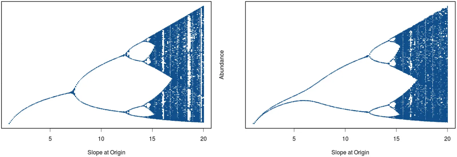
In his seminal paper on “Stock and Recruitment,” Ricker (1954) demonstrated the existence of dynamic complexity in very simple population models (see Schnute, 2006 for a review and Box 1 for details of model structure). In particular, highly convex stock-recruitment relationships can give rise to dramatic fluctuations in recruitment in these models. Ricker noted that “…[when] substantial reproduction is obtained over only a narrow range of stock densities considerably below the equilibrium level, …the stock would be subject to violent oscillations” (Ricker, 1954, p. 568²; emphasis added). Today we would recognize Ricker's apt characterization as describing a chaotic system. To see how this behavior emerges, we have plotted two cases differing in the rate of increase of recruitment at low population levels (Figure 6). In the left hand panel we see that by tracing the trajectory of change for a recruitment curve with a relatively modest rate of change at the origin, the population ultimately settles down to a fixed point equilibrium. Here, the straight line through the origin is the one-to-one replacement line and its point of intersection with the recruitment curve gives the equilibrium point. We next see that the steeper recruitment curve depicted in the right hand panel never settles down to a stable equilibrium point. At still higher values for the slope of the origin, we see the outbreak of the “violent” oscillations (chaos) reported by Ricker. The evolution of chaotic dynamics in the Ricker model follows a classical period-doubling route in which oscillations of period 2, 4, 8, …2^k emerge as the slope of the recruitment curve at the origin is increased, culminating in aperiodic dynamical behavior. Each transition to higher order oscillations represents a bifurcation point (see Box 1).

Box 1. Variations on a Theme by William Ricker.

In the following, we introduce the Ricker Model and some simple extensions to it. Ricker's equation can be written:

$\begin{array}{l}{N}_{t+1}=\alpha N_t{e}^{-\beta N_t}\end{array}$

where N_t is the population size at time t, α is the slope of the production function at the origin, and β is a coefficient of compensation. Ricker (1954) developed most of his arguments graphically. Only at the close of the paper did he present a version of his eponymous equation. As α increases, a sequence of period doubling behaviors unfolds at successive bifurcation points (see left-hand panel in Figure below).

We can readily extend the model to the multispecies case. For example, a two species model of competition can be written:

$\begin{array}{lll}{N}_{1,t+1}& =& {\alpha }_1{N}_{1,t}{e}^{-{\beta }_1{N}_{1,t}-{\delta }_{12}{N}_{2,t}}\\ N_{2,t+1}& =& {\alpha }_2{N}_{2,t}{e}^{-{\beta }_2{N}_{2,t}-{\delta }_{21}{N}_{1,t}}\end{array}$

where the subscripts 1 and 2 designate species, δ₁₂ is the effect of species 2 on species 1, δ₂₁ is the reciprocal interaction, and all other terms are defined as before Here we find that by adding consideration of species interactions to the deterministic model, oscillatory behavior with a period of two occurs at lower level of α at the origin for species 1 (right hand panel in the Figure below). In this model, we also find the emergence of “mirage” correlations to be explored in the section on State-Dependence in the text (see Figure 9).

It is not uncommon to add physical environmental terms to the model in the form:

$\begin{array}{l}{N}_{t+1}=\alpha N_t{e}^{-\beta N+\gamma E_t}\end{array}$

where E is the environmental variable (the approach can be readily extended to multiple variables). We now have a 3 dimensional surface representing the effects of spawning biomass and the environment on recruitment. We can further modify the model above to represent state-dependence in the effect of the environment:

$\begin{array}{l}{N}_{t+1}=\alpha N_t{e}^{-\beta N+\gamma N_t{E}_t}\end{array}$

where we now have an additional term representing an interaction between spawning biomass and an environmental variable. The key point is that the environmental term now enters the model in a non-additive way.

FIGURE 6

Figure 6. Cobweb diagram depicting the approach to equilibrium for a globally stable population (left panel) and the complex dynamics exhibited by a highly convex recruitment curve (right panel). The diagonal line is the one-to-one replacement line. The corresponding time series for each upper panel is show in the lower section of the figure (every point of contact between the recruitment curve and the blue cobweb iteration lines provides a point in the time series trajectory shown in the lower panels).

Beverton and Holt (1957) subsequently expanded on these concepts in their classic monograph On the Dynamics of Exploited Fish Populations (see below). In a series of highly influential articles, May (1974, 1976, 1986, 1987) brought the occurrence of seemingly random behavior in very simple (one-dimensional) deterministic models to a wider scientific audience and extended the analytical framework for understanding these systems (see also May and Oster, 1976). The intellectual excitement with the recognition of this fascinating dynamical behavior launched an extensive hunt for deterministic chaos in ecological systems.

Models in Continuous Time

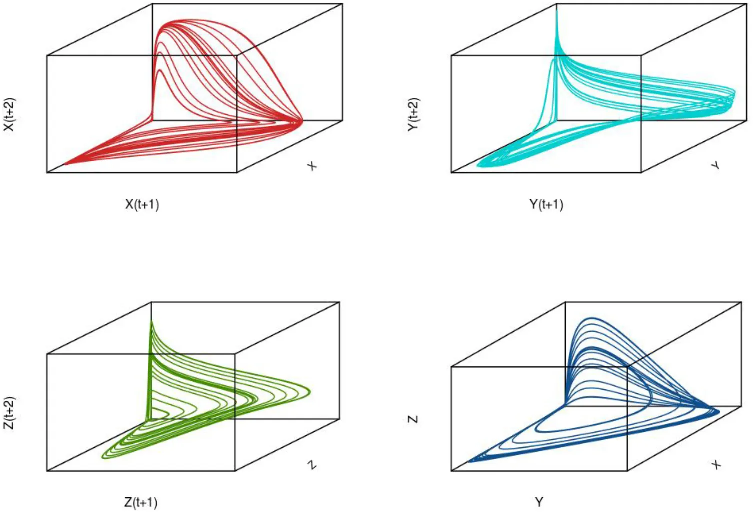
To illustrate the development of chaotic dynamics in continuous time models and to introduce the concept of a phase space representation of a system, we employ a three species system of the Lotka-Volterra type with biological interactions (competition and/or predation) among each of the species. Tanabe and Namba (2005) provide such an analysis for a simple food web comprising a basal resource species, an intermediate consumer species, and a top level omnivore that feeds on the other two species (see Box 2; for an earlier exposition see Gilpin, 1979). For certain parameter values, highly irregular irruptive population patterns can arise (see Figure 7 for population trajectories of each of the three species). If we plot the trajectories of the species in three dimensional space, we find that the highly irregular time series we observe resolve themselves into a well-defined geometrical object known as a “strange attractor” (see Figure 7 lower right panel); for context, the attractor for a globally stable equilibrium in phase space is simply a point. A key question is whether these objects are merely mathematical curiosities or whether they can be used to understand real-world dynamics³. Later we will see how we can attempt to reconstruct an attractor from time series information and test for nonlinearity.

Box 2. Models in Continuous Time.

In the absence of time delays (including seasonal forcing and time delays), the minimum number of dimensions for which complex dynamics in continuous time models can emerge is 3. Consider a three species system comprising two predators that compete for a common prey [species 1 (designated X) and species 3 (designated Z) also preys on species 3 (designated Y), (Gilpin, 1979; Tanabe and Namba, 2005)]:

$\begin{array}{l}\frac{dX}{dt}=\left[{\alpha }_1-c_{11}X-c_{12}Y-c_{13}Z\right]X,\\ \frac{dY}{dt}=\left[{\alpha }_2+c_{21}X-c_{22}Y-c_{23}Z\right]Y\\ \frac{dZ}{dt}=\left[{\alpha }_3+c_{31}X+c_{32}Y-c_{33}Z\right]Z\end{array}$

where the α_i are density-independent population coefficients and the c_ij are coefficient representing the effect of species j on species i (the c_ii are density-dependent terms). This type of community interaction is called intraguild predation. Dynamic complexity in this model is illustrated in Figure 7.

FIGURE 7

Figure 7. Time series for a three species (X,Y, Z) intraguild predation system in continuous time (see Box 3). The lower right hand panel shows the state-space representation of this system demonstrating the existence of a strange attractor.

Stochastic Resonance

Simple deterministic models cannot capture the full complexity in real systems in which exogenous forcing is important. For convenience, we will label the role of exogenous variables as stochasticity. When coupled with an underlying nonlinear dynamical system, environmental noise can be amplified⁴. In the following, we will adopt a very general definition of stochastic resonance as a situation in which the dynamical behavior of a system fundamentally changes when noise is added to an underlying deterministic process. In particular, we are interested in situations in which an underlying nonlinear process acts as a noise amplifier. This is significant in several ways. Most importantly, we find that when stochasticity is added to a nonlinear model, complex dynamics can emerge more readily than in the corresponding simple deterministic model. In many cases, it is found that in the purely deterministic case, the parameter space that gives rise to chaotic behavior is not necessarily biologically or ecologically reasonable. This has been used to argue against the likelihood of observing chaotic dynamics in real systems (e.g., Shelton and Mangel, 2011). However, adding noise can serve to radically alter the range of parameter space where we might observe complex dynamics (see Coulson et al., 2004; Sugihara et al., 2011. Interestingly, Ricker (1954) demonstrated this very point in simulations in which he added noise to highly nonlinear models (see his Figure 11, p. 575), a clear illustration of stochastic resonance. Beverton and Holt (1957; p. 57) further noted:

“..most investigations on the causes of fluctuations in natural populations have been concerned only with tracing their correlation with fluctuations in environmental factors; but …a single change in environmental conditions, either transitory or sustained, may be sufficient to set up permanent self-induced oscillations in population abundance which would bear no obvious relation to subsequent environmental changes” (emphasis added).

Steele and Henderson (1984) demonstrated that a nonlinear population process driven by periodic stochastic forcing can give rise to regime-like behavior that is consistent with observed decadal-scale patterns of variability in fish populations. Dakos et al. (2014) invoke periodic forcing combined with stochastic resonance as an underlying mechanism resulting in transitions in which critical slowing down may not be observed.

The dynamics of Dungeness crab (Cancer magister) populations on the west coast of North America exhibit the hallmarks of stochastic resonance. Dungeness crab landings in Northern California exhibit pronounced oscillatory dynamics (Figure 8). An extensive examination of endogenous dynamics and exogenous environmental forcing factors has been made in an attempt to determine the origin of these apparent cycles (Botsford and Hobbs, 1995). Simple models without demographic structure (Berryman, 1991) and more complex age-structured models (Higgins et al., 1997) show that in the absence of exogenous forcing, a stable equilibrium point is expected. However, the addition of even modest stochastic forcing in the models results in the emergence of the more complex behavior observed in the landings data. The apparent periodic behavior observed does not fall within the chaotic range (Higgins et al., 1997). Fogarty (1989) showed that the Northern California Dungeness crab catch series could be described by a (linear) autoregressive-integrated moving average model with a period of 9 years.

FIGURE 8

Figure 8. Time series of Dungeness crab (Cancer magister) landings (a proxy for abundance) in Northern California. The inset shows a time-delayed embedding of the time series reflecting periodicity in the data. This system is not chaotic.

Autocorrelated Noise

To this point, we have implicitly focused on the role of stochastic forcing by uncorrelated random processes (“white noise”). However, autocorrelated random variability in an exogenous driving variable introduces certain challenges in interpreting dynamical system behavior. In particular, it can obscure diagnostic differences in the rate of decay of forecast skill between chaotic systems and ones dominated by autocorrelated forcing. Steele (1985) noted that processes characterized by a reddened spectrum are more prevalent in marine systems than terrestrial ones⁵. Depending on the level of autocorrelation, the trajectories of these drivers may appear to exhibit regime shift-type behavior. When there is a difference in the characteristic time scale of a physical process and that of a population affected by the driver, regime-like behavior may be induced (Hsieh and Ohman, 2006). When the time scales are closer in synchrony, the population will respond in a more linear fashion to the driver. Greater divergence in synchrony can give rise to regime-like behavior. Di Lorenzo and Ohman (2013) expanded on this theme to demonstrate that a difference in the characteristic time scales of atmospheric and oceanic process may result in a reddened spectrum in the oceanographic process even when driven by a white noise atmospheric process. In turn, a difference in time scales between an autocorrelated oceanographic process and the dynamics of a pelagic population can result in an accentuated reddened spectrum for the population. Interestingly, Hsieh et al. (2005) found that environmental drivers operating at different spatial and temporal scales in the Northeast Pacific could be adequately described by linear autoregressive models and did not exhibit the hallmarks of nonlinear dynamical behavior while biological populations did exhibit the distinctive signature of complex dynamics.

Analytical Tools for Nonlinear Dynamical Systems

Evidence for nonlinear dynamics in marine systems using empirical analysis of time series data has been examined in phyto- and zooplankton communities (Sugihara and May, 1990; Ascioti et al., 1993; Belgrano et al., 2004; Hsieh et al., 2005, 2006; Benincà et al., 2008; Liu et al., 2012) and fish communities (Powers, 1991; Dixon et al., 1999; Royer and Fromentin, 2006; Anderson et al., 2008; Glaser et al., 2011, 2014; Liu et al., 2012, 2014; Sugihara et al., 2012; Deyle et al., 2013; Perretti et al., 2015; Ye et al., 2015). Most of these analyses have employed methods of state-space reconstruction.

The dimensionality of marine ecosystems is potentially very high and there are limits to the number of physical, chemical, and biological/ecological variables we can routinely monitor. Of the biological and ecological variables we can and do monitor, we can infer that they essentially encode information on other factors (e.g., other species, environmental variables, etc.) that affect their dynamics, but may be unobserved or not otherwise routinely measured. Takens (1981) showed that for nonlinear systems it is, in principle, possible to decode some of this information by translating the observed series to a system of higher order by constructing a vector of lagged observations of the original series (see Box 4). In effect, the broader dimensions of the system can potentially be captured by a more limited set of observations on one or more variables if the system is driven by nonlinear deterministic processes. To do this, we construct a time-delayed coordinate system using the lagged variables. This takes the form of a vector: X_t = (X_t,X_t−d, …X_{t−(p−1)d)}) where d is a time lag and p is the number of lags included to describe the system (referred to as the embedding dimension). Often the lag period is taken to be d = 1 but with autocorrelated series, it is desirable to have d > 1. For a system of dimensionality D, Taken's theorem states that the properties of lagged coordinate systems is equivalent to that of the original state space when the embedding dimension p is >2D + 1. In practice, it is often substantially less when determinism is high.

Takens' (1981) key insight was that the basic properties of the state space for the overall system can be reconstructed by examining the time-delayed structure of just one of the variables. The resulting geometric shape in state space is directly related to the true underlying attractor, giving a “shadow” attractor which, as noted above, retains the dynamical properties of the original provided a sufficient number of lags have been incorporated. When this condition is met, the Lyapunov exponent, a diagnostic measure of chaos (see Box 3) of the shadow attractor is the same as that of the original. Although, state space reconstruction cannot of course identify the unobserved variables of importance, we can make important inferences about the effective dimensionality and degree of nonlinearity in the system. All methods of nonlinear time series analysis used to assess dynamic complexity employ time-delay coordinate systems as the foundation for determining the dimensionality and nonlinearity of the system (for a readable account, see Kaplan and Glass, 1995).

Box 3. Quantifying Chaos using Lyapunov Exponents.

Chaotic systems are characterized by sensitive dependence on initial conditions. Give two initial starting points, the distance between these two trajectories diverge exponentially with successive time steps in a chaotic system. For a globally stable system in contrast, the distance between two initial conditions converges with successive iterations. Using this simple concept as a starting point, we can measure the average rate of divergence or convergence over an attractor to characterize the dynamics of the system.

We first define the separation distance of two starting values x_o and $x_{o\prime }$ as

$\begin{array}{l}{\delta }_o=|x_o-x_{o^{\prime }}|\end{array}$

For simplicity, we have assumed that the starting values lie on the attractor and there are no transients at the start of the series. We are interested in the magnitude of the separation distances between the trajectories, but not their direction (sign) and so we take absolute values. The difference after N iterations is:

$\begin{array}{l}{\delta }_N=|x_N-x_{N^{\prime }}|\end{array}$

and the relationship between δ_N and δ_o is given by:

$\begin{array}{l}{\delta }_N={\delta }_o{e}^{\lambda N}\end{array}$

where λ gives the slope of this relationship. This slope gives a local rate of divergence or convergence for these starting conditons. We are interested in the average slope over all starting conditions (and sections of the attractor). The largest value of this quantity is given by:

$\begin{array}{l}\lambda *={\displaystyle \underset{N\to \infty }{lim}}\frac{1}{N}{\displaystyle \sum _{i=0}^{n-1}}{log}_e\frac{{\delta }_N}{{\delta }_o}\end{array}$

This is called the Lyapunov exponent. A positive Lyapunov exponent is diagnostic of chaos. A negative value indicates a stable system.

The time-evolution of nearby points in state space emerges as a critical consideration in understanding and classifying complex dynamical behavior. Formals tests for chaos based on the Lyapunov exponent depend on measures of the rate divergence of points over time derived from points starting in very close proximity in state space (refer to Box 3). Because regions of state space of a chaotic system are expected to be revisited in arbitrarily close proximity, methods based on estimating the recurrence of observations in state space have also been used to detect nonlinear dynamics (e.g., Kaplan and Glass, 1995, pp. 315–318; Kantz and Schreiber, 2003, pp. 44–45). Royer and Fromentin (2006) provide an application of recurrence mapping to extensive catch histories of Atlantic bluefin tuna in the Mediterranean.

Turchin and Taylor (1992) proposed the use of a parametric model based on polynomial regression (see Box 4) to construct response surfaces for the time delayed coordinate system. It is then possible to test formally for evidence of nonlinear dynamics (Ellner and Turchin, 1995) by estimating the parameters of the polynomial; making forward projections from the model; and empirically determining the Lyapunov exponent by measuring the rate of divergence of near-by points in phase space. The response surface methodology is based on familiar model forms and is easy to apply with standard statistical software. For short time series it has been suggested that it may hold advantages over other methods that require more data for fitting (Ellner and Turchin, 1995).

Box 4. Time Series Methods for State Space Reconstruction.

Approaches that have been used to estimate parameters describing the internal dynamics of the time-delayed coordinate system including a parametric modeling approach based on response surface methodology (Turchin and Taylor, 1992) and a number of non-parametric representations including piece-wise polynomial approximations (splines; McCaffrey et al., 1992); neural networks (Nychka et al., 1992); and a combined sequential strategy using nearest neighbor forecasting methodology to determine the embedding dimension coupled with a kernel regression method to determine the degree of nonlinearity (Sugihara and May, 1990). For illustration, in the following we will focus on just two of these approaches, the response surface methodogy of Turchin and Taylor, 1992) and the kernel regression method of Sugihara (1994). The reader is referred to the excellent reviews by Ellner and Turchin (1995) and Hastings et al. (1993) for further details on these and additional methods in state space reconstruction. In the illustration below, we show the shadow attractors for each of the three variables in the intraguild predation model described earlier (see Figure 6) along with true underlying attractor (lower right panel).

The Turchin and Taylor (1992) approach employs a generalized polynomial of the form:

$\begin{array}{l}{log}_e\left(\frac{N_{t+1}}{N_t}\right)=g\left(N_t^{{\Theta }_1}{N}_{t-1}^{{\Theta }_2},N_{t-2}^{{\Theta }_3},\dots N_{t+1-d}^{{\Theta }_d}\right)\end{array}$

where the Θ_i are coefficients for the Box-Cox transformation which includes many standard transformations (e.g., logarithmic, square root etc.) as special cases. The expression on the left hand side of the equation is the natural logarithm of the replacement rate. The model can be fit by nonlinear regression when the Θ_Iare free parameters. Alternatively, a range of fixed values for the Θ_i can be applied for all possible combinations and the best fitting model selected. Once the form of the model has been determined, it can be used to simulation population trajectories for different starting values. The rate of divergence of the trajectories for different initial conditions can then be determined to provide an empirical estimate of the Lyapunov function.

In contrast, Sugihara and May (1990) employ nonparametric estimators and rely on measures of forecast skill for model selection. A form of kernel regression to estimate the degree of nonlinearity in a system with embedding dimension d is used. Specifically, a forecast of X(t*+p) from the state space vector x(t*) reconstructed from the lagged coordinate system is made using a linear model C:

$\begin{array}{l}\widehat{X}\left(t^{*}+p\right)=C_o+{\displaystyle \sum _{j=0}^{E-1}}{c}_j{x}_j\left(t^{*}\right)\end{array}$

where the scaling factor c is estimated using a form of Principal Components Analysis for the system of equations:

$\begin{array}{l}\mathbf{B}=\mathbf{A}\mathbf{C}\end{array}$

where B is a vector of dimension n of weighted future values X_t for each observed time t:

$\begin{array}{l}{B}_i=w\left(\left|\right|x_t-x^{*}\left|\right|\right)X_i\left(t+p\right)\end{array}$

and A is an n × d dimensional matrix with elements:

$\begin{array}{l}{A}_{ij}=w\left(\left|\right|x_t-x^{*}\left|\right|\right)X_i\left(t\right)\end{array}$

Because A is a non-square matrix, the solution (which requires inverting A) employs singular value decomposition.

The weighting function w is defined as

$\begin{array}{l}w\left(d\right)=e^{{}^{-\theta d}{╱}_{\overline{d}}}\end{array}$

where the parameter Θ determines the degree of nonlinearity in the system (system is linear for Θ = 0 and nonlinear for Θ > 0). The expression is normalized by distance between x(t*) and the observed points x(t):

$\begin{array}{l}\overline{d}=\frac{1}{n}{\displaystyle \sum _{j=1}^n}\left|\right|x\left(t\right)-x\left(t^{*}\right)\left|\right|\end{array}$

In principle, it is possible to search over all combinations of the embedding dimension d and values of the shape parameter Q to determine the choice that provides the greatest skill in out-of-sample forecasts. However, the search time for such an exercise can be extensive. Sugihara and May (1990) recommend an alternative approach in which the dimensionality of the system is first determined using a nearest neighbor forecasting algorithm.

Examples of nonparametric models used to fit lagged variables include applications of neural networks (Nychka et al., 1992); thin-plate splines (McCaffrey et al., 1992); and the combined application of nearest neighbor simplex algorithms (to estimate dimensionality) and a variant on kernel regression to estimate nonlinearity (Sugihara and May, 1990, see Box 4). In the following, we will focus on the latter because it is the approach most frequently applied to marine systems to date. The nonparametric (“equation-free”) approach has the virtue of attacking the problem of model uncertainty in an innovative way (see DeAngelis and Yurek, 2015). We often do not fully understand the processes operating at the population, community, and ecosystem levels and the combination of state-space construction and flexible non-parametric approaches offers a potential (and powerful) alternative approach to structural models.

While the methods of Turchin and Taylor (1992) and Ellner and Turchin (1995) are expressly used to test for chaotic dynamics, the Sugihara and May (1990) approach focuses on distinguishing between linear and nonlinear dynamics and Lyapunov exponents are not directly calculated. Here, the forecast skill of the nonlinear model is tested against a null linear vector autoregressive model. Assessing out-of-sample forecast skill in which some data (typically at the end of the series) are held in reserve for testing is the preferred approach. However, for shorter time series, it is often necessary to use cross-validation studies instead in which one or more observations within the series are randomly removed, the model fit to the remaining points, and predictions for the removed points compared with the observed.

State-Dependence

Here, state-dependence will be taken to refer to situations in which the effect of one variable on another is conditioned on the state of an explanatory variable. In an early suggestive example, Skud (1982) identified cases in which the sign of a correlation between landings (taken as an index of abundance) and temperature of Atlantic herring (Clupea harengus) and Atlantic mackerel (Scomber scombrus) off New England changed during different stanzas of time depending on whether herring or mackerel were more abundant. In this case, the abundance proxy is the state variable of interest. Skud (1982) reported similar results for California sardine (Sardinops sagax) and anchovy (Engraulis mordax). Using multivariate nonlinear time series models, Sugihara et al. (2012) and Deyle et al. (2013) confirmed the existence of state dependence in the relationship between California sardine abundance and temperature.

Brander (2005) combined information for 6 Atlantic cod (Gadus morhua) stocks in the Northeast Atlantic and partitioned the spawning stock and recruitment values of each into high, medium, and low categories. A similar categorization scheme was applied to values of the North Atlantic Oscillation (NAO). Brander found that under low (negative) NAO conditions, the probability of low recruitment at low spawning stock sizes was significantly higher than when positive NAO conditions prevailed.

State-dependence can lead to “mirage” correlations (Sugihara et al., 2012) in which functionally related series can appear to change synchronously or asynchronously over different stanzas of time depending on the state of different elements in the system (Figure 9). In this situation, Bishop Berkeley's famous aphorism can be reversed: lack of correlation does not (necessarily) imply a lack of causation (Sugihara et al., 2012).

FIGURE 9

Figure 9. Simulated time series for a two species competitive system showing strongly correlated (I), uncorrelated (II), weakly correlated (III), and anti-correlated (IV) stanzas for the multispecies Ricker model described in Box 1.

Causality

Our discussion of state-space reconstruction has centered on analysis of a single time series. Extending our frame of reference from the univariate case to a multidimensional view of system dynamics offers opportunities not only for improved forecast skill, but for inferring causal connections among observed system elements. Deyle and Sugihara (2011) developed a multivariate extension of Takens' embedding theorem that sets the stage for this approach.

Granger (1969) proposed that for stochastic systems, causality could be inferred for the case where including one or more “explanatory” variables in an analysis increases the prediction skill for a “response” variable. For deterministic multivariate systems however, another approach is required. In effect, issues related to state-dependence in a nonlinear dynamical system make it impossible to truly separate the component parts. Sugihara et al. (2012) tackle this problem by reconstructing the attractors for each series using lagged coordinate systems. If information on one attractor at a given time point can be used to effectively predict the state of the other attractors, a direct causal connection is inferred. The concept of Granger Causality can therefore be extended to systems with a strong nonlinear deterministic component. This approach has been used to examine evidence for causal connections between environmental drivers and abundance of Pacific sardine (Deyle et al., 2013) and sockeye salmon (Ye et al., 2015). This focus on predictability as measure of model performance resonates with earlier calls for the development of a predictive ecology (e.g., Peters, 1991).

Fisheries as Complex Systems

Fisheries lie at the intersection of an interwoven set of ecological, social, economic, and governance considerations. Although, fisheries are now widely recognized as a major social-ecological system type providing a critically important ecosystem service, far less is known concerning the full implications of the interplay between ecosystem and social dynamics in this context. Allen and McGlade (1986, 1987) provided one of the first formal explorations of fisheries as complex systems. Worldwide initiatives are now underway to transform management of marine systems using a more holistic approach incorporating fundamental ecosystem principles treating humans as in integral part of the ecosystem. A key element in this transformation is the recognition that a much broader palette of dynamical responses to human intervention and impacts must be entertained (Fogarty, 2014). In the following, we examine ways in which harvesting can change the dynamical behavior of ecosystems.

Glaser et al. (2014) examined this fundamental issue in a comparative analysis of over 200 taxa in two marine ecosystems, the California Current System and Georges Bank. Abundance indices based on both fishery-dependent (e.g., catch-per-unit effort) and fishery independent data (scientific surveys) were used in conjunction with information on catch data to ask whether differences in estimated dimensionality and degree of nonlinearity could be detected in these very different data types. Differences in system dimensionality and nonlinearity were found and associated with human intervention through fishing, implying that the coupling between human and natural systems generated dynamics distinct from those detected in the natural subsystem alone. Such patterns have been previously examined in other coupled social-ecological system types (Liu et al., 2007; Horan et al., 2011).

Glaser et al. (2014) reported that catch data exhibited the highest level of dimensionality, followed by abundance of exploited species, and abundance of non-exploited species in that order. The catch series were significantly less predictable than the corresponding abundance measures for individual species. The observed catch data presumably reflects not only the underlying dynamics of the resource base, but a sequence of interactions including fishermen behavior and choice, costs, market conditions, and regulations on fishing effort resulting in a form of layered complexity in the fishery system as a whole.

Fishing and Dynamical Response

We have seen in the context of catastrophe theory that fishing can induce sudden changes in state of the resource. Both fold and cusp catastrophes have been invoked to explain sudden population collapse in ecosystems. More generally, in nonlinear systems, fishing and other anthropogenic stressors can strongly alter the dynamic landscape, either inducing or dampening the expression of dynamic complexity. In the following, we will provide different illustrations of how these differences can emerge.

Myers et al. (1998) proposed that a form of stochastic resonance could underlie the phenomenon of cyclic dominance in Sockeye salmon (Onchorhyncus nerka). Sockeye salmon in British Columbia have a 4 year life cycle (although a small fraction return to their native rivers to spawn and die after 5 years). Cyclic dominance refers to the disparity in population size of different “lines” of sockeye giving rise to 4-year cycles in a number of populations. Ricker (1997) reviewed potential underlying ecological and fishery-related mechanisms giving rise to this fascinating periodic pattern (Figure 10; upper panel). Myers et al. (1998) showed that the interplay of harvesting and stochastic forcing can recreate basic patterns of this type for certain ranges of the parameter space and exploitation levels in a Ricker model (see Box 5). In the absence of random perturbation, stable equilibria are obtained for all four lines. Myers et al. (1998) found that when applying estimated parameter values derived from a meta-analysis of sockeye salmon stocks with no external forcing and catch levels within the normal range of the fishery, a stable equilibrium was obtained. However, when environmental variability was added to the model, a 4-year cycle similar to observed sockeye patterns was obtained (Figure 10; lower panel). Interestingly, this result holds only for certain ranges of the catch and levels of random variability and these coincide with past observation. This form of stochastic resonance involves a specific interaction between human intervention through harvesting and environmental variability.

FIGURE 10

Figure 10. Population index values for Sockeye Salmon (Onchyrhyncus nerka) from the Shaswap River, British Columbia (upper panel; source: Ye et al., 2015) and simulated time series using the method of Myers et al. (1998; see Box 5) demonstrating stochastic resonance (lower; the horizontal line shows the equilibrium series generated with no stochastic forcing).

Box 5. Effects of Exploitation on Dynamical Behavior.

In the following, we explore four examples of incorporating fishing mortality in models at the population and community levels.

Myers et al. (1998) proposed a mechanism underlying the famous 4 year cycles in Sockeye salmon (Onchorhyncus nerka) based on a modification of the Ricker model to reflect harvest pressure and stochastic forcing:

$\begin{array}{l}{N}_{t+4}=\alpha \left(1-H_t\right)N_t{e}^{-\beta N_t+{\epsilon }_t}\end{array}$

where H_t is the fractional harvest rate in year t, ε_t is a white noise random perturbation with mean 0 and constant standard deviation σ_ε and all other terms are defined as before. Myers et al. reported that for observed levels of H~0.75–0.8 and σ_ε ~0.8 derived from observed sockeye populations, pronounced 4 year cycles can be produced. This topic is explored further in the section on Stochastic Resonance in the text (see Figure 10).

To explore the implications of age or size-specific harvesting, we can incorporate a form of simplified demographic structure comprising juveniles (designated by the subscript J) and adults (A):

$\begin{array}{l}{N}_{t+1}=s_{A,t}{N}_{A,t}+s_{J,t,}\alpha N_{A,t+1-r}{e}^{-\beta N_{A,t+1-r}}\end{array}$

where s_A = exp[-(F_{A, t+}M_{a, t})] is the fractional survival rate of adults in year t, F_{A, t} is the instantaneous rate of fishing mortality imposed on adults in year t and M_{A, t} is the instantaneous rate of natural mortality of adults due to predation, disease, and other factors. For juveniles, we have s_J = exp(-rF_J) where r is the duration of the juvenile phase; the term α already incorporates natural mortality during the juvenile phase in this formulation. In the following, we will simplify the model to fit the case where the adults produce juveniles which become adults after 1 year (r = 1). The first term on the right hand side of the equation therefore gives the number of adults surviving from the previous time year and the second term is the number of juveniles entering the adult stage in year t+1. In Figure 11 we explore two cases: (a) only adults are exploited and (b) both juveniles and adults are harvested. In the upper panel of Figure 11 we vary the adult survival rate by changing the fishing mortality rate on adults while prohibiting fishing on juveniles. In the lower panel of Figure 11 we impose a constant level of fishing on juveniles while again varying adult survival by changing the fishing mortality rate on adults.

We next turn to a simple predator-prey model in discrete time (Basson and Fogarty, 1997). The model for the prey (species 1) and the predator (species 2) can be written:

$\begin{array}{l}{N}_{1,t+1}={\alpha }_1{N}_1{e}^{-{\beta }_1{N}_{1,t}-{\delta }_{12}{N}_{2,t}-F_1}\end{array}$

$\begin{array}{l}{N}_{2,t+1}={\alpha }_2{N}_{2,t}{e}^{-{\beta }_2{N}_{2,t}+{\delta }_{21}{N}_{1,t}-F_2}\end{array}$

where the sign of the δ_ij indicates the nature of the interactions (the predator has a negative effect on the prey and the prey has a positive effect on the predator through the conversion of prey numbers into predator abundance. Here our interest centers on how the fishing mortality rates(F) exerted on each species affects the expression of complex dynamics of this simple community and the F.

As a final example, we examine the effects of fishing on the three species system described by Hastings and Powell (1991). In this model, a basal resource species (species 1 designated X) is preyed on by an intermediate predator (species 2 designated Y) and this predator in turn is preyed on by a top-level predator (species 3 designated Z). In both instances, the predators exhibit a saturating functional feeding response:

$\begin{array}{l}\frac{dX}{dt}=\left[{\alpha }_1-c_{11}X-\frac{A_{1}X}{B_1+X}Y\right]X_{,}\\ \frac{dY}{dt}=\left[C_2\frac{A_{1}X}{B_1+X}-\frac{A_{2}Y}{B_2+Y}Z-D_2-F_2\right]Y\\ \frac{dZ}{dt}=\left[C_3\frac{A_{1}Y}{B_1+Y}-D_3-F_3\right]Z\end{array}$

where a₁ is the intrinsic rate of increase of X and c₁₁ is an intraspecific interaction term; the A_i and B_i are coefficients of the functional feeding response of species i; the C_i are prey conversion efficiencies for species i; the D_i are mortality terms due to causes other than predation and fishing; and the F_i are fishing mortality rates imposed on species i (see Figure 13). For an alternative parameterization of this model see McCann and Yodzis (1994).

Size- or age-selective harvesting practices can also affect the expression of complex dynamics in exploited marine species. For example, in populations with multiple age classes, selectively harvesting older age classes can be destabilizing when nonlinear dynamics originates in processes affecting the younger life stages. In this case, the stabilizing effect of maintaining a broad portfolio of age classes is degraded as the survival rate of older age classes declines due to harvesting (Figure 11 upper panel). The underlying complex dynamics generated during the early part of the life cycle can be effectively masked under low exploitation rates. Anderson et al. (2008) further note that this decreased stability can also reflect induced changes in the intrinsic rate of increase in exploited populations subject to juvenescence. Thus, the observation by Glaser et al. (2011) of higher levels of nonlinearity in exploited populations relative to unexploited ones may reflect, in part, the effect of size-specific harvesting strategies in which larger individuals are targeted. In contrast, when harvesting affects both older individuals and some fraction of the younger age classes, the expression of complex dynamics can be substantially altered relative to the case where only adults are harvested (Figure 11 lower panel).

FIGURE 11

Figure 11. Bifurcation diagrams for a simple age-structured model in which (A) harvesting is exerted only on the older age classes and (B) when 40% of the juveniles are also exploited.

If we increase the dimensionality of the system to include more than one species, the range of possibilities for dynamical behavior further increases. For example, Basson and Fogarty (1997) show that in a two-species production model with no age or size structure, an examination of the state space framed by the fishing pressure on each species reveals islands of complexity where stable, cyclic, and chaotic behaviors exist in different (but intermixed) regions of the exploitation landscape (Figure 12). Human choice with respect to the relative fishing intensities imposed on the predator and prey strongly affects the expression of complex dynamics. In this case, understanding the underlying processes is essential in understanding whether avoiding actions that will induce complex dynamics is at all possible.

FIGURE 12

Figure 12. Dynamical landscape for an exploited two-species predator-prey system using a simple Lotka-Volterra type production model. Regions of the exploitation phase space for complex (blue), cyclic (red), and stable (green) dynamics are shown. The interplay between harvesting, species interactions, and the internal dynamics of the two species generates islands of complexity in the landscape (adapted from Figure 3 of Basson and Fogarty, 1997).

Hastings and Powell (1991) traced the development of complex dynamics in a three-species system comprising a simple linear food chain with a basal resource species and two predators. In this case, the predators have a saturating functional feeding response, distinguishing it from the intraguild predation model we examined in Box 2 (see Figure 7). We can explore the implications of adding fishing to this system (see Box 5). In the absence of exploitation, the time trajectories of the three species do not attain a simple stable equilibrium for parts of the parameter space and a strange attractor emerges (Hastings and Powell, 1991, Figure 13) left column. However, introducing a simple form of harvesting in which yield is extracted in proportion to the population size of the prey dampens the expression of complex dynamics for this same range of parameter space. Even for a relatively low level of fishing mortality (F = 0.2), the system switches from chaotic dynamics to a limit cycle (Figure 13 middle column). For a higher level of exploitation (F = 0.4), the system settles down to a stable equilibrium point (Figure 13 right column).

FIGURE 13

Figure 13. Dynamics of a predator-prey system comprising three species: X (upper row), Y (middle row), and Z (lower row). The fourth row shows the three-dimensional attractors for the system. The first column shows results for no fishing (Hastings and Powell 1991); the middle column shows results of adding low to moderate fishing (F = 0.2); and the third column shows results for higher fishing mortality (F = 0.4).

The main message that emerges from these examples is that the exact nature of human intervention, coupled with the form of the nonlinear processes governing the system dynamics, can strongly alter the expression of dynamic complexity. In a single species context, non-selective harvesting can hold very different implications than size or age-selective patterns of exploitation. Adding consideration of environmental variability and species interactions can further alter the dynamical landscape. The application of empirical methods of state-space reconstruction in effect allows the data to speak. Given the uncertainty in our understanding of system dynamics and underlying governing processes, this approach offers a potentially powerful complement to more traditional methods based on structural equation modeling.

Other Forms of Human Intervention

We note that in the quest for enhanced yields from marine ecosystems, humans have altered these systems in many ways. These alterations encompass not only removal of biomass from natural populations through catches but supplementing natural populations through large-scale hatchery operations. Young fish (or shellfish) are grown through the critical early life stages during which mortality rates are typically high, and then released to augment the natural population for subsequent harvest. The number of Pacific salmon released from hatchery systems is in the billions and considerable controversy over the efficacy and potential environmental impacts of artificial enhancement of this type exists (Naish et al., 2008). Fagen and Smoker (1989) raised the interesting question of whether large-scale introduction of hatchery-reared salmon could alter the expression of complex dynamics in the population. In particular, because the hatchery operation is intended to deliberately increase the juvenile survival rate during a vulnerable period of the life history, it is important to know whether this change could be manifest in the emergence of complex dynamics. Fagen and Smoker (1989) show that an effective increase in the intrinsic rate of increase of the population given a sufficiently large hatchery production can in fact lead to complex dynamics. Although, no empirical analyses have been undertaken to explore evidence for the effects of hatchery operations on the expression of dynamic complexity, McCarl and Rettig (1983) had earlier noted an increase in variability in Pacific salmon returns with increasing hatchery releases.

Conclusions

As noted in the Introduction, complexity theory emerged from earlier developments in nonlinear dynamics (bifurcation theory, catastrophe theory, and chaos theory). Complexity theory goes beyond its antecedents, however, in focusing on issues such as the emergent properties of complex systems and concepts such as “order out of chaos” (e.g., Waldrop, 1992). In this construct, systems characterized by Lyapunov exponents ~0 are most likely to exhibit these properties. Some evidence from ecological systems suggests a mode in the distribution of Lyapunov exponents calculated from a broad array of natural and laboratory populations consistent with this concept (Ellner and Turchin, 1995). While chaotic systems exhibit strong dependence on initial conditions and short term memory in system dynamics, the behavior of complex systems is more typically associated with the importance of past history in shaping the future. In fisheries systems, there is substantial evidence that higher levels of ecological organization such as guilds and communities are often more stable and predictable than lower levels (populations and species), possibly reflecting emergent properties in these systems (e.g., Fogarty and Murawski, 1998; Fogarty, 2014).

Recognition of the potential for complex dynamical behavior in exploited marine ecosystems calls for a paradigm shift in fisheries management. In particular, the fundamental premise that fishery systems are governed by globally stable dynamics leads to the possibility of sudden and unanticipated shifts in resource and ecosystem status that hold profound ecological, social, and economic consequences when these assumptions are not met. Again, the difficulty lies not in the broader conceptual framework of fisheries science, in which these possibilities have been identified and explored, but rather in the narrower frame of reference typically adopted in management practices. In particular, the dominant management paradigm centered on the concept of maximum equilibrium yield sets the stage for unexpected surprises in population and/or ecosystem status. Resource managers should instead be prepared for the unexpected and act accordingly.

Author Contributions

MF conceived and wrote the paper. All authors contributed to its final form.

Conflict of Interest Statement

The authors declare that the research was conducted in the absence of any commercial or financial relationships that could be construed as a potential conflict of interest.

Acknowledgments

We extend our appreciation to Geir Huse and Fabio Lamantia for their helpful comments on the manuscript and to Michael St. John for his editorial guidance. We are grateful to George Sugihara, Ethan Deyle, Hao Ye, Hui Liu and Sarah Glaser for fruitful collaboration and discussion over the last several years.

Footnotes

1. ^Linear dynamical behavior is evident in models with nonlinear structural forms for ranges of the parameter space resulting in globally stable equilibria. Some of these models can also exhibit non-linear dynamical behavior for certain ranges of the parameter space.

2. ^Ricker (1954) noted that when the slope of the descending limb of the recruitment curve was < −1, unstable dynamics resulted.

3. ^The existence of a recognizable attractor is not in itself diagnostic of nonlinear dynamics. For example a random series comprising a periodic signal and superimposed autocorrelated noise can give a geometric object in phase space that appears similar to a strange attractor. Diagnostic tests described below must be used to confirm the occurrence of nonlinear dynamics (see Boxes 3, 4).

4. ^Hastings et al. (1993) and Ellner and Turchin (1995) argue that no broad dividing line between chaos and stochasticity should be drawn. However, noting that the pathway to chaos in systems exhibiting stochastic resonance as defined here differs from those leading to deterministic chaos, Dennis et al. (2003) recommend that the term “Noise-induced Sensitivity” be used to distinguish deterministic chaos from stochastic resonance.

5. ^Time series with reddened spectra exhibit increased variance with increasing length in association with temporal autocorrelation.

References

Allen, P. M., and McGlade, J. M. (1986). Dynamics of discovery and exploitation: the case of the Scotian Shelf groundfish fisheries. Can. J. Fish. Aquat. Sci. 43, 1187–1200. doi: 10.1139/f86-148

CrossRef Full Text | Google Scholar

Allen, P. M., and McGlade, J. M. (1987). Modelling complex human systems: a fisheries example. European J. Operat. Res. 30, 147–167. doi: 10.1016/0377-2217(87)90092-0

CrossRef Full Text | Google Scholar

Anderson, C. N. K., Hsieh, C. H., Sandin, S. A., Hewitt, R., Hollowed, A., Beddington, J., et al. (2008). Why fishing magnifies fluctuations in fish abundance. Nature 452, 835–839. doi: 10.1038/nature06851

PubMed Abstract | CrossRef Full Text | Google Scholar

Ascioti, F. A., Beltrami, E., Carrol, T. O., and Chreighton, W. (1993). Is there chaos in plankton dynamics? J. Plank. Res. 15, 603–617. doi: 10.1093/plankt/15.6.603

CrossRef Full Text | Google Scholar

Bakun, A. (2004). “Regime shifts,” in The Sea, Vol. 13, eds A. R. Robinson and K. Brink (New York, NY: J. Wiley and Son), 971–1018.

Basson, M., and Fogarty, M. J. (1997). Harvesting in discrete-time predator-prey systems. Math. Biosc. 141, 41–74. doi: 10.1016/S0025-5564(96)00173-3

PubMed Abstract | CrossRef Full Text | Google Scholar

Baumgartner, T., Soutar, A., and Ferreira-Bartrina, V. (1992). Reconstruction of the history of Pacific sardine and northern anchovy populations over the past two millennia from sediments of the Santa Barbara Basin, California. CalCOFI Rep 33, 24–40.

Lluch-Belda, D., Crawford, R. J. M., Kawasaki, T., MacCall, A. D., Parrish, R. H., Schwartlose, R. A., et al. (1989). Worldwide fluctuations of sardine and anchovy stocks: the regime problem. S. Afr. J. Mar. Sci. 8, 195–205. doi: 10.2989/02577618909504561

CrossRef Full Text | Google Scholar

Belgrano, A., Lima, M., and Stenseth, N. C. (2004). Non-linear dynamics in marine phytoplankton population systems. Mar. Ecol. Prog. Ser. 273, 281–289. doi: 10.3354/meps273281

CrossRef Full Text | Google Scholar

Benincà, E., Huisman, J., Heerkloss, R., Johnk, K. D., Branco, P., Van Nes, E. H., et al. (2008). Chaos in a long-term experiment with a plankton community. Nature 451, 822–825. doi: 10.1038/nature06512

PubMed Abstract | CrossRef Full Text | Google Scholar

Berryman, A. A. (1991). Can economic forces cause ecological chaos? The case of the northern California Dungeness crab fishery. Oikos 62, 106–109.

Google Scholar

Beverton, R. J. H., and Holt, S. J. (1957). On the Dynamics of Exploited Fish Populations. London: Chapman & Hall.

Google Scholar

Biggs, R., Carpenter, S. R., and Brock, W. A. (2009). Turning back from the brink: detecting an impending regime shift in time to avert it. Proc. Nat. Acad. Sci. U.S.A. 106, 826–831. doi: 10.1073/pnas.0811729106

PubMed Abstract | CrossRef Full Text | Google Scholar

Botsford, L. W., and Hobbs, R. C. (1995). Recent advances in the understanding of cyclic behavior of Dungeness crab (Cancer magister) populations. ICES J. Mar. Sci. 199, 157–166.

Google Scholar

Brander, K. (2005). Cod recruitment is strongly affected by climate when stock biomass is low. ICES J. Mar. Sci. 62, 339–343. doi: 10.1016/j.icesjms.2004.07.029

CrossRef Full Text | Google Scholar

Brock, W. A., and Carpenter, S. R. (2006). Variance as a leading indicator of regime shift in ecosystem services. Ecol. Soc. 11, 9. Available online at: http://www.ecologyandsociety.org/vol11/iss2/art9/

Caddy, J. F., and Gulland, J. A. (1983). Historical patterns of fish stocks. Mar. Pol. 7, 267–278. doi: 10.1016/0308-597X(83)90040-4

CrossRef Full Text | Google Scholar

Casti, J. L. (1994). Complexification: Explaining a Paradoxical World Through the Science of Surprise. New York, NY: Harper-Collins.

Google Scholar

Chavez, F. P., Ryan, J., Lluch-Cota, S., and Miguel Ñiquen, C. (2003). From anchovies to sardines and back: multidecadal change in the Pacific Ocean. Science 299, 217–222. doi: 10.1126/science.1075880

PubMed Abstract | CrossRef Full Text | Google Scholar

Collie, J. S., Richardson, K., and Steele, J. H. (2004). Regime shifts: can ecological theory illuminate the mechanisms? Prog. Oceanogr. 60, 281–302. doi: 10.1016/j.pocean.2004.02.013

CrossRef Full Text | Google Scholar

Coulson, T., Rohani, P., and Pascual, M. (2004). Skeletons, noise, and population growth: the end of an old debate? Trends Ecol. Evol. 19, 359–364. doi: 10.1016/j.tree.2004.05.008

PubMed Abstract | CrossRef Full Text | Google Scholar

Dakos, V., Carpenter, S. R., van Nes, E. H., and Scheffer, M. (2014). Resilience indicators: prospects and limitations for early warnings of regime shifts. Philos. Trans. R. Soc. B 370, 20130263. doi: 10.1098/rstb2013.0263

CrossRef Full Text | Google Scholar

DeAngelis, D. L., and Yurek, S. (2015). Equation-free modeling unravels the behavior of complex ecological systems. Proc. Natl. Acad. Sci. 112, 3856–3857. doi: 10.1073/pnas.1503154112

PubMed Abstract | CrossRef Full Text | Google Scholar

Dennis, B., Desharnais, R. A., Cushing, J. M., Henson, S. M., and Costantino, R. F. (2003). Can noise induce chaos? Oikos 102, 329–339. doi: 10.1034/j.1600-0706.2003.12387.x

CrossRef Full Text | Google Scholar

Devaney, J. (1989). An Introduction to Chaotic Dynamical Systems, 2nd Edn. Boulder, CO: Westview Press.

Deyle, E. R., and Sugihara, G. (2011). Generalized theorems for nonlinear state space reconstruction. PLoS ONE 6:e18295. doi: 10.1371/journal.pone.0018295

PubMed Abstract | CrossRef Full Text | Google Scholar

Deyle, M., Fogarty, M. J., Hsieh, C.-H., Kaufman, L., MacCall, A. D., Munch, S. B., et al. (2013). Climate effects on Pacific Sardine. Proc. Natl. Acad. Sci. U.S.A. 110, 6430–6435. doi: 10.1073/pnas.1215506110

PubMed Abstract | CrossRef Full Text | Google Scholar

Di Lorenzo, M., and Ohman, M. (2013). A double-integration hypothesis to explain ocean ecosystem response to climate forcing. Proc. Natl. Acad. Sci. U.S.A. 110, 2496–2499. doi: 10.1073/pnas.1218022110

PubMed Abstract | CrossRef Full Text | Google Scholar

Dixon, P. A., Milicich, M. J., and Sugihara, G. (1999). Episodic fluctuations in larval supply. Science 283, 1528–1530.

PubMed Abstract | Google Scholar

Ellner, S., and Turchin, P. (1995). Chaos in a noisy world: new methods and evidence from time-series analysis. Am. Nat. 145, 343–375. doi: 10.1086/285744

CrossRef Full Text | Google Scholar

Evans, G. (1981). The potential collapse of fish stocks in a developing fishery. N. Am. J. Fish. Mgt. 1, 127–133.

Google Scholar

Fagen, R., and Smoker, W. W. (1989). How large-capacity hatcheries can alter interannual variability of salmon production. Fish. Res. 8, 1–11. doi: 10.1016/0165-7836(89)90036-2

CrossRef Full Text | Google Scholar

Fogarty, M. J. (1989). “Forecasting yield and abundance of exploited invertebrates,” in Marine Invertebrate Fisheries: Their Assessment and Management, ed J. F. Caddy (New York, NY: John Wiley and Sons), 701–724.

Fogarty, M. J. (2014). The art of ecosystem-based fishery management. Can. J. Fish. Aquat. Sci. 71, 479–490. doi: 10.1139/cjfas-2013-0203

CrossRef Full Text | Google Scholar

Fogarty, M. J., and Murawski, S. A. (1998). Large-scale disturbance and the structure of marine systems: fishery impacts on Georges Bank. Ecol. Appl. 8, 6–22. doi: 10.2307/2641359

CrossRef Full Text | Google Scholar

Fogarty, M. J., Rosenberg, A. R., and Sissenwine, M. P. (1992). Fisheries risk assessment - sources of uncertainty; a case study of Georges Bank haddock. Environ. Sci. Technol. 26, 440–447. doi: 10.1021/es00027a600

CrossRef Full Text | Google Scholar

Fogarty, M. J., Sissenwine, M. P., and Cohen, E. B. (1991). Recruitment variability and the dynamics of exploited marine populations. Trends Ecol. Evol. 6, 241–246. doi: 10.1016/0169-5347(91)90069-A

PubMed Abstract | CrossRef Full Text | Google Scholar

Gilmore, R. (1981). Catastrophe Theory for Scientists and Engineers. New York, NY: John Wiley and Sons.

Google Scholar

Gilpin, M. E. (1979). Spiral chaos in a predator-prey model. Am. Natural. 113, 306–308. doi: 10.1086/283389

CrossRef Full Text | Google Scholar

Glaser, S. M., Fogarty, M. J., Liu, H., Altman, I., Hsieh, C.-H., Kaufman, L., et al. (2014). Dynamic complexity may limit prediction in marine fisheries. Fish. Fisher. 15, 616–633. doi: 10.1111/faf.12037

CrossRef Full Text | Google Scholar

Glaser, S. M., Ye, H., Maunder, M., MacCall, A., Fogarty, M. J., and Sugihara, G. (2011). Detecting and forecasting complex nonlinear dynamics in spatially-structured catch-per-unit-effort time series for North Pacific albacore (Thunnus alalunga). Can. J. Fish Aquat. Sci. 68, 400–412. doi: 10.1139/F10-160

CrossRef Full Text | Google Scholar

Granger, C. W. J. (1969). Investigating causal relations by econometric models and cross-spectral methods. Econometrica 37, 424–438. doi: 10.2307/1912791

CrossRef Full Text | Google Scholar

Gulland, J. (1977). The stability of fish stocks. J. Cons. Int. Explot. Mer. 37, 199–204. doi: 10.1093/icesjms/37.3.199

CrossRef Full Text | Google Scholar

Hare, S., and Mantua, N. J. (2000). Empirical evidence for North Pacific [climatic] regime shifts in 1977 and 1989. Prog. Oceanogr. 47, 103–145.

Google Scholar

Hastings, A., Hom, C. L., Ellner, S., Turchin, P., and Godfray, H. C. J. (1993). Chaos in ecology: is mother nature a strange attractor. Ann. Rev. Ecol. Syst. 24, 1–33. doi: 10.1016/S0079-6611(00)00033-1

CrossRef Full Text | Google Scholar

Hastings, A., and Powell, T. (1991). Chaos in a three-species food chain. Ecology 72, 896–903. doi: 10.2307/1940591

CrossRef Full Text | Google Scholar

Higgins, K. A Hastings, J. N., and Sarvela, Botsford, L. W. (1997). Stochastic dynamics and deterministic skeletons: population behavior of Dungeness crab. Science 276, 1431–1435. doi: 10.1126/science.276.5317.1431

CrossRef Full Text | Google Scholar

Holling, C. S. (1973). Resilience and stability of ecological systems. Ann. Rev. Ecol. Syst. 4, 1–21. doi: 10.1146/annurev.es.04.110173.000245

CrossRef Full Text | Google Scholar

Horan, R. D., Fenichel, E. P., Drury, K. L. S., and Lodge, D. M. (2011). Managing ecological thresholds in coupled environmental-human systems. Proc. Nat. Acad. Sci. U.S.A. 108, 7333–7338. doi: 10.1073/pnas.1005431108

PubMed Abstract | CrossRef Full Text | Google Scholar

Hsieh, C. H., Glaser, S. M., Lucas, A. J., and Sugihara, G. (2005). Distinguishing random environmental fluctuations from ecological catastrophes for the North Pacific Ocean. Nature 435, 336–340. doi: 10.1038/nature03553

PubMed Abstract | CrossRef Full Text | Google Scholar

Hsieh, C.-H., and Ohman, M. D. (2006). Biological responses to environmental forcing: the linear tracking window hypothesis. Ecology 87, 1932–1938. doi: 10.1890/0012-9658(2006)87[1932:BRTEFT]2.0.CO;2

PubMed Abstract | CrossRef Full Text | Google Scholar

Hsieh, C. H., Reiss, C. S., Hunter, J. R., Beddington, J. R., May, R. M., and Sugihara, G. (2006). Fishing elevates variability in the abundance of exploited species. Nature 443, 859–862. doi: 10.1038/nature05232

PubMed Abstract | CrossRef Full Text | Google Scholar

Jones, D. D., and Walters, C. J. (1976). Catastrophe theory and fisheries regulation. J. Fish. Res. Board Can. 33, 2829–2833. doi: 10.1139/f76-338

CrossRef Full Text | Google Scholar

Kantz, H., and Schreiber, T. (2003). Nonlinear Time Series Analysis. 2nd Edn. Cambridge: Cambridge University Press.

Kaplan, D., and Glass, L. (1995). Understanding Nonlinear Dynamics. New York, NY: Springer-Verlag.

Google Scholar

Kuznetsov, Y. (2004). Elements of Applied Bifurcation Theory, 3rd Edn. New York, NY: Springer-Verlag.

Lees, K., Pitois, S., Scott, C., Frid, C., and Mackinson, S. (2006). Characterizing regime shifts in the marine environment. Fish Fish. 7, 104, 127. doi: 10.1111/j.1467-2979.2006.00215.x

CrossRef Full Text | Google Scholar

Lewin, R. (1992). Complexity: Life at the Edge of Chaos. New York, NY: Macmillan Pub. Co.

Liu, H., Fogarty, M. J., Glaser, S. M., Altman, I., Kaufman, L., Rosenberg, A. A., et al. (2012). Nonlinear dynamic features and co-predictability of the Georges Bank fish community. Mar. Ecol. Prog. Ser. 464, 195–207. doi: 10.3354/meps09868

CrossRef Full Text | Google Scholar

Liu, H., Fogarty, M. J., Hare, J. A., Hsieh, C. H., Glaser, S. M., Ye, H., et al. (2014). Modeling dynamic interactions and coherence between marine zooplankton and fishes linked to environmental variability. J Mar. Syst. 131, 120–129. doi: 10.1016/j.jmarsys.2013.12.003

CrossRef Full Text | Google Scholar

Liu, J., Dietz, T., Carpenter, S. R., Alberti, M., Folke, C., Moran, E., et al. (2007). Complexity of coupled human and natural systems. Science 317, 1513–1516. doi: 10.1126/science.1144004

PubMed Abstract | CrossRef Full Text | Google Scholar

Loehle, C. (1989). Catastrophe theory in ecology: a critical review and an example of the butterfly catastrophe. Ecol. Mod. 49, 125–152. doi: 10.1016/0304-3800(89)90047-1

CrossRef Full Text | Google Scholar

Lorenz, E. N. (1963). Deterministic nonperiodic flow. J. Atmosph. Sci. 20, 130–141.

Google Scholar

Mangel, M., and Levin, P. S. (2005). Regime, phase, and paradigm shifts: making community ecology the basic science for fisheries. Phil. Trans. R. Soc. B 360, 95–105. doi: 10.1098/rstb.2004.1571

PubMed Abstract | CrossRef Full Text | Google Scholar

Mantua, N. (2004). Methods for detecting regime shifts in large marine ecosystems: a review with approaches applied to North Pacific data. Prog. Oceanogr. 60, 165–182. doi: 10.1016/j.pocean.2004.02.016

CrossRef Full Text | Google Scholar

May, R. (1986). When two and two do not make four: nonlinear phenomena in ecology. Proc. R. Soc. B 228, 241–266. doi: 10.1098/rspb.1986.0054

PubMed Abstract | CrossRef Full Text | Google Scholar

May, R. (1987). Chaos and the dynamics of biological populations. Proc. R. Soc. Lond. A 413, 27–44. doi: 10.1098/rspa.1987.0098

CrossRef Full Text | Google Scholar

May, R. M. (1974). Biological populations with nonoverlapping generations: stable points, stable cycles, and chaos. Science 186, 645–647. doi: 10.1126/science.186.4164.645

PubMed Abstract | CrossRef Full Text | Google Scholar

May, R. M. (1976). Simple mathematical models with very complicated dynamics. Nature 261, 459–467.

PubMed Abstract | Google Scholar

May, R. M., and Oster, G. F. (1976). Bifurcations and dynamic complexity in simple ecological models. Amer. Nat. 110, 573–599. doi: 10.1086/283092

CrossRef Full Text | Google Scholar

McCaffrey, D. F., Ellner, S., Gallant, A. R., and Nychka, D. W. (1992). Estimating the Lyapunov exponent of a chaotic system with nonparametric regression. J. Am. Stat. Assoc. 87, 682–695. doi: 10.1080/01621459.1992.10475270

CrossRef Full Text | Google Scholar

McCann, K., and Yodzis, P. (1994). Biological conditions for chaos in a three-species food chain. Ecology 75, 561–564. doi: 10.2307/1939558

CrossRef Full Text | Google Scholar

McCarl, B. A., and Rettig, R. B. (1983). Influence of hatchery smolt releases on adult salmon production and its variability. Can. J. Fish. Aquat. Sci. 40, 1880–1886. doi: 10.1139/f83-218

CrossRef Full Text | Google Scholar

Mitchell, M. (2009). Complexity: A Guided Tour. London: Oxford University Press.

Google Scholar

Mollman, C., Folke, C., Edwards, M., and Conversi, A. (2014). Marine regime shifts around the globe: theory, drivers and impacts. Phil. Trans. Roy. Soc. B 370:20130260. doi: 10.1098/rstb.2013.0260

CrossRef Full Text | Google Scholar

Mollmann, C., and Diekmann, R. (2012). Marine ecosystem regime shifts induced by climate and overfishing: a review for the northern hemisphere. Adv. Ecol. Res. 47, 303–347. doi: 10.1016/B978-0-12-398315-2.00004-1

CrossRef Full Text | Google Scholar

Moran, P. A. P. (1950). Some remarks on animal population dynamics. Biometrics 6, 250–258. doi: 10.2307/3001822

PubMed Abstract | CrossRef Full Text | Google Scholar

Mullon, C., Freon, P., and Cury, P. (2005). The dynamics of collapse in world fisheries. Fish Fisher. 6, 111–120. doi: 10.1111/j.1467-2979.2005.00181.x

CrossRef Full Text | Google Scholar

Myers, R. A., Mertz, G., Bridson, J. M., and Bradford, M. J. (1998). Simple dynamics underlie sockeye salmon (Onchorhyncus nerka) cycles. Can. J. Fish. Aquat. Sci. 55, 2355–2364. doi: 10.1139/f98-059

CrossRef Full Text | Google Scholar

Naish, A., Taylor, J. I. III., Levin, P. S., Quinn, T. P., Winton, J. R., Huppert, D., et al. (2008). An evaluation of the effects of conservation and fishery enhancement hatcheries on wild populations of Salmon. Adv. Mar. Biol. 53, 61–194. doi: 10.1016/S0065-2881(07)53002-6

PubMed Abstract | CrossRef Full Text | Google Scholar

Nicholis, G., and Prigogine, I. (1989). Exploring Complexity: An Introduction. New York, NY: W.H. Freeman and Co.

Nychka, D., Ellner, S., McCaffrey, D., and Gallant, A. R. (1992). Finding chaos in noisy systems. J. R. Stat. Soc. B. 54, 399–426.

Google Scholar

Perretti, C. T., and Munch, S. B. (2012). Regime shift indicators fail under noise levels commonly observed in ecological systems. Ecol. Appl. 22, 1772–1779. doi: 10.1890/11-0161.1

PubMed Abstract | CrossRef Full Text | Google Scholar

Perretti, C. T., Munch, S. B., Fogarty, M. J., and Sugihara, G. (2015). Global evidence for non-random dynamics in fish recruitment. arXiv:1509.01434 [q-Bio].

Google Scholar

Peters, R. H. (1991). A Critique for Ecology. Cambridge: Cambridge University Press.

Google Scholar

Petraitis, P. (2013). Multiple Stable States in Natural Ecosystems. Oxford: Oxford University Press.

Google Scholar

Poston, T., and Stewart, I. (1978). Catastrophe Theory and its Applications. London: Pitman.

Google Scholar

Powers, J. E. (1991). Multispecies models and chaotic dynamics. ICES Mar. Sci Symp. 193, 341–347.

Ricard, D., Minto, C., Jensen, O. P., and Baum, J. K. (2012). Evaluating the knowledge base and status of commercially exploited marine species with the RAM legacy stock assessment data base. Fish Fisher. 13, 380–398. doi: 10.1111/j.1467-2979.2011.00435.x

CrossRef Full Text | Google Scholar

Ricker, W. E. (1954). Stock and recruitment. J. Fish. Res. Board Can. 11, 559–623. doi: 10.1139/f54-039

CrossRef Full Text | Google Scholar

Ricker, W. E. (1997). Cycles of abundance among Fraser River sockeye salmon (Onchorhyncus nerka). Can. J. Fish. Aquat. Sci. 54, 950–968. doi: 10.1139/f97-047

CrossRef Full Text | Google Scholar

Rouyer, T., Fromentin, J.-M., Ménard, F., Cazelles, B., Briand, K., Pianet, R., et al. (2008). Complex interplays among population dynamics, environmental forcing, and exploitation in fisheries. Proc. Natl. Acad. Sci. U.S.A. 105, 5420–5425. doi: 10.1073/pnas.0709034105

PubMed Abstract | CrossRef Full Text | Google Scholar

Royer, F., and Fromentin, J.-M. (2006). Recurrent and density-dependent patterns in long-term fluctuations of Atlantic bluefin tuna trap catches. Mar. Ecol. Prog. Ser. 319, 237–249. doi: 10.3354/meps319237

CrossRef Full Text | Google Scholar

Ruelle, D. (1989). Elements of Differentiable Dynamics and Bifurcation Theory. San Diego, CA: Academic Press

Google Scholar

Scheffer, M. (2009). Critical Transitions in Nature and Society. Princeton, NJ: Princeton University Press.

Google Scholar

Scheffer, M., Bascompte, J., Brock, W. A., Brovkin, V., Carpenter, S. R., Dakos, V., et al. (2009). Early-warning signals for critical transitions. Nature 461, 53–59. doi: 10.1038/nature08227

PubMed Abstract | CrossRef Full Text | Google Scholar

Scheffer, M. J., Carpenter, S. R., Foley, J. A., Folkes, C., and Walker, B. (2001). Catastrophic shifts in ecosystems. Nature 413, 591–596. doi: 10.1038/35098000

PubMed Abstract | CrossRef Full Text | Google Scholar

Schnute, J. T. (2006). Curiosity, recruitment, and chaos: a tribute to Bill Ricker's inquiring mind. Env. Biol. Fish. 75, 95, 110. doi: 10.1007/s10641-005-2444-9

CrossRef Full Text | Google Scholar

Shelton, A. O., and Mangel, M. (2011). Fluctuations of fish populations and the magnifying effects of fishing. Proc. Natl. Acad. Sci. U.S.A. 108, 7075–7080. doi: 10.1073/pnas.1100334108

PubMed Abstract | CrossRef Full Text | Google Scholar

Shelton, S. J., Myers, R. A., and Dunn, A. (2001). Is catch-per-unit effort proportional to abundance? Can. J. Fish. Aquat. Sci. 58, 1760–1772. doi: 10.1139/f01-112

CrossRef Full Text | Google Scholar

Skud, B. E. (1982). Dominance in fishes: the relation between environment and abundance. Science 216, 144–149. doi: 10.1126/science.216.4542.144

PubMed Abstract | CrossRef Full Text | Google Scholar

Spencer, P. D., and Collie, J. S. (1996). A simple predator-prey model of exploited marine fish populations incorporating alternative prey. ICES J. Mar. Sci. 53, 615–628. doi: 10.1006/jmsc.1996.0082

CrossRef Full Text | Google Scholar

Spencer, P. D., and Collie, J. S. (1997). Patterns of population variability in marine fish stocks. Fisher. Oceanogr. 6, 188–204.

Google Scholar

Steele, J. H. (1998). Regime shifts in marine ecosystems. Ecol. Appl. 8 (Suppl.), S33–S36.

Steele, J. H. (1985). A comparison of terrestrial and marine ecological systems. Nature 313, 355–358. doi: 10.1038/313355a0

CrossRef Full Text | Google Scholar

Steele, J. H., and Henderson, E. W. (1984). Modeling long-term fluctuations in fish stocks. Science 224, 985–987. doi: 10.1126/science.224.4652.985

PubMed Abstract | CrossRef Full Text | Google Scholar

Sugihara, G. (1994). Nonlinear forecasting for the classification of natural time-series. Philos. T. R. Soc. A 348, 477–495. doi: 10.1098/rsta.1994.0106

CrossRef Full Text | Google Scholar

Sugihara, G., Beddington, J., Hsieh, C.-H., Deyle, E., Fogarty, M., Slaser, S. M., et al. (2011). Are exploited fish populations stable? Proc. Natl. Acad. Sci. U.S.A. 108, E1224–E1225. doi: 10.1073/pnas.1112033108

PubMed Abstract | CrossRef Full Text | Google Scholar

Sugihara, G., and May, R. M. (1990). Nonlinear forecasting as a way of distinguishing chaos from measurement error in time series. Nature 344, 734–741. doi: 10.1038/344734a0

PubMed Abstract | CrossRef Full Text | Google Scholar

Sugihara, G., May, R., Ye, H., Hsieh, C.-H., Deyle, E., Fogarty, M., and Munch, S. (2012). Detecting causality in complex ecosystems. Science 338, 496–500. doi: 10.1126/science.1227079

PubMed Abstract | CrossRef Full Text | Google Scholar

Szuwalski, C. S., Vert-Pre, K. A., Punt, A. E., Branch, T. A., and Hilborn, R. (2015). Examining common assumptions about recruitment: a meta-analysis of recruitment dynamics for world-wide marine fisheries. Fish. Fisher. 16, 633–643.

Google Scholar

Takens, F. (1981). Detecting strange attractors in turbulence. Lect. Notes Math. 898, 366–381. doi: 10.1007/BFb0091924

CrossRef Full Text | Google Scholar

Tanabe, K., and Namba, T. (2005). Omnivory creates chaos in simple food web models. Ecology 86, 3411–3414. doi: 10.1890/05-0720

CrossRef Full Text | Google Scholar

Thom, R. (1989). Structural Stability and Morphogenesis: An Outline of a General Theory of Models. Reading, MA: Addison-Welsey, Reading.

Turchin, P., and Taylor, A. D. (1992). Complex dynamics in ecological time series. Ecology 73, 289–305. doi: 10.2307/1938740

CrossRef Full Text | Google Scholar

Vert-pre, K. A., Amoroso, R. O., Jensen, O. P., and Hilborn, R. (2013). The frequency and intensity of productivity regime shifts in marine fish stocks. Proc. Natl. Acad. Sci. U.S.A. 110, 1779–1784. doi: 10.1073/pnas.1214879110

PubMed Abstract | CrossRef Full Text | Google Scholar

Waldrop, M. M. (1992). Complexity: The Emerging Science at the Edge of Order and Chaos. New York, NY: Simon & Schuster.

Google Scholar

Ye, H., Beamish, R. J., Glaser, S. M., Grant, S. C. H., Hsieh, C.-H., Richards, L. J., et al. (2015). Equation-free mechanistic ecosystem forecasting using empirical dynamic modeling. Proc. Natl. Acad. Sci. U.S.A. 112, E1569–E1576. doi: 10.1073/pnas.1417063112

PubMed Abstract | CrossRef Full Text | Google Scholar

Glossary

Aperiodic. A non-repeating pattern in time.

Attractor. An equilibrium state or collection of states to which a dynamic system converges. A chaotic attractor is one demonstrating sensitivity to initial conditions.

Basin of Attraction. All possible points in state space that can evolve onto an attractor.

Bifurcation. An abrupt change in the form of an attractor or equilibrium conditions as parameters are changed. A bifurcation point is a critical parameter value at which at least two branches of dynamical behavior emerges.

Chaos. Bounded fluctuations characterized by sensitivity to initial conditions in deterministic nonlinear systems.

Dynamical System. A system that evolves over time.

Dynamic Complexity. The time-dependent dynamical behavior of coupled systems governed by feedback mechanisms.

Embedding. Creation of a pseudo-state space using a sequence of lagged values of one or more variables. An embedding dimension is the number of lags used to construct a pseudo-state space representation of a dynamical system resulting in a “shadow” attractor that maintains the essential features of the original attractor.

Emergent Properties. The emergence of order in complex systems over time.

Hysteresis. Time-delayed response to change in a control variable in a nonlinear system.

Limit Cycle. Self-sustaining periodic motion in state space (a periodic attractor).

Lyapunov Exponent. The mean exponential rate of converge or divergence of adjacent trajectories in a state space starting in arbitrarily close proximity. Trajectories that converge (are characterized by negative slopes) stable. Positive slopes are diagnostic of chaos.

Manifold. A smooth geometric object in state space including a point, line, curve, or surface describing the fundamental space occupied by an attractor.

Noise. Variability in a quantity over time due to random forcing, measurement errors, or other factors.

Nonlinear dynamics. Trajectories over time that do not show a proportional response to a forcing factor.

Quasiperiodicity. A dynamical state characterized by the superposition or at least two periodic motions.

Red Noise (reddened spectrum). Autocorrelated random variability.

Regime Shift. A large, abrupt, persistent changes in the structure and function of a system.

State Space. An abstract space defined by the variables required to specify the state of a dynamical system over time. State-space reconstruction involves the use of a lagged coordinate system for one or more variables to create a pseudo- state space.

Stochastic. A system governed by random properties. A non-deterministic process.

Strange Attractor. A geometric object (manifold) generated by chaotic dynamics.

Transient. Atypical behavior in a system attributable to initial conditions or a perturbation that dies out over time.

Unstable dynamics. Dynamical behavior in which perturbations or initial differences are amplified over time.

White Noise. Uncorrelated random variation.