On the Interpretation of the Normalization Constant in the Scaling Equation

I'm so glad I am a Beta. Alpha children work much harder than we do because they're so frightfully clever. I am really awfully glad I'm a Beta because I don't work as hard.
–Aldous Huxley (Brave New World).

Introduction

A central goal of biology is the derivation of general rules that describe how organic form is achieved and how it changes, both ontogenetically and over evolutionary time, as a function of size. Scaling theory has provided a powerful over-arching perspective to achieve this goal, particularly in terms of understanding the biological nature of the scaling exponents governing families of equations taking the general form Y₁ = β Y${}_2^{\text{α}}$, where Y₁ and Y₂ are interdependent variables of interest, β is the normalization constant, and α is the scaling exponent. The significance of α is immediately apparent, viz. its numerical value stipulates the proportional relationship between Y₁ and Y₂ for any numerical value of β or, more precisely, it is the quotient of the relative rate of change of Y₁ with respect to the relative rate of change of Y₂ (e.g., when cast in the context of growth rates, α = $\frac{1}{Y_1}\frac{d{Y}_1}{dt}$ / $\frac{1}{Y_2}\frac{d{Y}_2}{dt}$). It is not surprising therefore that much empirical and theoretical attention has been paid to understand how and why scaling exponents take on specific numerical values.

In contrast, with few exceptions, it is charitable to say that far less attention has been paid to the biological significance of β (see however, Enquist et al., 2007), despite the fact that differences in β values stipulate differences in the absolute size of Y₁ with respect to Y₂ for a specified α value (Niklas and Hammond, 2014). For example, if the numerical value of α is equivalent in a paired set of formulas [Y₁ = β₁ Y${}_2^{\text{α}}$]|[Y₃ = β₂ Y${}_2^{\text{α}}$], it follows that (Y₁/Y₃) = (β₁/β₂). Here, the numerical value of (β₁/β₂) stipulates the difference in the absolute size of Y₁ with respect to Y₃, and, since (β₁/β₂) is dimensionless, it can be used to designate shape when Y₁, Y₂, and Y₃ are in the same units and share the same metric measurements of body size (e.g., meters and body length or mass, respectively). Here, shape is defined as any dimensionless quotient constructed out of two reference dimensions, such as plant height divided by basal stem diameter. Likewise, (β₁ / β₂) can be used to establish differences in biomass allocation. Consider a simple example involving leaf biomass M_L allocation with respect to stem biomass M_S allocation patterns in conifers and angiosperms. Analysis of a small data shows that M_Lc = 0.35M_Sc^0.751 and M_La = 0.13M_Sa^0.749 for conifers and angiosperms, respectively (see Figure 5). Noting that the α values are statistically indistinguishable, we see that M_Lc/M_La = 0.35/0.13 = 2.69, which reveals that for any given stem mass conifers bear substantially more leaf mass than their angiosperm counterparts. It is also easy to show that β values are important even when α₁ ≠ α₂ in any ordered pair of equations in a family {Y₁ = β Y${}_2^{\text{α}}$}. For example, using the previous notation and setting α₁≠α₂, it follows that Y${}_1^{1/(\text{α}1-\alpha 2)}$/Y₃ = β₁ ${}^{1/(\text{α}1-\alpha 2)}/{\beta }_2$. This example shows that β and α values are of equal importance, particularly because, under some circumstances, β and α values can be significantly correlated in data sets drawing on the same variables of interest (Figure 1).

FIGURE 1

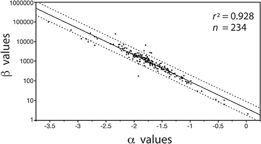
Figure 1. Bivariate plot (and regression statistics of the log-log normal curve) of the inverse autocorrelation between β vs. α values for the regressions of log₁₀-transformed stem diameter frequency distributions taking the general form of N_{{i, j}} = β_j log D${{}^{\left\{\mathit{\text{i}},\mathit{\text{j}}\right\}}}_{\text{α}\mathit{\text{j}}}$, where N is the number of stems in a bin size i and D is the diameter of the stems in the size bin i (see Niklas et al., 2003a). Dashed lines denote 95% CIs. The autocorrelation emerges because the measurement units of stem diameter is much smaller than the organisms being measured, i.e., the autocorrelation has no intrinsic biological meaning.

The goal of this paper is to explore the biological significance of β values drawing on examples from plant biology and evolution. In the following sections, we briefly review the historical background that prefaced the focus on scaling exponents to the neglect of their normalization constants. We then address the three major stumbling blocks concerning the interpretation of β values: (1) the units of β change according to the units of Y₁ and Y₂ when α ≠ 1.0, (2) β can only be computed in a size range for which the extrapolation of data is valid, and (3) β and α are often correlated (see Figure 1) simply because the units of measurement for Y₁ and Y₂ are much smaller than the size of the organs or organisms being measured. We show that in some cases the absolute value of β is biologically unimportant, whereas in other cases differences in β values illuminate biology. We conclude by offering suggestions for a research agenda focusing to elevate β to the equal status of α.

Preamble: Statistics and History

Before delving into the interpretation of β values, it is instructive to consider their “statistical” and “historical” background, i.e., why they emerge in the first place and why they are neglected in theoretical attempts to understand the biology of scaling.

Historical as well as recent studies show that researchers continue to debate the types of statistical models and the types of regression protocols that should be employed when investigating scaling relationships (Thompson, 1942; Sholl, 1950; Yates, 1950; Zuckerman, 1950; Gould, 1966; Smith, 1980; Harvey, 1982; Chappell, 1989; Packard, 2013). Nevertheless, there is consensus favoring linear regression when the error structure of a data set is multiplicative, heteroscedactic, and log normal, and the use of non-linear models when the error is additive, homoscedastic, and normal (Niklas and Hammond, 2014). The choice of model is not arbitrary therefore because (1) the error structure in a data set dictates the use of a linear or non-linear model and because (2) a data set cannot simultaneously manifest both error structures. Nevertheless, there are two philosophies regarding the implementation of a regression protocol, one that is strictly empirical and seeks the best fit to the data for the purpose of predicting trends, and another that emphasizes a mechanistic approach and seeks to test the predictions of a particular theory. In both cases, the classic scaling formula Y₁ = β Y${}_2^{\text{α}}$ can emerge, but the significance of its regression parameters differs according to the purpose of the analysis. When the purpose of regression analysis is prediction, the numerical values of β and α are strictly utilitarian. Indeed, a reviewer of Huxley's book, which arguably propelled the application of scaling analysis, noted that Huxley's methods were

…necessarily empirical. Of the causes of differential growth we have little knowledge; their investigation is the problem at issue. A variety of possible relations, in fact, reduce approximately to this formula. But it is not the object of the formula to establish the correctness of a particular hypothesis as the cause of differential growth; it merely expresses the observed facts with considerable accuracy in a simple way, so that many very significant features emerge which would not otherwise do so. (Pantin, 1932)

However, the objective of the modern analysis of scaling phenomena is to uncover the mechanisms that drive size-dependent changes in form. The numerical values of β and α are not just numbers plugged into an equation to predict the numerical value of a dependent variable based on the numerical value of its corresponding independent variable—the values of β and α can shed light why one variable changes in value as another changes in value.

Despite the dichotomy of how regression protocols are used, the disagreement about the importance of β values dates back to the seminal publications of Julian Huxley (1887–1975) and Georges Teissier (1900–1972) (Huxley and Teissier, 1936a,b). The two differed in opinion regarding the significance of β sufficiently enough that their simultaneously published articles—in English and French—differ by only one sentence, with Teissier endorsing the biological significance of β values (Huxley and Teissier, 1936a) and Huxley, by implication, dismissing their importance (Huxley and Teissier, 1936b).

This is in marked contrast with some the earliest scaling work done in the later 19th and early twentieth centuries. Early workers, such as the German Psychiatrist Otto Snell (1859–1939) and the Dutch paleontologist, geologist, and discoverer of “Java man” (Homo erectus) Eugene Dubois (1858–1940), attempted to derive a quantitative means of determining how “evolved” an organism was by comparing the mass of its brain to the mass of its body (Snell, 1892; Dubois, 1897). Dubois derived the formula

$\begin{array}{cc}\begin{array}{r}e=c{s}^r,\end{array}& (1)\end{array}$

or, when log-transformed,

$\begin{array}{cc}\begin{array}{r}log\mathit{\text{ e }}=logc+rlogs,\end{array}& (2)\end{array}$

where e (for encephalon) is brain size, c is the “coefficient of cephalization”, s is body size, and r is the “coefficient of relation” (Dubois, 1897). This same interest in correlating brain size with other traits, such as group size among primates, is a technique in practice 120 years later (Kudo and Dunbar, 2001).

Dubois' data would be combined with data on the brain sizes of various animals from diverse classes (reptilian, avis, and mammalia) by the French neuroscientist Louis Lapicque (1866–1952). Lapicque would present the data in 1907 by generating the first known log-log plot showing common slopes among allometric data (Lapicque, 1907) (Figure 2A). Curiously, Lapicque did not plot all of his data, perhaps because he thought of them as redundant (Figure 2B).

FIGURE 2

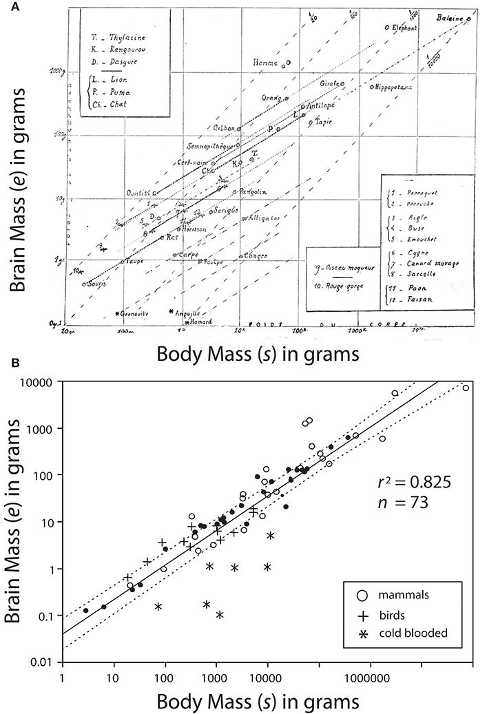
Figure 2. Bivariate plot of brain mass e vs. body mass s. (A) A photo-copy of the first known log-log plot showing common slopes among allometric data published by Louis Lapicque (1866–1952) in 1907. Dark dashed lines represent regression curves for individual species; gray dashed lines represent boundaries of interspecific trends. (B) Lapicque's data replotted to include data omitted from his original diagram. Missing data indicated by black circles. Reduced major axis regression curve and 95% CIs are provided.

During these initial studies, it was the magnitude of difference between the different organisms–what Dubois called the “coefficient of cephalization” (c) (Dubois, 1923, 1928), and what allometrists after Huxley and Tessier call the “normalization constant” (β)—that was the object of study. As noted by Gould's review of Dubois' later work:

“Dubois, 1922, Dubois (1928) built his famous theory of brain evolution on a belief that evolutionary increase in b [Gould used b in his notation instead of β] occurred in steps of a geometric progression with base 2. Thus, he reasoned, the brain evolves by a doubling of neurons early in embryology;(the change is reflected only in the increase of size- independent b; the slope remains constant)” Gould (1971)

That the scaling relationships between the mass of the brain and body seemed to have the same slope in log-log space was certainly an unusual observation, but it didn't forward the attempts to describe forms in terms of ratios of size, and it certainly didn't clarify how to quantify how “evolved” a given organism was.

Huxley's breakthrough, starting in 1924, was to focus on ratios of relative growth instead of ratios of size (Huxley, 1924). This began the shift in focus away from the differences in β, and with his joint 1936 paper with his Continental colleague, Teissier, firmly shifted the importance to α.

As a side note, we would be remiss if we failed to point out the historical timing and potential significance of the quotation with which we began this paper. Julian Huxley's younger brother, Aldous Huxley (1894–1962), published his novel Brave New World in 1931. This is firmly within the time period that the elder Huxley was deeply contemplating how to unify the Continental and English allometric literature, as they differed in both terminology and symbols used in equations. One can imagine the conversations between the two brothers, influencing one another in terminology and, by extension, the importance of variables (or people) as determined by the Greek letter used.

With the notable exception of Steven J. Gould's early work (White and Gould, 1965; Gould, 1966, 1967, 1971), the biological significance of β values has been largely as a side note to the more interesting α value (Newell, 1949; Huxley, 1950; Needham, 1950; Shadé, 1959). The lack of an underlying theory explaining the significance of β is strikingly similar to scaling theory before the emergence of the West, Brown, Enquist theory (West et al., 1997). This lack of attention is both a detriment to scaling theory and an immense opportunity for future research.

It would be ethically irresponsible when dealing with any historical treatment of allometry not to point out that the early application of scaling theory was often used to promote eugenics, racism, and anti-feminism (e.g., Snell, 1892). Clearly, this practice is totally unacceptable, intolerable, and scientifically invalid. As pointed out by Deacon (1990), the explicit assumption that brain size correlates in a positive linear or nonlinear way with intelligence has no valid scaling baseline for estimating differences in encephalization at different taxonomic levels. In addition, it conflates evolutionary trends in overall body and brain sizes with differences in cognitive abilities. Theories that purport to establish a correlation between brain size and intelligence are entirely incompatible with studies showing that intelligence is not intrinsically correlated with body size, but rather correlated with the degree of folding in the temporo-occiptal lobe, particularly in the outermost section of the posterior cingulate gyrus (Luders et al., 2008). And even these studies are inconclusive owing to other factors such as sexually dimorphic cranial features that conflate correlation with causation.

The Four Problems with β

As noted in the Introduction, there are three principal difficulties that have impeded the interpretation of β values and obscured their biological significance. Here, we address these three difficulties and show that they are avoidable and surmountable.

The Problem of Dimensionality

Unlike α, which is dimensionless and thus a “pure” number, β values have dimensionality. This is easily illustrated by a dimensional analysis of any allometric relationship as for example the scaling relationship between the critical bending height H_crit and basal stem diameter D of trees modeled as very slender columns:

$\begin{array}{cc}\begin{array}{r}{H}_{\text{crit}}=C{(\frac{E}{\rho g})}^{1/3}{D}^{2/3},\end{array}& (3)\end{array}$

or, when log-transformed and noting the constants in this equation,

$\begin{array}{cc}\begin{array}{r}log{H}_{\text{crit}}=(1/3)log\left[C(\frac{E}{\rho g})\right]+(2/3)LogD,\end{array}& (4)\end{array}$

where C is a dimensionless constant (approximately equal to 0.79 and 1.24 for an un-tapered and conical column, respectively), E is Young's elastic modulus (with units of N/m²), ρ is bulk tissue density (with units of kg/m³), and g is the gravitational constant (with units of m/s²) (Greenhill, 1881). When interpreted strictly as a scaling equation with the form Y₁ = β Y${{}^2}_{\text{α}}$, it follows that β is C(E/ρg)^1/3 and α is 2/3. Because N has units of kg m s⁻², dimensional analysis shows that β has units of m^1/3. Although this unit makes little biological sense, the importance of β cannot be rejected on dimensional grounds because any formula taking the form Y₁ = βY₂ ^α≠1 can be re-written as Y₁ = β₀ γ^1−α Y${{}^2}_{\text{α}}$, where γ is a dimensional conversion factor (a pacifier parameter) that has the same units as those used to measure Y₁ and Y₂. This conversion factor transforms β₀ into a dimensionless “pure” number equivalent to α regardless of the units used to measure Y₁ and Y₂. Although it is obvious, it bears repeating that Y₁ and Y₂ must be measured in the same units (e.g., m or kg) and that the units are applied to the same metric (e.g., body length or mass). Under these circumstances, comparisons are made among data sets using the same units of measurements, both β and β₀ have biological meaning. Provided that Y₁ and Y₂ are in the same units and the same metrics, we can set γ = 1 and continue to write Y₁ = β Y${}_2^{\text{α}}$, while recognizing that β is somewhat more complicated because it has units.

The issue of the units of measurement should not be overstated because there are mathematical tools to cope with using different units. It should be obvious that physical laws and biological phenomena cannot depend on the choice of units used to measure them. Thus, it should be equally obvious that scaling relationships between physical or biological quantities must be independent of the units in which they are measured. That this is so becomes evident by means of dimensional analysis as for example by the π-theorem. This theorem states that a physical relationship between a dimensional quantity and several parameters governing its relationship to them can be re-written as a relationship between a dimensional parameter and several dimensional products of the power of its governing parameters minus the number of governing parameters with independent dimensions. Barenblatt (2003) and Bridgman (1922) provide detailed and explicit expositions on the π-theorem and how it can be applied to scaling relationships.

To illustrate dimensional analysis, let us assume that cell growth G is some function of cell mass M and length L, and time T:

$\begin{array}{cc}\begin{array}{r}\mathit{\text{G}}=\mathit{\text{f}}(\mathit{\text{M}},\mathit{\text{L}},\mathit{\text{T}})\propto \mathit{\text{M}}{}^a\mathit{\text{L}}{}^b\mathit{\text{T}}{}^c,\end{array}& (5)\end{array}$

where the exponents a, b, and c are real numbers. The dimensional analysis of this formula proceeds by finding fixed relationships (proportionalities) between paired variables. For example, density ρ is the quotient of M and V. If cell cytosolic density is a constant, if follows that ρ = ML⁻³ = a constant, and assuming that cells increase in size without changing their geometry or shape, we see that V ∝ L³. Because M ∝ V, it follows that L ∝ M^1/3. Thus,

$\begin{array}{cc}\begin{array}{r}G\propto M^{a+b/3}{T}^c.\end{array}& (6)\end{array}$

Assuming that G depends on the rate at which mass is exchanged between a cell and its environment, G likely depends on overall metabolic rate, which has the dimensions of LT⁻¹. If this rate is constant on average, it follows that T ∝ L, and because L ∝ M^1/3, we find that T^c ∝ M^c/3 such that

$\begin{array}{cc}\begin{array}{r}\mathit{\text{G}}\propto M^{a+b/3+c/3}.\end{array}& (7)\end{array}$

This dimensional analysis is brought to closure when the dimensions of G are specified because the numerical values of a, b, and c depend on how Y₁ is measured. If G is measured as mass per unit time, G has the dimensions of MT⁻¹. Thus, the real numbers a, b, and c become 1, 0, and −1, respectively, such that G ∝ M^1+0/3−1/3 ∝ M^2/3. If G is measured as a production rate, which has units ML²T⁻³, we see that G ∝ M^1+2/3−3/3 ∝ M^0.333. This example shows that, for any formula Y₁ = βY${}_2^{\text{α}}$, the units of β and the numerical value of α depend on the numerical values of the real numbers a, b, and c, which depend in turn on the dimensions of Y₁ and Y₂.

The Range of Applicability Problem

The numerical value of β and α can change over the course of ontogeny and over the course of evolution. Therefore, β and α are not “constants” even for data sets gathered across similar species. This is strikingly evident when standing leaf dry mass per plant is plotted as a function of standing stem dry mass per plant for herbaceous plants, the juveniles of woody species, and mature individuals of woody species differing in age (Figure 3). Inspection of the resulting bivariant plot of data shows that the numerical values of β and α change in a statistically significant way once woody plant individuals begin to manifest secondary growth and accumulate wood in their stems. Among individuals of herbaceous species, the β value is numerically smaller and the α value is numerically higher than the corresponding values manifested by juvenile and mature plants belonging to woody species. The regression curves for these two plant groupings intersect at the point where secondary growth becomes anatomically evident in representative cross-sections through stems (the gray area in Figure 3). [In passing, this is also the size-range predicted by computer simulations in which tree species reach reproductive maturity (Hammond and Niklas, 2009)]. Importantly, in the absence of a careful understanding of plant anatomy and the phenomenology of secondary growth, the two regression curves would lead to significant errors in estimating standing leaf or standing stem dry mass (over estimating the former and under estimating the latter across woody plants).

FIGURE 3

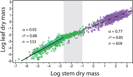
Figure 3. Bivariate plot of log₁₀-transformed standing leaf dry mass vs. standing stem dry mass (original units in kg) for herbaceous non-woody plants (green circles) and woody plants (purple triangles). The gray area in the middle of the plot denotes the region where the β and α values of the solid and dashed regression curves numerically change. This area also corresponds to where cross sections through representative stems manifest observable amounts of secondary tissues. Red dots indicate data from non-vascular and vascular seedless species (e.g., algae and mosses, and ferns and lycophytes). See text for scaling formulas. Data taken from the primary botanical literature.

This example illustrates an under-appreciated feature of any scaling analysis: it is not mathematically correct to present a formula such as Y₁ = β Y${}_2^{\text{α}}$ without specifying the range of Y₂ over which it holds true (i.e., Y_i ≤ Y₂ ≤ Y_j, where Y_i and Y_j are respectively the smallest and largest numerical values in a specified data set). Attempts to bypass this truism while giving β values biological meaning has resulted in meaningless mathematics, e.g., setting Y₂ equal to 1.0 at the lowest value in a data set such that Y₁ = β across all data sets (see Lumer et al., 1942). What is important is that β values have biological meaning over their stated Y_i ≤ Y₂ ≤ Y_j intervals even when Y_i > 1.0.

Extrapolating beyond the range of a data set is not necessarily a problem if the objective is to formulate predictions, or simply to graphically evaluate whether disconnected data share similar scaling exponents. Indeed, one of the efforts in science is to extend what we know to explain what we do not know. However, it is always important to know that range over which β- and α-values have been determined in scaling analyses.

The Inverse Relationship Problem

Figure 1 shows an inverse relationship between β and α values among a set [Y₁ = β Y${}_2^{\text{α}}$]. Similar inverse relationships have been reported by many early workers (e.g., Hersh, 1931; Hamai, 1938; Clark and Hersh, 1939; Anderson and Busch, 1941) so much so that the relationship β = a e^−bα (where a and b are constants) has been held to be biologically meaningful. That this is evidently not true is easily seen by asking under what conditions would we expect to see an inverse or direct correlation between β- and α-values and under what conditions would there be no correlation? The answer to this question can be obtained by hypothesizing a set of linear regression curves taking the form [Y₁ = β Y${}_2^{\text{α}}$] and by assuming that all of these curves intersect at one point (y₁, y₂), i.e., all of the curves share a common point defined by (y₁, y₂). Solving for the relationship between β and α, we obtain the formula

$\begin{array}{cc}\begin{array}{r}\text{β}={\text{β}}^{\prime }{({\mathit{\text{y}}}_2)}^{{\text{α}}^{\prime }-\alpha },\end{array}& (8)\end{array}$

where y${}_2^{\prime }$ is the numerical value of y₂ at the point of intersection and (β′, α′) is any ordered pair of the normalization constant and scaling exponent in the set of Y₁ = β Y${}_2^{\text{α}}$ regression curves (see White and Gould, 1965). Only three conditions exist for this formula (Figure 4): (1) when the point of intersection y${}_1^{\prime }$ is greater than one, an inverse correlation exists between β and α because β > β′ if and only if α′ > α, (2) when the point of intersection y${{}^1}_{\prime }$ equals one, β = β′ regardless of the value of α, and (3) when the point of intersection y${}_1^{\prime }$ is less than one, a direct correlation exists between β and α because β > β′ if and only if α > α′.

FIGURE 4

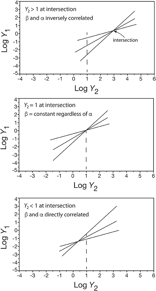
Figure 4. Three bivariate plots showing how the placement of a shared point of intersection in a set of log-log linear scaling relationships (only three are shown for convenience) affects whether β and α are inversely correlated (top), not correlated (middle), or directly correlated (bottom). See text for details.

The Detection Problem

Biologists often observe deviations in the linearity of log-log linear relationships spanning many orders of magnitude as in Figure 3 (e.g., Hammett and Hammett, 1939; Economos, 1983). In these cases, the challenge is to determine whether these deviations are statistically and biologically meaningful. From a strictly statistical perspective, determining whether the numerical value of β or α has changed can be detected using a variety of techniques as for example using segmented regression, change-point modeling, graphical inspection of regression residuals, and 95% confidence intervals (Quandt, 1958; Chow, 1960; Brown et al., 1975; Chappell, 1989). For example, Brown et al. (1975) developed the method of recursive residuals, which allows for a formal significance test. This method places considerable emphasis on graphical examination. Although a plot of residuals from a linear regression model is useful, it is not a very sensitive indicator of small changes in β. A more sensitive method was developed by Chappell (1989) that amounts to fitting a “bent line” by means of least squares regression protocols that can be validated subsequently by graphical diagnostics. Chappell's method provides a superior change-point regression model. However, it should be obvious that regardless of the technique used to determine whether the numerical value of β or α has changed presupposes that a researcher suspects that such has occurred. It is advisable, therefore, to test all scaling relationships to determine their log-log linearity.

Perhaps an even greater challenge is to determine whether a change in the numerical value of β or α is biologically meaningful. We are of the opinion that proof that a change is statistically significant is not a priori infallible proof that the change is biologically meaningful, and that the failure to detect a statistically significant change in a regression parameter does not necessarily mean that the change is biologically insignificant. A careful understanding of the biology of an organism or group of organisms provides the final arbitration of the challenging aspect of scaling analysis.

The Meaning of β

The four problems with β reviewed in the previous section obscure but do not diminish the biological significance of the normalization constant, which in many cases reflects an ontogenetic change in related organisms, or provides a descriptor of differences in growth or body type. Figure 3 provides an example of where a change in ontogeny (e.g., a shift from primary to secondary growth) is attended by significant changes in the numerical values of both β and α. Consider, another example showing how β values illuminate biology (i.e., the relationship between standing leaf dry mass, M_L, and standing stem dry mass, M_S) (Figure 5). Reduced major axis regression analyses of these data obtains M_L = 0.344 M${}_{\text{S}}^{0.751}$ for conifers and 0.132 M${}_{\text{S}}^{0.749}$ for angiosperms. In this example, the numerical values of the scaling exponents are statistically indistinguishable, whereas the β values significantly differ. Consequently, for any value of standing stem mass, the standing leaf mass of conifers is on average approximately 2.6 times larger than that of the angiosperms in this data set. This computation is mathematically trivial, but it exposes a biologically meaningful fact, viz coniferous species tend to retain their leaves (which tend to have high bulk tissue densities) for 2–3 years in contrast to angiosperms, the majority of which are deciduous.

FIGURE 5

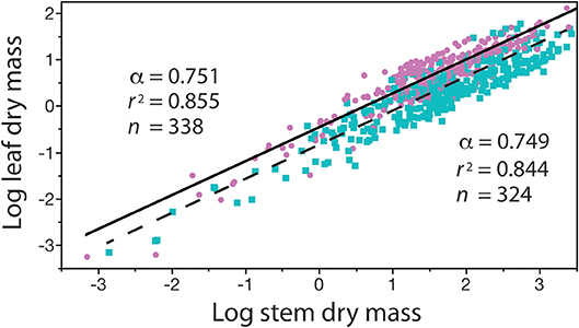
Figure 5. Bivariate plot (and regression parameters) of log₁₀-transformed standing leaf dry mass vs. standing stem dry mass (original units in kg) for conifers (purple circles) and angiosperms (blue squares) with corresponding solid and dashed regression curves. This example shows that differences in the numerical values of β indicate that, for any stem diameter, conifers bear more dry leaf mass than their angiosperm counterparts. See text for scaling formulas. Data taken from the Cannell (1982) worldwide compendium.

A third example in which β values take on importance is the relationship among the annual growth in stem, leaf, and root dry mass per plant: G_S, G_L, and G_R, respectively (Figure 6). Reduced major axis regression of the data shows that both G_S and G_R scale as the 1.14 power of G_L to yield the allometric formulas G_S = 1.64 G${}_{\text{L}}^{1.14}$ and G_R = 0.12 G${}_{\text{L}}^{1.14}$ (Table 1). These formulas hold across the herbaceous as well as arborescent species in the data set and indicate that on average both species groupings allocate an order of magnitude more of their total growth in body size to new stem tissues as opposed to new root tissues. This is probably a gross over-estimate because the data for root dry mass are skewed for woody roots rather than new feeder roots. Nevertheless, estimates indicate that stem growth exceeds that of total root growth.

FIGURE 6

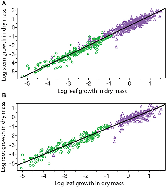
Figure 6. Bivariate plots of log₁₀-transformed data for stem, leaf, and root annual growth rates (original units stranding dry mass produced per year per plant) for herbaceous non-woody (green circles) and woody (purple triangles) species. Solid lines are log-log regression curves. (A) Stem growth vs. leaf growth. (B) Root growth vs. leaf growth. See text and Table 1 for scaling formulas and regression parameters. Data for herbaceous species taken from the primary botanical literature; data for woody species taken from the Cannell (1982) worldwide compendium.

TABLE 1

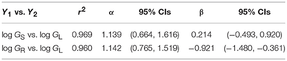
Table 1. Reduced major axis regression parameters for the scaling of annual growth in stem, leaf, and root dry mass (G_S, G_L, and G_R, respectively) per plant per year (log₁₀-transformed data plotted in Figure 5). Original units kg/yr.

Yet another example illustrating the importance of β values is their role in understanding plant size frequency distributions, species richness, and species-specific density. For example, across the data sets accumulated by Alwyn H. Gentry (1945–1993), stem size frequency distributions are approximated by the formula N_i = β Log D${}_{\text{i}}^{\text{α}}$, where N_i is the number of individuals within stem diameter D_i bin size (Enquist and Niklas, 2001; Niklas et al., 2003a). However, the numerical values of β and α change as a function of any change in bin size, Δx. Mathematical analyses of this variation obtains a formula predicting the total number of individuals in any size frequency distribution, N_T, approximated by the formula N_i = β log D${}_{\text{i}}^{\text{α}}$ as a function of β, α, Δx, and maximum and minimum stem diameter (Niklas et al., 2013b):

$\begin{array}{cc}\begin{array}{r}{N}_T=\frac{\beta }{\Delta x(1-\alpha )}(D_{max}^{1-\alpha }-D_{min}^{1-\alpha }).\end{array}& (9)\end{array}$

The importance of β in this context is mathematically transparent because it equals the quotient of the number of individuals in the smallest bin size Δx_min and D_min^α (i.e., β = Δx_min / D_min^α), a relationship that obviates the autocorrelation between β and α (see Figure 1) in subsequent analyses of the biological significance of size frequency distributions (Niklas et al., 2013b).

β in Development and Evolution

The significance of β values in development and evolution can be seen in the context of how organic shape might change in an ancestor-descendent transition. Consider a log-log plot of the size of one organ-type Y₁ against another organ-type Y₂ (Figure 7). In the isometric condition (i.e., Y₁ = β Y${}_2^{\text{α}=1}$), it follows that β = Y₁/Y₂, which is dimensionless and thus can serve as a measure of shape if Y₁ and Y₂ are metrics of form (e.g., petal length and sepal length). In this example, β is invariant and the organism does not change its shape throughout its ontogeny (Figure 7A). If this type of organism gives rise to a descendent for which the relationship between Y₁ and Y₂ is allometric (i.e., α ≠ 1), it is evident that shape has changed and that it changes allometrically throughout the ontogeny of the descendent (i.e., β = Y₁/Y${}_2^{\text{α}}$). Consequently, changes in β values in the phylogeny of a lineage or clade can be used to infer evolutionary changes in shape or some other variable of interest. This hypothetical scenario is not unlike the evolutionary transition between plants capable only of primary growth into those capable of secondary growth (as reflected in Figure 3).

FIGURE 7

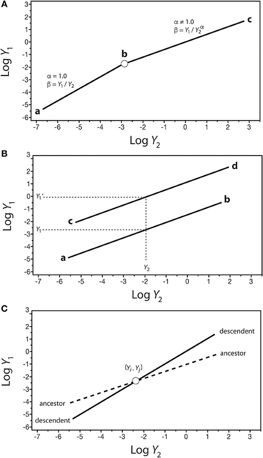
Figure 7. Hypothetical scaling relationships between two body parts, Y₁ and Y₂, showing changes in β–values over the course of development or evolution. (A) The shift between an ancestral isometric scaling relationship between Y₁ and Y₂ (denoted by the line a-b) and an allometric relationship in the descendent (denoted by the line b-c). (B) Two scaling relationships sharing the scaling exponent (denoted by lines a-b and c-d) but differing in β values. For any value of Y₂, there exist two corresponding values of Y₁ (i.e., Y₁ and Y₁'). (C) An ancestor-descendent relationship (denoted by dashed and solid lines, respectively) in which β and α values change. If the ancestral body shape achieved at point (Y_i, Y_j) occurs earlier in the ontogeny of the descendent, development has accelerated. If the ancestral body shape achieved at point (Y_i, Y_j) occurs later in the ontogeny of the descendent, development has been retarded.

Comparisons of shape are possible even when Y₁ vs. Y₂ is allometric (i.e., α ≠ 1), provided that scaling relationships share the same exponents. Consider two regressions with the same α values: Y₁ = β₁Y${}_2^{\text{α}}$ and Y₁' = β₁${\mathrm{Y\prime }}_2^{\text{α}}$ (Figure 6B). For any value of Y₂ within the range of both regression curves, there are two values of Y₁ (i.e., at Y₂, Y₁ ≠ Y${}_1^{\prime }$), such that β₁/β₂ = (Y₁/ Y${}_2^{\text{α}}$) / (Y${}_1^{\prime }$/ Y${}_2^{\text{α}}$) = Y₁/ Y${}_1^{\prime }$. This relationship can be used to consider what appear to be stepwise (saltational) ancestor-descendent differences between related organisms (as reflected in Figure 5).

Finally, consider the case of two regression curves, Y₁ = β₁$Y_2^{\text{α}}$ and ${\mathrm{Y\prime }}_1={\beta }_2$ ${\mathrm{Y\prime }}_2^{\text{α}}$, that intersect at a single point, (Y_i, Y_j), such that ${\mathrm{Y\prime }}_1$ < Y′₁ below the intersection point and $Y_1>{\mathit{\text{Y}}}_1$ above the intersection of the two curves (Figure 7C). Under these conditions, it follows that (β₁/β₂) = Y_j ^(α′−α), or Y_j = (β₁/β₂)^{1/(α′−α)}. This relationship can be used to compare ancestor-descendent ontogenies as to when the form specified by the metrics (Y_i, Y_j) is achieved during growth. If the descendent achieves (Y_i, Y_j) earlier than the ancestor, the ontogenetic trajectory of the descendent has been accelerated with respect to that of the ancestor, as shown in Figure 7C. If the descendent achieves (Y_i, Y_j) later than the ancestor, the ontogenetic trajectory of the descendent has been retarded with respect to that of the ancestor. Note that (1) the terms “earlier,” “accelerated,” and “retarded” refer to rates of change, specifically the rate of change of Y₁ with respect to Y₁, i.e., ∂Y₁/∂Y₂ = β₁(α)Y${}_2^{\text{α}-1}$ and ∂Y${}_1^{\prime }/\partial$ Y${}_2^{\prime }={\beta }_2({\alpha }^{\prime }$)${\mathrm{Y\alpha \prime -1}}_2$, and (2) the point (Y_i, Y_j) represents some designated shared stage in the ontogeny of the ancestor and descendent (e.g., the time of germination, or sexual maturity).

Future Directions

The purpose of this review was to show that β values are as biologically meaningful as α. That this is so becomes immediately apparent because, in general terms, β is dimensionless (i.e., a “pure” number) dependent on the scale used to measure the relationship between two variables of interest, i.e., β = Y₁/Y₂ when α = 1 and β = Y₁ / (γ^1−α Y₂ ^α) when α ≠ 1 (where γ is a dimensional conversion factor). Yet, despite its obvious importance, little attention has been paid to how or why β values differ across data sets or lineages, or how it changes during the course of evolution by natural selection.

Future studies can, at the very least, document how β values relate to the scaling exponents governing the relationships being investigated. The greater challenge is to explain why β values differ and what these changes mean. A good way to approach this challenge is to first explore isometric scaling relationships. For example, using a large data set reporting the annual production (growth) of new leaves and stems, G_L and G_S, across conifer and angiosperm tree species (Cannell, 1982), Niklas and Enquist (2002) found an isometric scaling relationship such that β = G_L/G_S. Because G_L is the product of the number of new leaves produced per year, n_L, and leaf area, thickness, and bulk tissue density (A_L, t, and ρ_L) because G_S is the product of the number of new stems produced per year, n_S, and stem length, transverse area, and bulk tissue density (L, A_S, and ρ_L), it follows that β = (n_L A_L t ρ_L)/(n_S L A_S ρ_S) across species. Assuming that the average values of A_L, t, L, A_S, ρ_L and ρ_S are invariant for any particular species, we see that in theory β describes the intraspecific proportional relationship between the number of new leaves and stems produced per plant per year, i.e., β ∝ (n_L/n_S). Thus, if the numerical value of β remains constant for a particular species, it follows that the number of new leaves produced per year remains proportional to the number as well as the size of new stems produced per year over the course of a plant's ontogeny. This scenario is not biologically unreasonable because the number of leaves on twigs is likely to be proportional to the size of the stems bearing them. Regardless, the hypothesis engendered by considering β to be biologically meaningful is testable empirically.

In a broader sense, what we are proposing is the examination if β in terms of trait-based ecology. Far from being a modern point of interest, trait-based ecology can be traced back to Theophrastus' Enquiry into Plants (Περi $\varphi \upsilon \tau \tilde{\omega }\nu$ iστoρiα) written between 350 and 287 BCE, wherein he classified plants as trees, shrubs, or grasses based primarily on height and stem density (Morton, 1981) While these general traits have remained as major de facto classifications for terrestrial plants, ecologists have continued to propose additional trait-based criteria (for reviews, see Weiher et al., 1999; Westoby et al., 2002). The interest in conducting research in trait-based ecology is the underlying belief that understanding trait costs and benefits will provide insights into how vegetation properties differ over space (geography) and time (evolution), and explain patterns of diversity (MacArthur, 1984; Messier et al., 2010).

Part of what we have tried to illustrate in this paper is that β can often be a measure of differences in a quantitative trait among species or within a species. Real and meaningful trait-based differences between conifers and angiosperms in terms of their standing leaf mass relative to the standing stem mass can be seen when examining the numerical values of the β values (Figure 4). Differences in β should not be limited to what one sees among species, however: within the same species one should predict to see statistically identical α values, but differing β values depending on the natural variation of the environment. Soil quality, light intensity, water availability, and a host of other environmental factors should all contribute to intra-species variation in β that is measurable and meaningful, beyond the inter-species variations in β. Put another way, inter-species variations in β reflect different evolutionary strategies, whereas intra-species variations in β reflect the limits of the species' plasticity to environmental variation.

We are certainly not the first to propose the importance of β in terms of trait-based ecology. Work by Brian Enquist, for example, illustrated how the β for the annual biomass growth vs. whole plant leaf biomass could be derived for angiosperms and gymnosperms (Enquist et al., 2007). The paucity of published work related to β as being biologically meaningful strengthens our sense that this line of inquiry remains under-researched, and can potentially offer important insights into the questions of ecological trait-based fitness, natural plasticity, and evolutionary/biogeographical history.

Author Contributions

KN and SH wrote the paper and prepared the figures.

Conflict of Interest Statement

The authors declare that the research was conducted in the absence of any commercial or financial relationships that could be construed as a potential conflict of interest.

Acknowledgments

The authors thank Drs. Mary O'Connor, Angélica L. González, Diego Barneche, and Julie Messier who as editors of this special issue of Frontiers of Ecology and Evolution invited this contribution. They also thank Drs. Randy Wayne and Thomas Owens (Cornell University) and the Drs. Brummer, Michaletz, and Savage who gave generously of their time and for their constructive comments on an early draft of this paper. Funding from the College of Agriculture and Life Science (to KN) is also gratefully acknowledged.

References

Anderson, B. G., and Busch, H. L. (1941). Allometry in normal and regenerating antennal segments in Daphnia. Biol. Bull. 81, 119–126. doi: 10.2307/1537626

CrossRef Full Text | Google Scholar

Barenblatt, G. I. (2003). Scaling. Cambridge: Cambridge University Press. doi: 10.1017/CBO9780511814921

CrossRef Full Text | Google Scholar

Bridgman, P. W. (1922). Dimensional Analysis. New Haven, CT: Yale University Press.

Brown, R. L., Durbin, J., and Evens, J. M. (1975). Techniques for investigating the constancy of regression relationships over time (with Discussion). J. R. Stat. Soc. B 37, 149–192.

Cannell, M. G. R. (1982). World Forest Biomass and Primary Production Data. New York: Academic Press.

Google Scholar

Chappell, R. (1989). Fitting bent lines to data, with applications to allometry. J. Theor. Biol. 138, 235–256. doi: 10.1016/S0022-5193(89)80141-9

PubMed Abstract | CrossRef Full Text | Google Scholar

Chow, G. (1960). Tests of equality between two sets of coefficients in two linear regressions. Econometrika 28, 561–605. doi: 10.2307/1910133

CrossRef Full Text

Clark, L. B., and Hersh, A. H. (1939). A study of relative growth in Notonecta undulata. Growth 3, 7–372.

Deacon, T. W. (1990). Fallacies of progression in theories of brain-size evolution. Int. J. Primatol. 11, 193–236. doi: 10.1007/BF02192869

CrossRef Full Text | Google Scholar

Dubois, E. (1897). Sur le rapport du poids de l'encéphale avec la grandeur du corps chez les mammifères. bmsap 8, 337–376. doi: 10.3406/bmsap.1897.5705

CrossRef Full Text | Google Scholar

Dubois, E. (1923). Phylogenetic and ontogenetic increase of the volume of the brain in vertebrata. Proc. Koninklijke Nederlandse Akad. Wetenschappen 25, 230–255.

Dubois, E. (1928). The law of necessary phylogenetic perfection of the psychoencephalon. Proc. Sec. Sci. Akad. Wetenschappen Amsterdam 31, 304–314.

Economos, A. C. (1983). Elastic and/or geometric similarity in mammalian design? J. Theor. Biol. 103, 167–172. doi: 10.1016/0022-5193(83)90206-0

PubMed Abstract | CrossRef Full Text | Google Scholar

Enquist, B. J., Kerkhoff, A. J., Stark, S. C., Swenson, N. G., and Price, C. A. (2007). A general integrative model for the scaling plant growth, carbon flux, and functional trait spectra. Nature 449, 218–222. doi: 10.1038/nature06061

PubMed Abstract | CrossRef Full Text | Google Scholar

Enquist, B. J., and Niklas, K. J. (2001). Invariant scaling relation across tree-dominated communities. Nature 410, 655–660. doi: 10.1038/35070500

CrossRef Full Text | Google Scholar

Gould, S. J. (1966). Allometry and size in ontogeny and phylogeny. Biol. Rev. Camb. Philos. Soc. 41, 587–640. doi: 10.1111/j.1469-185X.1966.tb01624.x

PubMed Abstract | CrossRef Full Text | Google Scholar

Gould, S. J. (1967). Ontogeny and Phylogeny. Cambridge, MA: Belknap Press.

Google Scholar

Gould, S. J. (1971). Geometric similarity in allometric growth: a contribution to the problem of scaling in the evolution of size. Am. Nat. 105, 113–136. doi: 10.1086/282710

CrossRef Full Text | Google Scholar

Greenhill, A. G. (1881). Determination of the greatest height consistent with stability that a vertical pole or mast can be made, and of the greatest height to which a tree of given proportions can grow. Proc. Camb. Philos. Soc. 4, 65–73.

Hamai, I. (1938). Some notes on relative growth with special reference to the growth of limpets. Sci. Rep. Tohoku Univ. 12, 71–95.

Hammett, F. S., and Hammett, D. W. (1939). Proportional length growth in Gar. Growth 31, 197–209.

Hammond, S. T., and Niklas, K. J. (2009). Emergent properties of plants competing in silico for space and light: seeing the tree from the forest. Am. J. Bot. 98, 1430–1444. doi: 10.3732/ajb.0900063

CrossRef Full Text | Google Scholar

Harvey, P. H. (1982). On rethinking allometry. J. Theor. Biol. 95, 37–41. doi: 10.1016/0022-5193(82)90285-5

PubMed Abstract | CrossRef Full Text | Google Scholar

Hersh, A. H. (1931). Facet number and genetic growth constants in bar eyed stocks of Drosophila. J. Exp. Zool. 60, 213–248. doi: 10.1002/jez.1400600204

CrossRef Full Text | Google Scholar

Huxley, J. S. (1924). Constant differential growth-ratios and their significance. Nature 114, 895–896. doi: 10.1038/114895a0

CrossRef Full Text | Google Scholar

Huxley, J. S. (1950). A discussion on the measurement of growth and form; relative growth and form transformation. Proc. R. Soc. Lond. Ser. B Biol. Sci. 137, 465–469. doi: 10.1098/rspb.1950.0055

PubMed Abstract | CrossRef Full Text | Google Scholar

Huxley, J. S., and Teissier, G. (1936a). Terminologie et notation dans la description de la croissance relative. Comptes Rendus Séances Soc. Biol. ses filiales 121, 934–936.

Huxley, J. S., and Teissier, G. (1936b). Terminology of relative growth. Nature 137, 780–781. doi: 10.1038/137780b0

CrossRef Full Text | Google Scholar

Kudo, H., and Dunbar, R. I. M. (2001). Neocortex size and social network size in primates. Anim. Behav. 62, 711–722. doi: 10.1006/anbe.2001.1808

CrossRef Full Text | Google Scholar

Lapicque, L. (1907). Tableau général des Poids somatique et encéphalique dans les espèces animales. Bull.Mémoires Soc.d'Anthropol. Paris 8, 248–270. doi: 10.3406/bmsap.1907.7004

CrossRef Full Text | Google Scholar

Luders, E., Narr, K. L., Bilder, R. M., Szeszko, P. R., Gurbani, M. N., Hamilton, L., et al. (2008). Mapping the relationship between cortical coevolution and intelligence: effects of gender. Cereb. Cortex 18, 2019–2026. doi: 10.1093/cercor/bhm227

PubMed Abstract | CrossRef Full Text | Google Scholar

Lumer, H., Anderson, B. G., and Hersh, A. H. (1942). On the significance of the constant b in the law of allometry. Am. Nat. 76, 364–375. doi: 10.1086/281053

CrossRef Full Text | Google Scholar

MacArthur, R. H. (1984). Geographical Ecology: Patterns in the Distribution of Species. Princeton, NJ: Princeton University

Google Scholar

Messier, J., McGill, B. J., and Lechowicz, M. J. (2010). How do traits vary across ecological scales? A case for trait-based ecology. Ecol. Lett. 13, 838–848. doi: 10.1111/j.1461-0248.2010.01476.x

PubMed Abstract | CrossRef Full Text | Google Scholar

Morton, A. G. (1981). History of Botanical Science. An Account of the Development of Botany from Ancient Times to the Present Day. New York, NY: Academic Press.

Google Scholar

Needham, J. (1950). Biochemistry and Morphogenesis. Cambridge: Cambridge University Press.

Google Scholar

Newell, N. D. (1949). Phyletic size increase, an important trend illustrated by fossil invertebrates. Evolution 3, 103–124. doi: 10.1111/j.1558-5646.1949.tb00010.x

PubMed Abstract | CrossRef Full Text | Google Scholar

Niklas, K. J., and Enquist, B. J. (2002). On the vegetative biomass partitioning of seed plant leaves, stems, and roots. Am. Nat. 159, 482–497. doi: 10.1086/339459

PubMed Abstract | CrossRef Full Text | Google Scholar

Niklas, K. J., and Hammond, S. T. (2014). Assessing scaling relationships: uses, abuses, and alternatives. Int. J. Plant Sci. 175, 754–763. doi: 10.1086/677238

CrossRef Full Text | Google Scholar

Niklas, K. J., Midgley, J. J., and Rand, R. H. (2003a). Tree size frequency distributions, plant density, age, and community disturbance. Ecol. Lett. 6, 405–411. doi: 10.1046/j.1461-0248.2003.00440.x

CrossRef Full Text | Google Scholar

Niklas, K. J., Midgley, J. J., Rand, R. H., and Packard, G. C. (2013b). Size-dependent species richness: trends within plant communities and across latitude. Ecol. Lett. 6, 631–636. doi: 10.1046/j.1461-0248.2003.00473.x

CrossRef Full Text | Google Scholar

Packard, G. C. (2013). Is logarithmic transformation necessary in allometry? Biol. J. Linnean Soc. 109, 476–486. doi: 10.1111/bij.12038

CrossRef Full Text | Google Scholar

Pantin, C. (1932). Form and size. Nature 129, 775–777. doi: 10.1038/129775a0

Quandt, R. E. (1958). The estimation of the parameters of a liner regression system obeying two separate regimes. J. Am. Stat. Assoc. 53, 873–880. doi: 10.1080/01621459.1958.10501484

CrossRef Full Text | Google Scholar

Shadé, J. P. (1959). Differential growth of nerve cells in cerebral cortex. Growth 23, 159–168.

PubMed Abstract | Google Scholar

Sholl, D. A. (1950). The theory of differential growth analysis. Proc. R. Soc. Lond. Ser. B Biol. Sci. 137, 470–474. doi: 10.1098/rspb.1950.0056

PubMed Abstract | CrossRef Full Text | Google Scholar

Smith, R. (1980). Rethinking allometry. J. Theor. Biol. 87, 97–111. doi: 10.1016/0022-5193(80)90222-2

PubMed Abstract | CrossRef Full Text | Google Scholar

Snell, O. (1892). Die Abhangigkeit des Hirngewichtes von dem Korpergewicht und den geistigen Fahigkeiten. Eur. Arch. Psychiatry Clin. Neurosci. 23, 436–446. doi: 10.1007/BF01843462

CrossRef Full Text | Google Scholar

Thompson, D. W. (1942). On Growth and Form. Cambridge: Cambridge University Press.

Google Scholar

Weiher, E., van der Werf, A., Thompson, K., Roderick, M., Garnier, E., and Eriksson, O. (1999). Challenging theophrastus: a common core list of plant traits for functional ecology. J. Veg. Sci. 10, 609–620. doi: 10.2307/3237076

CrossRef Full Text | Google Scholar

West, G. B., Brown, J. H., and Enquist, B. J. (1997). A general model for the origin of allometric scaling laws in biology. Science 276, 122. doi: 10.1126/science.276.5309.122

PubMed Abstract | CrossRef Full Text | Google Scholar

Westoby, M., Falster, D. S., Moles, A. T., Vesk, P. A., and Wright, I. J. (2002). Plant ecological strategies: some leading dimensions of variation between species. Annu. Rev. Ecol. Syst. 33, 125–159. doi: 10.1146/annurev.ecolsys.33.010802.150452

CrossRef Full Text | Google Scholar

White, J., and Gould, S. (1965). Interpretation of the coefficient in the allometric equation. Am. Nat. 99, 5–18. doi: 10.1086/282344

CrossRef Full Text | Google Scholar

Yates, F. (1950). The place of statistics in the study of growth and form. Proc. R. Soc. Lond. Ser. B Biol. Sci. 137, 479–488. doi: 10.1098/rspb.1950.0058

PubMed Abstract | CrossRef Full Text | Google Scholar

Zuckerman, S. (1950). The pattern of change in size and shape. Proc. R. Soc. Lond. Ser. B Biol. Sci. 137, 433–443. doi: 10.1098/rspb.1950.0051

PubMed Abstract | CrossRef Full Text | Google Scholar