Spatiotemporal Heterogeneity of Water Flowpaths Controls Dissolved Organic Carbon Sourcing in a Snow-Dominated, Headwater Catchment

Introduction

In mountainous headwater catchments, snow is often the dominant phase of precipitation (Barnett and Adam, 2005) and snowpacks act as reservoirs, storing water from winter storms and releasing it later, often sustaining streamflow through the growing season at downstream locations (Williams et al., 2002; Nayak et al., 2010). Thus, streamflow and the processes it influences often depend on the transition between snow and rain (Marks et al., 2013). The range of elevations over which this transition occurs is known as the rain-snow transition, and although its location can shift between and during storm events, it commonly has a characteristic range of elevations in a given geographic region (Marks et al., 2013; Klos et al., 2014). One major impact of climate change is an upward shift in the elevation of the rain-snow transition, which affects snowpack size and location (Klos et al., 2014; Tennant et al., 2017). In turn, the different hydrologic responses of a given basin to rain vs. snow will affect streamflow and groundwater supplies (Marks et al., 2013).

Snowmelt and snowdrifts dominate the hydrology of mountain regions around the world (Viviroli et al., 2007). Snowdrifts are created by the interaction of wind and topography, as wind removes snow from exposed areas and drops it on lee slopes (Winstral and Marks, 2002). This amounts to “drift” (accumulation) areas receiving a precipitation subsidy from “scour” (removal) areas (Winstral and Marks, 2014). Drifts tend to form in the same locations annually (visible with LiDAR data, remotely sensed imagery, or via field observations), resulting in greater spatial heterogeneity of precipitation in snowdrift-dominated catchments than in those where drifting does not occur (Grünewald et al., 2010; Sturm and Wagner, 2010; Winstral and Marks, 2014). This impacts hydrologic flowpaths in these systems (Pomeroy et al., 2007).

Hydrologic flowpaths are constrained by topography, soil and bedrock porosity, and evapotranspiration (Soulsby et al., 2006; Tetzlaff et al., 2007). In a system with several large upstream snowdrifts and only one stream, meltwater that does not evaporate or sublimate from the drift surface must flow downhill into the stream from the melting drifts, unless it is lost to deep regional aquifers. While stream water is likely derived predominantly from the drift, a key question is how water gets to the stream. What does it flow through? How long does it take? What solutes does it acquire en route?

If snowdrifts can be considered aboveground “water towers” in mountainous systems (Viviroli et al., 2007), then aquifers can be thought of as belowground “storage tanks.” Bedrock aquifers, where present, are considered the major source of stream baseflow during periods of little precipitation (Dingman, 2015). In snow-dominated systems, it is common for snowmelt to be the dominant aquifer-recharge event (Fleckenstein et al., 2006; Seyfried et al., 2009). Water from the drifts infiltrates through the soil, where soil is present in the catchment, dissolving minerals and organic material from the soil matrix (Lohse et al., 2009). The water may recharge the bedrock aquifer, or it may run along the bedrock/soil interface into the stream (Stieglitz et al., 2003). The paths water follows affect the species and quantity of solutes it carries.

After the initial pulse of snowmelt, snow-dominated watersheds may begin to dry out from the ridgetops down (Stieglitz et al., 2003). In drier areas, soil water continues to accumulate solutes, but this water will not reach the stream until sufficient hydrologic connectivity is restored through soil saturation (Stieglitz et al., 2003; Sanderman et al., 2009; Stielstra et al., 2015; Li et al., 2017). Since hydrologic connectivity is not uniform across most catchments, patterns in solute concentration in stream waters will be influenced by patterns in connectivity (Li et al., 2017).

Dissolved organic carbon (DOC) is a solute of particular interest because it is the most mobile form of carbon and plays an important role in the global carbon (C) cycle. In headwater catchments, especially those where subsurface flow predominates, the primary source of DOC is soil organic carbon (SOC) leached by precipitation and carried to the stream (Boyer et al., 1997). DOC is an important component of aquatic food webs, while SOC in the form of soil organic matter (SOM) increases the availability of water and nutrients for plant growth (Doran, 2002; Cole et al., 2007; Crimmins et al., 2011). Loss of SOM can reduce soil fertility, while much of the SOC lost to rivers is eventually respired to the atmosphere in the form of carbon gasses such as carbon dioxide and methane (Doran, 2002; Cole et al., 2007).

Climate change has the potential to cause particularly large changes in mountainous regions, including altering the level of the rain-snow transition, and the proportions of rain and snow on an annual basis (Beniston, 2003; Klos et al., 2014; Tennant et al., 2017). Changes in the proportions of rain and snow in a catchment can impact hydrologic flowpaths; and insofar as hydrology affects carbon transport, these changes can also impact the export of DOC from mountainous headwater catchments (Boyer et al., 1997; Jones et al., 2005). Rising atmospheric concentrations of methane and carbon dioxide in the past few centuries have already altered global climate, affecting temperature and water availability worldwide (Intergovernmental Panel on Climate Change., 2014). The stability of SOM is influenced by temperature and water availability, and as SOM represents a major store of carbon worldwide, there exists a potential feedback loop—climate change leading to greater release of soil carbon, which then changes the climate further (Eswaran et al., 1993; Zogg et al., 1997; Cox et al., 2000; Jones et al., 2005).

At the intersection of snow hydrology and carbon export is the “flushing” hypothesis (Boyer et al., 1997). While the snowpack remains frozen, only limited export of soil water occurs, and soil pore waters accumulate solutes, including DOC. In spring, snowmelt flushes this concentrated soil water into the stream, along with the solutes it carries. This is a major control on soil carbon export and stream DOC dynamics (e.g., Hornberger et al., 1994; Boyer et al., 1997; Hood et al., 2006). Studies of carbon export commonly use the relative abundance of complex carbon molecules (lignins, tannins, etc.) as an indicator of carbon sourcing (Wickland et al., 2007). While this provides valuable insight into the ultimate sources of DOC (e.g., Neff et al., 2006; Lapworth et al., 2008), it can become problematic if carbon is used to trace water flowpaths (e.g., Fiebig et al., 1990; Boyer et al., 1997), because it assumes that soil water is the primary source of water generating streamflow, and therefore that SOC is the primary source of DOC. In order to examine this assumption, we quantify and characterize DOC in the stream and potential source waters, develop an end-member mixing model using more conservative, inorganic tracers, and then use the fractional water contributions derived from the model to predict stream DOC based on the DOC concentration of source waters. Comparing modeled DOC from water contributions to measured DOC in the stream—combined with DOC characteristics—allows us to disentangle the interactions between soil carbon, soil water, and deeper flowpaths in the watershed.

In this study, we explore how the hydrologic dynamics of snow-dominated watersheds interact with carbon stores to affect stream carbon export, specifically:

1. What paths does meltwater from seasonal snowdrifts follow on its way to the stream?

2. Is soil water a major component of the hydrograph in drift-dominated systems, or is carbon being brought into the stream by another subsurface flowpath?

3. What are the patterns of DOC concentrations in stream and source waters? Do they follow the “flushing” model, or is there another factor driving carbon export?

To address these questions, we sampled all likely end-members (soil water, saprolite water, deeper groundwater, rain, and snow) and compared their cation and anion concentrations to those in stream water to determine the flow paths in this watershed. To determine hydrologic response, we measured soil moisture and matric potentials in three soil pits at three depths; depth to water table in wells drilled in the bedrock aquifer; and isotopic composition of waters taken from soil, saprolite, bedrock, snowpack, rainfall, and stream. These likely end-members were quantified using end-member mixing analysis (EMMA) and a mixing model was used to indicate the primary sources of stream flow. We compared the relative contributions of carbon and water to the stream by each end-member to evaluate which flowpath was contributing most of the DOC to the stream, and we determined the most likely source of DOC using the specific ultraviolet absorbance (SUVA) and fluorescence index (FI) of carbon from stream water and end-member samples.

Materials and Methods

Site Description

Reynolds Mountain East (RME) is a 0.38 km² headwater catchment in the Reynolds Creek Experimental Watershed (RCEW)/Reynolds Creek Critical Zone Observatory (RC-CZO) in the Owhyee Range in southwestern Idaho, USA (Figure 1A). The catchment ranges from 2,020 to 2,140 m in elevation over an area of 0.38 km²; slopes vary from 0 to 40% (Seyfried et al., 2009). RME has been intensively monitored as a United States Department of Agriculture Agricultural Research Service (USDA-ARS) experimental watershed for over 50 years (e.g., Marks et al., 2001; Flerchinger et al., 2010; Reba et al., 2011; Winstral and Marks, 2014), and as a National Science Foundation Critical Zone Observatory for the past 5 years.

FIGURE 1

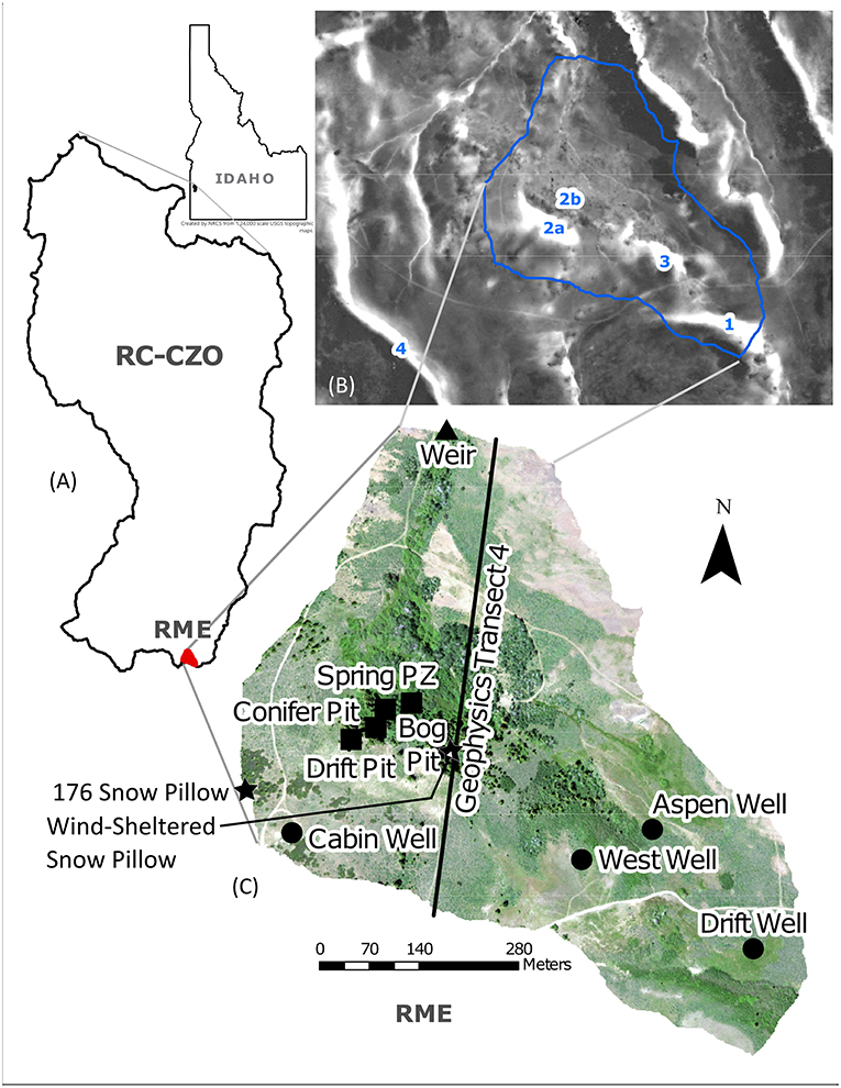
Figure 1. (A) The Reynolds Mountain East (RME) catchment is located in southwestern Idaho, USA, at the southern end of the Reynolds Creek CZO. (B) Snowdrifts in RME are highlighted by a snow depth map from March 2009 (an average snow year) with white areas indicating drifts marked by numbers 1, 2a&b, 3, and 4 referenced in the main text. Snow depth data from Shrestha (2016). (C) Annotated RME orthophoto outlines instrument and sampling locations. 176 is the “exposed ridge” meteorology station and Judd snow-depth site; the “wind-sheltered” snow pillow is directly in line with the geophysics transect. “PZ” stands for piezometer, which is co-located with the soil moisture and matric-potential probes at each pit.

RME receives ~900 mm of precipitation annually, of which more than 70% is delivered in the form of snow, and exports ~520 mm of this as stream flow (Seyfried et al., 2009). Snow commonly accumulates in deep (>2 m) drifts in sheltered areas (Winstral and Marks, 2014). One large drift, the East drift, forms at the eastern end of the catchment, on the leeward side of an unnamed peak (Figure 1B, No. 1). A smaller drift forms at the base of the steep hill below the cabin (Figure 1B, No. 2); little to no drifting occurs in the Douglas-fir forest below this drift, but in exceptionally snowy years, a smaller drift forms downhill of the Douglas firs (Figure 1B, No. 2b). Another drift forms just east of this drift, downhill of the East drift, in an aspen stand (Figure 1B, No. 3). An exceptionally large drift (>10 m in depth) is formed just outside the catchment boundary (Figure 1B, No. 4); this is referred to as the Springhouse drift, which feeds a perennial stream adjacent to a springhouse for which the drift is named. While this drift is technically outside the catchment, the divide is a ridge only ~40 cm in height, and we hypothesize that subsurface connectivity may not reflect the surface topography.

Lithology and soils in this catchment are relatively consistent, while vegetation is more variable. Multiple layers of volcanic rocks, primarily latite and rhyolite with some basalt, compose the bedrock (Ekren et al., 1981). Soils are primarily poorly developed, highly permeable loams and silt loams (Seyfried et al., 2001). The stream in RME is perennial from the weir to a point ~100 m upstream of the Bog site (northernmost square symbol in Figure 1C); above this point, the stream is intermittent. There is at least one perennial, seasonally artesian spring, which was sampled in this study. Most slopes are dominated by sagebrush (Artemisia spp.) and various forbs and grasses. Willow (Salix spp.) dominates the riparian corridor, and quaking aspen (Populus tremuloides) and conifers (principally Douglas fir, Pseudotsuga menziesii) are found in scattered stands at intermediate elevations (Seyfried et al., 2009). A continuously saturated, circumneutral, persistent emergent wetland dominated by sedges with minor aspen and willow, which we will hereafter refer to as the “bog” (classification based on Cowardin et al., 1979), is present along the stream in the middle portions of the catchment. This classification does not distinguish between surface and groundwater sources of flow to the wetland as in some classification systems (e.g., Lindsay, 2018). Some growth of macrophytes was observed in the perennial channel during summer low flow. Large branches were preserved in the bog's 32-cm-thick organic soil layer, and roots penetrated to significant depth; non-woody organic material was unidentifiable. Branches with toothmarks suggest that some were deliberately placed by beavers. No beavers were active in RME during WY2016–2017, but they are currently active farther downstream on Reynolds Creek.

Geophysical Characterization

Electrical resistivity (ER) and seismic velocity (SV) data were collected along a 770-m-long transect from between the upper snowdrifts to the bog (Figure 1C, line 4) in summer of 2015. The seismic refraction data were collected in four deployments of six 24-channel Geode seismic recorders (Geometrics, Inc., San Jose, CA, USA). 10-Hz, vertical-component geophones were placed at 1 m spacing and shots were conducted every 5 m by striking a 5.4 kg sledgehammer on a 20 × 20 × 2 cm steel plate. The resistivity line was collected in six deployments of a 56-electrode Advanced Geosciences Inc. (AGI, Austin, TX, USA) SuperSting instrument; dipole strong gradient (with reciprocals) and pole-dipole surveys were collected on each segment to collect apparent resistivities for many dipole pairs along the line.

Seismic data processing consisted of construction of shot gathers, correction of along-line distances for topography, filtering, and picking of first-arrival travel times. Travel times were inverted using a linearized inversion, following St. Clair et al. (2015), and a two-dimensional subsurface velocity model was produced as the average of an ensemble of 15 inversion results generated with randomized starting models. Apparent resistivities were inverted using AGI's EarthImager2D software to create a two-dimensional model of subsurface resistivity. Smoothness constraints were used in both the resistivity and seismic inversions to stabilize the inversion results.

Instrumentation

Meteorological, Soil, Discharge, and Groundwater Monitoring

As part of the Reynolds Creek Experimental Watershed, RME boasts long-term ARS instrumentation, including two meteorological stations (precipitation, snow depth, wind direction, relative humidity, soil moisture, air and soil temperature, and solar radiation), four monitoring wells (depth to water table), and a v-notch weir at the outlet with TROLL 9500 (In-Situ Inc., Fort Collins, CO) continuous sensors (stage, discharge, temperature, and total suspended solids) and a Sigma 900 automated sampler (Hach Company, Loveland, CO) for water chemistry sampling (anions, total suspended solids, particulate organic carbon, non-purgeable organic carbon). Additional data collected by the ARS includes snow depth measurements and soil moisture (Seyfried et al., 2009; Nayak et al., 2010). The monitoring wells are used for groundwater sampling, and include three 15 m-deep wells (the Drift, West, and Aspen wells) and one 30 m-deep well (the Cabin well). Locations of all monitoring equipment are noted on Figure 1C. USDA-ARS snow depth observations at the meteorology stations were used to determine melt timing, with melt duration defined as the timespan from peak to zero snow depth (mid-March to mid-June 2017).

Soil Pits, Sensors, and Water Collectors

In August and September 2016, we excavated three soil pits near geophysics transect 4 from snowdrift 2a to stream (Figures 1B,C). Each pit was hand-dug to refusal, described, and sampled by horizon. The regolith contact was defined as where digging reached consolidated bedrock, which could not easily be removed by hand. We also recorded the soil-saprolite boundary: saprolite is here defined as unconsolidated bedrock, where the orientation of rocks in the surrounding matrix shows they were weathered in place. Saprolite, by this definition, is a portion of the immobile regolith and is excluded from previous studies of mobile regolith in RME (Fellows et al., 2018; Patton et al., 2018).

We selected pit locations in order to collect soil water along a hypothesized hydrologic flowpath incorporating three distinct combinations of topography and vegetation: a “Drift” location in an area dominated by grasses, forbs, and sagebrush where a snowdrift forms each winter; a mid-slope “Conifer” location in a Douglas fir stand; and a toeslope/riparian location in the bog (Table 1). A piezometer was installed at a spring near the transect to sample groundwater. Through visual inspection, it was determined that the regolith for all pits was rhyolite or latite, which is consistent with the geologic maps of the area (McIntyre, 1972). The Drift and Conifer soils were loams and silt loams to depths of 125 and 95 cm, respectively; while the Bog pit contained 32 cm of hemic organic material overlying silt loam to 50 cm. The Conifer pit was considerably drier than the Drift or Bog sites during excavation.

TABLE 1

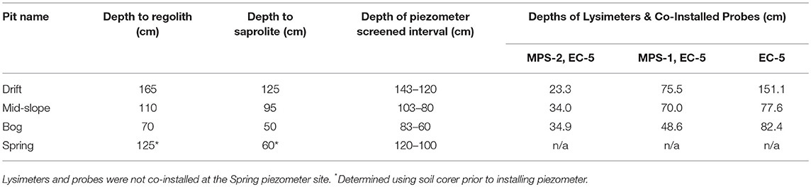
Table 1. Depths of soil contacts and instrument installation for each soil pit.

Three Prenart SuperQuartz (Prenart Equipment ApS, Buen, Denmark) tension lysimeters were installed in each pit at three depths: at ~30 cm below the soil surface, at the soil-saprolite boundary, and in saprolite. Decagon EC-5 (METER Environment Group, USA) soil moisture probes were installed at the same depths as the lysimeters, and Decagon MPS-1 and MPS-2 soil matric potential probes were installed alongside the lysimeters at the soil-saprolite boundary and 10 cm below the soil surface, respectively (Table 1). Soil moisture and matric-potential data from the soil sensors were collected at 10-min intervals on Decagon EM-50 dataloggers. Each pit setup also incorporated a stainless-steel drive-point piezometer, which was hand-driven to refusal, placing the screened interval in the saprolite near the top of the consolidated bedrock. The piezometers were intended to capture water flowing along the bedrock surface, which is a flowpath that McNamara et al. (2005) reported in the nearby Dry Creek watershed, and were sampled during each site visit. Additionally, slug tests (Fetter, 2001) were performed at each piezometer to obtain saprolite hydraulic conductivity (K) values, and surface soil K estimates were derived from Murdock et al. (2018).

A rain sampler was installed at the end of winter in 2017, and collected rain from May through September 2017, minimizing isotopic fractionation by using a foam float inside of a Nalgene bottle housed within an insulating cooler. Large particles were excluded from the sample bottle by a plastic screen, but dust was not removed. National Atmospheric Deposition Program (NADP) dust data from the ID11 site (Reynolds Creek) were compared to the RME results to account for the effects of wet and dry deposition.

Sample Collection, Processing, and Analysis

Soil water samples were collected at least monthly from January to October 2017, after allowing a 3-month settling period for lysimeters (as per Lohse et al., 2013). During the melt and recession period from March to September 2017, samples were collected bi-weekly. Lysimeters were sampled by applying 60 kPa of tension by hand pump for a minimum of 3 h. Piezometers were sampled with a MasterFlex peristaltic pump (ColeParmer Inc., Vernon Hills, IL), and groundwater wells with a stainless-steel bailer (WildCo Inc., Yulee, FL) or polypropylene ball valve bailer. Heavy snowfall precluded sample collection at the Bog until May of 2017; the Drift and Conifer sites could be sampled during this period, as the lysimeter lines extended to areas of low snow accumulation. Similar lines set up in the Bog were initially inaccessible because of treefall, but collection resumed as early as possible in May. Wells were also sampled throughout the entire period with a handful of exceptions: the Cabin well was not sampled when the generator running its electric well pump failed, and the West well was buried by snow until March 2017 and blocked in September 2017.

Stream water grab samples were collected at the weir and in the bog area upstream of the soil pit during each sampling effort. One sample was taken from the Springhouse stream in October 2017.

Rain samples were collected directly from the rain sampler, after homogenizing the sample bottle contents. Snow samples were collected from pits dug to the base of the snowpack in the snowdrift near the Drift pit, with density samples taken every 30 cm and depth-integrated samples used for analyses. One sample, from the East drift (Figure 1B, drift No. 1), was collected using a snow survey tube. Snow samples were double-bagged in zip-top bags and stored at 0°C until analysis. Liquid water samples were collected in Nalgene bottles and stored at 4°C until analyzed. All water samples were vacuum filtered through pre-combusted 0.7 μm Whatman glass fiber filters within 72 h of collection or thaw. Samples were split into portions for carbon, ion, and isotope analyses. Carbon samples were not further processed. For ion and isotopic analyses, samples were filtered through 0.45 μm Puradisc syringe filters.

Dissolved/non-purgeable organic carbon (DOC/NPOC, detection limit [LOD] 0.05 mg/L), dissolved inorganic carbon (DIC, LOD 0.05 mg/L, measured as total inorganic carbon), and total nitrogen (TN, LOD 0.01 mg/L) were run in the ISU Center for Ecological Research and Education (CERE) lab on a Shimadzu Corp (Kyoto, Japan) TOC-V CSH equipped with an ASI-V autosampler and TNM-1 chemiluminescence detector for TN. Spectral characteristics (absorbance, LOD 1 ng/L, and fluorescence index (FI), LOD 30 ng/L, though note calculated FI is unitless) of dissolved organic matter (DOM) of a subset of samples were determined using the Aqualog Fluorescence and Absorbance Spectrometer (Horiba, Irvine, CA, USA) at the University of Vermont. Specific ultraviolet-visual light absorbance (SUVA, reported in L mg C⁻¹ m⁻¹) was calculated by dividing light absorbance at 254 nm by the corresponding DOC concentration and by accounting for the conversion factor from cm to m. For fluorescence analyses, samples were diluted. The excitation (EX) wavelength range spanned from 250 to 600 nm (increment 3 nm) and emission (EM) ranged from 212 to 619 nm (increment 3.34 nm). All excitation emission matrices (EEMs) were blank-subtracted (nanopure water, resistivity 18 MΩ cm⁻¹), corrected for inner filter effects, and Raman normalized (Ohno, 2002; Miller and Blair, 2009). From these data, we computed relevant indices, including the Fluorescence Index (FI), calculated as the intensity at Emission 470 nm divided by the intensity at Emission 520 nm for Excitation at 370 nm (Cory and McKnight, 2005). Water samples were also analyzed for anions, cations, isotopes of oxygen and hydrogen, total nitrogen, and carbon species. Anions (F⁻, Cl⁻, NO${}_2^{-}$, NO${}_3^{-}$, SO${}_4^{2-}$, Br⁻; LOD 0.01 mg/L) were measured using a Dionex (Sunnyvale, California, USA) ICS-5000, at dilutions from 0 to 1:20, with final dilutions depending on signal strength in the ISU Lohse laboratory. A suite of stable cations (Li through U, LOD 0.02 μg/L) were measured in the Center for Archaeology, Materials, and Applied Spectroscopy (CAMAS) lab at Idaho State University on a Thermo X-II series Inductively Coupled Plasma Mass Spectrometer (ICP-MS) equipped with a Cetac 240-position liquid autosampler (ThermoFisher Scientific); dilution was 1:10 sample:deionized water.

To better define subsurface flowpaths, we used water isotopes to trace the movement of water from soil to the saprolite and bedrock. Water isotopes (deuterium and oxygen-18) are commonly used in hydrology as indicators of evapoconcentration (Kendall and Coplen, 2001). Lighter isotopes evaporate more readily, and so water that has been subject to evaporation will show a larger proportion of the heavier isotopes. Transpiration does not have this effect (Hsieh et al., 1998). A subset of stream samples, and end-members from both May and July 2017 were selected for water isotope analysis. A Delta V Advantage mass spectrometer with a ConFlo IV system (Thermo Fisher Scientific, LOD 4,000–10,000 mV) at the CAMAS lab was used to measure deuterium and δ¹⁸O for water samples. All isotope values are reported as per mille (‰) of δD (permissible error 2.00‰) and δ¹⁸O (permissible error 0.20‰) relative to Vienna Mean Standard Ocean Water (VSMOW). δD vs. δ¹⁸O plots of precipitation (rain and snow) samples were regressed to determine the local meteoric water line (LMWL) (Dansgaard, 1964).

Principal Component and End-Member Mixing Analysis

Principal Component Analysis (PCA) is a multivariate factor analysis technique used to determine the primary entities in a mixture (Davis, 1973). In hydrology, it is used to find the lowest possible n-dimensional space in which all observations (e.g., ionic concentrations) will fit within the bounds of a specified accuracy (Christophersen and Hooper, 1992). PCA can be used to identify the expected number of components for an end-member mixing model as described below, and assist in selecting solutes that best identify possible end-members.

End-member mixing analysis (EMMA) is a method to determine which non-stream waters of a catchment are contributing to stream flow (Hooper et al., 1990). Originally focused on soil water contributions, it has expanded to include all possible sources and can also be used to determine if an end-member that supplies water to the stream was missed in sampling. The key assumption in EMMA is that stream water is derived from some combination of source waters, or end-members, whose chemical compositions are unvarying in time and space (Hooper et al., 1990). After PCA is used to determine how many and which solutes are used for EMMA, the concentrations of those solutes in the suspected end-members are used to construct a bounding polygon in n-dimensional space, where the number of vertices (representing each end-member) is equal to the number of solutes plus one (Barthold et al., 2011). EMMA must be adjusted when stream water chemistry points fall outside the bounds of the shape defined by end-member concentrations, typically by adopting different tracers or by projecting the points to the closest (n-1)-dimensional space (Hooper, 2001), which we adopted for the handful of points that fell outside the best-fit end-member space identified by PCA (Christophersen and Hooper, 1992; Liu et al., 2004).

PCA and EMMA were performed using the “stats” package in the R statistical software (Liu et al., 2004; Martins, 2013). Isotopes, carbon, and nitrogen were not used for these analyses due to sampling limitations or non-conservative behavior. Analytes for which fewer than 50% of samples showed measurable concentrations were also excluded. For samples below the detection limit among the remaining analytes, a value of half the detection limit was assumed (after Farnham et al., 2002). Wilcoxon tests were used to determine which potential end-members could be grouped, and stream samples taken at the upstream bog were excluded on this basis. EMMA results are presented here in scaled and centered solute concentrations, rather than U-space, for ease of visualization and interpretation; U-space models gave nearly identical results.

We performed hydrograph separation based on the concentrations of tracers in source and streamwater at each date, and calculated the percent of streamflow for which each end-member was responsible. The fractional contributions of each end-member were then used to calculate a modeled carbon concentration for that stream sample based on end-member DOC concentrations. The modeled DOC was compared to the measured value at each date, using the fractional contribution of each end-member and the carbon concentrations in the end-members on that date, to create a predicted carbon concentration for streamwater and assess the importance of source mixing vs. riparian and in-stream processing of carbon.

Results

Streamflow, Groundwater, and Soil Moisture Responses to Snowmelt

Precipitation events in RME occurred primarily in the fall, winter, and early spring (Figure 2A), consistent with prior observations of strong seasonality of discharge (Figure 2E). During the 2017 water year (WY2017, October 1, 2016-September 30, 2017), snow began accumulating in December 2016 and was entirely melted by mid-June 2017 (Figure 2A).

FIGURE 2

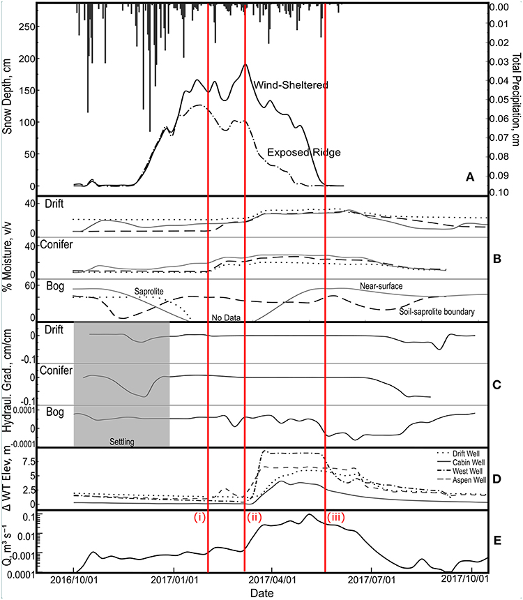
Figure 2. RME inputs, outputs, and changes in storage during water year 2017. (A) Hyetograph on inverse right vertical axis and snow depth on left vertical axis at two sites, the exposed ridge (dashed line) meteorological station (176) and the wind-sheltered snow pillow site (solid line, station “rmsp”). Data from USDA ARS Northwest Watershed Research Center (2017a); USDA ARS Northwest Watershed Research Center. (2017b). (B) Volumetric soil moisture in soil pits—solid lines represent the near-surface measurement, dashed lines represent the soil/saprolite interface, and dotted lines represent the saprolite at all three sites (see Table 1 for installation depths). (C) Hydraulic gradient in soil pits between the 30-cm and soil-saprolite boundary matric potential sensors where common negative gradients indicate downward flow; data from a settling period after installation is grayed out. Note that the scale of the Bog pit differs from the others. (D) Water table elevation relative to lowest recorded level in each of four monitoring wells in RME. (E) Discharge at the catchment-defining weir. Vertical red lines highlight (i) the early March melt event and (ii) peak snow accumulation and increases in soil moisture and water table elevation associated with the onset of melt, and (iii) the end of snowmelt, with succeeding drops in soil moisture and water tables. Spline fits to all data are shown with λ = 0.05, except for wells and discharge panels in which λ = 0.00001; note that the y-axis of the discharge plot is logarithmic.

Soil moisture increased briefly with the onset of snowmelt, and decreased quickly following melt-out, except in the bog (Figure 2B). This pattern is pronounced in the Drift pit, and attenuated in the Conifer pit. In both of these pits, soil moisture remained higher at depth than near the surface throughout WY2017. Extraction of soil water at 60 kPa from the Conifer pit was impossible by June 6th, 2017; the saprolite lysimeter at the Drift site was only able to collect very small (<20 mL) samples after June 6th, and all other lysimeters at these sites remained dry throughout the rest of the summer.

In contrast, the Bog pit was wet throughout the water year. Soil moisture dropped from ~60% to ~45% (volume per volume) in the surface layer between July and October 2017 but remained around 40% at the soil-saprolite interface. We cannot rule out the possibility that the excursion toward zero soil moisture at the soil/saprolite interface (dashed line in Figure 2B) in late winter 2016 may be an artifact because it coincides with the failure of other probes. The soil moisture sensor in the Bog saprolite (dotted line) failed in mid-January 2017, but data from the previous year, which included an extremely dry summer shows little to no change in saprolite water content in the Bog (data not shown). The surface soil moisture sensor in the Bog also failed in mid-January, but resumed data collection in April. This may be due to the aforementioned burial and settling affecting the connection of the probe to the logger, and the changes in soil moisture immediately before and after this failure may also be artifacts. The Conifer and Drift pits both showed a small negative, downward hydraulic gradient for most of the melt period, becoming more negative through the summer (Figure 2C). The hydraulic gradient in the Bog pit varied over a much smaller range than in the other pits, and soil was saturated for most of the year. Piezometers in the Bog and Spring also remained saturated throughout the year. No water was detected in the Drift or Conifer piezometers, and the mud present at the bottom of each piezometer dried out by July 2017.

Wells in RME usually respond to snowmelt nearly as rapidly as soil moisture (Figure 2D). During the snowmelt period of 2017, the soils surrounding the Aspen well were saturated, and formed an ephemeral wetland feeding an intermittent channel into Reynolds Creek. The wetland dried as the summer progressed and the water table dropped, and the initiation of surface flow in the channel moved farther downstream. Piezometers were not instrumented, but during frequent field visits (at least biweekly), water levels in the Bog piezometer were always approximately at the surface of the stream, while those in the Spring piezometer were above the ground surface from March to June 2017. This is consistent with hydraulic conductivity tests performed at these sites: K for surface soils was ~120 cm/day (Murdock et al., 2018), while saprolite K in the piezometers ranged from 2,000 to 11,000 cm/day, with the highest conductivity in the bog. Soils were predominately loams. The saprolite at the Spring piezometer site was so conductive that a slug test could not be successfully performed with our equipment.

Discharge at the weir is near-zero for most of the year, increasing at the start of melt (March 2017) and peaking during the fastest melt period (May 2017). Discharge then drops after all snow has melted, and remains near-zero for the remainder of the year (Figure 2E). Peak discharge occurs in spring or early summer, when snowdrifts in the catchment melt. Flow declines following melt-out until mid to late summer, and then remains fairly consistent—often nearly dry—until the next spring melt, except for brief events associated with late fall snow melt or rain-on-snow events.

Hydrochemistry

Rainfall and Snow Chemistry

Rain and snow represent the most dilute waters in this catchment, as measured across all analytes, with rain being somewhat higher in solutes than snow (Figure 3). Concentrations of cations identified as possible tracers (Rb, Sr, and Ba, see “Sources and Chemistry of Stream Water” section below) in snow were 0.81 ± 1.80, 1.20 ± 0.78, and 33.3 ± 25.0 μg/L (mean ± standard deviation), respectively. In rain, these elements were found at somewhat higher concentrations of 1.93 ± 1.47, 6.12 ± 3.67, and 55.5 ± 43.2 μg/L. DIC and DOC were found in snow at 0.36 ± 0.08 and 1.69 ± 1.82 mg/L, respectively (above the detection limits of 0.05 mg/L), and were also at higher concentrations in rain at 2.74 ± 3.51 and 4.37 ± 2.35 mg/L. SUVA values for DOC in snow and rain were low and very similar to each other [1.16 ± 0.48 and 0.93 (n = 1) L mg C⁻¹ m⁻¹, respectively]. FI in precipitation was generally low, but variable (e.g., FI in snow averaged 2.95 ± 4.38).

FIGURE 3

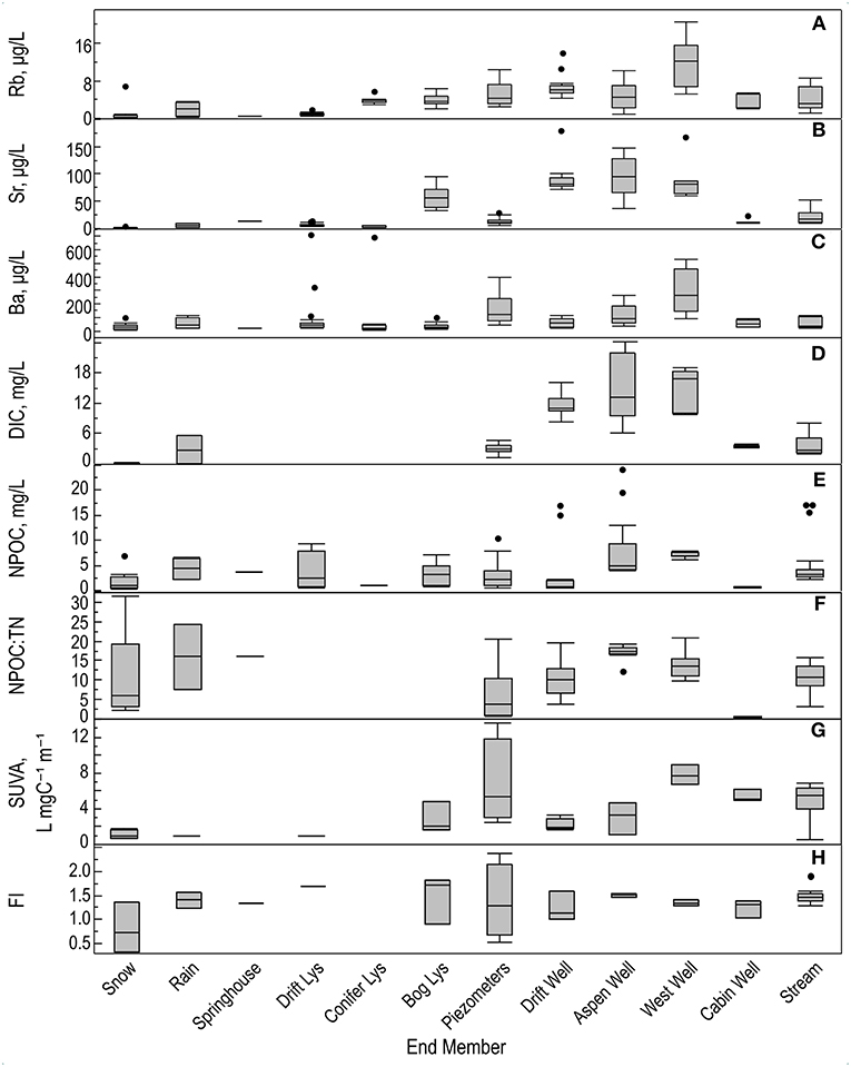
Figure 3. Medians, ranges, and interquartile ranges for (A–C) tracers used in EMMA, (D) DIC, (E) DOC, (F) C:N ratio, (G) SUVA, and (H) FI (see section Results for details) for all potential water sources in RME. Note that only one sample was collected from the Springhouse drift. Missing boxplots for lysimeters are due to insufficient sample to run all analyses.

Spatial Variation in Water Chemistry in Groundwater, Soil Water, and Stream Water

Soil water as measured by tension lysimeters and drive-point piezometers showed strikingly different patterns in solute chemistry compared to groundwater (Figure 3). Mean DIC concentrations were relatively low and invariant in piezometers, 2.90 ± 0.87 and 2.94 ± 0.62 mg/L in the Bog and Spring piezometers, respectively. Insufficient samples were available at the Conifer piezometer to run for DIC, and lysimeter samples were not run for DIC because sampling under higher tension can produce artifacts. Groundwater DIC concentrations were higher than in soil water; the lowest groundwater DIC concentrations were 3.32 ± 0.28 mg/L in the Cabin well. DIC concentrations were higher in the Drift well at 10.80 ± 1.98 mg/L, and the highest average values of 13.44 ± 5.75 and 13.75 ± 3.59 mg/L were found in the Aspen and West wells.

Mean DOC concentrations differed between the Drift, Conifer, and Bog lysimeters, with values of 3.82 ± 3.63, 1.09 (n = 1 because the site was typically dry), and 3.25 ± 2.21 mg/L, respectively. DOC concentrations decreased with depth in the Bog site, from 4.34 ± 1.35 mg/L at 35 cm to 2.43 ± 2.29 mg/L at 82 cm depth. Both Drift and Bog lysimeter concentrations were more variable than the Conifer lysimeter (Figure 3). DOC concentrations in the well samples showed patterns similar to groundwater DIC: they were lowest in the Cabin well and highest in the Aspen and West wells. Average DOC concentrations in the Cabin, Drift, West, and Aspen wells were 0.62 ± 0.13, 3.17 ± 5.69, 7.00 ± 0.56, and 7.92 ± 6.65 mg/L, respectively.

Carbon to nitrogen ratios in the catchment were bounded by the Aspen well (mean ratio [unitless] 17.2 ± 1.9) and Cabin well (0.6 ± 0.1), with the Drift and West wells intermediate between the two. The piezometer C:N ratios were similar to snow and the Cabin well (6.3 ± 6.8). There was insufficient sample from any of the lysimeters to run nitrogen analysis. Piezometer C:N ratios were the most variable, while the Cabin and Aspen well varied the least.

SUVA patterns were similar to those of DOC. Mean SUVA values in soil-water ranged from 0.92 L mgC⁻¹ m⁻¹ in the Drift lysimeter to 2.87 ± 1.70 L mgC⁻¹ m⁻¹ in the Bog lysimeter and were lower than mean SUVA values from the piezometers: 5.37 ± 1.80 L mgC⁻¹ m⁻¹ in the Spring piezometer and 8.062 ± 7.84 L mgC⁻¹ m⁻¹ in the Bog piezometer. The highest groundwater SUVA values were in the West well (7.804.51 ± 1.12 L mgC⁻¹ m⁻¹). SUVA values for the Drift and Aspen wells were similar to one another and the lysimeter values at 2.20 ± 0.69 and 3.00 ± 1.83 L mgC⁻¹ m⁻¹, respectively. The Cabin well had an intermediate mean SUVA value, at 5.41 ± 0.69 L mgC⁻¹ m⁻¹. Soil water FI values varied by location and were possibly lower for the Bog (FI 1.48 ± 0.5, n = 3) than the Drift (FI 1.70, n = 1). FI values varied somewhat between the piezometers, being lower for samples from the Spring piezometer (1.28 ± 0.20), and slightly higher and more variable in the Bog piezometer samples (1.46 ± 1.31). Well sample FI values were generally lower and less variable (1.34 ± 0.06, 1.51 ± 0.04, 1.24 ± 0.19, and 1.33 ± 0.30 for the West, Aspen, Cabin, and Drift wells, respectively).

Rb, Sr, and Ba concentrations were generally lower in lysimeters than wells and piezometers, although the Bog lysimeter showed higher Sr concentrations than its associated piezometer. Rb concentrations were highest in the West well (11.98 ± 5.37 μg/L) and lowest in the Cabin well (3.11 ± 1.48 μg/L), whereas Sr concentrations were highest in the Aspen well (94.1 ± 37.1 μg/L) and lower in the piezometers (Bog, 14.97 ± 6.74; Spring, 11.88 ± 3.16 μg/L) and the Cabin well (13.06 ± 4.33 μg/L). Groundwater Ba concentrations were highest in the West well (278.35 ± 161.14 μg/L) and lowest in the Cabin and Drift wells (56.1 ± 26.0 and 59.0 ± 31.42 μg/L, respectively). Piezometer water had similar mean Ba concentrations to groundwater (211.25 ± 94.23 μg/L for the Bog, 101.28 ± 73.13 μg/L for the Spring), while lysimeter waters were consistently lower (ranging from 107.09 ± 236.28 μg/L for the Conifer lysimeters down to 32.39 ± 18.32 μg/L for the Bog lysimeters). Stream water chemistry overlapped with snow, piezometer, and groundwater samples for all solutes.

Sources and Chemistry of Stream Water

PCA analysis identified strontium (Sr), barium (Ba), and rubidium (Rb) as the best candidates for tracers in EMMA; the principal components these cations represent explain 59% of the variation among samples. These three tracers allowed distinction between four possible end-members (Figures 3A–C). Non-parametric Wilcoxon tests were used to determine which sampled waters represented distinct populations to identify possible unique end-members, and median concentrations of the three tracers were plotted from all identified unique end-members along with individual stream samples (Figure 4). We identified snowmelt, piezometer (saprolite) water, and groundwater from the Drift and Aspen wells as the end-members that best explained observed variations in stream water chemistry (see Figure 1C for well locations). These end-members' concentrations (± their standard deviations) bound 83.3% percent of stream water observations. The small number of stream water samples that fell outside the mixing space had anomalously high Sr, which we posit may have resulted from saprolite water traveling along an alternate unknown flowpath, based on the contemporaneous high Sr concentrations in water sampled from the piezometers.

FIGURE 4

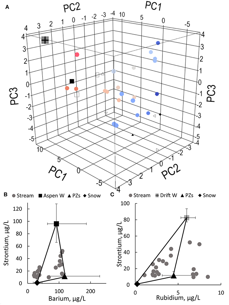
Figure 4. End-member mixing analysis shown in: (A) 3D concentration space, (B) the Ba-Sr plane of concentration space, and (C) the Rb-Sr plane of concentration space. Error bars on end-member median concentrations represent the interquartile range (IQR) of concentration distributions for each end-member, and are not shown if smaller than markers. Stream samples (filled circles) in panel (A) progress in color from blue to red with sample date from March to October 2017. Note that points that fall outside the represented polygon (as in C) are still within the concentration range of each end-member (maximum Rb concentrations for PZs and Drift W, 10.3 and 13.8 ppb, respectively). To solve for the fractional contribution, those points are projected onto the closest plane and values are assumed to be a fractional mix of the end-members comprising that plane (adaptation of the 2D method applied by Liu et al., 2004). See section Results for further discussion of this approach.

Based on the EMMA results, we calculated proportional contributions of each end-member to stream flow at each sampling date (Figures 5A–D). Snowmelt dominates streamflow during the melt period, providing up to 90% of stream water, as indicated by the dilution of some chemical species during this time (Figures 5E–I). As the summer progresses and snow disappears, groundwater and saprolite flow contribute larger proportions of the total discharge, with groundwater providing a cumulative 50% of streamflow on an annual basis. The snowmelt signal declines through the summer but never completely disappears from the hydrograph, suggesting a source of dilute water that contributes to streamflow throughout the year. We note that large variability, especially in Rb and Sr in the piezometer concentrations across sites and during snowmelt, increases uncertainty in estimates of end-member proportions.

FIGURE 5

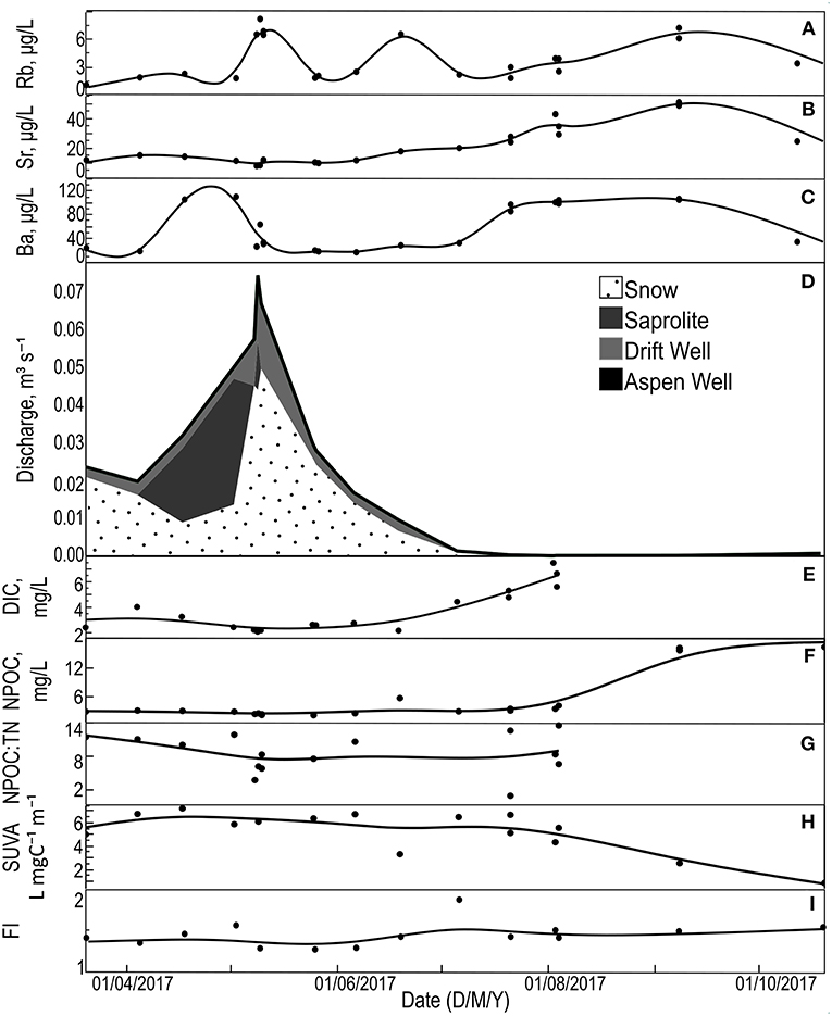
Figure 5. Time series of tracers in streamwater samples (A–C) with spline fits (λ = 0.0002). Contributions of each end-member to streamflow from March to October 2017 (D) calculated using EMMA with the above tracers. Because sampling frequency increased around peak flow, there are more abrupt changes in proportion estimates at this time. Spline fits to DIC, DOC, C:N ratio, SUVA, and FI values (E–I) in the same streamwater samples (λ = 0.05). Samples could not be run for DIC or TN after August due to equipment failure.

Temporal Patterns of Stream Chemistry

Large temporal fluctuations in Rb, Sr, and Ba were observed in the stream (Figures 5A–C). Ba concentrations increased during the snowmelt period prior to peak melt, while Rb concentrations peaked at peak discharge and again later during the melt period. Stream Sr concentrations increased from ~15 μg/L during snowmelt to a peak concentration of ~55 ug/L during late summer.

In contrast to the cations, streamwater carbon concentrations showed distinct seasonal patterns. Streamwater concentrations of DIC were lowest during peak snowmelt, increasing during the summer months (Figure 5E). In contrast, relatively stable DOC concentrations were observed with snowmelt followed by an increase during the summer months (Figure 5F). DOC concentrations and the C:N ratio (Figure 5G) behaved similarly to DIC, with higher values during lower flows (Figures 5F, 6A). The slope of the log(DOC)-log(discharge) relationship is −0.2 ± 0.03 (R${}_{\text{adj}}^2=$ 0.63), which differs significantly from zero (p < 0.001). SUVA exhibits a weak threshold response to flows with values ~2.5–5 L mgC⁻¹ m⁻¹ higher during snowmelt than summer months (Figure 6B). Stream water FI concentrations were relatively constant (mean 1.45), with more variability during melt-out (Figures 5I, 6C).

FIGURE 6

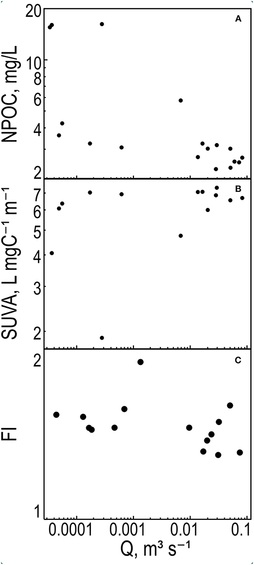
Figure 6. Discharge at the outlet to RME, plotted in log-log space against (A) concentration of dissolved organic carbon, (B) SUVA, and (C) FI. DOC is highly variable at low flows and exhibits slight dilution at high flows, SUVA increases with Q, and FI remains relatively unchanged. Two outliers are not plotted here to facilitate visual comparison among all other samples: one snow sample with a very high FI and one bog piezometer samples with a very high SUVA. Insufficient sample was available to run the latter for nitrate.

The proportional mixing model (Figure 5D) was also used to predict streamwater DOC concentrations (Figure 7), based on the proportional contribution and DOC concentration of each end-member. Predicted DOC concentrations are nearly always lower than observed DOC concentrations, especially during melt (Figure 7). However, the concentration-discharge behavior of DOC is accurately represented: lower DOC concentrations are observed at higher flows (i.e., during snowmelt).

FIGURE 7

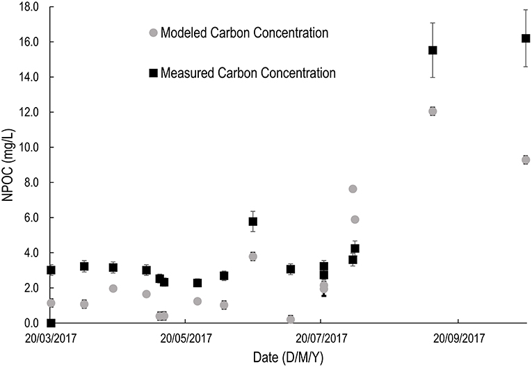
Figure 7. Modeled (gray) and measured (black) DOC concentrations for Reynolds Creek streamwater, based on outcomes of the proportional-mixing model. Measured concentrations displayed with 10% analytical error, which is conservative: actual measurement errors may be less.

Isotopic Signatures and Melt Patterns

Water isotopic results reflect similar mixing and flowpath temporal variation to the cation and nutrient results. The slope of the regression line for the local meteoric water line (LMWL) is 6.9 ± 0.5 (SE), and the intercept is −10.1 ± 7.0 (SE) (R² = 0.98, Figure 8A), within the range of values expected in the continental United States (Kendall and Coplen, 2001). The isotopic regression line for stream water samples in RME has a slope of 6.1 ± 0.5 (SE) (Figure 8B), which does not differ significantly from the slope of the LMWL (p = 0.22). Stream water isotopes become heavier as the summer progresses, indicative of evaporation (Kendall and Coplen, 2001). Water collected from the suction lysimeters in the soil has a slight evaporative signal, with a regression slope of 6.5 ± 0.5 (SE) (Figure 8C) that also does not differ from the slope of the LMWL (p = 0.53) or the stream (p = 0.54). Water drawn from the piezometers in saprolite, on the other hand, is highly evaporated, with a slope of 3.1 ± 0.9 (SE), which is significantly different from the LMWL, streamwater, and soil water (p = 0.0048, 0.001, and 0.0069, respectively; Figure 8D).

FIGURE 8

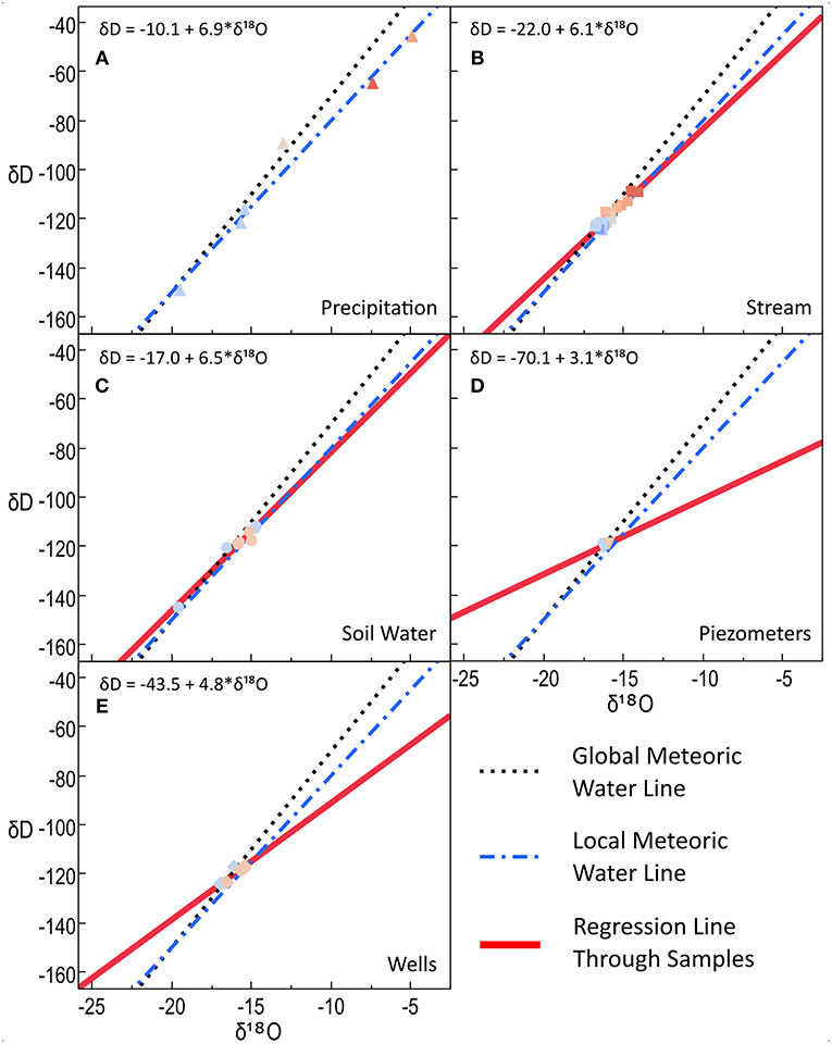
Figure 8. Water isotopes for all waters in RME, by source: (A) precipitation, (B) stream, (C) soil water, (D) saprolite water (piezometers), and (E) groundwater. Points represent samples; point colors progress from blue to red as the sample dates shift from March to July 2017. R${}_{\text{adj}}^2$ for all regression lines varies between 0.7 and 0.97; note that for comparison purposes, axis ranges are held constant across all panels although sample variability is damped in subsurface samples relative to precipitation. The local meteoric water line was determined by a regression of the precipitation samples. Regression lines are extended beyond measured points for visual clarity, and regression formulas are included for each group of samples.

Isotopic signatures of water in the wells at RME are heavier during the early melt stages in May and become lighter and closer to the local meteoric water line (LMWL) as the snowpack disappears in July (Figure 8E). The regression slope of all well samples is 4.8 ± 0.8 (SE), which does not significantly differ from the piezometer (p = 0.18) or lysimeter (p = 0.10) regression slopes, but differs from the LMWL and stream water slopes (p = 0.047, 0.037, respectively).

Geophysics: Electrical Resistivity and Seismic Velocity Data

Seismic velocities on Line 4 range from ~300 m/s at the surface to >4,000 m/s at depths of 40–70 m (Figure 9A). In the volcanic rocks that comprise the watershed here, velocity is primarily controlled by porosity, with low velocity corresponding to high porosity and vice-versa. The seismic results thus indicate a downward decrease in porosity in the upper few tens of meters of the subsurface. In this environment, we expect that porosity in the shallow subsurface is primarily controlled by degree of chemical weathering, the opening of fractures, and pre-existing porosity due to vesicles and flow boundaries in the volcanic rock. The electrical resistivity inversion on the northern half of Line 4 shows a shallow, high-resistivity (1,000–10,000 ohm-m) layer of variable thickness over a north-dipping layer with lower resistivity (5–25 ohm-m). The low-resistivity layer rises toward the surface at the stream—a pattern seen on several other lines in this watershed. The southern part of Line 4 shows more complexity, with a low-resistivity body approaching the surface. Low resistivity can be caused by either clay minerals or water saturation, but the correlation of the low-resistivity layer to an observed surface bog and stream strongly suggests that water saturation controls resistivities here.

FIGURE 9

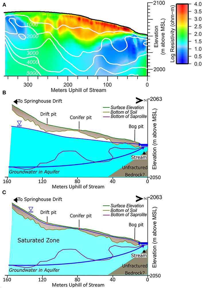
Figure 9. Geophysics results and conceptual models of RME. X-axis is distance from the main stem of Reynolds Creek; the Bog pit is located at a secondary channel. (A) Color scale shows log₁₀ electrical resistivity according to color bar at left. White lines show seismic velocity contours from seismic inversion (italicized numbers in m/s). (B,C) Water table elevation in late summer compared to during snowmelt. Summer water tables (B) are lower, leaving soil water stranded in the unsaturated zone and unable to reach the stream. With the onset of melt, the water table rises (C) and soil water is flushed to the stream. Groundwater in aquifer may be sourced from an adjacent catchment. Note that conceptual figures represent a transect passing through the soil pits which is slightly offset from the geophysical transect, hence the difference in slope profiles; they also represent a shorter horizontal distance from the stream.

Taken together, the seismic velocity and electrical resistivity results allow an interpretation of subsurface architecture, including a hard-rock aquifer at depth. Previous seismic investigations in crystalline rock have interpreted the transition from saprolite to fractured/weathered bedrock to occur at velocities around 1,200–2,000 m/s (e.g., Olona et al., 2010; Befus et al., 2011; Holbrook et al., 2014; Flinchum et al., 2018). Since we lack drilling data connecting porosity to composition and weathering at our site, we approximate the saprolite/fractured bedrock transition at around 1,500 m/s. The velocity of intact, unweathered latite or basalt (McIntyre, 1972) at these depths is expected to be around 5,000 m/s, depending on initial porosity (e.g., Christensen and Salisbury, 1973). Thus, the seismic results suggest a layer of saprolite that is 10–30 m thick, overlying a layer of fractured and weathered bedrock that is 25–50 m thick. While clay minerals are one possible explanation for low resistivities, we would expect clay content to be greater in low-velocity, weathered saprolite, but on our transect the low-velocity layer has the highest resistivities, arguing against clay content as the primary signal. Therefore, given the absence of mapped geological boundaries here, the resistivity data likely indicate the presence of water in the subsurface, with lower resistivity corresponding to higher water content. Moreover, the deep, low-resistivity layer has an orientation that matches velocities of ~2,000–3,500 m/s, velocities appropriate for fractured bedrock (O'Connell and Budiansky, 1974). We therefore interpret the low-resistivity layer on the northern part of the line as a deep aquifer that connects to the surface at the location of the stream. It is unclear whether the southern low-resistivity zone is also an aquifer, though its orientation is suggestive of a recharge zone; while the low-resistivity zones appear disconnected in this transect, they may be the same aquifer, with areas of connection outside the plane of the resistivity transect. Thus, moving down from the surface, the subsurface architecture consists of soil, relatively unsaturated saprolite (during the summer months), a fractured/weathered bedrock aquifer, and finally intact bedrock.

Discussion

What Paths Does Meltwater From Seasonal Drifts Follow on Its Way to the Stream?

Our results suggest four sources of streamwater: snowmelt, flow through the saprolite, and two groundwater flowpaths. Of these sources, snowmelt and groundwater were expected—snowmelt in springtime is generally the largest hydrologic event in this catchment, and a perennial stream in an area with little summer rainfall can almost be guaranteed to have groundwater contributions. The existence of multiple groundwater sources, and the presence of a saprolite layer acting as an aquifer, were unexpected. We propose that the differences in groundwater chemistry derive from differences in the distances from snowdrifts to the stream. We also suggest that the saprolite flowpath reflects a change in saturated hydraulic conductivity between soil, saprolite, and bedrock, creating a perched aquifer. This change in conductivity also inhibits lateral soil connectivity in this catchment; instead the more hydraulically conductive saprolite acts as a preferential flowpath precluding the activation of lateral flowpaths higher up in the soil.

Snowmelt dominates discharge until mid-June, when groundwater and saprolite flow become more important. The continuing snowmelt signal during snow-free periods suggests a dilute source of water in the subsurface. In some systems, soil water would be a candidate source that is more chemically dilute than groundwater, and indeed sampled upland soil waters in RME are chemically very similar to snowmelt (Figure 3). However, previous modeling work in this catchment has suggested that soil saturation is limited to the riparian corridor, where soil waters have a composition more similar to stream water (Grant et al., 2004). Soil saturation data from this study supports limited lateral connectivity of hillslope soils to the stream (Figure 2B). Instead, this snowmelt signal may derive from the Springhouse drift outside the watershed (Figure 1B, drift No. 4); October samples from a stream fed directly from this drift have Ba, Sr, and Rb concentrations very similar to snow. It is possible that soils and rocks along the flowpath from this drift have been so thoroughly leached by several meters of annual precipitation that they now contribute few dissolved ions. That is, the subsurface has been deeply weathered and advective transfer of solutes has already depleted these locations of readily soluble materials (Berner and Berner, 2012).

An alternate explanation for this improbable snowmelt signal lies with the Cabin well. This well is deeper (30 m) than other wells in the catchment and may intersect subsurface flowpaths fed by the Springhouse drift. The Cabin well plots in the center of the stream samples in the EMMA presented in Figure 4. The concentrations of tracers in the Cabin well samples are not variable enough to explain all the variation in stream water chemistry (Figures 3D–H), and the median concentration is not distinct enough to identify the Cabin well as a potential end-member. It is possible that the majority of late-season streamflow is derived from this source, but it is indistinguishable using the methods applied here.

Groundwater in this catchment appears to follow more than one flowpath on its way to the stream. Water from the Aspen well is more chemically variable than water from the Drift well; if we infer flowpaths from surface topography, water in the Drift well would have a short travel time from the East snowdrift directly uphill (Figure 1B, No. 1), while water in the Aspen well could also potentially consist of water from the East drift and another drift located between the two wells (Figure 1B, Nos. 1 and 3, respectively). If the Aspen well were fed by the East drift, that water would have to travel a longer distance, and all else equal, would be expected to have a longer travel time and higher solute concentrations. Multiple water sources could explain the greater variation in hydrochemistry in the Aspen well, as could the surface saturation observed at that site during snowmelt.

Isotopes in groundwater indicate a rapid response to snowmelt, becoming lighter over the melt period (Figure 8E). This could be indicative of the presence of last summer's soil water in the aquifer, or it could reflect isotopic fractionation in the snowpack (Taylor et al., 2001). In the latter case, snowpacks become lighter as melt progresses, and groundwater also becomes lighter from the beginning to the end of melt, as the lighter isotopes eventually enter the aquifer. However, there is evidence in that water entering the aquifer at the beginning of melt is not, in fact, this year's snowmelt. Theoretically, soil water in the capillary fringe should be subject to evapoconcentration (becoming enriched in heavier isotopes), while water located below this fringe in the saprolite and bedrock is not interacting with the atmosphere (Allison, 1998). In RME, the reverse was indicated. Water sampled by lysimeters did not show an evaporative signal, while water from the piezometers was highly evaporated. Based on this, we suggest that soil water which cannot be sampled under 60 kPa tension remains in small pores through the summer, where it is subjected to evaporation, and is then flushed to the saprolite by spring melt. This would explain both the larger evaporative signal and the higher concentrations of Sr, Ba, and Rb in saprolite waters than in sampled soil waters. It would also explain the “lightening” of groundwater during the melt, as the initial pulse of water to the aquifer represents evaporated soil water from the previous year.

The offset of the stream samples from the local meteoric water line suggests that the source of streamwater has already fractionated, which is consistent with saprolite water providing a major portion of streamflow (Sklash and Farvolden, 1979; Kendall and Coplen, 2001). Stream water should be evaporated relative to precipitation (Kendall and Coplen, 2001). In RME, the line of best fit for stream water isotopes had a slope of 5.9, which differs significantly from both the global meteoric water line (slope of 8) and the local meteoric water line defined from precipitation (slope of 7). The difference in slope between the local and global meteoric water lines could be due to evaporation of rainfall in the atmosphere under extremely low-humidity summer conditions (Kendall and Coplen, 2001).

Differences in matric potential between the upper (near surface) and lower (soil/saprolite boundary) matric potential probes in the Drift and Conifer pits indicate an average hydraulic gradient of −6 cm/cm in these soils during the melt period. Combined with the high conductivity of the soils, this suggests a “wetting-up” process in the soil profile, similar to that observed in Dry Creek by McNamara et al. (2005). The high conductivity of the saprolite layer suggests that saturation occurs in the soil profile only once saprolite is saturated, and further supports our hypothesis that the saprolite layer is acting as a perched aquifer during the melt period.

Given the tendency of all the tracers used for our EMMA to concentrate in felsic rocks, it is reasonable to assume the majority of streamwater in RME is interacting with the soil and with the surface bedrock layers (rhyolite and latite, McIntyre, 1972). Barium is the 14th most common element in crustal rocks; it concentrates in felsic magmas and can substitute for Ca in feldspars (Salminen et al., 2005). Strontium and rubidium are both associated with hydrothermal alteration, and can substitute for potassium in feldspars, micas, and clays (Salminen et al., 2005). The presence of hydrothermal alteration in RME is attested to by the occurrence of hydrothermally emplaced mineral deposits in the nearby DeLamar mine (Halsor et al., 1988), and by opal observed during field work in a gully draining into the stream.

The saprolite in this catchment formed from weathered rhyolite and latite (McIntyre, 1972), and is generally high in clay. This would explain similar concentrations of rubidium and barium in saprolite waters and groundwater. Strontium is much lower in saprolite water than in groundwater; this may be related to a reduced tendency for Sr release from feldspars in colder, acidic soils compared to Rb and Ba (Salminen et al., 2005).

The presence of barium in snow suggests there is some atmospheric deposition of this element in RME, but we lack data to test this theory. Barium is not reported at the nearby National Atmospheric Deposition Program (NADP) National Trends Network site ID11. Snow is almost entirely lacking in strontium or rubidium, indicating little interaction with the igneous bedrock of the catchment. Snow is only slightly more dilute than soil water samples from the Drift and Conifer pits, suggesting that soil water moves quickly through the soil to the saprolite during the wetter portions of the year (Grant et al., 2004). This is consistent with both the “flushing” and “fill and spill” hypotheses (Boyer et al., 1997; Tromp-Van Meerveld and McDonnell, 2006).

Stream samples from May 8th to 11th and June 19th are anomalously high in strontium in comparison to all other dates. However, they fall within the range of Sr in saprolite water; Sr concentrations in piezometer samples on those same dates are also above the median value. There is no clear correlation of these excursions to melt or rainfall events.

A Conceptual Model of Subsurface Flow

From our geophysics data (Figure 9A), we determined three hypothetical subsurface flowpaths (shallow soil, saprolite/bedrock interface, and bedrock aquifer, Figures 9B,C). Our hydrochemistry suggests that of these three possible flowpaths, only the saprolite/bedrock interface flow and flow through the aquifer contribute significantly to streamflow. Overland flow is not represented in this figure; however, we observed expansion of the ephemeral channel network during snowmelt, suggesting that much of the meltwater enters channels close to the snowdrift it derives from, and has little interaction with the soil. When the catchment is dry (late summer through winter), the water table is below the soil profile, and soil water on the hillslope is disconnected from the stream (Figure 9B). During the melt period, the water table rises, wetting the soil, as soil water from the previous summer is flushed into the deeper saturated zone, whence it flows to the stream and snowmelt (Figure 9C). There is sufficient ambiguity in the ERT data that this aquifer may be intersected by all or none of the 15 m deep wells or the 30 m deep Cabin well. This data does not allow us to definitively conclude that the Cabin well draws on a separate aquifer from the other wells in the watershed.

Is Soil Water a Major Component of the Hydrograph, or Is Carbon Transported Along Another Subsurface Flowpath?

Although we expected to see SOC become DOC through lateral connectivity of soils and streams, consistent with the flushing hypothesis, we found that when the saprolite becomes a preferential flow path, soil water does not directly contribute to streamflow. Yet soil is the major reservoir and source of DOC—thus, DOC must be carried to the stream by saprolite water or groundwater. DOC concentrations are higher in the Aspen and Drift wells than in the stream, and very similar in the Bog piezometer; only the Spring piezometer has much lower DOC concentrations than the stream (Figure 3B). Saprolite water DOC quality was the most similar to stream water of the potential sources, suggesting that saprolite water is the major source of DOC to Reynolds Creek (Figures 3E–H). Thus, we conclude that while SOC is the primary carbon source for stream DOC in this system, the flowpaths are not controlled by lateral soil connectivity to the riparian zone, but rather by infiltration to the saprolite layer underlying the soil. This work contrasts with the flushing hypothesis, or settings in which DOC concentrations correlate with riparian groundwater depths (e.g., Inamdar et al., 2008). Instead we observe processes analogous to those found by Gannon et al. (2015) and Zimmer and McGlynn (2018), who both emphasize the importance of complex subsurface connections. The detailed mechanisms differ —Gannon et al. (2015) emphasize distal-to-stream connections driven by shallow soils around bedrock and Zimmer and McGlynn (2018) highlight the role of frequent storms driving shallow subsurface connections—whereas here we emphasize soil-saprolite connections driven by drift-melt pulses. These findings, in addition to our results, demonstrate that, although hydrological controls are critical for estimates of aquatic carbon fluxes (Raymond and Saiers, 2010; Leach et al., 2016; Webb et al., 2018), it is important to understand the spatial and temporal constraints on hydrologic processes that drive streamflow. Our observations also highlight the risk of using DOC itself as a tracer: even if the source of carbon for a given catchment is correctly identified, there is a risk that flowpaths will be oversimplified if all SOC is assumed to become DOC by lateral flow of water through soils to the stream.

What Are the Patterns of Dissolved Organic Carbon Concentrations in Stream and Source Waters?

In contrast to our expectation that DOC would increase with increasing discharge (Sanderman et al., 2009), a dilution pattern was observed where increasing discharge led to lower DOC concentrations. Discharge in RME peaks with peak snowmelt, then declines until mid to late summer. DOC concentrations, in contrast, are highest during late summer and lowest during the melt period. This is inconsistent with the flushing hypothesis, where DOC-rich riparian zones become saturated and flush DOC into streams during snowmelt (Boyer et al., 1997; Sanderman et al., 2009). Rather DOC appears to concentrate in soil water during dry periods and be flushed vertically by piston-flow mechanism to the saprolite/bedrock interface during snowmelt. From there it moves laterally to the stream, which accounts for the observed dilution pattern, as surface snowmelt is contributing significantly to streamflow during this period.

Weak DOC dilution at high flows is also inconsistent with emergent chemostatic behavior for DOC, and may be explained by the factors invoked in Creed et al. (2015)—at the event scale, they invoke stability in flowpaths to explain chemostasis; we surmise flowpaths in RME are not stable at the event scale, and so create chemodynamic conditions. We suggest that saprolite/bedrock interface flow is temporally variable (consistent with its variable contribution to streamflow shown in Figure 5D), and soil water flushed to this interface during melt mixes non-conservatively with other soil waters.

Higher discharges are associated with lower DOC but higher SUVA, indicating that snowmelt carries aromatic, possibly “fresher” DOC into the stream. During low discharge summer times, DOC concentrations are high and SUVA values are low, which could indicate that autotrophic processes (algae in the channel) over the summer produce DOC of low aromaticity. However neither DOC dynamics during winter low-flows, nor the consistently low, terrestrial FI values (McKnight et al., 2001) can be explained by this process. Another possibility is that bog and near-bog saturated soils serve as the major source of DOC in late summer. A similar pattern was found by Sanderman et al. (2009) and is in agreement with the low FI values but does not explain the low summer SUVA values. Lastly, delivery of highly decomposed organic carbon from deep soil horizons could drive stream water DOC over the summer (Neff et al., 2006). DOC delivered through deep flow paths should have low SUVA values because aromatic moieties are removed by interaction with mineral surfaces (Meier et al., 1999; Chorover and Amistadi, 2001). Because all streamwater has to transect the hyporheic and riparian zone (Bishop et al., 2004; Winterdahl et al., 2011), the signal would still be terrestrial and exhibit low FI values (Perdrial et al., 2014). Given the high concentrations of carbon in saprolite and groundwater (Figure 3), it seems likely that the majority of DOC in RME is derived from decomposed soil organic matter of terrestrial origin.

Regardless of the DOC source, we can be confident that there is little to no leaching of SOM from surface soil horizons during the summer months. The lack of precipitation (Figure 2A) and hydrologic connectivity, as shown by extremely low soil moisture during the summer months (Figure 2B, and modeled in Grant et al., 2004), mean that there is no mechanism for leaching these horizons until snowmelt.

Integrated Processes Control Carbon Mixing

We integrated multiple lines of evidence, including indices of DOC composition, and performed end-member mixing analysis using relatively conservative tracers to determine the sources of both stream water and DOC in a snowdrift-dominated headwater catchment. Even though soil water is not a major source of streamflow in this catchment, soil organic carbon is the primary carbon source. The explanation for this apparent inconsistency in sources requires a fuller understanding of the hydrological processes at work in the study catchment. These results are comparable with those of Carroll et al. (2018), who similarly found that soil water was not a major direct component of streamflow, but traveled along deeper and variable subsurface pathways.

Because more than 70% of precipitation in RME falls as snow, and is stored in the form of wind-created snowdrifts (Nayak et al., 2010; Reba et al., 2011), these drifts are the ultimate source of stream flow in RME. However, the different paths that water takes to the stream determine stream water chemistry and DOC content. SOC leached to the groundwater throughout the catchment reaches the stream through deep flowpaths as well as flowpaths that follow the soil-bedrock interface. DOC concentration varies little in time, but sources are increasingly affected by microbial processing as the summer progresses.

Streamflow in RME is primarily derived from snowmelt and groundwater, with the groundwater flowpaths being divided between shallow saprolite flow and flow through a deeper fractured-bedrock aquifer. Groundwater is derived from soil water displaced by snowmelt by piston-type flow, where melting snow drives antecedent soil water vertically down through the profile into the saprolite and bedrock aquifers. This is shown by the SOC-like carbon signatures of saprolite and groundwater, and the distinct geochemical fingerprints of water from these aquifers. Stream water in RME shows little evidence of lateral soil connectivity, which we did not expect, given the importance of this mechanism in other studies. Carbon exported by Reynolds Creek flowing from RME is derived ultimately from SOC, but the dilution behavior displayed by DOC with increasing discharge suggests some form of source or rate limitation for carbon export during the melt period.

Comparing modeled DOC concentrations based on EMMA partitioning to measured DOC values for streamwater on the same dates shows a consistent model under-prediction of carbon content (Figure 7). There are several possible explanations for the additional stream DOC not captured by the model. Autochthonous carbon could be a culprit, as could unidentified sources of allochthonous organic matter. In-stream production is highly variable in headwater streams, and often lower than in larger downstream systems (Fisher and Likens, 1973; Creed et al., 2015). Despite the presence of macrophytes in the channel, stream DOC indices from RME were consistent with terrestrial carbon sources. While the majority of the watershed is shrub/grassland or conifer forest, the near-stream riparian zone was dominated by deciduous trees, which could provide a source of terrestrial DOC not transported through the subsurface. However, the carbon-to-nitrogen ratios of the stream and source waters are very similar, suggesting limited addition of carbon to the stream from other sources. Increasing DOC in late summer and autumn is common in headwater streams, linked to higher temperatures increasing turnover and solubility (Dawson et al., 2008; Koenig et al., 2017). In fact, Koenig et al. (2017) inferred that site-to-site seasonal consistency in this pattern was more a function of DOC generation than the bypassing of surface soils because it was unaffected by variations in seasonal snowmelt patterns among sites. Seasonally declining SUVA values at RME indicate that late-summer DOC is more bioavailable than during the rest of the year (Perdue, 1998; Weishaar et al., 2003), and the concurrent slight increase in FI suggests microbial processing may increase in late summer (Kang and Mitchell, 2013; Hosen et al., 2014). FI values are relatively consistent throughout the year suggesting that carbon sources are consistent as well. The exception is a drop in SUVA values and a slight increase in FI values toward the end of the year which is in agreement with increased microbial processing, possibly decomposing leaf litter from riparian vegetation. Another possible source of higher DOC during spring melt is macropore water, or soil water draining under zero tension. Sanderman et al. (2009) showed higher DOC concentrations in macropore compared to matrix (lysimeter) water; these macropore waters overlapped with SOC concentrations. Finally, we cannot rule out an incomplete hydrological model: given that the PCA used to generate the EMMA accounted for only 59% of total variance in streamwater chemistry, it is possible that we overlooked a flowpath with higher DOC.

It is also clear that the use of DOC quality or quantity to determine water end-members in RME would not give the same results as the use of cations in an EMMA, as can be seen from the attempt to create a carbon model using the fractional contributions of end-members to streamflow (Figure 9). The quality of carbon as determined by SUVA and FI indicates a soil carbon source, which in the absence of other data (soil water samples and EMMA) would suggest significant lateral flow through the soils—a flowpath not supported upon further examination. Based on quantity alone, accidental repetition one would expect a larger contribution from the Aspen well would be expected than is indicated by the Ba/Sr/Rb EMMA. Alternatively, the use of SUVA would yield a larger proportion of piezometer water. In the cation-based EMMA, the contributions of both groundwater sources are much smaller than those of snowmelt. This may suggest that SOC is more soluble during the snowmelt period than are than the inorganic tracers, used during the snowmelt period, and so the groundwaters export more DOC than might be expected based on the EMMA alone. It may also indicate unsampled preferential flowpaths high in SOC that route meltwaters to the stream, perhaps along root channels. Snowdrift-dominated, dryland headwater catchments may largely bypass near-surface flowpaths, but still export large DOC fluxes if SOC can be readily flushed during the melt period. While this study leaves significant room for detailed future studies of the impacts of preferential and variable flowpaths, carbon solubility, and in-stream carbon cycling, it does indicate that the use of DOC as a tracer for water sources has problems beyond the non-conservative nature of carbon. Consistent with the work of Carroll et al. (2018), studies using DOC tracers to suggest a high proportion of lateral soil-water flow entering streams may deserve re-evaluation.

Conclusions

In this system, the seasonal flushing of soil water to groundwater by snowmelt creates an isotopically enriched groundwater source with a DOC signature from soil organic matter. This groundwater source sustains stream flow and DOC fluxes during a long dry summer. Variable subsurface flowpaths can increase spatial heterogeneity of water and carbon delivery to streams, but may decrease temporal variability. Repeated high-resolution geophysical surveys could help constrain the flowpaths and processes controlling this delivery. These effects may be especially important in semi-arid or seasonally dry systems, where perennial streams rely on above- and belowground water stores that can dampen the effects of seasonal variations in precipitation. In mountainous settings like RME, the formation of snow drifts can increase spatial variability in water, cation and DOC delivery to groundwater and the stream. Further work to distinguish the possible role of preferential flowpaths from drift accumulation areas, and feedbacks between drifts and vegetation, are needed. For example, in drift areas, greater water availability might lead to increased vegetation growth, and associated organic matter accumulation. Alternately, because of a shortened growing season and overwinter drift movement, drift areas might have less vegetation and lower organic matter accumulation. Snow fence experiments reveal some impacts of snow drifting, but not the potential long-term feedbacks. Furthermore, as the rain-snow transition moves up in elevation—into currently drift-dominated systems like RME—understanding changes to belowground storage becomes essential. Using geophysical imaging to constrain shifts in dominant flowpaths and transmissivity could be a powerful technique to predict impacts on groundwater as climate changes. If groundwater is no longer replenished by a large pulse of water during snowmelt, or if the snowmelt is no longer concentrated in a small area within the watershed, a shift in the timing and magnitude of both water and carbon fluxes would be expected. Given the essential connection between snow-dominated headwater systems and the ability of mountain areas of the world to sustain human populations, understanding the coupling of carbon and water in these catchments should be a high priority for future research.

Data Availability

The datasets generated for this study can be found in the BSU ScholarWorks repository, Boise State University https://doi.org/10.18122/reynoldscreek/10/boisestate.

Author Contributions

AR, SG, KL, and MS conceived the idea. AR completed field work, data analysis, and drafted the manuscript with help from SG, KL, MS, WH, and EM. EM, KL, and JP performed laboratory analysis. MS provided data from the USDA-ARS and assisted in its interpretation. WH performed geophysical surveying and interpretation. All authors assisted in editing the manuscript.

Funding

This study was conducted in collaboration and cooperation with the USDA Agriculture Research Service, Northwest Watershed Research Center, Boise, Idaho, and landowners within the Reynolds Creek Critical Zone Observatory (RC CZO). Support for this research was provided by NSF for RC CZO Cooperative agreement NSF EAR-1331872. Additional support was provided by the Idaho State University Department of Geosciences Geslin Award.

Conflict of Interest Statement

The authors declare that the research was conducted in the absence of any commercial or financial relationships that could be construed as a potential conflict of interest.

Acknowledgments

We thank funders and the USDA-Agricultural Research Service, especially Zane Cram and Barry Caldwell; John Dudgeon, Million Hailemichael, and Bruce Finney at the ISU CAMAS lab; and Nicholas Patton, David Huber, Harmandeep Sharma, Kayla Glossner, Ruth MacNeille, Rituraj Yadev, and Erin Miller for field and/or lab assistance.

References

Allison, G. B. (1998). Stable Isotopes in Soil and Water Studies. Colloques et Séminaires - Institut Français de Recherche Scientifique Pour Le Développement En Coopération, 23–38. Available online at: http://cat.inist.fr/?aModele=afficheN&cpsidt=2279868

Barnett, T. P., and Adam, J. C. (2005). Potential impacts of a warming climate on water availability in snow-dominated regions. Nature 438, 303–309. doi: 10.1038/nature04141

PubMed Abstract | CrossRef Full Text | Google Scholar

Barthold, F. K., Tyralla, C., Schneider, K., Vaché, K. B., Frede, H. G., and Breuer, L. (2011). How many tracers do we need for end member mixing analysis (EMMA)? a sensitivity analysis. Water Resour. Res. 47, 1–14. doi: 10.1029/2011WR010604

CrossRef Full Text | Google Scholar

Befus, K. M., Sheehan, A. F., Leopold, M., Anderson, S. P., and Anderson, R. S. (2011). Seismic constraints on critical zone architecture, Boulder Creek watershed, Front Range, Colorado, Vadose Zone J. 10, 915–927. doi: 10.2136/vzj2010.0108

CrossRef Full Text | Google Scholar

Beniston, M. (2003). Climatic change in mountain regions: a review of possible impacts. Clim. Change 59, 5–31. doi: 10.1023/A:1024458411589

CrossRef Full Text | Google Scholar

Berner, E. K., and Berner, R. A. (2012). Global Environment: Water, Air, and Geochemical Cycles. Princeton, NJ; Oxford: Princeton University Press.

Google Scholar

Bishop, K., Seibert, J., Köhler, S., and Laudon, H. (2004). Resolving the double paradox of rapidly mobilized old water highly variable responses in runoff chemistry. Hydrol. Process. 18, 185–189. doi: 10.1002/hyp.5209

CrossRef Full Text | Google Scholar

Boyer, E. W., Hornberger, G. M., Bencala, K. E., and McKnight, D. M. (1997). Response characteristics of DOC flushing in an alpine catchment. Hydrol. Process. 11, 1635–1647. doi: 10.1002/(SICI)1099-1085(19971015)11:12<1635::AID-HYP494>3.0.CO;2-H

CrossRef Full Text | Google Scholar

Carroll, R. W. H, Bearup, L. A., Brown, W., Dong, W, Bill, M, and Williams, K. H. (2018). Factors controlling seasonal groundwater and solute flux from snow-dominated basins. Hydrol. Process. 32, 2187–2022. doi: 10.1002/hyp.13151

CrossRef Full Text | Google Scholar

Chorover, J., and Amistadi, M. K. (2001). Reaction of forest floor organic matter at colloidal goethite, birnessite and smectite surfaces. Geochim. Cosmochim. Acta 65, 95–109. doi: 10.1016/S0016-7037(00)00511-1

CrossRef Full Text | Google Scholar

Christensen, N. I., and Salisbury, M. H. (1973). Velocities, elastic moduli and weathering-age relations for pacific layer 2 basalts. Earth Planet. Sci. Lett. 19, 461–470. doi: 10.1016/0012-821X(73)90190-8

CrossRef Full Text | Google Scholar

Christophersen, N., and Hooper, R. P. (1992). Multivariate analysis of stream water chemical data: the use of principal components analysis for the end-member mixing problem. Water Resour. Res. 28, 99–107. doi: 10.1029/91WR02518

CrossRef Full Text | Google Scholar

Cole, J. J., Prairie, Y. T., Caraco, N. F., McDowell, W. H., Tranvik, L. J., Striegl, R. G., et al. (2007). Plumbing the global carbon cycle: integrating inland waters into the terrestrial carbon budget. Ecosystems 10, 172–185. doi: 10.1007/s10021-006-9013-8

CrossRef Full Text | Google Scholar

Cory, R. M., and McKnight, D. M. (2005). Fluorescence spectroscopy reveals ubiquitous presence of oxidized and reduced quinones in dissolved organic matter. Environ. Sci. Technol. 39, 8142–8149. doi: 10.1021/es0506962

PubMed Abstract | CrossRef Full Text | Google Scholar

Cowardin, L. M., Carter, V., Golet, F. C., and LaRoe, E. T. (1979). Classification of Wetlands and Deepwater Habitats of the United States. US Department of the Interior, US Fish and Wildlife Service.

Cox, P. M., Betts, R. A., Jones, C. D., Spall, S. A., and Totterdell, I. J. (2000). Acceleration of global warming due to carbon-cycle feedbacks in a coupled climate model. Nature 408, 184–187. doi: 10.1038/35041539

PubMed Abstract | CrossRef Full Text | Google Scholar

Creed, I. F., McKnight, D. M., Pellerin, B. A., Green, M. B., Bergamaschi, B. A., Aiken, G. R., et al. (2015). The river as a chemostat: fresh perspectives on dissolved organic matter flowing down the river continuum. Can. J. Fish. Aquat. Sci. 72, 1272–1285. doi: 10.1139/cjfas-2014-0400

CrossRef Full Text | Google Scholar

Crimmins, S. M., Dobrowski, S. Z., Greenberg, J. A., Abatzoglou, J. T., and Mynsberge, A. R. (2011). Changes in climatic water balance drive downhill shifts in plant species' optimum elevations. Science 331, 324–327. doi: 10.1126/science.1199040

PubMed Abstract | CrossRef Full Text | Google Scholar

Dansgaard, W. (1964). Stable isotopes in precipitation. Tellus 16, 436–468. doi: 10.3402/tellusa.v16i4.8993

CrossRef Full Text | Google Scholar

Davis, J. C. (1973). Statistics and Data Analysis in Geology. New York, NY: Wiley.

Google Scholar

Dawson, J. J. C., Soulsby, C., Tetzlaff, D., Hrachowitz, M., Dunn, S. M., and Malcom, I. A. (2008). Influence of hydrology and seasonality on DOC exports from three contrasting upland catchments. Biogeochemistry 90, 93–113. doi: 10.1007/s10533-008-9234-3

CrossRef Full Text | Google Scholar

Dingman, S. L. (2015). Physical Hydrology, 3rd Edn. Long Grove, IL: Waveland Press.

Google Scholar

Doran, J. W. (2002). Soil health and global sustainability: translating science into practice. Agric. Ecosyst. Environ. 88, 119–127. doi: 10.1016/S0167-8809(01)00246-8

CrossRef Full Text | Google Scholar

Ekren, E. B., McIntyre, D. H., Bennet, E. H., and Malde, H. E. (1981). Geologic Map of Owyhee County, Idaho, West of Longitude 116° W [map]. 1:125,000. Miscellaneous Investigations Series, Map I-1256. Denver, CO: US Geological Survey.

Google Scholar

Eswaran, H., Berg, E., Reich, P., Van Den Berg, E., and Reich, P. (1993). Organic carbon in soils of the world. Soil Sci. Soc. Am. J. 57, 192–194. doi: 10.2136/sssaj1993.03615995005700010034x

CrossRef Full Text | Google Scholar

Farnham, I. M., Singh, A. K., Stetzenbach, K. J., and Johannesson, K. H. (2002). Treatment of nondetects in multivariate analysis of groundwater geochemistry data. Chemometrics Intel. Lab. Syst. 60, 265–281. doi: 10.1016/S0169-7439(01)00201-5

CrossRef Full Text | Google Scholar

Fellows, A., Flerchinger, G. N., Seyfried, M. S., Lohse, K.A., and Patton, N. R. (2018). Controls on gross production in an aspen-sagebrush vegetation mosaic. Ecohydrology 12:e2046. doi: 10.1002/eco.2046

CrossRef Full Text | Google Scholar

Fetter, C. W. (2001). Applied Hydrogeology, 4th ed. Upper Saddle River, NJ: Prentice-Hall.

Google Scholar

Fiebig, D. M., Lock, M. A., and Neal, C. (1990). Soil water in the riparian zone as a source of carbon for a headwater stream. J. Hydrology 116, 217–237. doi: 10.1016/0022-1694(90)90124-G

CrossRef Full Text | Google Scholar

Fisher, S. G., and Likens, G. E. (1973). Energy flow in Bear Brook, New Hampshire: an integrative approach to stream ecosystem metabolism. Ecol. Monogr. 43, 421–439. doi: 10.2307/1942301

CrossRef Full Text | Google Scholar

Fleckenstein, J. H., Niswonger, R. G., and Fogg, G. E. (2006). River-aquifer interactions, geologic heterogeneity, and low-flow management. Ground Water 44, 837–852. doi: 10.1111/j.1745-6584.2006.00190.x

PubMed Abstract | CrossRef Full Text | Google Scholar

Flerchinger, G.D., Marks, D., Reba, M.L., Yu, Q., and Seyfried, M. (2010). Surface fluxes and water balance of spatially varying vegetation within a small mountainous headwater catchment. Hydrol. Earth Syst. Sci. 14, 965–978. doi: 10.5194/hess-14-965-2010

CrossRef Full Text | Google Scholar

Flinchum, B. A., Holbrook, W. S., Rempe, D., Moon, S., Riebe, C. S., Carr, B. J., et al. (2018). Critical zone structure under a granite ridge inferred from drilling and three-dimensional seismic refraction data, J. Geophys. Res. Earth Surface 123, 1317–1343. doi: 10.1029/2017JF004280

CrossRef Full Text | Google Scholar

Gannon, J. P., Bailey, S. W., McGuire, K. J., and Shanley, J. B. (2015). Flushing of distal hillslopes as an alternative source of stream dissolved organic carbon in a headwater catchment. Water Resour. Res. 51, 8114–8128. doi: 10.1002/2015WR016927

CrossRef Full Text | Google Scholar

Grant, L. E., Seyfried, M. S., and McNamara, J. P. (2004). Spatial variation and temporal stability of soil water in a snow-dominated, mountain catchment. Hydrol. Process. 18, 3493–3511. doi: 10.1002/hyp.5798

CrossRef Full Text | Google Scholar

Grünewald, T., Schirmer, M., Mott, R., and Lehning, M. (2010). Spatial and temporal variability of snow depth and SWE in a small mountain catchment. Cryosphere Discuss. 4, 1–30. doi: 10.5194/tcd-4-1-2010

CrossRef Full Text | Google Scholar

Halsor, S. P., Bornhorst, T. J., Beebe, M., Richardson, K., and Strowd, W. (1988). Geology of the DeLamar silver mine, Idaho - a volcanic dome complex and genetically associated hydrothermal system. Econ. Geol. 83, 1159–1169. doi: 10.2113/gsecongeo.83.6.1159

CrossRef Full Text | Google Scholar

Holbrook, W. S., Riebe, C. S., Elwaseif, M., Hayes, J. L., Basler-Reeder, K., Harry, D. L., et al. (2014). Geophysical constraints on deep weathering and water storage potential in the southern sierra critical zone observatory, Earth Surface Process. Landforms 39, 366–380. doi: 10.1002/esp.3502

CrossRef Full Text | Google Scholar

Hood, E., Gooseff, M. N., and Johnson, S. L. (2006). Changes in the character of stream water dissolved organic carbon during flushing in three small watersheds, Oregon. J. Geophys. Res. Biogeosci. 111, 1–8. doi: 10.1029/2005JG000082

CrossRef Full Text | Google Scholar

Hooper, R. P. (2001). Applying the scientific method to small catchment studies: a review of the Panola Mountain experience. Hydrol. Process. 15, 2039–2050. doi: 10.1002/hyp.255

CrossRef Full Text | Google Scholar

Hooper, R. P., Christophersen, N., Peters, N. E., Neal, C., Hooper, R. P., Vogt, R. D., et al. (1990). Modelling streamwater chemistry as a mixture of soilwater end-members—An application to the Panola Mountain catchment, Georgia, U.S.A. J. Hydrol. 116, 321–343. doi: 10.1016/0022-1694(90)90131-G

CrossRef Full Text | Google Scholar

Hornberger, G. M., Bencala, K. E., and McKnight, D. M. (1994). Hydrological controls on dissolved organic carbon during snowmelt in the snake river near Montezuma, Colorado. Biogeochemistry 25, 147–165. doi: 10.1007/BF00024390

CrossRef Full Text | Google Scholar

Hosen, J. D., McDonough, O. T., Febria, C. M., and Palmer, M. A. (2014). Dissolved organic matter quality and bioavailability changes across an urbanization gradient in headwater streams. Environ. Sci. Technol. 48, 7817–7824. doi: 10.1021/es501422z

PubMed Abstract | CrossRef Full Text | Google Scholar

Hsieh, J. C. C., Chadwick, O. A., Kelly, E. F., and Savin, S. M. (1998). Oxygen isotopic composition of soil water: quantifying evaporation and transpiration. Geoderma 82, 269–293. doi: 10.1016/S0016-7061(97)00105-5

CrossRef Full Text | Google Scholar

Inamdar, S., Rupp, J., and Mitchell, M. (2008). Differences in dissolved organic carbon and nitrogen responses to storm-event and ground-water conditions in a forested, glaciated watershed in western New York. J. Am. Water Res. Assoc. 44, 1458–1473. doi: 10.1111/j.1752-1688.2008.00251.x

CrossRef Full Text | Google Scholar

Intergovernmental Panel on Climate Change. (2014). Climate Change 2013 - The Physical Science Basis. Intergovernmental Panel on Climate Change. Cambridge: Cambridge University Press.

Jones, C. D., McConnell, C., Coleman, K., Cox, P. M., Falloon, P., Jenkinson, D., et al. (2005). Global climate change and soil carbon stocks; predictions from two contrasting models for the turnover of organic carbon in soil. Global Change Biol. 11, 154–166. doi: 10.1111/j.1365-2486.2004.00885.x

CrossRef Full Text | Google Scholar

Kang, P. G., and Mitchell, M. J. (2013). Bioavailability and size-fraction of dissolved organic carbon, nitrogen, and sulfur at the Arbutus Lake watershed, Adirondack Mountains, NY. Biogeochemistry 115, 213–234. doi: 10.1007/s10533-013-9829-1

CrossRef Full Text | Google Scholar

Kendall, C., and Coplen, T. B. (2001). Distribution of oxygen-18 and deuteriun in river waters across the United States. Hydrol. Process. 15, 1363–1393. doi: 10.1002/hyp.217

CrossRef Full Text | Google Scholar

Klos, P. Z., Link, T. E., and Abatzoglou, J. T. (2014). Extent of the rain-snow transition zone in the western U.S. under historic and projected climate. Geophys. Res. Lett. 41, 4560–4568. doi: 10.1002/2014GL060500

CrossRef Full Text | Google Scholar

Koenig, L. E., Shattuck, M. D., Snyder, L. E., Potter, J. D., and McDowell, W. H. (2017). Deconstructing the effects of flow on doc, nitrate, and major ion interactions using a high-frequency aquatic sensor network. Water Resour. Res. 53, 10655–10673. doi: 10.1002/2017WR020739

CrossRef Full Text | Google Scholar

Lapworth, D. J., Gooddy, D., Butcher, A., and Morris, B. (2008). Tracing groundwater flow and sources of organic carbon in sandstone aquifers using fluorescence properties of dissolved organic matter (DOM). Appl. Geochem. 23, 3384–3390. doi: 10.1016/j.apgeochem.2008.07.011

CrossRef Full Text | Google Scholar

Leach, J. A., Larsson, A., Wallin, M. B., Nilsson, M. B., and Laudon, H. (2016). Twelve year interannual and seasonal variability of stream carbon export from a boreal peatland catchment. J. Geophys. Res. Biogeosci. 121, 1851–1866. doi: 10.1002/2016JG003357

CrossRef Full Text | Google Scholar

Li, L., Bao, C., Sullivan, P. L., Brantley, S. L., Shi, Y., and Duffy, C. J. (2017). Understanding watershed hydrogeochemistry: 2. Synchronized hydrological and geochemical processes drive stream chemostatic behavior. Water Resour. Res. 53, 2346–2367. doi: 10.1002/2016WR018935

CrossRef Full Text | Google Scholar

Lindsay, R. (2018) “Peatland classification,” in The Wetland Book, eds C. Max Finlayson, G. R. Guntenspergen, B. A. Middleton, R. McInnes, R. C. Gardner, M. Everard, N. C. Davidson, A. van Dam, K. Irvine, and H. MacKay (Dordrecht: Springer).

Google Scholar

Liu, F., Williams, M. W., and Caine, N. (2004). Source waters and flow paths in an alpine catchment, Colorado Front Range, United States. Water Resour. Res. 40, 1–16. doi: 10.1029/2004WR003076

CrossRef Full Text | Google Scholar

Lohse, K. A., Brooks, P. D., McIntosh, J. C., Meixner, T., and Huxman, T. E. (2009). Interactions between biogeochemistry and hydrologic systems. Ann. Rev. Environ. Resour. 34, 65–96. doi: 10.1146/annurev.environ.33.031207.111141

CrossRef Full Text | Google Scholar

Lohse, K. A., Sanderman, J., and Amundson, R. (2013). Identifying sources and processes influencing nitrogen export to a small stream using dual isotopes of nitrate. Water Resour. Res. 49, 5715–5731. doi: 10.1002/wrcr.20439

CrossRef Full Text | Google Scholar

Marks, D., Cooley, K.R., Robertson, D.C., and Winstral, A (2001). Long-term snow database, Reynolds Creek Experimental Watershed, Idaho, USA. Water Resour. Res. 37, 2835–2838. doi: 10.1029/2001WR000416

CrossRef Full Text | Google Scholar

Marks, D., Winstral, A., Reba, M., Pomeroy, J., and Kumar, M. (2013). An evaluation of methods for determining during-storm precipitation phase and the rain/snow transition elevation at the surface in a mountain basin. Adv. Water Resour. 55, 98–110. doi: 10.1016/j.advwatres.2012.11.012

CrossRef Full Text | Google Scholar

Martins, T. G. (2013). Computing and Visualizing PCA in R. Available online at: http://tgmstat.wordpress.com/2013/11/28/computing-and-visualizing-pca-in-r/

McIntyre, D. H. (1972). Cenozoic geology of the Reynolds Creek Experimental Watershed, Owyhee County, Idaho. Pamphlet 151. Moscow, ID.

McKnight, D. M., Boyer, E. W., Westerhoff, P. K., Doran, P. T., Kulbe, T., and Andersen, D. T. (2001). Spectrofluorometric characterization of dissolved organic matter for indication of precursor organic material and aromaticity. Limnol. Oceanogr. 46, 38–48. doi: 10.4319/lo.2001.46.1.0038

CrossRef Full Text | Google Scholar

McNamara, J. P., Chandler, D. G., Seyfried, M. S., and Achet, S. (2005). Soil moisture states, lateral flow, and streamflow generation in a semi-arid, snowmelt-driven catchment. Hydrol. Process. 19, 4023–4038. doi: 10.1002/hyp.5869

CrossRef Full Text | Google Scholar

Meier, M., Namjesnik-Dejanovic, K., Maurice, P. A., Chin, Y-P., and Aiken, G. R. (1999). Fractionation of aquatic natural organic matter upon sorption to goethite and kaolinite. Chem. Geol. 157, 275–284. doi: 10.1016/S0009-2541(99)00006-6

CrossRef Full Text | Google Scholar

Miller, R. E., and Blair, P. D. (2009). Input-Output Analysis: Foundations and Extensions, 2nd Edn. Cambridge: Press, Cambridge University.

Google Scholar

Murdock, M. D., Huber, D. P., Seyfried, M. S., Patton, N. R., and Lohse, K. A. (2018). Dataset for Soil Hydraulic Parameter Estimates Along an Elevation Gradient in Dryland Soils [Data set]. BSU ScholarWorks, Boise State University

Nayak, A., Marks, D., Chandler, D. G., and Seyfried, M. S. (2010). Long-term snow, climate, and streamflow trends at the Reynolds Creek Experimental Watershed, Owyhee Mountains, Idaho, United States. Water Resour. Res. 46:W06519. doi: 10.1029/2008WR007525

CrossRef Full Text | Google Scholar

Neff, J. C., Finlay, J. C., Zimov, S. A., Davydov, S. P., Carrasco, J. J., Schuur, E. A. G., et al. (2006). Seasonal changes in the age and structure of dissolved organic carbon in Siberian rivers and streams. Geophys. Res. Lett. 33:L23401. doi: 10.1029/2006GL028222

CrossRef Full Text | Google Scholar

O'Connell, R. J., and Budiansky, B. (1974). Seismic velocities in dry and saturated cracked solids. J. Geophys. Res. 79, 5412–5426.

Google Scholar

Ohno, T. (2002). Fluorescence inner-filtering correction for determining the humification index of dissolved organic matter. Environ. Sci. Technol. 36, 742–746. doi: 10.1021/es0155276

PubMed Abstract | CrossRef Full Text | Google Scholar

Olona, J., J. A. Pulgar, G. Fernandez-Viejo, C. Lopez-Fernandez, and J. M., Gonzalez-Cortina (2010). Weathering variations in a granitic massif and related geotechnical properties through seismic and electrical resistivity methods. Near Surface Geophys. 8, 585–599. doi: 10.3997/1873-0604.2010043

CrossRef Full Text | Google Scholar

Patton, N. R., Lohse, K.A., Godsey, S.E., Crosby, B.T., and Seyfried, M.S. (2018). Predicting soil thickness on soil mantled hillslopes. Nat. Commun. 9:3329. doi: 10.1038/s41467-018-05743-y

PubMed Abstract | CrossRef Full Text | Google Scholar

Perdrial, J. N., McIntosh, J. C., Harpold, A., Brooks, P. D., Zapata-Rios, X., Ray, J., et al. (2014). Stream water carbon controls in seasonally snow-covered mountain catchments: impact of inter annual variability of water fluxes, catchment aspect and seasonal processes. Biogeochemistry 118, 273–290. doi: 10.1007/s10533-013-9929-y

CrossRef Full Text | Google Scholar

Perdue, E. M. (1998). “Chemical composition, structure, and metal binding properties,” in Aquatic humic substances, eds D. O. Hessen and L. J. Tranvik (New York, NY: Springer), 41–61.

Google Scholar

Pomeroy, J. W., Gray, D. M., Brown, T., Hedstrom, N., Quinton, W. L., Granger, R. J., et al. (2007). The cold regions hydrological model: a platform for basing process representation and model structure on physical evidence. Hydrol. Process. 21, 2650–2667. doi: 10.1002/hyp.6787

CrossRef Full Text | Google Scholar

Raymond, P. A., and Saiers, J. E. (2010). Event controlled DOC export from forested watersheds. Biogeochemistry 100, 197–209. doi: 10.1007/s10533-010-9416-7

CrossRef Full Text | Google Scholar

Reba, M. L., Marks, D., Seyfried, M. S., Winstral, A., Kumar, M., and Flerchinger, G. (2011). A long-term data set for hydrologic modeling in a snow-dominated mountain catchment. Water Resour. Res. 47, 1–7. doi: 10.1029/2010WR010030

CrossRef Full Text | Google Scholar

Salminen, R., Batista, M. J., Bidovec, M. D., Demetriades, A., De Vivo, B., De Vos, W., et al. (2005). FOREGS Geochemical Atlas of Europe, Part 1: Background Information, Methodology and Maps. Available online at: http://weppi.gtk.fi/publ/foregsatlas/

Sanderman, J., Lohse, K. A., Baldock, J. A., and Amundson, R. (2009). Linking soils and streams: sources and chemistry of dissolved organic matter in a small coastal watershed. Water Resour. Res. 45:W03418. doi: 10.1029/2008WR006977

CrossRef Full Text | Google Scholar

Seyfried, M. S., Grant, L. E., Marks, D., Winstral, A., and McNamara, J. P. (2009). Simulated soil water storage effects on streamflow generation in a mountainous snowmelt environment, Idaho, USA. Hydrol. Process. 23, 858–873. doi: 10.1002/hyp.7211

CrossRef Full Text | Google Scholar

Seyfried, M. S., Harris, R., Marks, D., and Jacob, B. (2001). Geographic database, Reynolds Creek Experimental Watershed, Idaho, United States. Water Resour. Res. 37, 2825–2829. doi: 10.1029/2001WR000414

CrossRef Full Text | Google Scholar

Shrestha, R. (2016). 2009 1m Snow Depth for Reynolds Mountain East, Reynolds Creek Experimental Watershed. Boise State University.

Sklash, M. G., and Farvolden, R. N. (1979). The role of groundwater in storm runoff. J. Hydrol. 43, 45–65. doi: 10.1016/0022-1694(79)90164-1

CrossRef Full Text | Google Scholar

Soulsby, C., Tetzlaff, D., Rodgers, P., Dunn, S. M., and Waldron, S. (2006). Runoff processes, stream water residence times and controlling landscape characteristics in a mesoscale catchment: an initial evaluation. J. Hydrol. 325, 197–221. doi: 10.1016/j.jhydrol.2005.10.024

CrossRef Full Text | Google Scholar

St. Clair, J., Moon, S., Holbrook, W. S., Perron, J. T., Riebe, C. S., Martel, S. J., et al. (2015). Geophysical imaging reveals topographic stress control of bedrock weathering. Science 350, 534–538. doi: 10.1126/science.aab2210

PubMed Abstract | CrossRef Full Text | Google Scholar

Stieglitz, M., Shaman, J., McNamara, J. P., Engel, V., Shanley, J. B., and Kling, G. W. (2003). An approach to understanding hydrologic connectivity on the hillslope and the implications for nutrient transport. Global Biogeochem. Cycles 17, 1–15. doi: 10.1029/2003GB002041

CrossRef Full Text | Google Scholar

Stielstra, C. M., Lohse, K. A., Chorover, J., McIntosh, J. C., Barron-Gafford, G. A., Perdrial, J. N., et al. (2015). Climatic and landscape influences on soil moisture are primary determinants of soil carbon fluxes in seasonally snow-covered forest ecosystems. Biogeochemistry 123, 447–465. doi: 10.1007/s10533-015-0078-3

CrossRef Full Text | Google Scholar

Sturm, M., and Wagner, A. M. (2010). Using repeated patterns in snow distribution modeling: an Arctic example. Water Resour. Res. 46, 1–15. doi: 10.1029/2010WR009434

CrossRef Full Text | Google Scholar

Taylor, S., Feng, X., Kirchner, J. W., Osterhuber, R., Klaue, B., and Renshaw, C. E. (2001). Isotopic evolution of a seasonal snowpack and its melt. Water Resour. Res. 37, 759–769. doi: 10.1029/2000WR900341

CrossRef Full Text | Google Scholar

Tennant, C. J., Harpold, A. A., Lohse, K. A., Godsey, S. E., Crosby, B. T., Larsen, L. G., et al. (2017). Regional sensitivities of seasonal snowpack to elevation, aspect, and vegetation cover in western North America. Water Resour. Res. 53, 6908–6926. doi: 10.1002/2016WR019374

CrossRef Full Text | Google Scholar

Tetzlaff, D., Malcolm, I. A., and Soulsby, C. (2007). Influence of forestry, environmental change and climatic variability on the hydrology, hydrochemistry and residence times of upland catchments. J. Hydrol. 346, 93–111. doi: 10.1016/j.jhydrol.2007.08.016

CrossRef Full Text | Google Scholar

Tromp-Van Meerveld, H. J., and McDonnell, J. J. (2006). Threshold relations in subsurface stormflow: 2. the fill and spill hypothesis. Water Resour. Res. 42, 1–11. doi: 10.1029/2004WR003800

CrossRef Full Text | Google Scholar

USDA ARS Northwest Watershed Research Center. (2017a). [Reynolds Creek 166 hourly streamflow]. Unpublished raw data.

USDA ARS Northwest Watershed Research Center. (2017b). [Reynolds Mountain East Meteorological Data.] Unpublished raw data.

Viviroli, D., Dürr, H. H., Messerli, B., Meybeck, M., and Weingartner, R. (2007). Mountains of the world, water towers for humanity: typology, mapping, and global significance. Water Resour. Res. 43, 1–13. doi: 10.1029/2006WR005653

CrossRef Full Text | Google Scholar

Webb, J. R., Santos, I. R., Maher, D. T., and Finlay, K. (2018). The importance of aquatic carbon fluxes in net ecosystem carbon budgets: a catchment-scale review. Ecosystems 21, 1–20. doi: 10.1007/s10021-018-0284-7

CrossRef Full Text | Google Scholar

Weishaar, J. L., Aiken, G. R., Bergamaschi, B. A., Fram, M. S., Fujii, R., and Mopper, K. (2003). Evaluation of specific ultraviolet absorbance as an indicator of the chemical composition and reactivity of dissolved organic carbon. Environ. Sci. Technol. 37, 4702–4708. doi: 10.1021/es030360x

PubMed Abstract | CrossRef Full Text | Google Scholar

Wickland, K. P., Neff, J. C., and Aiken, G. R. (2007). Dissolved organic carbon in Alaskan boreal forest: sources, chemical characteristics, and biodegradability. Ecosystems 10, 1323–1340. doi: 10.1007/s10021-007-9101-4

CrossRef Full Text | Google Scholar

Williams, M. W., Losleben, M. V., and Hamann, H. B. (2002). Alpine areas in the Colorado Front Range as monitors of climate change and ecosystem response. Geograph. Rev. 92, 180–191. doi: 10.2307/4140969

CrossRef Full Text | Google Scholar

Winstral, A., and Marks, D. (2002). Simulating wind fields and snow redistribution using terrain-based parameters to model snow accumulation and melt over a semi-arid mountain catchment. Hydrol. Process. 16, 3585–3603. doi: 10.1002/hyp.1238

CrossRef Full Text | Google Scholar

Winstral, A., and Marks, D. (2014). Long-term snow distribution observations in a mountain catchment: assessing variability, time stability, and the representativeness of an index site. Water Resour. Res. 50, 293–305. doi: 10.1002/2012WR013038

CrossRef Full Text | Google Scholar

Winterdahl, M., Temnerud, J., Futter, M. N., Löfgren, S., Moldan, F., and Bishop, K. (2011). Riparian zone influence on stream water dissolved organic carbon concentrations at the Swedish integrated monitoring sites. AMBIO. J. Hum. Environ. 40, 920–930. doi: 10.1007/s13280-011-0199-4

PubMed Abstract | CrossRef Full Text | Google Scholar

Zimmer, M. A., and McGlynn, B. L. (2018). Lateral, vertical, and longitudinal source area connectivity drive runoff and carbon export across watershed scales. Water Resour. Res. 54, 1576–1598. doi: 10.1002/2017WR021718

CrossRef Full Text | Google Scholar

Zogg, G. P., Zak, D. R., Ringelberg, D. B., White, D. C., MacDonald, N. W., and Pregitzer, K. S. (1997). Compositional and functional shifts in microbial communities due to soil warming. Soil Sci. Soc. Am. J. 61:475. doi: 10.2136/sssaj1997.03615995006100020015x

CrossRef Full Text | Google Scholar