Metrics and Models for Quantifying Ecological Resilience at Landscape Scales

Introduction

Ecological resilience is a measure of the amount of perturbation required to change an ecosystem from one set of processes and structures to a different set of processes and structures, or the amount of disturbance that a system can withstand before it shifts into a new regime or alternative stable state (Holling, 1973; Curtin and Parker, 2014). In applied ecology, ecological resilience is also used as a measure of the capacity of an ecosystem to regain its fundamental structure, processes and functioning despite stresses, disturbances, or invasive species (e.g., Hirota et al., 2011; Chambers et al., 2014a; Pope et al., 2014; Seidl et al., 2016). Much of the original literature on ecological resilience focused on theory, definitions, and conceptual ideas regarding resilience concepts (e.g., Gunderson, 2000; Folke et al., 2004, 2010; Walker et al., 2004; Gunderson et al., 2010). A major focus early resilience research was the importance of species diversity and species functional attributes related their response to stress and disturbance at local scales (e.g., Angeler and Allen, 2016; Baho et al., 2017; cf. Pope et al., 2014; Roberts et al., 2018). More recently research has focused on the ability of systems to maintain fundamental structures, processes, and functioning following disturbances (Folke et al., 2010). This so-called general resistance concept is now widely applied to evaluate responses ecosystems and landscapes, and to predict which systems are most vulnerable to transitions to alternative states (e.g., Hirota et al., 2011; Brooks et al., 2016; Levine et al., 2016), based on the relationships among an ecosystem's attributes and its responses to stressors and disturbances (Chambers et al., 2014a,b, 2017a,b).

Most relevant to this paper is the concept of spatial resilience, or how spatial attributes, processes, and feedbacks vary over space and time in response to disturbances and how they affect the resilience of ecosystems (Wu, 2013; Allen et al., 2016). Spatial resilience focuses on the capacity of landscapes to support ecosystems and biodiversity over time based on changes in landscape composition and configuration in response to disturbances (Frair et al., 2008; Keane et al., 2009; Olds et al., 2012; Hessburg et al., 2013; McIntyre et al., 2014; Tambosi et al., 2014; Rappaport et al., 2015).

The field of landscape ecology has developed a number of conceptual frameworks and modeling tools which underpin quantitative, spatial analysis of resilience (Turner, 1989; Wu and Loucks, 1995; McKenzie et al., 2011). The idea of dynamic equilibria of species abundances, community structure, and landscape patterns that are produced under a given combination of abiotic conditions, such as topography, soils, and climate, can form a foundation to define desired conditions and measure resistance and resilience (Romme and Knight, 1981). Specifically, under a given abiotic condition most ecosystems establish a dynamic equilibrium of species abundance, community structure and landscape patterns as a result of intrinsic competitive dynamics of the biological community interacting with the prevailing disturbance regime characteristic of that ecosystem in its topographical, edaphic, and climatic context (Turner et al., 1997). The dynamic equilibrium is an emergent property of the system under natural regulation and its characteristics can be used as state variables to define desired conditions. The degree of forcing required to push the system from this dynamic range is a measure of resistance and the rate of return to the dynamic range after the perturbation is removed is a measure of the resilience and recovery of the system.

Managing for ecological resilience requires a multiscale approach due to the nested, hierarchical nature of complex systems (panarchy; Holling, 1973; Wu and Loucks, 1995; Allen et al., 2016). Incorporating larger scales provides the basis for directing limited management resources to those areas on the landscape where they are likely to have the greatest benefit (Holl and Aide, 2011; Allen et al., 2016; Chambers et al., 2017c). Restoration efforts or conservation measures for individual species or small areas are often inefficient or unsuccessful if they do not consider the larger environmental context, pattern and process interactions, and essential ecosystem elements, such as biodiversity, habitat connectivity, and capacity to supply ecosystem services over time (Chambers et al., 2019).

To assess and manage ecological resilience managers need tools that can measure attributes of ecosystems relevant to resilience at scales larger than local measurements. Most research and monitoring of ecological systems and that related to resilience has focused largely on site measurements of soil, vegetation, water and other attributes measurable at points or in plots. However, much of the pattern-process dynamics of ecological systems occurs at scales of landscapes (Turner, 1989). Thus, it is essential that managers and scientists have methods to assess ecological conditions in landscapes, track them over time, and project changes under alternative scenarios. This is particularly true in the context of managing public lands in the Western United States, given the rapid changes in disturbance regimes and resulting ecological conditions resulting from the interaction of rapid climate change (Littell et al., 2018) and the legacy effects of past fire suppression (Baker, 1992; Kotliar et al., 2002).

The United States public lands agencies, most notably the US Forest Service, have been pioneers in adopting a landscape-scale approach to natural resources management, and now operate under an adaptive management paradigm in which desired conditions that are intended to reflect resilient and sustainable ecological states are defined, management is implemented to move the landscape toward those desired conditions, and monitoring is conducted to track the effectiveness of management in achieving those desired conditions. However, adaptive management, as implemented by the US Forest Service, has been limited due to administrative, technical and financial obstacles. This has resulted in a piecemeal, inconsistent and often inefficient application of the concepts. Most critically, US natural resource agency applications of landscape management have not widely adopted quantitative spatial analysis to assess current landscape conditions, nor have they frequently linked them with spatial simulation modeling efforts to project conditions into the future under alternative scenarios and altered disturbance regimes. Without quantitative spatial assessment and projection of future changes it is difficult to assess current conditions or to choose among alternative management scenarios based on expected impacts on future ecological conditions.

This paper describes landscape-level approaches to measure and track ecological conditions relative to management goals or resilience ranges/targets. We discuss how managers can link these spatial assessments to landscape modeling to project ecological dynamics into the future under novel stressors and disturbance or successional regimes.

Landscape dynamic simulation modeling provides means to quantify the expected range of species abundance, community structure and landscape patterns under natural regulation (e.g., Costanza and Voinov, 2004; Littell et al., 2011). Tools such as landscape pattern analysis (McGarigal et al., 2012), direct and indirect community ordination (TerBraak and Prentice, 1988; Cushman and McGarigal, 2002; Ohmann and Gregory, 2002), and multivariate trajectory analysis (Cushman and McGarigal, 2007) provide a means to quantify conditions and change vectors relative to resilient desired conditions. Together this combination of tools provides a means to define the conditions of a desired state for a healthy ecosystem and to quantify the degree of resistance and resilience of the system to perturbation, and to measure and monitor the departure from these conditions relative to the range of natural variability in the system dynamics.

This paper is organized around an example of operationalizing these ideas at the scale of a large landscape. The sections below introduce the case study area and the scope and focus of the assessment, present ways to use landscape pattern analysis to assess the composition and configuration of the case study landscape, and then introduce the use of spatially explicit, dynamic landscape simulation modeling to assess the perturbation of the system from the range of variation under a natural disturbance regime, and use landscape pattern analysis and trajectory analysis to evaluate the extent and nature of departure of the case study landscape from the historic range of variability.

In this study we use departure of landscape structure from ranges expected under a natural disturbance regime as a measure of perturbation of the ecosystem, with the assumption that the range of natural variation represents resilient conditions that support natural ecological processes and that the degree of departure is a measure of perturbation or reduction in system resilience. The degree to which and the time needed for the landscape to recover to within this range is a measure of ecosystem capacity to recover. It is important to note that this is a single example focusing on landscape patterns in comparison to dynamic ranges under historic disturbance regimes. This example is not exhaustive in terms of representing all the aspects of resilience and recovery that are relevant in ecosystems at the landscape level. It is chosen to illustrate tools, in particular multivariate analysis of landscape pattern statistics and landscape dynamic simulation modeling, which can be employed to assess ecosystem structure, function, resistance and recovery at a range of spatial and temporal scales in relation to a range of pattern-process relationships. Ecological resilience and desired conditions should be assessed relative to meaningful, quantitative and specific benchmarks. We chose to use dynamic ranges under historic disturbance regimes as a conceptually accessible approach to using landscape pattern analysis and simulation modeling to assess landscape condition and trend relative to desired conditions. However, in practice historic landscape dynamics prior to major human perturbations are often not particularly realistic given the rapid, global alteration of ecological conditions (Crutzen, 2006; Hobbs et al., 2009). In practice, therefore, we recommend managers and analysts develop desired conditions based on process-based assessments of ecological system structure and function. The historic range of variability of landscape conditions, in that context, often will not define desired conditions, but usually will still remain highly relevant as a benchmark or reference framework to assess current system and future system characteristics, drivers and dynamics (McGarigal et al., 2018).

Overall Structure of Approach

Before going into the details of the particular case study example, it may be useful to provide a broad, conceptual overview of the approach, its components, and how these are integrated. Figure 1 is a conceptual diagram showing the main steps of this approach. The boxes represent tools, circles represent inputs, outputs or outcomes, and the arrows represent applications and connections of the tools. The analysis can be run in two “directions.” First, modeling and landscape pattern analysis can be used to assess the current condition relative to a reference framework, such as simulation of landscape pattern and dynamics under a historic disturbance regime (Figure 1A). That can be one way to inform the development of a “desired condition” that management will try to achieve. Once the desired condition is specified, the modeling approach can be run to evaluate how alternative scenarios of management, climate change, altered disturbance regimes and other factors affect the trajectory of landscape change toward or away from that objective, and to select the optimal scenario that most effectively meets management objectives (Figure 1B).

FIGURE 1

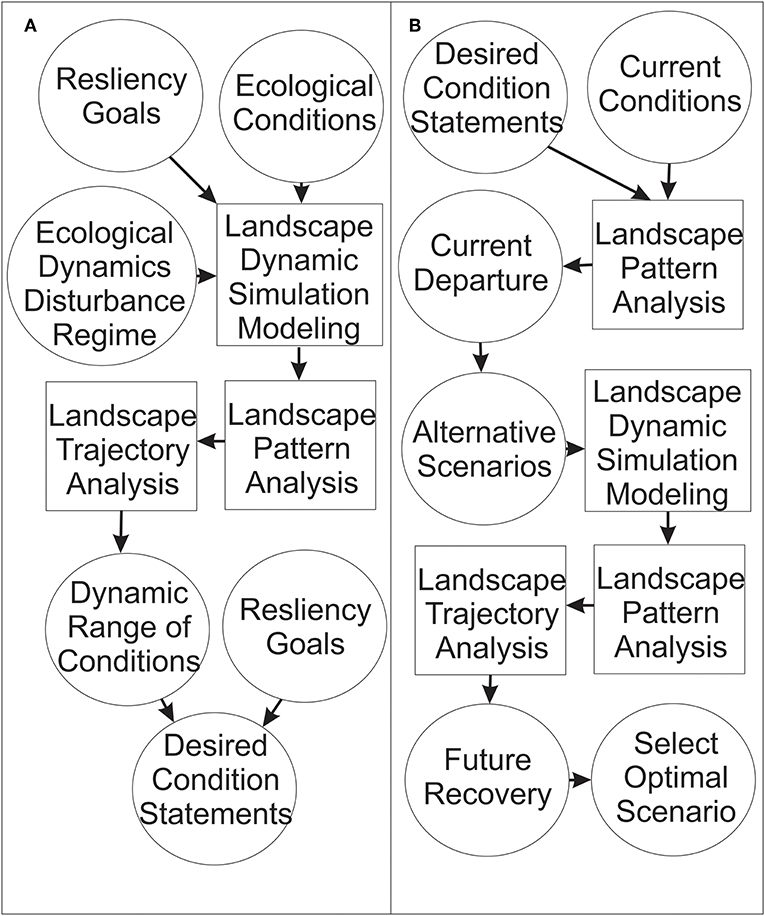
Figure 1. Conceptual diagram of applying landscape pattern analysis, landscape dynamic simulation modeling and landscape trajectory analysis to assess resiliency goals and desired conditions. Circles represent inputs or outputs of the analysis. Boxes represent analytical steps. Arrows represent linkages between inputs, analysis and outputs. (A) Shows the steps in a process of producing quantitative, detailed and specific desired conditions statements from a priori resiliency goals. (B) Shows the process of evaluating alternative scenarios given a priori detailed, specific and quantitative desired condition statements.

The example presented below combines these two approaches, by first using simulation modeling to define the dynamic range of landscape conditions expected under the historic disturbance regime, assessing the current landscape departure from that range of conditions and then evaluating how readily the landscape can return to those conditions if the historic disturbance regime were reinitiated. As noted above, this is a simplified example for heuristic purposes. In practice, managers would likely be better served by defining desired conditions based on more sophisticated assessments of resilience than historic ranges of variability, such as evaluating how a range of species, ecological conditions, and disturbance processes interact to affect system dynamics and stability. Furthermore, a more sophisticated approach to scenario evaluation should typically be used, in which a range of realistic alternative management scenarios, in the context of potentially changing climatic and disturbance drivers, interact to affect landscape conditions relative to these resilience goals (e.g., Kaszta et al., 2019). McGarigal et al. (2018) is perhaps the most complete and robust current example of combining both of these components in evaluating resilience of large forested landscapes and comparing alternative management scenarios to achieve desired conditions.

Project Area Description

The case study landscape is located in western Montana and northern Idaho, USA, and encompasses portions of the Lolo, Idaho Panhandle, and Kootenai National Forests, and the Flathead Indian Reservation. It is a logical ecological unit encompassing 1,827,400 ha and three subsections (Coeur d'Alene Mountains, St. Joe-Bitterroot Mountains, and Clark Fork Valley and Mountains) in the Bitterroot Mountains section (Figure 2).

FIGURE 2

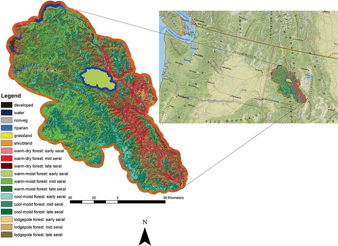
Figure 2. Study area orientation map. The case study landscape consists of a natural ecological unit in the Bitterroot Mountains of Idaho and Montana, USA (inset landscape with orange border). The Prospect Creek sub-landscape, where much of the spatial analysis is illustrated is shown as a green polygon with blue border.

There are many agents of pattern formation at the scale of the case study landscape. At more than 1.8 million hectares in size, the case study landscape contains a diverse physical environmental template, including dramatic gradients in moisture, temperature, and vegetation driven largely by variability in landform and climate. Vegetation communities and how they are distributed along environmental gradients provide the dominant source of coarse-scale landscape pattern and have a profound influence on most ecological processes and the distribution and abundance of species. Landscape dynamics in the case study landscape are driven by several coarse-scale disturbance processes such as wildfire and bark beetle outbreaks (e.g., mountain pine beetle) that interact with the physical template and each other to significantly affect vegetation patterns. Human land use patterns, past and present, also exert powerful controls on vegetation. Urban and agricultural development, largely in the low-lying valley floors, and industrial land uses such as mining and the associated transportation infrastructure (i.e., roads) create patterns that can affect the function of the landscape, in particular by disrupting habitat suitability and connectivity for wide-ranging organisms. In addition, forest management practices associated with timber harvesting and fire suppression have altered the spatial pattern of vegetation seral stages across the landscape.

Landscape Definition

The next step after defining the case study landscape is to select an appropriate landscape definition to represent patterns and their relationships to processes. This step has many important considerations (Cushman et al., 2013). Our analysis uses the landscape mosaic model (Forman and Godron, 1981), since it is by far the most commonly employed conceptual model and most landscape analysis tools use this framework. However, it is important to consider the implications of choosing the patch mosaic approach in terms of what patterns can be represented and how they can be related to driving processes. Often a gradient representation of patterns and processes can be more realistic (e.g., McGarigal and Cushman, 2005; Cushman et al., 2010), but is often limited in applicability due to lack of landscape pattern and landscape simulation tools that operate in a gradient-based framework.

Given the framework of the landscape mosaic model, we must first decide on the thematic content and resolution of the map (Buyantuev and Wu, 2007) as well as its spatial resolution (i.e., grain and minimum mapping unit; Turner, 1989; Wu, 2004). These decisions are constrained by available GIS data, the extent of the landscape, and the objectives of the analysis. There are nearly an unlimited number of variations in landscape definitions, which can have important implications for landscape analysis (Buyantuev and Wu, 2007). For heuristic purposes, we shall consider only one landscape definition in the analyses below. However, it is essential to realize that how the landscape is defined in terms of grain, extent, thematic content and thematic resolution completely controls the patterns that are measured and their relationships to underlying processes and to the concepts of resistance, resilience and recovery.

The landscape definition chosen for this analysis has the following attributes. Thematic content—The thematic content of our landscape definition is a raster map representing a patch mosaic of vegetation cover types with large streams and all roads overlaid. Thematic resolution—The thematic resolution of our land cover map is defined by the combination of two factors: (1) vegetation cover type, (2) condition, which is essentially seral stage and canopy closure. The cover type map is taken from Landfire (Rollins, 2009) and includes 22 cover types plus human development classes of road, agriculture, urban, and water. Condition has eight classes as follows: non-seral, early-all structures, mid-all structures, late-all structures, mid-closed, mid-open, late-closed, late-open. The final covercondition (covcond) map used for measuring and modeling landscape patterns therefore consists of the combination of 22 cover types at each of the eight condition classes. The spatial resolution of all raster maps is 30 m. We ran spatial filtering to specify a minimum mapping unit of patches of at least 4 cells in extent, to remove the salt-pepper effect of small and inaccurately identified patches, which can negatively impact landscape pattern analyses.

For the example analyses presented here we have chosen a subbasin within the case study landscape (Figure 3). Prospect Creek Basin is a 47,058 ha watershed in the Lolo National Forest of western Montana (Cushman et al., 2011). We chose this landscape because a regional landscape analysis of biophysical characteristics identified it as highly representative of the surrounding 1,827,400 ha comprising three subsections (Coeur d'Alene Mountains, St. Joe-Bitterroot Mountains, and Clark Fork Valley and Mountains) of the Bitterroot Mountains Ecosection. The covercondition classes used in the analyses below are the intersection of these the cover type and seral stage classifications. We show them individually here given the difficulty of interpreting maps with many classes, but it is important to keep in mind that the analysis is done on the intersection of these two, producing 22 covercondition classes.

FIGURE 3

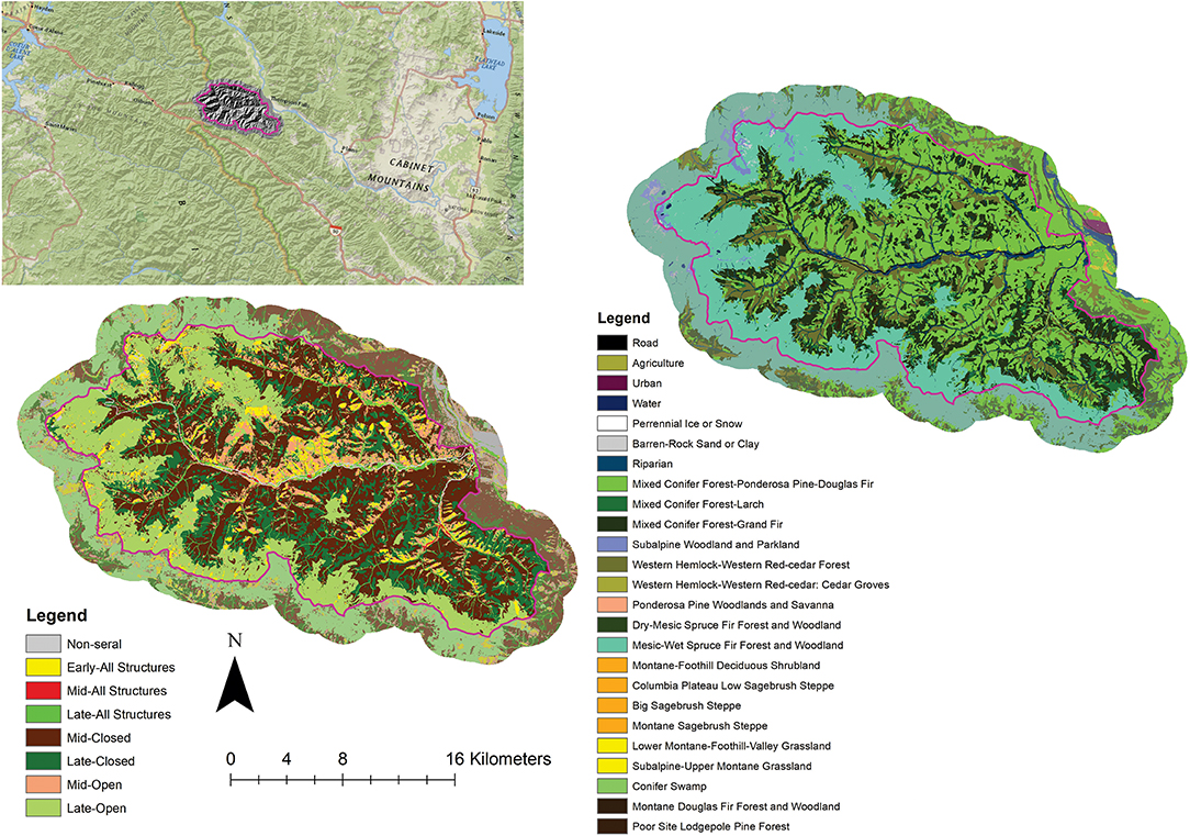
Figure 3. Prospect Creek sub-landscape. The panel in upper left of figure shows the location of the Prospect Creek watershed. The panel in the lower left shows the seral stage mosaic of the watershed, while the panel in the upper right shows the vegetation cover type mosaic of the watershed.

Measuring Landscape Pattern

The next step is to quantify landscape patterns for the case study landscape and describe its structure and composition. This step involves using the landscape pattern analysis program FRAGSTATS (McGarigal et al., 2012). Given the need for brevity, we focus on the results of this landscape pattern analysis. However, choice of landscape metrics is critically important and it is essential that researchers and managers understand metric parsimony (Cushman et al., 2008) and behavior (Neel et al., 2004), as well as how different landscape metrics may be related to ecological processes of interest, such as species distributions (Grand et al., 2004; Chambers et al., 2016) or connectivity (Cushman et al., 2012, 2013).

Landscape structure consists of several attributes measuring landscape composition (the abundance and variety of landscape elements) and landscape configuration (measuring the pattern and configuration of landscape elements). Generally, for most ecological processes landscape composition has larger effects than landscape configuration (e.g., Fahrig, 2003; Mateo-Sanchez et al., 2014). However, landscape configuration is particularly important for spatial processes, such as disturbance initiation and spread, and dispersal and colonization (Cushman et al., 2012), which are often the focus of assessments and analyses of ecological resilience. Therefore, we strongly suggest analysts consider several of the main aspects of landscape configuration (Cushman et al., 2008), such as edge contrast, patch shape complexity, aggregation, patch proximity/nearest neighbor, and large patch dominance, in addition to landscape composition. For this illustration it is not important to fully understand the intricacies of each metric. Instead, we focus on a few metrics that have intuitive interpretation.

Landscape Dynamic Simulation Modeling

The example presented here focuses on analyses of historic range of variability (HRV) of landscape structure under a natural disturbance regime, the departure of the current landscape from that range, and the degree to which return to natural disturbances could lead to recovery of resilient landscape patterns. We use a landscape disturbance-succession model (LDSMs, Mladenoff and Baker, 1999) to quantify HRV. In this paper, we present the results of the Rocky Mountain Landscape Simulator (RMLands, Cushman et al., 2011; McGarigal et al., 2018) to quantify HRV for the Prospect basin study area. Because we are using an LDSM to quantify HRV, we will refer to the “simulated range of variation” (SRV) instead of HRV to highlight the fact that our determination of HRV is based on a simulation and therefore subject to the limitations of the model.

RMLands Overview

RMLands is a grid-based, spatially-explicit, stochastic landscape simulation model designed to simulate disturbance and succession processes affecting the structure and dynamics of Rocky Mountain landscapes. RMLands simulates two key processes: succession and disturbance. These processes are fully specified by the user via model parameterization and are implemented sequentially within user-specified time steps for a user-specified period of time. Succession occurs at the beginning of each time step and represents the gradual growth and/or development of vegetative communities over time. Succession is implemented using a stochastic state-based transition approach in which vegetation cover types transition probabilistically between discrete states (conditions). Transition pathways and rates of transition between states are defined uniquely for each cover type and are conditional on several attributes of a vegetation patch.

Model Characteristics

RMLands can be classified as a hybrid statistical/probabilistic model with the following distinguishing characteristics: (1) RMLands utilizes a grid-based data model in which the landscape is represented in a regular grid lattice structure. Each grid cell (pixel), representing a fixed geographic area, possesses a number of ecological attributes (e.g., cover type, age). Attributes possess multiple states (i.e., unique values), many of which change over time in response to succession and disturbance. (2) Consistent with the grid structure, RMLands is a spatially-explicit model; grid cells are geographically explicit and topological relationships are important in all processes (e.g., disturbance initiation and spread). (3) RMLands is a process-based model and simulates both disturbance and succession. Disturbance processes include a variety of both natural and anthropogenic disturbances that are implemented in a common fashion. Succession is based on a discrete state transition model for each cover type. (4) RMLands is a stochastic model. Each cell has a probability of initiation for each disturbance process that is contingent on several cell attributes. Thus, given the same cell attributes, some cells will initiate while others will not. There is a stochastic element to nearly all processes in RMLands. (5) The grid can be defined at any spatial resolution, although current applications utilize a relatively high resolution (25–30 m cell size) grid that allows for detailed representation of landscape patterns. In addition, while RMLands does not limit the extent of the landscape, it is most applicable to landscapes between 10,000's ha to over 1 million ha. (6) RMLands operates on a user-specified time step and is most applicable to simulating landscape dynamics over 100's to 1000's of years.

Steps of Assessing SRV and Current Departure Relative to Ecological Resilience

This example focuses on using landscape pattern analysis and landscape dynamic simulation modeling to evaluate the resilience of a case study landscape. The evaluation is based on quantifying current landscape structure and comparing it to the ranges of landscape patterns simulated under a natural, historical disturbance regime. The link to resilience is the idea that the structure of the landscape (composition and configuration) that emerged under the natural historic disturbance regime reflects the dynamics of the landscape under regulation by natural processes and the conditions under which ecological processes and species existed prior to perturbation by human influences. The assessment example is presented in five steps, which are described below.

Step 1. Establish the Objective of the Analysis

The first step is to establish the objective of the analysis. Our overall objective is to quantify HRV for the sample landscape and compare the current landscape departure from it to assess some aspects of ecological condition relevant to resilience, and evaluate how readily the landscape can recover from this departure if the natural disturbance regime were reimposed, as a measure of recovery. We focus on three questions: (1) What is the historic range of variation in landscape structure in the sample landscape? (2) What is current degree of departure of the current landscape condition from that historic range of variability, and how do these things change with the spatial scale (extent) of the landscape under consideration? (3) How readily does the landscape pattern recover to within the HRV after the reimposition of the historic disturbance regime.

For the purpose of this example we define “historic” as the period from about 1300 to the late 1800s, representing a period of largely indigenous settlement. This period represents a time when broad-scale climatic conditions were generally similar to those of today, but Euro- American settlers had not yet introduced the sweeping ecological changes that now have greatly altered many Rocky Mountain landscapes. Moreover, it was a time of relatively consistent (though not static) environmental and cultural conditions in the region, and a time for which we have a reasonable amount of specific information to enable us to model the system.

Step 2. Define the Digital Landscape

The next step is to define the digital landscape. We selected a single sample landscape (Prospect Creek Subbasin), from the entire case study landscape based on the following criteria: (1) landscape extent large enough to incorporate meaningful landscape dynamics given the scale of the major disturbance processes, yet small enough to be computationally efficient for lab use, (2) representativeness of the major land cover patterns found throughout the entire case study landscape; in particular, focusing on adequate representation of the four dominant forest cover types, (3) a heterogeneous mixture of land use practices, including developed lands with a wildland-urban interface, a mixture of public and private lands dominated by the former, and an adequate road network to facilitate future vegetation treatments, and (4) a logical ecological unit, in this case, a watershed, meeting the above criteria. Based on these criteria, we selected Prospect Creek basin, a 47,058 ha watershed located roughly in the center of the case study landscape (Figure 3).

We classified the sample landscape into land cover classes based on the LANDFIRE project (Rollins, 2009). Specifically, land cover classes represent unique biophysical settings (BpS) or potential vegetation types (PVT). The only significant change we made to this classification scheme was to combine three separate BpS classes corresponding to “riparian” settings into a single “riparian” class. The spatial grain (or resolution) of the landscape was set at 30 m, consistent with the spatial resolution of the data sources used in the LANDFIRE project. The spatial extent of the landscape was based on the hydrological watershed of Prospect Creek, a tributary of Clark Fork River; however, for simulation purposes we included a 2-km wide buffer zone around the basin, bringing the total extent of the simulation landscape to 69,293 ha.

Step 3. Run the RMLands Simulation and Quantify the Structure of the Simulated Landscapes Using FRAGSTATS

The next step is to parameterize and run the RMLands simulation and then parameterize and run FRAGSTATS to quantify the structure of the simulated landscapes. RMLands parameterization generally involves extensive research and expert team meetings, and can take weeks to years to complete. To illustrate this example we ran a 2,000 year (200 10-year timestep) simulation. We selected a broad range of class- and landscape-level metrics, including both structural and functional metrics, to assess landscape structure produced by the simulation.

Step 4. Examine the Model Equilibration

The next step is to examine the model equilibration. We must first characterize HRV under dynamic equilibrium conditions in which the landscape fluctuates within a stable range of variation. Because the current landscape may not be operating within its HRV, it is usually necessary to allow the simulated landscape to “return” to its stable SRV. Consequently, there is usually an “equilibration period” at the beginning of the simulation during which the landscape adjusts to equilibrium conditions. Here, we will examine the magnitude and duration of the model equilibration. There is no simple way to quantify the existence and length of the equilibration period, so it is usually determined subjectively by examining the simulated trajectory of landscape change. There are several possible descriptive statistics that could be evaluated to assess the equilibration period. For pragmatic reasons, here we will consider only two.

Seral-Stage Distribution

In this section we consider the dynamics in the seral-stage distribution for each cover type. We first examine the cover-condition dynamics plots for evidence of a model equilibration period—a period at the beginning of the simulation during which the seral stage distribution is noticeably different from the remainder of the simulation. Note, it would be prudent to pay attention to only those cover types with substantial area in the simulation landscape (Table 1), since the dynamics for the poorly represented cover types can be unreliable or uninformative.

TABLE 1

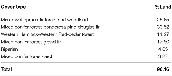
Table 1. Percentage of the Prospect Creek Basin case study landscape in each of the major cover types.

There is a distinct model equilibration period in landscape composition that is evident in all cover types, as illustrated in the example below in the seral-stage distribution of mixed conifer forest-ponderosa pine-Douglas fir cover type (Figure 4). Based on the majority of metrics, the equilibration period is roughly 200 years, but a few metrics don't equilibrate until after 500 years.

FIGURE 4

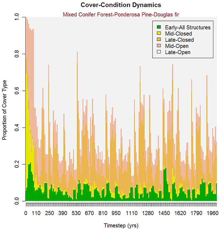
Figure 4. Temporal plot of proportion of the Prospect Creek landscape covered by each of the different seral stages for one focal vegetation cover type, Mixed Conifer Forest - Ponderosa Pine-Douglas Fir.

There is considerable variation in the equilibration period among cover types, as illustrated by the differences between mesic-wet spruce-fir forest and woodland (MW_SF, Figure 5) and mixed conifer forest-ponderosa pine-Douglas fir (MCF_PPDF). In general, the equilibration period is relatively short, in the range of 100–150 years, for the ponderosa pine type, but considerably longer, up to 500 years, for the spruce-fire type. The differences between these cover types are likely due to dramatic differences in their characteristic disturbance regimes. The ponderosa pine type is subject to very frequent wildfires (mean fire return interval of roughly 25 years), while the spruce-fir type is subject to infrequent disturbances (mean fire return interval of roughly 200 years). The frequent disturbances in the ponderosa pine type allows the system to equilibrate rather quickly in contrast to the slow dynamic of the spruce-fir type.

FIGURE 5

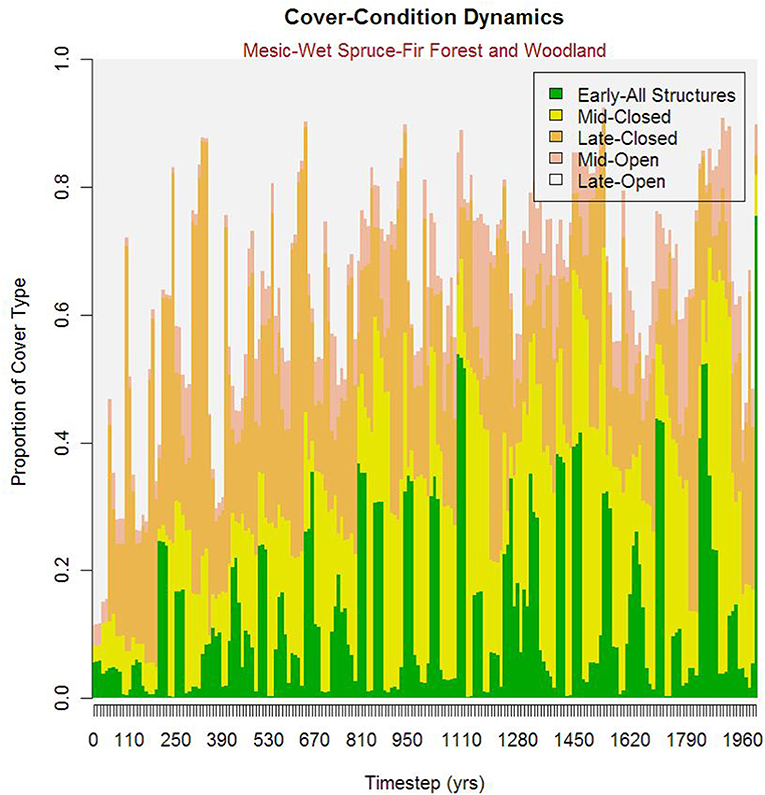
Figure 5. Temporal plot of proportion of the Prospect Creek landscape covered by each of the different seral stages of one focal vegetation cover type, Mesic-Wet Spruce-Fir Forest and Woodland.

Landscape Structure

The next step is to consider the dynamics in landscape structure based on the FRAGSTATS landscape-level metrics. First, we determine if there is a detectable model equilibration period in landscape structure based on the FRAGSTATS landscape-level metrics and estimate what that period is. We evaluate how this equilibration period differs among landscape metrics and identify the aspects of landscape structure that appear to be most in need of model equilibration.

There is a distinct model equilibration period in landscape structure, but it is highly variable among landscape metrics. Some metrics show a distinct model equilibration period, while others exhibit essentially no model equilibration. This indicates that some aspects of the current landscape structure are within the simulated range of variability, while others are not. In particular, the landscape metrics associated with the large patch structure (e.g., GYRATE_AM, LPI, CONTAG, Figures 6A–C), specifically the size and extensiveness of the large patches, are most in need of model equilibration. That is to say, the large patch structure in the current landscape departs the most from the SRV. In addition, the interspersion and juxtaposition index and Shannon's and Simpson's landscape diversity indices all exhibit a distinct model equilibration, indicating that the diversity of the current landscape also deviates considerably from the SRV. This result is consistent with the findings from the cover-condition statistics that indicate that most cover types have a current seral-stage distribution that deviate from their SRV. In contrast, many aspects of landscape structure, in particular edge density and edge contrast, do not require any model equilibration and are thus currently within their SRV. In general, with the exception of SHAPE_AM, the landscape metrics requiring equilibration do so rather quickly, mostly within 100 years.

FIGURE 6

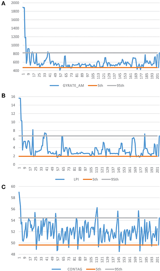
Figure 6. Temporal plot of three landscape metrics within the Prospect Creek landscape. (A) Correlation Length (Gyrate_AM), (B) Largest Patch Index (LPI), (C) Contagion (CONTAG). The blue line represents the value of the landscape metric over the simulation time. The gray line is the upper 95th percentile of the simulated range, and the orange line is the lower 5th percentile of the simulated range.

Step 5. Evaluate the Simulated Range of Variability in Landscape Structure and Current Departure for Individual Metrics

Seral-Stage Distribution

A tabular summary of SRV in cover-condition (i.e., cover type seral-stage distribution) provides a simple means to evaluate the departure of the current condition from SRV. Given the large number of covercondition classes in this analysis, here we present only a subset of a few cover types of particular interest for this analysis. These include mixed-conifer, ponderosa pine-Douglas fir, early seral (MCF_PPDF_e), mixed-conifer forest, ponderosa pine-Douglas fir, late seral open canopy (MCF_PPDF_lo), and mesic-wet spruce-fir, late seral open canopy (MW_SF_lo). Table 2 provides a summary of the simulated range of variability in the distribution of area among condition classes (i.e., seral stages) for these cover types and the departure of the current landscape from the simulated range of variability for each condition class, the current value of the metric, and a summary of the computed cover type departure index (CDI). This index represents the overall departure of a cover type from the simulated range of variability in the distribution of area among condition classes. The table also includes how many standard errors the current condition is from the mean of the simulated distribution (stderr), and the percentile the current condition is of the range of the simulated distribution (pct_srv).

TABLE 2

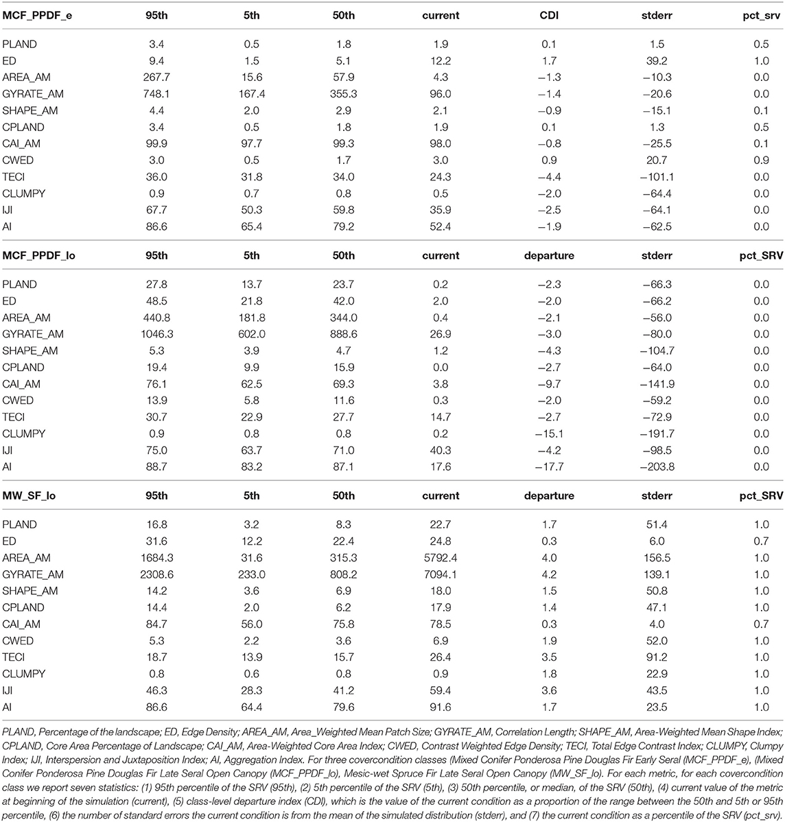
Table 2. Simlulated range of variability of 12 class-level landscape metrics.

We can use the information in these tables to evaluate the range of variability and departure of the current landscape composition from the SRV for the three covercondition classes listed above. We choose to quantify the SRV (HRV) based on the 5th and 95th percentiles of the simulated distribution in the percentage of the cover type comprised of each seral stage. The 5th−95th percentiles capture almost the full range of variability without being overly sensitive to extremes. Based on this we see, for example, the SRV for PLAND of MCF_PPDF_e is from 0.5 to 3.4% and the median value of the SRV is 1.8%. Similarly the SRV for PLAND of MCF_PPDF_lo is 13.7 to 27.8% and the median is 23.7%. Finally, for MW_SF_lo the SRV of PLAND is 3.2 to 16.8% with a median of 8.3%. There is not sufficient space in this paper to discuss or elaborate on the SRV results for all the classes or all the metrics, but one could compute and compare SRV, current value and departure for all metrics for all covercondition classes to identify the attributes that are most departed from SRV and in what way they are perturbed from the range expected.

Table 2 also contains several measures of the current departure from the range of variability (SRV) for the amount of the landscape in each cover-condition class. There are many ways we could represent the degree of departure. This table shows three: (1) cover type departure index (CDI), ranging from 0 (no departure) to maximum (current value as a proportion of the range between median-95% confidence limit), (2) standard errors of current from distribution of SRV, (3) percentile of SRV. Focusing again on the PLAND metric for the three coverconditoin classes, we see that for MCF_PPDF_e we have a DPI of 0.1 indicating that the current value is larger than the median by 10% of the range between the median and 95th percentile. This indicates the value is well within the SRV. Different measures of the same thing are given by stderr and pct_srv, which show, respectively, that the current PLAND for this covercondition class is 1.5 standard errors above the mean of the simulated distribution and that the current value is 50th percentile of the SRV. Conversely, for MCF_PPDF_lo we see the CDI value is −2.3, indicating that the current value is lower than the median by 2.3 times (230%) the range from the median to the 5th percentile. The stderr and pct_SRV also show strong departure, with values of −66.3 and 0, respectively, indicating that PLAND of MCF_PPDF_lo in the current landscape is much lower than the range expected by the SRV. Likewise, for MW_SF_lo the current PLAND of 22.7% has a departure index (CDI) of 1.7, a stderr of 51.4 and pct_SRV of 1.0, indicating that the current extent (PLAND) of late open spruce fir is much greater than the range of the SRV.

Landscape Structure

In addition to range of variation and departure of amounts and configuration of each covercondition class, we are often interested in examining SRV in landscape structure and current departure based on the FRAGSTATS landscape-level metrics. The structure of Table 3 is very similar to that of the covcond table above, the only difference being that instead of unique cover-condition classes (rows), we have landscape metrics which measure the composition and configuration of the entire landscape mosaic of multiple covercondition classes simultaneously. The landscape departure index (LDI) is computed in the same manner as the cover type departure index (CDI) and represents the average departure among landscape metrics from the SRV. Likewise, the standard errors from the mean of the SRV distribution and percentile of the SRV distribution are calculated the same way as well.

TABLE 3

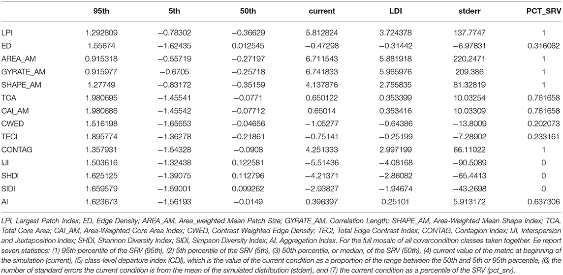
Table 3. Simlulated range of variability of 16 landscape-level metrics.

We can use the information in Table 3 to identify what aspects of landscape structure exhibit the greatest SRV (not departure). Specifically, the large patch structure, specifically the size and extensiveness of the large patches and overall clumpiness of the landscape (AREA_AM, GYRATE_AM, CONTAG), exhibits the greatest SRV. Essentially, under natural dynamic conditions the coarse patch structure of the landscape fluctuates dramatically in response to coarse scale disturbances followed by succession. Large, contiguous patches of, for example, mature high-elevation spruce-fir forest are occasionally broken up by infrequent large disturbance events, generally a wildfire or mountain pine beetle outbreak, only to be followed by long periods of succession during which disturbance patches succeed and eventually coalesce to form large extensive patches again.

Table 3 also contains several measures of the current departure from the range of variability (SRV) for structure and composition of the covercondition class mosaic. For example, the landscape departure index (LDI), ranging from 0 (no departure) to maximum (current value as a proportion of the range between median-95% confidence limit) shows that the current landscape structure departs greatly from the SRV for 8 metrics, listed here in order of decreasing departure: GYRATE_AM, AREA_AM, IJI, LPI, CONTAG, SHIDI, SHAPE_AM, SIDI. The sign of these LDI scores indicates that the current landscape is much more aggregated (CONTAG, IJI), with large and more extensive patches (AREA_AM, GYRATE_AM, LPI), which are much more complex in shape (SHAPE_AM) that would be expected under the SRV. In contrast, several other metrics are not departed from the SRV, including ED, CWED, TECI, which indicates that the amount of total edge and edge contrast in the landscape is within the SRV. Standard errors of current from distribution of SRV and percentile of SRV echo the LDI in terms of the relative departure of the different metrics.

Conducting this evaluation shows that current departure is very sensitive to the choice of metric. For example, the cover type departure indices derived from the seral-stage distribution data (covcond) vary greatly for the cover types with significant area in the Prospect Creek landscape. Similarly, the landscape departure indices based on individual landscape structure metrics range similarly widely. For example, the aggregation index (AI) at the landscape level has a departure index of 0.23, indicating the current condition is well within the range of the SRV. In contrast, correlation length (GYRATE_AM) at the landscape level has a departure index of 5.97 because the current landscape condition is exceeds the 95th percentile of the SRV by 5.97 times the range from the median to the 95th percentile. Thus, the choice of metric can lead to opposite conclusions regarding the departure of the current landscape. For this reason, a multivariate approach is necessary, whereby several metrics are evaluated together.

Multivariate Trajectory Analysis

Landscape-Level Landscape Multivariate Trajectory Analysis

We implemented a landscape trajectory analysis (sensu Cushman and McGarigal, 2007) with multi-temporal principal components analysis (e.g., Cushman and Wallin, 2000) to show the main pattern among landscape-level metrics (e.g., FRAGSTATS; McGarigal et al., 2012) across the 200 time steps of the simulation (Figure 7). The PCA was done on a table of centered and standardized values of 14 landscape-level metrics: ED, edge density; CWED, contrast-weighted edge density; TECI, total edge contrast index; SHDI, Shannon diversity index; IJI—interspersion and juxtaposition index; SIDI, Simpson diversity index; AI, aggregation index; TCA, total core area; CAI_AM, area-weighted core area index; CONTAG, contagion; GYRATE_AM, area-weighted mean patch radius of gyration; LPI, largest patch index; AREA_AM, area-weighted mean patch size; SHAPE_AM, area-weighted mean patch shape index.

FIGURE 7

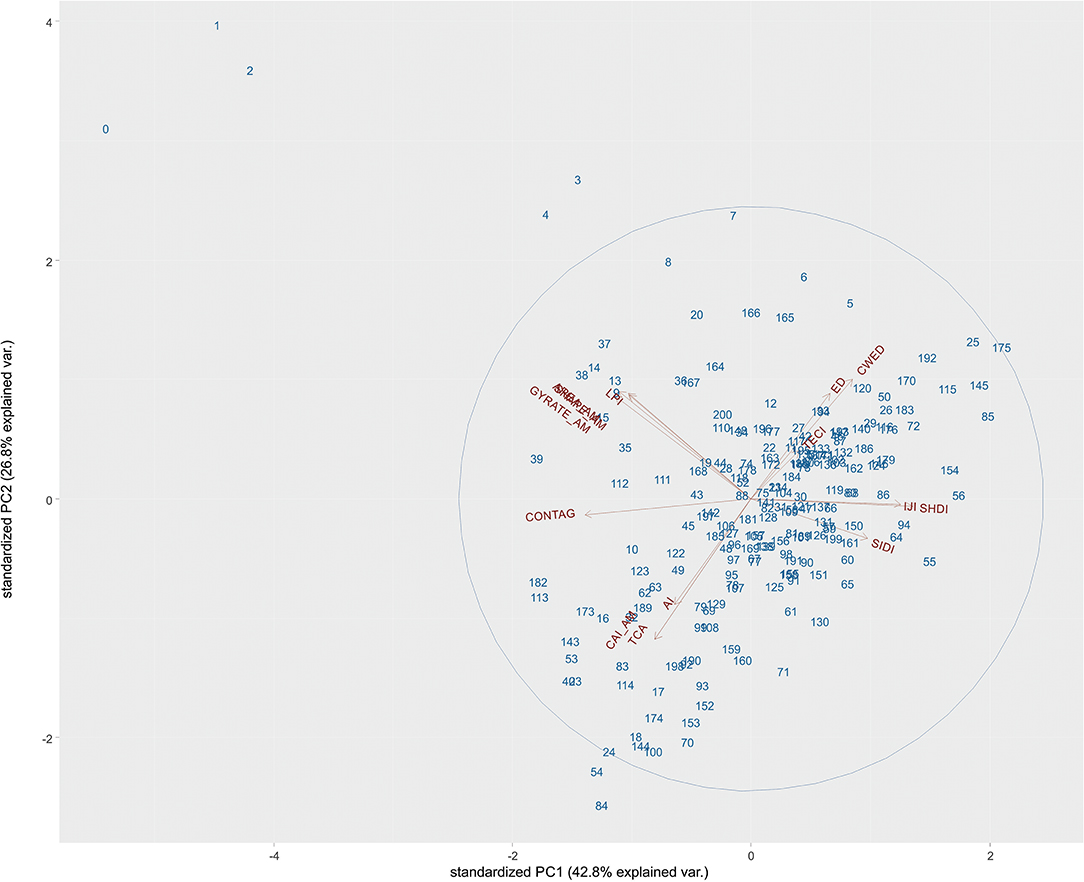
Figure 7. Multi-temporal principal components plot of landscape-level metrics in the Prospect Creek watershed across the simulation time. Blue numbers represent landscape conditions at each time step, which represent years of simulation/10. The blue ellipse contains 95% of the simulated range in principal components space. The red vectors represent the direction of change in each of the landscape metrics, whose acronyms are shown at the end of each vector. AI, Aggregation Index; TCA, Total Core Area; CAI_AM, Area-weighted Core Area Index; CONTAG, Contagion; GYRATE_AM, Correlation Length; AREA_AM, Area-weighted Mean Patch Size; LPI, Largest Patch Index; ED, Edge Density; CWED, Contrast-weighted Edge Density; IJI, Interspersion and Juxtaposition Index; TECI, Total Edge Contrast Index; SHDI, Shannon's Diversity Index; SIDI, Simpson's Diversity Index.

The first two axes explain 70% of the total variance in class-level landscape structure, with the first axis explaining 43% and the second 37%. The first axis is highly aligned with CONTAG, IJI and SHDI. CONTAG increases to the left, and IJI and SHDI increase to the right, indicating that the right represents a more heterogeneous condition with lower aggregation, higher diversity of patches and higher interspersion of patches, while the left indicates conditions where there is high homogeneity and aggregation of the landscape. The second axis is associated with patch interspersion, and edge contrast, with highest patch interspersion and edge contrast to the top of the axis. The black ellipse on the plot indicates the 95^% probability ellipse for all points in the plot. The red vectors point in the direction of increasing value of each metric. For example the upper right quadrant of the PCA is areas with high edge density, low core area, low aggregation, and high edge contrast. The lower left quadrant is the opposite: conditions characterized by high landscape aggregation, high core area, low edge density and low edge contrast. The upper left quadrant is represented by extreme conditions associated with very high largest patch size, very high area-weighted mean patch size, and very high area-weighted mean patch radius of gyration. This represents conditions with very large and very extensive patches.

The numbers on the graph represent the time step in the simulation. The location of the time steps across the PCA space shows the trajectory of change in multi-variate landscape structure from the current (initial) condition (0) to the end of the simulation (200). The current condition is far to the upper left, indicating that the current landscape has much larger, more extensive, and more connected patches than expected under the SRV. The distance from the initial condition (0) to the centroid of the PCA (which is 7.4 PCA axis units in this case) is a measure of departure from the center of the SRV, and the distance from the boundary of the 95% ellipse (4.9 in this case) is a measure of the departure from the SRV range. The ratio of these, 8.4/4.9, or 1.71, indicates how far the current value is beyond the SRV ellipse in terms of the width of the SRV ellipse. This means that the current multivariate LDI index is 1.71, given that the current condition is 1.71 times farther from the centroid of the PCA than the full width of the SRV condition.

During the simulation, the landscape condition returns to within the SRV (95% ellipse) within 5 time steps (50 years). There is considerable dynamic variation in landscape structure over the simulation time, with some quasi-periodic fluctuation between upper right (high edge density and low core and contagion) and lower left (low edge density and high core and contagion). However, never in the simulation time does the condition of the landscape approach anything like the initial (current) condition, which is characterized by very large, highly connected and extensive patches with low diversity. The current condition is far outside the SRV, but the patterns change relatively quickly over the simulation time to return to within the 95% ellipse, showing relatively rapid recovery once the historic disturbance regime is reestablished.

Class-Level Landscape Multivariate Trajectory Analysis

We again used multi-temporal principal components analysis (e.g., Cushman and Wallin, 2000) to show the main pattern among cover-condition classes across the 200 time steps of the simulation (Figure 8). The PCA was done on a table of centered and standardized values of 12 class-level metrics: TECI, total edge contrast index; IJI, interspersion and juxtaposition index; CAI-AM, area-weighted core area index; CLUMPY, clumpy index; AI, aggregation index; CWED, contrast-weighted edge density; CPLAND, core area percentage of the landscape; PLAND, percentage of the landscape; ED, edge density; GYRATE_AM, area-weighted mean radius of gyration; AREA_AM, area weighted mean patch size; SHAPE_AM, area-weighted shape index. The first two axes explain 85% of the total variance in class-level landscape structure, with the first axis explaining 51% and the second 34%. The first axis is highly aligned with PLAND and CPLAND, with these metrics increasing to the right. This axis is associated with very extensive cover types to the right and low extent of the cover types to the left. The second axis is highly associated with patch interspersion, and edge contrast, with highest patch interspersion and edge contrast to the top of the axis. The black ellipse on the plot indicates the 95% probability ellipse for all points in the plot. The red vectors point in the direction of increasing value of each metric.

FIGURE 8

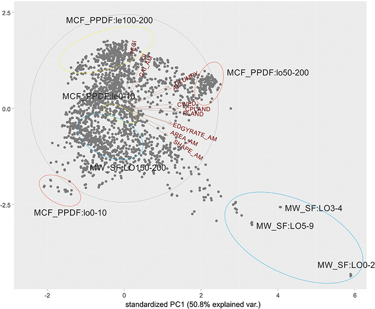
Figure 8. Multi-temporal principal components analysis of class-level metrics in the Prospect Creek watershed across the simulation time. Gray dots are combinations of cover type at a given seral stage at a given simulation time step. The gray ellipse contains 95% of the simulated range in landscape structure space. The red vectors represent the direction of increase of each landscape metric and metric acronyms are labeled at the end of each vector. The blue ellipses show cover-seral conditions for two cover types (Mixed-Conifer Ponderosa Pine-Douglas Fir Late Seral Open Canopy - NCF_PPDF; Mesic-Wet Spruce-Fir Late Seral Open Canopy - MW_SF) at early and late simulation times. Simulation times are indicated by the numbers at the end of the acronym. For example, MCF_PPDF:lo0-10 ellipse encloses the initial condition and first ten time steps of the Mixed-Conifer Ponderosa-Pine Douglas Fir Late Seral Open Canopy cover-seral class in landscape structure space. TECI, Total Edge Contrast Index; IJI, Interspersion and Juxtaposition Index; CAI_AM, Area-weighted Core Area Index; CLUMPY, Clumpy Index; AI, Aggregation Index; CWED, Contrast Weighted Edge Density; CPLAND, Core Area Percentage of the Landscape; PLAND, Class Percentage of the Landscape; ED, Edge Density; GYRATE_AM, Correlation Length; AREA_AM, Area-weighted Mean Patch Size; SHAPE_AM, Area-weighted Shape Index.

The points on the graph indicate the locations of each cover type at each time-step in the landscape structure space. To illustrate the temporal change in landscape structure in a few key landcover types we have located and labeled the initial and ending locations of four cover-condition classes: MW_SFlo—mesic-wet, spruce-fir, late seral, open canopy; MCF_PPDF:lo—mixed conifer forest, ponderosa pine, Douglas fir, late seral, open canopy; MCF_PPDF:e—mixed conifer, ponderosa pine, Douglas fir, early seral. The change in conditions over the simulation time is illustrated by the movement of the points for that cover-condition class across these two-dimenions of the PCA. For example, MW_SF:Lo (blue ellipses) starts far to the right of axis 1 and bottom of axis 2, with conditions characterized by very high extent (percent of the landscape) and very large patch size (AREA_AM, GYRATE_AM). This indicates that at the beginning of the simulation (current condition), the landscape is highly dominated by large, complexly shaped patches of mesic-wet late seral open canopy spruce fir. This structure is far outside the 95% ellipse of the simulated range (SRV), indicating the current condition of the landscape departs substantially from expected under the historic disturbance regime. At the end of the simulation time (which represents the simulated range of conditions under the historic disturbance regime), this cover-condition class has moved toward the left of axis 1 and somewhat below the center on axis 2. This indicates that under the simulated historical disturbance regime mesic-wet spruce fir late seral open canopy class would likely exist in relatively moderate extent, with much smaller and simpler shaped patches than in the current condition.

In contrast to MW_SF:Lo, which our simulation predicts is more extensive than expected under the SRV, MCF_PPDF:Lo shows the opposite response. Specifically, at the beginning of the simulation mixed conifer ponderosa pine, Douglas fir, late seral open canopy is the farthest to the left on axis 1 of any cover-condition class, indicating very low extent and small patches. During most of the simulation, however, this cover-condition class moves far to the right on axis 1 and up on axis 2, such that under the SRV it is expected to be the most extensive cover type, with the largest and most complex shaped patches.

The same exercise could be repeated for each cover-condition class, calculating the distance in PC space (e.g., displacement, Cushman and McGarigal, 2007) from the initial condition to the centroid of the distribution of the SRV or the 95% ellipse. Making this calculation we see that MW_SF:Lo and MCF_PPDF:Lo are the two cover-condition classes that are most departed from multi-variate class-level pattern in their current condition compared to the SRV, with late-open spruce fir much more extensive and late-open ponderosa pine, Douglas fir much less extensive than expected under the SRV. Given landscape patterns are inherently multivariate, this kind of analysis using multi-temporal PCA across the full simulation time is more informative and comprehensive, although less intuitive, than looking at plots for individual metrics for individual cover-condition types. The number of time steps it takes the simulation to change the landscape structure for each cover-condition type to within the SRV, or 95% ellipse, is a measure of the amount of time needed for recovery of landscape patterns once a historical disturbance regime is re-established. From this we see it takes a different amount of time for MW_SF:Lo (~150 years) than for MCF_PPDF:Lo (~60 years). This shows that the departure of MW_SF:Lo from SRV is not only larger (e.g., distance in PCA space), but less responsive for recovery (time to return within the SRV).

Discussion

A resilience-based management approach facilitates regional planning by providing evaluations of current ecological conditions relative to system equilibrium and reference states (Hessburg et al., 2013; McIntyre et al., 2014; Tambosi et al., 2014; Rappaport et al., 2015; Chambers et al., 2019). Importantly, operationalizing the concept of resilience into an analytical framework enables the optimization of management actions to achieve have the greatest benefits (e.g., McGarigal et al., 2018). Chambers et al. (2019) reviewed six key components of a resilience-based approach, including (1) formalizing the concept of managing for adaptive capacity, (2) selecting an appropriate spatial extent and grain, (3) understanding the factors influencing the resilience of ecosystems and landscapes, (4) the importance landscape context in measuring and defining resilience, (5) pattern and process interactions and their variability, and (6) relationships among ecological and spatial resilience and the capacity to support habitats and species. The purpose of this paper is to provide an introduction to concepts and methods from landscape ecology to implement these six components of assessing and managing for ecological resilience.

A spatially explicit approach coupling geospatial information on ecological system characteristics and disturbance provides the foundation for resilience-based management. Landscape ecology is the science of pattern-process relationships and, in particular, how patterns of disturbance, recover and ecological conditions drive ecological processes (Turner, 1989). The tools of landscape ecology, including landscape pattern analysis and landscape dynamic simulation modeling provide a means to implement the six components of the ecological resilience framework (Chambers et al., 2019). In this paper we provide a case study landscape of using landscape pattern analysis (e.g., McGarigal et al., 2012) and landscape dynamic simulation modeling (e.g., Littell et al., 2011; McGarigal et al., 2018) to assess the ecological condition of a case study landscape and how the current condition of that landscape departs from the range of conditions expected under a historic disturbance regime.

In this example (1) we formalize the concept of managing for adaptive capacity under the framework of assessing current conditions relative to the range of conditions expected under a natural disturbance regime, which can subsequently be used to optimize management scenarios to best achieve resilient landscape conditions (e.g., McGarigal et al., 2018). Our example focuses on (2) developing a meaningful and appropriate landscape definition for analysis, including decisions regarding grain, extent, thematic content and thematic resolution. This is critical, as all pattern-process relationships, including assessments of resilience, depend on correctly defining the landscape relative to the dominant ecological characteristics and the drivers that affect their value and dynamics (Wu, 2004; Buyantuev and Wu, 2007). We assess (3) factors affecting the resilience of ecosystems and landscapes in this case study by focusing on the processes of how natural disturbance regimes interact with topography, climate and vegetation to driver patterns of ecosystem structure (Romme and Knight, 1981). The use of a spatially explicit, dynamic landscape simulation model (Mladenoff and Baker, 1999; Costanza and Voinov, 2004) allows (4) assessment of the landscape context in evaluating resilience. Specifically, in this case our simulation of the expected range of ecological conditions under a natural disturbance regime provides a framework for evaluating the current condition relative to the range of conditions the system would exist in without human perturbation. This provides the key reference framework for evaluating current conditions relative to measures of ecological resilience, including degree of departure from reference conditions (simulated range of natural variation), and ability of the system to recover (how rapidly it reenters the range of simulated range of variability once a natural disturbance regime is reestablished. This framework is formally based on (5) evaluating pattern-process interactions (Turner, 1989) and their variability, which is a key component of defining, measuring and managing for ecological resilience. Finally, (6) the assessment we provide can be linked to assessing the relationship between landscape patterns and particular ecological processes, such as maintenance of habitats and species (e.g., Cushman et al., 2011). For example, Cushman and McGarigal (2007) used the RMLands model to simulate several alternative forest management scenarios and coupled them to multi-scale habitat relationships modeling for a focal species (American marten, Martes americana) and used multivariate landscape trajectory analysis to quantify the relative impacts of different forest harvest regimes on the extent, pattern and trajectory of change of habitat for this forest dependent species. Similarly, Cushman et al. (2011) used RMLands and multi-scale habitat modeling to project the effects of climate change, forest restoration treatments and fire suppression on habitat extent and pattern of two focal species (American marten and flammulated owl) in the Prospect Creek case study landscape. That analysis showed that forest restoration treatments, at levels realistic given management and logistical constraints, are unlikely to greatly affect wildfire disturbance regimes and that climate driven changes in fire regimes likely will decrease habitat quality for the closed-forest dependent American marten, but are less likely to severely affect habitat quality for the open-canopy specialist flammulated owl.

The case study example in this paper focuses on a particular watershed in the U.S. Northern Rocky Mountains and measures how the current landscape composition and configuration differ from the expected range under a natural disturbance regime. The example is intended to be heuristic and illustrative of the ideas, methods and tools used by landscape ecologists to assess current conditions relative to reference conditions. In this case we defined the landscape based on a patch mosaic model with cover types defined by combinations of dominant vegetation type, stand age and canopy closure. This choice of landscape definition fundamentally affects all analyses, results and interpretation. We do not propose that this particular landscape definition is ideal for all, or even any, particular applications. We chose since it is intuitively familiar to most managers and scientists, and since many tools we utilize employ a patch mosaic framework (e.g., FRAGSTATS, McGarigal et al., 2012, RMLANDS, McGarigal et al., 2018), and because many past assessments of landscape effects on ecological processes have used similar landscape definitions (e.g., Cushman and McGarigal, 2007; Cushman et al., 2011; McGarigal et al., 2018).

We illustrate the use of landscape pattern analysis with FRAGSTATS (McGarigal et al., 2012) as a means to quantitatively measure the spatial attributes of landscapes over time and across space. The ability to comprehensively and quantitatively evaluate and compare ecological conditions across space and time is essential to measure the characteristics of current conditions and compare them to reference frameworks of other landscapes or dynamic ranges under historic disturbance regimes (e.g., McGarigal et al., 2018), or to outcomes of simulated alternative future scenarios (e.g., Kaszta et al., 2019). Landscape pattern analysis is a foundational idea in landscape ecology and is a powerful tool to measure and evaluate ecological conditions in the context of ecological resilience. In our example we illustrated this by using FRAGSTATS to measure a number of spatial attributes of the case study landscape, which collectively quantified many attributes of its composition and configuration which we chose based on their utility in describing major gradients of landscape structure (e.g., Cushman et al., 2008), and their known associations with many ecological processes (e.g., Grand et al., 2004; Chambers et al., 2016).

We used spatially-explicit dynamic landscape simulation modeling with RMLANDS to provide a spatio-temporal reference framework for assessing some aspects of ecological resiliency. Landscape dynamic simulation modeling is extremely useful to project the dynamic range of conditions one would expect under different scenarios of disturbance, succession, management and climate. A reference framework to compare current conditions against quantitatively is an essential foundation for any rigorous assessment of resilience. Reference frameworks can be constructed by comparing focal landscapes to other landscapes which have particular reference characteristics (e.g., comparing managed or disturbed landscapes to those in protected areas such as Wilderness), or to the distribution of all landscapes in the study region (e.g., how does the focal landscape compare to the range of conditions more broadly). These approaches in a sense “trade space for time” by assuming that the current conditions of the reference landscapes reflect some important aspects of the past conditions of the reference landscape, relevant for assessing resilience. There are strengths and weaknesses of that approach. The strength is it is comparing real current conditions to real actual conditions in reference landscapes, which removes uncertainty arising from modeling projections. The weakness is that it is not clear how well current conditions in the reference landscape actually reflect a meaningful benchmark for assessing resilience, as they are physographically and ecological different than the focal landscape, and it is difficult to find any reference landscape that is unaffected by perturbation and human impacts.

The landscape simulation modeling approach for developing reference frameworks has a number of important advantages. First, it avoids the challenge of trying to compare ecologically and physiographically different areas, by simulating dynamic changes over time on focal landscapes themselves. Second, it removes the challenge of the legacy effects of past disturbance histories, which necessarily will differ between different current landscapes. Instead, it allows simulation of expected ranges of ecological condition under a given set of disturbance-succession-climate-management scenarios. This provides a strong means to compare current conditions to the range of reference conditions expected under, for example, a natural disturbance regime, or to compare current conditions to what would be expected under a set of future alternative scenarios (e.g., McGarigal et al., 2018).

Scope and Limitations

This example was necessarily simplified and intended as a heuristic example to fit into the format and length of a journal article. Our goal was to present the ideas, methods and tools for this kind of assessment, rather than to provide a fully realistic and completely developed example. Accordingly, we provide comparison of a single case study landscape to the reference condition of the historic disturbance regime. This allowed us to introduce landscape definition, landscape pattern analysis, landscape simulation modeling, and to use them to compare current conditions to the range expected under the historic natural disturbance regime. This enables us to measure landscape patterns and compare them to simulated ranges. By doing this we showed that the current landscape departs extensively from the range of historic conditions. We showed how we can use univariate and multivariate analyses to plot trajectories of change from current conditions to the range of simulated conditions under the natural disturbance regime. We showed how we can calculate the degree of departure from the simulated range based on FRAGSTATS metrics, and how different metrics provide different views of departure or perturbation of landscape patterns, and how multivariate methods, such as multi-temporal PCA (Cushman and Wallin, 2000) and landscape trajectory analysis (Cushman and McGarigal, 2007) provide a means to quantify the degree and nature of difference between current conditions and the simulated natural range of variation.

We used a simple example of time for the simulation to return the current condition to within the range of natural variation as a heuristic measure of one aspect of capacity for ecological recovery. This idea uses the time it would take for a reestablished natural disturbance regime to move the landscape back into the range of natural variability. As a heuristic example this has some utility to illustrate the idea, but it is not realistic for a number of reasons. For example, there are very few real landscapes where it is politically, socially or even physically possible to reestablish a natural disturbance regime as it would have existed prior to human perturbation. As such our measure of ecological ability to recovery is meant to be an abstract representation of the relative degree to which the ecosystem could recover, rather than a practical measure of how it actually could be recovered. We feel that the example given here, while, simple, serves is main purpose of describing the methods, tools, and approaches for landscape pattern analysis and landscape simulation modeling in a context relevant to assessing ecological resilience.

To implement these ideas more realistically several extensions and elaborations on our approach would be needed. An example of a recent analysis of this kind will serve to illustrate this. McGarigal et al. (2018) modeled historical range of variability and alternative management scenarios in the upper Yuba River watershed, Tahoe National Forest, California. The purpose of the project was to evaluate the degree of departure of the current landscape from historical ranges under a natural disturbance regime as a benchmark to evaluate ecological resilience, and to design and evaluate the impacts of alternative forest restoration scenarios intended to reestablish aspects of landscape structure and dynamics consistent with the historical range. McGarigal et al. (2018) simulated the dynamics in vegetation driven by wildfire during the historical reference period (ca. 1550–1850) and quantified the range of variability in composition and configuration of the landscape mosaic, and compared the results to the current landscape to quantify departure. They also created a set of eight alternative management scenarios reflecting different objectives and applying different treatment types and intensities and conducted 20 replicate 100-year simulations of each of these management scenarios and quantified the range of variability in landscape composition and configuration. Then, the range of variation in each landscape attribute among management scenarios was compared with the historical range of variability and the current landscape to determine the potential for management scenarios to move the current landscape toward its historical range of variability. McGarigal et al. (2018) found that their study landscape during the historical reference period was best characterized as a shifting mosaic of vegetation types and conditions and was subject to a high wildfire disturbance rate. Due to fire suppression and other human landscape changes, the current landscape departs from the historical range of variability in the composition and configuration of the vegetation mosaic, and more so in some attributes than others. Scenario analysis revealed the comparative effects of alternative management strategies on landscape composition and configuration. The quantitative approach used by McGarigal et al. (2018) demonstrates the feasibility of creating detailed, specific, and quantitative desired landscape conditions, and monitoring progress toward achieving those conditions. In the context of ecological resilience, it shows how landscape pattern analysis can be coupled to simulation of historic and alternative future conditions, under realistic management and restoration scenarios, to evaluate current conditions relative to the concepts of ecological resilience, including resistance to and recovery from perturbations of ecological pattern-process relationships. One important result of the scenario analysis demonstrates that active vegetation management involving a combination of mechanical and prescribed fire treatments has the potential to emulate many aspects of landscape structure that would occur under a natural disturbance regime, but it would require a much higher intensity of treatment than we are accustomed to—perhaps as much as 10 times the current treatment rate.

Conclusion

We illustrate how to combine landscape pattern analysis with spatially-explicit, dynamic landscape simulation modeling to evaluate the condition of a case-study landscape relative to its expected dynamic range under a historic disturbance regime, and to use this information on departure in current conditions and ability of the landscape pattern to recover to within the range as measures of perturbation and resilience of the ecosystem, respectively. We showed the importance of carefully defining the study objective, choosing an appropriate landscape definition, and implementing realistic and relevant analyses and simulations at appropriate spatial and temporal scales. Simulation models provide means to quantify the expected range of species abundance, community structure and landscape patterns under a variety of scenarios, including the natural disturbance regime, current disturbance regime, and possible future regimes under alternative management and climate scenarios. Landscape pattern analysis and multivariate trajectory analysis then enable quantification of current conditions and change vectors relative to historic ranges of variability under natural disturbance regimes and alternative future scenarios of management, climate and natural disturbance. Together this combination of tools provides a means to define the conditions of a desired state for a healthy ecosystem and to quantify the degree of resistance and resilience of the system to perturbation, and to measure and monitor the departure from the range of natural variability in the system dynamics. Evaluating the structure and composition of landscapes relative to historical, current and future ranges of variability is fundamental to providing context and guiding management in the face of rapidly changing climate, disturbance regimes and the resulting structure and function of ecological systems (Littell et al., 2011, 2018), and their impacts on focal species (e.g., Cushman et al., 2011; Wan et al., 2019).

Data Availability Statement

All datasets generated for this study are included in the article.

Author Contributions

SC and KM jointly conceptualized the scope of the paper and wrote the paper. KM conducted the RMLands simulations. SC conducted the multitemporal trajectory analysis.

Funding

Funding for this paper was provided by the U.S. Forest Service.

Conflict of Interest

KM was employed by Landeco Consulting.

The remaining author declares that the research was conducted in the absence of any commercial or financial relationships that could be construed as a potential conflict of interest.

References

Allen, C. R., Angeler, D. G., Cumming, G. S., Folk, C., Twidwell, D., and Uden, D. R. (2016). Quantifying spatial resilience. J. Appl. Ecol. 53, 625–635. doi: 10.1111/1365-2664.12634

CrossRef Full Text | Google Scholar

Angeler, D. G., and Allen, C. R. (2016). Quantifying resilience. J. Appl. Ecol. 53, 617–624. doi: 10.1111/1365-2664.12649

CrossRef Full Text | Google Scholar

Baho, D. L., Allen, C. R., Garmestani, A. S., Fried-Petersen, H. B., Renes, S. E., Gunderson, L., et al. (2017). A quantitative framework for assessing ecological resilience. Ecol. Soc. 22:17. doi: 10.5751/ES-09427-220317

PubMed Abstract | CrossRef Full Text | Google Scholar

Baker, W. L. (1992). Effects of settlement and fire suppression on landscape structure. Ecology 73, 1879–1887. doi: 10.2307/1940039

CrossRef Full Text | Google Scholar

Brooks, M. L., Brown, C. S., Chambers, J. C., D'Antonio, C. M., Keeley, J. E., and Belnap, J. (2016). “Exotic annual bromus invasions: comparisons among species and ecoregions in the Western United States,” in Exotic Brome-Grasses in Arid and Semiarid Ecosystems of the Western US: Causes, Consequences, and Management Implications, eds M. J. Germino, J. C. Chambers, and C. S. Brown (New York, NY: Springer: Series on Environmental Management), 11–60. doi: 10.1007/978-3-319-24930-8_2

CrossRef Full Text | Google Scholar

Buyantuev, A., and Wu, J. (2007). Effects of thematic resolution on landscape pattern analysis. Landsc. Ecol. 22, 7–13. doi: 10.1007/s10980-006-9010-5

CrossRef Full Text | Google Scholar

Chambers, C. L., Cushman, S. A., Medina-Fitoria, A., Martinez-Fonseca, J., and Chavez-Velasquez, M. (2016). Influences of scale on bat habitat relationships in a forested landscape in Nicaragua. Landsc. Ecol. 31, 1299–1318. doi: 10.1007/s10980-016-0343-4

CrossRef Full Text | Google Scholar

Chambers, J. C., Allen, C. R., and Cushman, S. A. (2019). Operationalizing ecological resilience concepts for managing species and ecosystems at risk. Front. Ecol. Evol. 7:241. doi: 10.3389/fevo.2019.00241

CrossRef Full Text | Google Scholar

Chambers, J. C., Beck, J. L., Bradford, J. B., Bybee, J., Campbell, S., Carlson, J., et al. (2017a). Science Framework for Conservation and Restoration of the Sagebrush Biome: Linking the Department of the Integrated Rangeland Fire Management Strategy to Long-Term Strategic Conservation Actions. Part One. Science Basis and Applications. RMRS-GTR-360. Fort Collins, CO: U.S Department of Agriculture, Forest Service, Rocky Mountain Research Station.

Google Scholar

Chambers, J. C., Board, D. I., Roundy, B. A., and Weisberg, P. J. (2017b). Removal of perennial herbaceous species affects response of cold desert shrublands to fire. J. Veg. Sci. 28, 975–984. doi: 10.1111/jvs.12548

CrossRef Full Text | Google Scholar

Chambers, J. C., Bradley, B. A., Brown, C. S., D'Antonio, C., Germino, M. J., Grace, J. B., et al. (2014a). Resilience to stress and disturbance, and resistance to Bromus tectorum L. invasion in the cold desert shrublands of western North America. Ecosystems 7, 360–375. doi: 10.1007/s10021-013-9725-5

CrossRef Full Text | Google Scholar

Chambers, J. C., Maestas, J. D., Pyke, D. A., Boyd, C., Pellant, M., and Wuenschel, A. (2017c). Using resilience and resistance concepts to manage persistent threats to sagebrush ecosystems and Greater sage-grouse. Rangeland Ecol. Manage. 70, 149–164. doi: 10.1016/j.rama.2016.08.005

CrossRef Full Text | Google Scholar

Chambers, J. C., Pyke, D. A., Maestas, J., Pellent, M., Boyd, C. S., Campbell, S., et al. (2014b). Using Resistance and Resilience Concepts to Reduce Impacts of Annual Grasses and Altered Fire Regimes on the Sagebrush Ecosystem and Sage-Grouse– A Strategic Multi-Scale Approach. RMRS-GTR-326. Fort Collins, CO: U.S. Department of Agriculture, Forest Service. Available online at: https://www.treesearch.fs.fed.us/pubs/46329

Google Scholar

Costanza, R., and Voinov, A. (2004). Landscape Simulation Modeling: A Spatially Explicit, Dynamic Approach. New York, NY: Springer-Verlag. ISBN 0-387000835-7. doi: 10.1007/b97268

CrossRef Full Text | Google Scholar

Crutzen, P. J. (2006). The “Antrhopocene,” in Earth System Science in the Antrhopocene, eds E. Ehlers and T. Drafft (Berlin: Springer), 13–18.

Google Scholar

Curtin, C. G., and Parker, J. P. (2014). Foundations of resilience thinking. Conserv. Biol. 28, 912–923. doi: 10.1111/cobi.12321

PubMed Abstract | CrossRef Full Text | Google Scholar

Cushman, S. A., Gutzwiller, K., Evans, J. S., and McGarigal, K. (2010). “The gradient paradigm: a conceptual and analytical framework for landscape ecology,” in Spatial Complexity, Informatics, and Wildlife Conservation, eds S. A. Cushman and F. Huettmann (Tokyo: Springer), 83–108. doi: 10.1007/978-4-431-87771-4_5

CrossRef Full Text | Google Scholar

Cushman, S. A., and McGarigal, K. (2002). Hierarchical, multi-scale decomposition of species-environment relationships. Landsc. Ecol. 17, 637–646. doi: 10.1023/A:1021571603605

CrossRef Full Text | Google Scholar

Cushman, S. A., and McGarigal, K. (2007). “Multvariate landsape trajectory analysis,” in Temporal Dimensions of Landscape Ecology, eds J. A. Bissonette and I. Storch (Boston, MA: Springer), 119–140. doi: 10.1007/978-0-387-45447-4_8

CrossRef Full Text | Google Scholar

Cushman, S. A., McGarigal, K., and Neel, M. C. (2008). Parsimony in landscape metrics: strength, universality, and consistency. Ecol. Indic. 8, 691–703. doi: 10.1016/j.ecolind.2007.12.002

CrossRef Full Text | Google Scholar

Cushman, S. A., Shirk, A., and Landguth, E. L. (2012). Separating the effects of habitat area, fragmentation and matrix resistance on genetic differentiation in complex landsapes. Landsc. Ecol. 27, 369–380. doi: 10.1007/s10980-011-9693-0

CrossRef Full Text | Google Scholar

Cushman, S. A., Shirk, A. J., and Landguth, E. L. (2013). Landscape genetics and limiting factors. Conserv. Genet. 14, 263–274. doi: 10.1007/s10592-012-0396-0

CrossRef Full Text | Google Scholar

Cushman, S. A., and Wallin, D. O. (2000). Rates and patterns of landscape change in the central Sikhote-alin Mountains, Russian Far East. Landsc. Ecol. 15, 643–659. doi: 10.1023/A:1008180207109

CrossRef Full Text | Google Scholar

Cushman, S. A., Wasserman, T. N., and McGarigal, K. (2011). “Modeling landscape fire and wildlife habitat,” in The Landscape Ecology of Fire. Ecological Studies (Analysis and Synthesis), eds D. McKenzie, C. Miller, and D. Falk (Dordrecht: Springer), 223–245. doi: 10.1007/978-94-007-0301-8_9

CrossRef Full Text | Google Scholar

Fahrig, L. (2003). Effects of habitat fragmentation on biodiversity. Annu. Rev. Ecol. System. 34, 487–515. doi: 10.1146/annurev.ecolsys.34.011802.132419

CrossRef Full Text | Google Scholar

Folke, C., Carpenter, S. R., Walker, B., Scheffer, M., Chapin, T., and Rockström, J. (2010). Resilience thinking: integrating resilience, adaptability and transformability. Ecol. Soc. 15:20. doi: 10.5751/ES-03610-150420

CrossRef Full Text | Google Scholar

Folke, C., Carpenter, S. R., Walker, B., Scheffer, M., Elmqvist, T., Gunderson, L., et al. (2004). Regime shifts, resilience, and biodiversity in ecosystem management. Annu. Rev. Ecol. Syst. 35, 557–581. doi: 10.1146/annurev.ecolsys.35.021103.105711

CrossRef Full Text | Google Scholar

Forman, R. T. T., and Godron, M. (1981). Patches and structural components for a landscape ecology. Biocience 31, 733–740. doi: 10.2307/1308780

CrossRef Full Text | Google Scholar

Frair, J. L., Merrill, E. H., Beyer, H. L., and Morales, J. M. (2008). Thresholds in landscape connectivity and mortality risks in response to growing road networks. J. Appl. Ecol. 45, 1504–1513. doi: 10.1111/j.1365-2664.2008.01526.x

CrossRef Full Text | Google Scholar

Grand, J., Buonaccorsi, J., Cushman, S. A., Griffin, C. R., and Neel, M. C. (2004). A multiscale landscape approach to predicting bird and moth rarity hotspots in a threatened pitch pine-scrub oak community. Conserv. Biol. 18, 1063–1077. doi: 10.1111/j.1523-1739.2004.00555.x

CrossRef Full Text | Google Scholar

Gunderson, L. H. (2000). Ecological resilience – in theory and application. Ann. Rev. Ecol. Syst. 31, 425–439. doi: 10.1146/annurev.ecolsys.31.1.425

CrossRef Full Text | Google Scholar

Gunderson, L. H., Allen, C. R., and Holling, C. S. (2010). Foundations of Ecological Resilience. New York, NY: Island Press.

Google Scholar

Hessburg, P. F., Reynolds, K. M., Salter, R. B., Dickinson, J. D., Gaines, W. L., and Harrod, R. J. (2013). Landscape evaluation for restoration planning on the Okanogan-Wenatchee National Forest, USA. Sustainability 5, 805–840. doi: 10.3390/su5030805

CrossRef Full Text | Google Scholar

Hirota, M., Holmgren, M., Van Nes, E. H., and Scheffer, M. (2011). Global resilience of tropical forest and savanna to critical transitions. Science 334, 232–235. doi: 10.1126/science.1210657

PubMed Abstract | CrossRef Full Text | Google Scholar

Hobbs, R. J., Higgs, E., and Harris, J. A. (2009). Novel ecosystems: implications for conservation and restoration. Trends Ecol. Evol. 24, 599–605. doi: 10.1016/j.tree.2009.05.012

PubMed Abstract | CrossRef Full Text | Google Scholar

Holl, K. D., and Aide, T. M. (2011). When and where to actively restore ecosystems? Forest Ecol. Manag. 261, 1558–1563. doi: 10.1016/j.foreco.2010.07.004

CrossRef Full Text | Google Scholar

Holling, C. S. (1973). Resilience and stability of ecological systems. Annu. Rev. Ecol. Syst. 4, 1–23. doi: 10.1146/annurev.es.04.110173.000245

CrossRef Full Text | Google Scholar

Kaszta, Z., Cushman, S. A., Hearn, A. J., Burnham, A., Macdonald, E. A., Goossens, B., et al. (2019). Integrating Sunda clouded leopard (Neofelis diardi) conservation into development and restoration planning in Sabah (Borneo). Biol. Conserv. 235, 63–76. doi: 10.1016/j.biocon.2019.04.001

CrossRef Full Text | Google Scholar

Keane, R. E., Hessburg, P. F., Landres, P. B., and Swanson, F. J. (2009). The use of historical range and variability (HRV) in landscape management. Forest Ecol. Manag. 258, 1025–1037. doi: 10.1016/j.foreco.2009.05.035

CrossRef Full Text | Google Scholar

Kotliar, N. B., Hejl, S. J., Hutto, R. L., Saab, V. A., Melcher, C. P., and McFadzen, M. E. (2002). Effects of fire and post-fire salvage logging on avian communities in conifer-dominated forests of the western United States. Stud. Avian Biol. 25, 49–64. Available online at: https://pubs.er.usgs.gov/publication/87277

Google Scholar

Levine, N. M., Zhanga, K., Longo, M., Baccini, A., Phillips, O. L., Lewis, S. L., et al. (2016). Ecosystem heterogeneity determines the ecological resilience of the amazon to climate change. Proc Natl Acad Sci U.S.A. 113, 793–797. doi: 10.1073/pnas.1511344112

PubMed Abstract | CrossRef Full Text | Google Scholar

Littell, J. S., McKenzie, D., Kerns, B. K., Cushman, S. A., and Shaw, C. G. (2011). Managing uncertainty in climate-driven ecological models to inform adaptation to climate change. Ecosphere. 2:102. doi: 10.1890/ES11-00114.1

CrossRef Full Text | Google Scholar

Littell, J. S., McKenzie, D., Wan, H. Y., and Cushman, S. A. (2018). Climate change and future wildfire across the Western United States: an ecological approach to nonstationarity. Earth Future 6, 1097–1111. doi: 10.1029/2018EF000878

CrossRef Full Text | Google Scholar

Mateo-Sanchez, M. C., Cushman, S. A., and Saura, S. (2014). Scale dependence in habitat selection: the case of the endangered brown bear (Ursus arctos) in the Cantabrian Range (NW Spain). Int. J. Geograph. Inform. Sci. 28, 1362–1308. doi: 10.1080/13658816.2013.776684

CrossRef Full Text | Google Scholar

McGarigal, K., and Cushman, S. A. (2005). “The gradient concept of landscape structure,” in Issues and Perspectives in Landscape Ecology, eds J. A. Wiens and M. R. Moss (Cambridge University Press), 112–119.

Google Scholar

McGarigal, K., Cushman, S. A., and Ene, E. (2012). FRAGSTATS v4: Spatial Pattern Analysis Program for Categorical and Continuous Maps. Amherst, MA: Computer Software Program Produced by the Authors at the University of Massachusetts. Available online at: http://www.umass.edu/landeco/research/fragstats/fragstats.html

Google Scholar

McGarigal, K., Mallek, M., Estes, B., Tierney, M., Walsh, T., Thane, T., et al. (2018). Modeling Historical Range of Variability and Alternative Management Scenarios in the Upper Yuba River Watershed, Tahoe National Forest, California. Gen. Tech. Rep. RMRS-GTR-385. Fort Collins, CO: U.S. Department of Agriculture, Forest Service, Rocky Mountain Research Stations, 346.

Google Scholar

McIntyre, N. E., Wright, C. K., Swain, S., Hayhoe, K., Liu, G., Schwartz, F. W., et al. (2014). Climate forcing of wetland landscape connectivity in the great plains. Front. Ecol. Environ. 12, 59–64. doi: 10.1890/120369

CrossRef Full Text | Google Scholar

McKenzie, D., Miller, C., and Falk, D. A., (eds.). (2011). The Landscape Ecology of Fire. New York, NY: Springer Science and Business Media.

Google Scholar

Mladenoff, D. J., and Baker, W. L. (1999). Spatial Modeling of Forest Landscape Change: Approaches and Applications. Cambridge: Cambridge University Press. ISBN 0 521 63122X.

Google Scholar

Neel, M. C., McGarigal, K., and Cushman, S. A. (2004). Behavior of class-level landscape metrics across gradients of class aggregation and area. Landsc. Ecol. 19, 435–455. doi: 10.1023/B:LAND.0000030521.19856.cb

CrossRef Full Text | Google Scholar

Ohmann, J. L., and Gregory, M. J. (2002). Predictive mapping of forest composition and structure with direct gradient analysis and nearest-neighbor imputation in coastal Oregon, U.S.A. Can. J. Forest Res. 32, 725–741. doi: 10.1139/x02-011

CrossRef Full Text | Google Scholar

Olds, A. D., Pitt, K. A., Maxwell, P. S., and Connolly, R. M. (2012). Synergistic effects of reserves and connectivity on ecological resilience. J. Appl. Ecol. 49, 1195–1203. doi: 10.1111/jpe.12002

CrossRef Full Text | Google Scholar

Pope, K. L., Allen, C. R., and Angeler, D. G. (2014). Fishing for resilience. Trans. Am. Fish. Soc. 143, 467–478. doi: 10.1080/00028487.2014.880735

CrossRef Full Text | Google Scholar

Rappaport, D. I., Tambosi, L. R., and Metzger, J. P. (2015). A landscape triage approach: combining spatial and temporal dynamics to prioritize restoration and conservation. J. Appl. Ecol. 52, 590–601. doi: 10.1111/1365-2664.12405

CrossRef Full Text | Google Scholar

Roberts, C. P., Burnett, J. L., Donovan, V. M., Wonkka, C., Bielski, C. H., Allen, C. R., et al. (2018). Early warnings for state transitions. Rangeland Ecol. Manag. 71, 659–670. doi: 10.1016/j.rama.2018.04.012

PubMed Abstract | CrossRef Full Text | Google Scholar

Rollins, M. G. (2009). LANDFIRE: a nationally consistent vegetation, wildland fire, and fuel assessment. Int. J. Wildland Fire 18, 235–249. doi: 10.1071/WF08088

CrossRef Full Text | Google Scholar

Romme, W. H., and Knight, D. H. (1981). Fire frequency and subalpine forest succession along a topographical gradient in Wyoming. Ecology 62, 319–326. doi: 10.2307/1936706

CrossRef Full Text | Google Scholar

Seidl, R., Spies, T. A., Peterson, D. L., Stephens, S. L., and Hick, J. A. (2016). Searching for resilience: addressing the impacts of changing disturbance regimes on forest ecosystem services. J. Appl. Ecol. 53, 120–129. doi: 10.1111/1365-2664.12511

PubMed Abstract | CrossRef Full Text | Google Scholar

Tambosi, L. R., Martensen, A. C., Ribeiro, M. C., and Metzger, J. P. (2014). Framework to optimize biodiversity restoration efforts based on habitat amount and landscape connectivity. Restor. Ecol. 22, 169–177. doi: 10.1111/rec.12049

CrossRef Full Text | Google Scholar

TerBraak, C. J. F., and Prentice, I. C. (1988). A theory of gradient analysis. Adv. Ecol. Res. 18, 271–317. doi: 10.1016/S0065-2504(08)60183-X

CrossRef Full Text | Google Scholar

Turner, M. G. (1989). Landscape ecology: The effect of pattern on process. Annu. Rev. Ecol. System. 20, 171–197. doi: 10.1146/annurev.ecolsys.20.1.171

CrossRef Full Text | Google Scholar

Turner, M. G., Romme, W. H., Gardner, R. H., and Hargrove, W. W. (1997). Effects of fire size and pattern on early succession in Yellowstone National Park. Ecol. Monogr. 67, 411–433. doi: 10.1890/0012-9615(1997)067[0411:EOFSAP]2.0.CO;2

CrossRef Full Text | Google Scholar

Walker, B., Holling, C. S., Carpenter, S. R., and Kinzig, A. (2004). Resilience, adaptability and transformability in social–ecological systems. Ecol. Soc. 9:5. doi: 10.5751/ES-00650-090205

CrossRef Full Text | Google Scholar

Wan, H. Y., Cushman, S. A., and Ganey, J. L. (2019). Recent and projected future wildfire trends across the ranges of three spotted owl subspecies under climate change. Front. Ecol. Evol. 7:37. doi: 10.3389/fevo.2019.00037

CrossRef Full Text | Google Scholar

Wu, J. (2004). Effects of changing scale on landscape pattern analysis: scaling relations. Landsc. Ecol. 19, 125–138. doi: 10.1023/B:LAND.0000021711.40074.ae

CrossRef Full Text | Google Scholar

Wu, J. (2013). Landscape sustainability science: ecosystem services and human well-being in changing landscapes. Landsc. Ecol. 28, 999–1023. doi: 10.1007/s10980-013-9894-9

CrossRef Full Text | Google Scholar

Wu, J., and Loucks, O. L. (1995). Balance of nature to hierarchical patch dynamics: a paradigm shift in ecology. Q. Rev. Biol. 70, 439–466. doi: 10.1086/419172

CrossRef Full Text | Google Scholar