The Poisson-Lognormal Model as a Versatile Framework for the Joint Analysis of Species Abundances

1. Introduction

1.1. Joint Species Distribution Models

Joint Species Distribution Models (JSDM) have received a lot of attention in the last decade as they provide a general multivariate framework to study the joint abundances of all species from a community, as opposed to species distribution models (SDM: Elith and Leathwick, 2009) where species are considered as disconnected entities. At their best, JSDM account for both structuring factors (e.g., environmental gradients, nutrients availability, etc.) and potential interactions between the species (competition, mutualism, parasitism, etc.). Broadly speaking, such models include both abiotic and biotic effects to describe the fluctuations of species abundances across space and time. Considering both effects at once is instrumental in disentangling meaningful ecological interactions from mere statistical associations induced by environmental drivers and/or habitat preferences. JSDMs have been proposed to deal with presence/absence data (see for example Ovaskainen et al., 2010; Harris, 2015), for abundance data (Warton et al., 2015; Popovic et al., 2019), or both (Warton et al., 2015; Popovic et al., 2018). We focus here on abundance data, and more specifically on data which consists of a count associated with each species in each site, date or condition.

Modeling the dependency between the species is challenging because of the count-valued nature of abundance data. In contrast to continuous multivariate distributions, there exists no generic multivariate distribution for count data (Inouye et al., 2017). As a consequence, many JSDM rely on the same hierarchical backbone: dependencies are first modeled in a latent layer through the covariance matrix of a multivariate, most often Gaussian, vector and counts are then sampled independently conditionally to this latent (Gaussian) vector of expected (transformed-)abundances (see Warton et al., 2015, for a general presentation). Dependencies between counts are fully captured by the covariance matrix of the latent vector, whereas environmental effects are accounted for in the vector mean value. This distinction is convenient from a modeling point of view, as it typically separates a regression part (taking the point of view of multivariate generalized linear model) that accounts for abiotic effects, and a random part that accounts for dependency between species (biotic effects).

This paper introduces the Poisson-lognormal (PLN) model—first proposed by Aitchison and Ho (1989)—as a JSDM. Broadly speaking, the PLN model can be viewed as a multivariate mixed generalized linear model with Poisson distribution. Because of its simple form, the PLN model turns out to be versatile in the sense that it provides a convenient framework to carry out a series of typical multivariate statistical analyses. This includes multivariate regression in its simplest form, but also multivariate sample comparison via linear discriminant analysis (LDA), model-based clustering using mixture models, dimension reduction via principal component analysis (PCA: Chiquet et al., 2018), and network inference (Chiquet et al., 2019). All these analyses are implemented in the R package PLNmodels, available from cran.r-project.org. Because it involves a latent layer, the inference of this model raises a series of computational issues, which can be circumvented via a variational approximation (Blei et al., 2017).

The rest of this section is devoted to a review of existing methods, the precise definition of the PLN model and how it differs from or is similar to other methods. Section 2 provides a series of examples illustrating how the PLN model can be adapted to tackle some specific questions (sample comparison, clustering, dimension reduction and visualization, or network inference) using various extensions summarized in Figure 1. Section 3 gives a brief introduction to the variational inference approach implemented in the PLNmodels package and how measures of uncertainty for the parameters can be derived from it. The last section provides additional information about the PLNmodels package and describes several research leads motivated by current needs in ecological modeling.

FIGURE 1

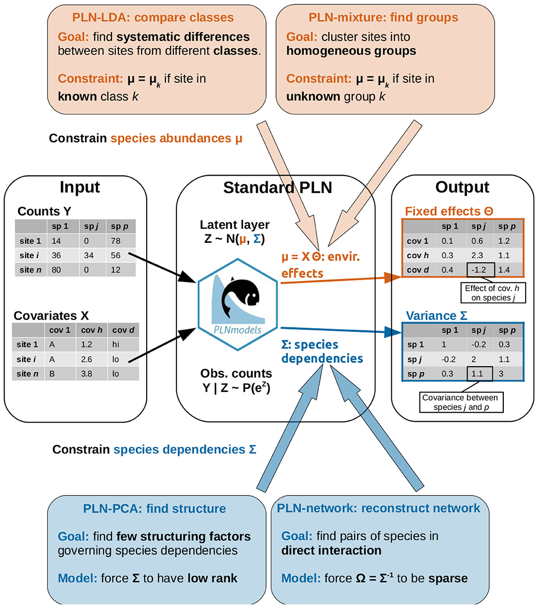
Figure 1. Graphical abstract of the article: the standard PLN model, its extension and the research questions addressed by each method.

1.2. State of the Art

Multivariate count data are increasingly common and a wealth of new methods have been developed in the last decade to analyze them. As stated before, most of them (including the PLN model) fall in the family of latent variable models (LVMs), and more specifically of multivariate generalized linear mixed models (mGLMMs), also called generalized linear latent variable models (GLLVMs) when the mixed effect is degenerate and has small rank. In those models, the distribution of observed responses usually belong to the exponential family (Bernoulli, Binomial, Poisson, Negative-Binomial, with or without Zero-Inflation, etc.) or the exponential dispersion model (Tweedie, etc.). In both cases, model parameters are related to linear combinations of latent variables (and possibly covariates) through a simple link function.

The latent variables can be constrained in various ways to achieve different goals. For example, Warton et al. (2015) uses GLLVM (i.e., GLMM with low-dimensional latent variables) and a Bernoulli observation layer to perform ordination (also called dimension reduction) on presence/absence data. mGLMM naturally accomodate covariates but can be complex to adjust to data. Warton et al. (2015) reviews several estimation technique ranging from fast and potentially inaccurate (Laplace approximation) to accurate but very slow (MCMC used in Hui, 2016; Tikhonov et al., 2020) or even untractable (EM). mGLMM can also be combined with mixture models to perform sample clustering (Hui et al., 2015). Unfortunately, model fitting is once again difficult due to the complexity of the likelihood in those models and requires specific techniques, as detailed in Pledger and Arnold (2014). Variational approximation has proved a very successful inference technique, both fast and accurate, for such complex likelihood models and is now the default for GLLVM (Hui et al., 2017; Niku et al., 2019b).

Hierarchical Modeling of Species Communities (HMSC), introduced in Ovaskainen et al. (2017), is another instance of GLLVM. The main difference with GLLVM as presented in Hui et al. (2017) is that the latent variables in HMSC are themselves carefully modeled according to a hierarchical framework with clearly identified terms and effects (species traits, species phylogeny, etc.) to ease interpretation of the parameters and decompose variance across terms. This is again a model with complex likelihood and parameters are estimated using MCMC techniques (Tikhonov et al., 2020), thus limiting its use to medium-sized problems (a few dozen species in the published examples).

The PLN model introduced here is yet another instance of the rich family of GLLVM which takes the middle road. Our goal is to develop a generic and versatile umbrella framework under which one can perform various tasks: ordination (Chiquet et al., 2018), classification, group prediction, network inference (Chiquet et al., 2019), etc. Unlike Hui et al. (2017), and in line with Ovaskainen et al. (2017), we allow the user to carefully constrain the model parameters: each set of constraints leading to a different task. In contrast to HMSC, we do not specify a grand overarching model but rather several easier to estimate variations around a central model. In addition, we want to analyze large datasets, similarly to Hui et al. (2017), and thus rely on the efficient inference machinery of variational approximation rather the slower MCMC. Finally, and unlike Ovaskainen et al. (2017) and Hui et al. (2017), we only deal with count data (not presence / absence data) and leverage our use of the (Zero-Inflated) Poisson distribution to derive fast and scalable estimation procedures.

1.3. The Poisson-Lognormal Model

The multivariate Poisson-lognormal model (Aitchison and Ho, 1989) is designed for the analysis of an abundance table, that is typically a n × p count matrix Y, where Y_ij is the number of individuals from species j observed in site i, n being the number of sites and p the number of species. Note that site may actually refer to a sample or an experiment, and a species to an Operational Taxonomic Unit (OTU) or an Amplicon Sequence Variant (ASV), both of which are proxies for species frequently used in metabarcoding surveys. Similarly, the number of individuals may correspond to a number of reads in metabarcoding experiments.

The PLN models relates the p-dimensional abundance vector Y_i collected in site i with a p-dimensional Gaussien latent vector Z_i as follows:

$\begin{array}{ll}\begin{array}{c}\text{\hspace{1em}\hspace{1em} latent layer:\hspace{1em}\hspace{1em} }{Z}_i~{N}({\mu }_i,\Sigma )\hfill \\ \text{observation layer: }{Y}_{ij}\mid Z_{ij}~{P}(exp(o_{ij}+Z_{ij}))\end{array}& (1)\end{array}$

where the Z_i are assumed to be independent (across sites) and the abundances Y_ij are all conditionally independent given the latent variables Z_ij. The parameter ${\mu }_i={\left[{\mu }_{ij}\right]}_{1\le j\le p}\in {ℝ}^p$ corresponds to the fixed effects, and is related to the expected log-abundances, whereas the latent covariance matrix Σ = [σ_jk]_1≤j,k≤p describes the underlying structure of dependence between the p species. In this simple form, the PLN model therefore assumes that the dependency structure among species is the same across all sites. All extensions presented in section 2 will be about alternative modeling of the latent layer in Equation (1), corresponding to different assumptions exposed in Figure 1.

When environmental covariates are available, the fixed effect μ_ij in the latent layer may be decomposed as ${\mu }_{ij}=x_i^{⊺}{\theta }_j$ where $x_i\in {ℝ}^d$ is a vector of covariates for sample i (e.g., environmental conditions, location, etc.) and ${\theta }_j\in {ℝ}^d$ is a vector of regression coefficients associated to these d covariates for species j. The vectors of regression coefficients θ_j can then be merged into the d × p matrix Θ. The fixed quantity o_ij is the offset for species j in sample i. In the PLN framework, offsets are used to take into account expected differences in observed counts due to imbalanced sampling efforts, such as known heterogeneities in terms, sequencing depths in metabarcoding surveys, collection protocols, species detectability, etc. For examples, if we spend twice as much time looking for species j in site i′ than in site i and thus expect its count to be twice higher (all other things being equal), we set $o_{i^{\prime }j}=o_{ij}+log(2)$.

Likewise in generalized linear models, the parameters should be interpreted according to the properties of the multivariate Poisson-lognormal distribution. Some remarks can be made about the first and second order moments, which are given by Aitchison and Ho (1989):

$\begin{array}{l}\begin{array}{c}\text{\hspace{1em} \hspace{1em}mean:\hspace{1em}\hspace{1em} }𝔼(Y_{ij})=exp(o_{ij}+{\mu }_{ij}+{\sigma }_{jj}/2)>0,\hfill \\ \text{\hspace{1em}variance:\hspace{1em} \hspace{1em}}𝕍(Y_{ij})=𝔼(Y_{ij})+𝔼{(Y_{ij})}^2(e^{{\sigma }_{jj}}-1)>𝔼(Y_{ij}),\hfill \\ \text{covariance: }ℂ\text{ov}(Y_{ij},Y_{ik})=𝔼(Y_{ij})𝔼(Y_{ik})({𝔼}^{{\sigma }_{jk}}-1).\hfill \end{array}\end{array}$

1. Expected count: Due to the logarithmic link function, the expected abundance 𝔼(Y_ij) of species j in site i is not simply exp(o_ij + μ_ij) as the variance parameter σ_jj is also involved.

2. Over-dispersion: Because of the presence of a latent (random) layer, the PLN model displays a larger variance than the Poisson model for which 𝕍(Y_ij) = 𝔼(Y_ij).

3. Faithful correlation: Because ${𝔼}^{{\sigma }_{jk}}-1$ has the same sign as σ_jk, the covariance (resp. correlation) between the respective abundances Y_ij and Y_ik of species j and k has the same sign as the covariance (resp. correlation) between the corresponding latent components Z_ij and Z_ik.

The last property is especially desirable as it means that the correlation structure of the latent vector Z_i preserves that of the observed abundances Y_i. As a consequence, the independence of Z_ij and Z_ik (σ_jk = 0) induces an absence of correlation between Y_ij and Y_ik (ℂov(Y_ij, Y_ik) = 0).

1.4. A First Example

As a first illustration of the use of the PLN model for analyzing abundance data, we consider the dataset introduced by Fossheim et al. (2006) (and re-analyzed by Greenacre, 2013; Greenacre and Primicerio, 2014), which consists in the abundances of p = 30 fish species measured in n = 89 sites of the Barents sea between April and May 1997. The species under study are sensitive to environmental drivers (temperature, water depth, …) but are also related by trophic interactions. A first aim is to study the relative contribution of each type of interaction (abiotic vs. biotic) to the structure of the community.

Captures were carried out with the same protocol for all species and all sites, so no offset term is required here. For each site i, four covariates were recorded: the latitude, the longitude, the depth and the temperature, which constitute the vector x_i. We also add an intercept to these covariates to capture differences in the base abundances of our 30 species. The covariates can be gathered into a n × (d = 5) matrix X.

Fitting the PLN model (using the algorithm outlined in section 3 and described in detail in Appendix) results in a matrix of regression coefficients $\hat{\Theta }$ and a latent covariance matrix $\hat{\Sigma }$. Figure 2 shows these estimates. The most contrasted regression coefficient turns out to be the intercept, revealing a great variability between the mean abundances of the species, not well-explained by covariates. The latent correlation structure encoded in $\hat{\Sigma }$ reveals some subgroups of species: the covariation between these species are not caused by the effects of the recorded covariates and may reflect high order structure.

FIGURE 2

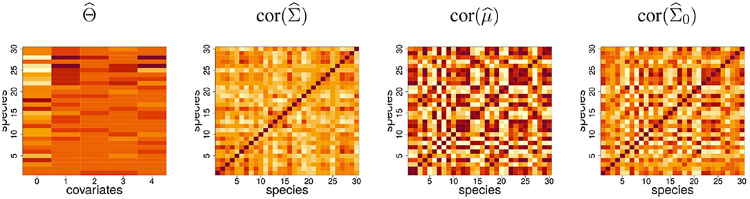
Figure 2. Fit of the PLN model to the Barents fish data set. $\hat{\Theta }=$ intercept (labeled 0) and regression coefficients for the four covariates and the 30 species; $\mathrm{\text{cor}}(\hat{\Sigma }),$ estimated latent correlation matrix; $\mathrm{\text{cor}}(\hat{\mu }),$ correlation matrix of the predicted log-abundances; $\mathrm{\text{cor}}({\hat{\Sigma }}_0),$ estimated correlation matrix for the null model, which includes only an intercept term.

Based on this, a predicted log-abundance can be computed for each species at each site as ${\hat{\mu }}_{ij}=x_i^{⊺}{\hat{\theta }}_j+{\hat{\sigma }}_{jj}/2$. Interestingly the correlation structure between these predicted log-abundances is very contrasted compared to $\hat{\Sigma }$. This shows that a substantial part of the covariation between species abundances is driven by the covariates. To illustrate this point, we fitted a model with only an intercept term, yielding the null covariance matrix ${\hat{\Sigma }}_0$, which captures the covariation between species due to both biotic and abiotic effects. We observe that ${\hat{\Sigma }}_0$ displays a structure quite similar to the correlation matrix of the prediction $\hat{\mu }$, which shows the predominant contribution of environmental effects to empirical covariations.

2. Adapting the PLN Framework to Different Tasks

We now introduce a series of extensions of the basic PLN model defined in Equation (1). As explained above, the PLN model deals with both abiotic effects through the mean vector μ_i and biotic effects by describing species interactions through the variance matrix Σ. As shown in Figure 1, the first two extensions (LDA and clustering) deal with the former and typically aim at analyzing abiotic (or environmental) effects. The last two extensions (PCA and network inference) are about the latter and provide insights about the dependency structure between the species.

Each method will be accompanied with a specific example. LDA will be used to compare the bacterial communities collected in different body sites of dairy cattle. Model-based clustering will be applied to the microbiota of leaves from several oaks and will prove to be able to recover, in a blind way, the tree of origin of each leaf. Dimension reduction using PCA will be applied to the same dataset for visualization purposes and to exhibit which species contribute most to the community structure. The last example is an attempt to reconstruct the interaction network of fish species from the Barents Sea.

2.1. Sample Comparison With Linear Discriminant Analysis

A first variant of the PLN model is the analog of the Linear Discriminant Analysis (LDA) to Poisson-lognormal models. It applies to labeled data, i.e., when sites belong to known classes (e.g., anatomical sites for host-associated microbiota, or geographical areas in ecogeography) and the objective is two-fold: identify class-based differences in species counts and predict the class of an unlabeled site based on its species counts. As valuable byproducts, classification accuracy assesses whether the classes are really different and species with a high contribution to the discriminant axes can serve as biomarkers.

2.1.1. The PLN-LDA Model

Informally, PLN-LDA assumes that (i) the sites belong to distinct and known classes, (ii) all sites in the same class have the same mean species abundances, and (iii) those mean abundances may differ between classes but (iv) species interact in the same way in all classes. Formally, PLN-LDA for multivariate count data is a PLN model with an additional class covariate and a different decomposition of the mean vectors μ_i. Assume the classes are labeled by k ∈ {1, …, K} and denote by k_i ∈ {1, …, K} the known class of site i. Finally, denote by ${\overline{\mu }}_k$ the mean vector in class k. The PLN-LDA model is the same as (1), where

$\begin{array}{ll}\text{latent layer: }{Z}_i~{N}({\overline{\mu }}_k,\Sigma )\text{if site }i\text{ belongs to class }k\text{: }{k}_i=k.& (2)\end{array}$

Compared to the standard PLN model (1), we need to estimate the additional class mean vectors $\left\{{\overline{\mu }}_k,k=1,\dots ,K\right\}$. In presence of covariates, Model (2) can be extended to $Z_i~{N}(x_i^{⊺}\Theta +{\overline{\mu }}_k,\Sigma )$.

Discriminant Axes and Prediction

Once estimated, the class means $\left\{{\overline{\mu }}_1,\dots ,{\overline{\mu }}_K\right\}$ and reconstructed latent means M can be used to find axes of maximal discrimination of the classes in the latent layer, likewise in standard LDA. Scores along those axes can be used for visualization purposes and contributions of species to each axis can be used to identify systematic differences in abundances between the classes and potential biomarkers.

The classification of a new site from its species counts Y_new is based on Bayes' rule. We first estimate the variational likelihood $f_k(Y_{\mathrm{\text{new}}})={J}(Y_{\mathrm{\text{new}}};{\hat{\overline{\mu }}}_k,\hat{\Sigma },M_{\mathrm{\text{new}}},S_{\mathrm{\text{new}}})$ of observing counts Y_new if the new site was in class k. Note that ${\hat{\overline{\mu }}}_k$ and $\hat{\Sigma }$ are extracted from the PLN-LDA fitted on the training sites whereas the variational parameters M_new and S_new must be optimized with respect to Y_new. This corresponds to the VE step mentioned in section 3. We then use an estimator ${\hat{\pi }}_k$ of the proportion of class k (typically the proportion of sites of class k among the learning sites). The posterior probability for the new site to belong to class k is then estimated by

$\begin{array}{ll}{\tau }_{\text{new},k}={\hat{\pi }}_k{f}_k(Y_{\text{new}})/\left({\displaystyle \sum _{\ell =1}^K}{\hat{\pi }}_{\ell }{f}_{\ell }(Y_{\text{new}})\right).& (3)\end{array}$

2.1.2. Cow Holobionts

To illustrate PLN-LDA, we consider the dataset introduced in Mariadassou et al. (2020) which consists of n = 256 bacterial communities sampled on three body sites (nose, mouth, and vagina) of 45 primiparous Prim'Holstein dairy cattle. The cattle comes from two divergent lineages, each sampled twice (1 month and 3 months after first delivery). Communities were sequenced using the hypervariable V3-V4 region of 16S rRNA as marker-gene. Sequences were cleaned and analyzed with DADA2 (Callahan et al., 2016) to create p = 1, 077 Amplicon Sequence Variants (ASVs). The aim is to assess whether the communities living in different body sites are different and how they differ.

We analyzed this data set by running PLN-LDA with time and lineage as covariates and body site as class. Offsets were computed as the log-total sums of counts over the 1,077 ASVs, but we kept only 53 ubiquitous ASVs (with prevalence higher than 20% in at least one class) for the discriminant analysis. The 256 communities were split in two halves: a training test used to estimate the parameters and a test set used to assess the classification accuracy.

The results of our analysis with PLN-LDA are displayed in Figure 3A shows that the first discriminant axis (LDA 1) separates vagina from nose and mouth whereas the LDA 2 separates nose from mouth. The inset correlation map shows the contribution of ASVs to LDAs: some ASVs are shared between nose and mouth or nose and vagina but almost none is shared between mouth and vagina. This is also obvious in the count matrix featured in Figure 3B where ASVs are reordered according to their position in the correlation map. The block structure indicates a strong association between some groups of species and body sites. Figures 3C,D show the same views for test samples. The inset confusion table of Figure 3C shows a prediction accuracy of 95% (7 misclassified samples out of 128). The count matrices allow us to focus on the misclassified samples. Three out of the 5 misclassified vagina samples have very small counts for all species. For those samples, the posterior probability of the second best class is around 0.25, indicating a quite high uncertainty. The misclassified nose (resp. mouth) sample is depleted in ubiquitous species typically found in other nose (resp. mouth) samples.

FIGURE 3

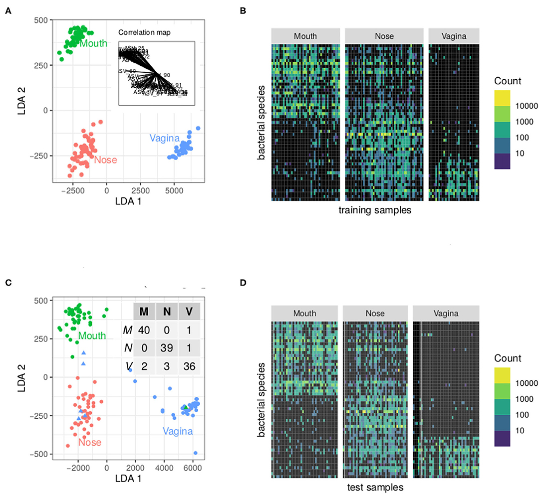
Figure 3. Result of the analysis of the cow holobionts data set with PLN-LDA: a few ASV are enough to find accurately discriminate the body sites. (A) Scores of the training communities on the discriminant axes and contribution of the ASV to each axis (inset graph). (B) Matrix of reordered counts (log-scales). ASV are ordered according to their angle with the x-axis in the correlation map. (C) Scores of the test communities and confusion matrix of the classification (inset table). Misclassified communities are shown by triangles. (D) Matrix of counts as in (B). Misclassified communities are located on the left of their respective panels and separated from the rest by a gray line.

2.2. Unsupervised Classification With Model-Based Clustering

This second variant is the analog of Gaussian mixture models for Poisson-lognormal models. The objective is to perform model-based clustering on multivariate count tables, in order to find groups of homogeneous sites or samples in the data set.

2.2.1. The PLN-Mixture Model

Informally, PLN-mixtures assumes that (i) the sites belong to K unknown groups, with different frequencies, (ii) all sites in the same group are homogeneous: they have the same mean species abundances and species interact in the same way in all sites, (iii) those mean abundances and interactions may differ between groups. Formally, PLN-mixture for multivariate count data is a PLN model with two latent layers: the first layer describes the (unknown) group membership of each site and the second layer embeds the distribution of the hidden site's multivariate Gaussian vector conditional on its group membership. Note K the number of groups and C_i ∈ {1, …, K} the (unknown) group of site i. The PLN-mixture model assumes that each site has a probability π_k to belong to group k, so that C_i has a multinomial distribution. The latent vector Z_i associated with a site from group k is then assumed to have a multivariate Gaussian distribution with group-specific parameters ${N}({\overline{\mu }}_k,{\Sigma }_k)$. The latent layer of the original model (1) is therefore split as follows:

$\begin{array}{ll}\begin{array}{c}\text{latent layer 1:\hspace{1em}\hspace{1em}\hspace{1em}\hspace{1em}}{C}_i~{M}(1,\pi =({\pi }_1,\dots ,{\pi }_K)),\hfill \\ \text{latent layer 2: }{Z}_i\mid C_i=k~{N}({\overline{\mu }}_k,{\Sigma }_k),\hfill \end{array}& (4)\end{array}$

where the ${\overline{\mu }}_k$'s and Σ_k's are the respective vector of means and the covariance matrix of the K components of the mixture, and π is the vector of the mixture proportions. Compared to the standard PLN model (1), we need to estimate the parameters $\left\{{\overline{\mu }}_k,{\Sigma }_k,{\pi }_k,k=1,\dots ,K\right\}$ as well as the group membership – or cluster – C_i of each sample. Covariates can also be included in the PLN-mixture model, changing the second layer of Equation (4) into $(Z_i\mid C_i=k)~{N}({\overline{\mu }}_k+x_i^{⊺}\Theta ,{\Sigma }_k)$. This extension is useful to correct for known environmental structuring factors and recover some residual group structure among the sites. Note that the model differs from previous works: (Pledger and Arnold, 2014) considers a discrete group structure but accounts for neither latent variables nor covariates and Hui et al. (2015) accounts for covariates and latent variables but not a discrete group structure, as it is designed for ordination rather than clustering. PLN-mixture is the only one to account for covariates, a latent structure and a cluster structure, all at the same time.

The main difference between the PLN-LDA and PLN-mixture models is that the group (or class) memberships of the sites are known in the former, whereas they need to be inferred in the latter. The other difference is that the current implementation of PLN-mixture allows the covariance matrix Σ to vary across groups, whereas it is assumed to be constant in PLN-LDA. An important byproduct of the PLN-mixture model is the posterior probability, which can be used to actually classify sites into groups. These probabilities are iteratively computed in the algorithm using Equation (3).

Parametrization of the Covariance in PLN-Mixture Models

When using parametric mixture models like Gaussian mixture models, it is not recommended to consider general covariance matrices Σ_k with no special restriction, especially when dealing with a large number of species. Indeed, the total number of parameters to estimate in the model can become prohibitive: in the general case, a PLN-mixture model with K components like in (4) has K × (p + p(p + 1)/2) model parameters, plus the K × 2(n × p) variational parameters. To reduce the computational burden and avoid over-fitting two different, more constrained parameterizations of the covariance matrices of each component are currently implemented in the PLNmodels package (on top of the general form of Σ_k):

$\begin{array}{l}\begin{array}{c}\text{ diagonal covariances:}{\Sigma }_k=diag(d_k)\text{ (}2Kp\text{ parameters),}\hfill \\ \text{spherical covariances:}{\Sigma }_k={\sigma }_k^{2}I\text{\hspace{1em}\hspace{1em}\hspace{1em}(}K(p+1)\text{ parameters).}\hfill \end{array}\end{array}$

The diagonal structure assumes that, given the group membership of a site, all species abundances are independent. The spherical structure further assumes that all species have the same biological variability. In particular, in both parametrization, all observed covariations are caused only by the group structure. For readers familiar with the mclustR package (Fraley and Raftery, 1999), which implements Gaussian mixture models with many variants of covariance matrices of each component, the spherical model corresponds to VII (spherical, unequal volume) and the diagonal model to VVI (diagonal, varying volume and shape). Using constrained forms of the covariance matrices enables PLN-mixture to provide a clustering even when the number of sites n remains of the same order, or smaller, than the number of species p.

2.2.2. Oaks Powdery Mildew

To illustrate PLN-mixture, we consider the dataset introduced in Jakuschkin et al. (2016) which consists of microbial communities sampled on the surface of n = 116 oak leaves. Communities were sequenced with both the hypervariable V6 region of 16S rRNA as marker-gene for bacteria and the ITS1 as marker-gene for fungi. Sequences were cleaned, clustered at the 97% identity level to create OTUs and only the most abundant ones were kept (see Jakuschkin et al., 2016 for details) resulting in a total of p = 114 OTUs (66 bacterial ones and 48 fungal ones). One aim of this experiment is to understand the association between the abundance of the fungal pathogenic species E. alphitoides, responsible for the oak powdery mildew, and the other species. Furthermore, the leaves were collected on three trees with different resistance levels to the pathogen, which we call the tree susceptibility. We use this example to assess the ability of model-based clustering to recover, without feeding this information to the model, the existence of groups of leaves with different origins.

We analyzed this data set by running PLN-mixture for a number of component varying from 1 to 6. We selected the final number of components with a variant of the Integrated Classification Likelihood (ICL: Biernacki et al., 2000), tuned for our own PLN framework. Since the abundances were measured separately for fungi and bacteria, we define a different offset term o_ij for each OTU type to take into account the differences in sampling effort and marker genes. Offsets are still computed as the log-total sums of reads, including those of filtered out OTUs, for each OTU type.

The results of our analysis with PLN-mixture are displayed in Figure 4A shows the evolution of the approximated log-likelihood (which is strictly increasing with the number of components, as expected) and the evolution of the ICL criterion, which suggest a model with 4 or 5 components. Figure 4B displays a scatter-plot of the expected latent position ${\hat{Z}}_i$, after performing simple PCA since pairs-to-pairs plot would be unreadable with p = 114 species. We also colored the site according to the most probable components according to our PLN-mixture, which shows that we recover the strong latent structure visible in the individual factor map. On Figure 4C, we compare the memberships of the series of PLN-mixture model with the tree susceptibility, by means of various measures for clustering comparison (ARI, AMI, and NID, see Vinh et al., 2010). It then becomes obvious that the clustering found by PLN-mixture is highly related to the susceptibility level of each tree. Note that, even if apparently quite strong, this pattern in the data is not directly visible on the table of counts, as shown by the re-ordered version of the expected counts, shown in Figure 4D. This somewhat supports the modeling strategy of PLN-mixture and PLN in general, with a Poisson emission and a latent Gaussian layer.

FIGURE 4

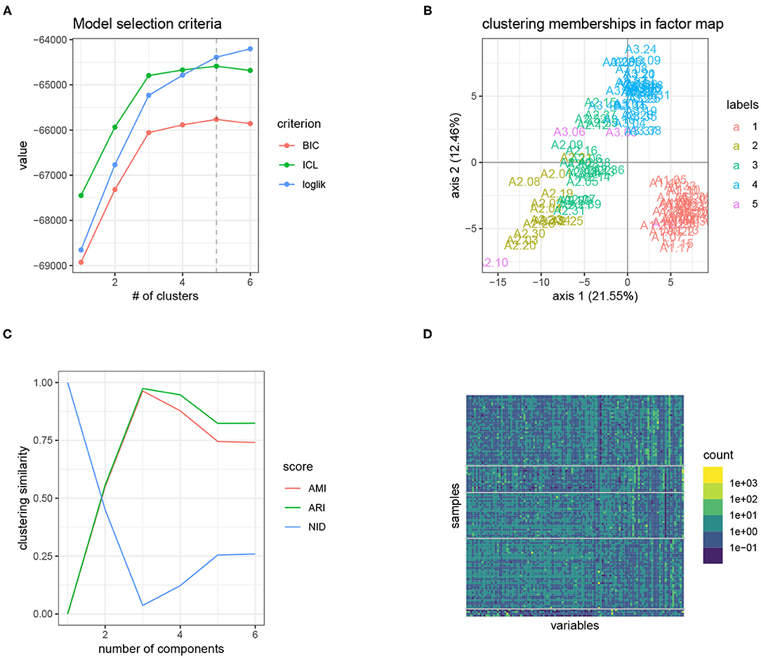
Figure 4. Result of the analysis of the oaks powdery mildew data set with PLN-mixture: the tree susceptibility to the pathogen is easily recovered, and seems to strongly structure the data set. (A) Model selection criteria used to select the number of component: (ICL chooses 5 clusters). (B) Scatter-plot after dimension reduction, with samples colored according to the clustering found. (C) Similarity between the inferred clustering and tree susceptibility with standard comparison measures. A high similarity yields in high AMI and ARI, but low NID. (D) Matrix of counts re-ordered (log-scale): the blocks share much with the level of susceptibility. The first two blocks the more heterogenous group of susceptible trees.

2.3. Dimension Reduction With Principal Component Analysis

We now turn to the extensions of the PLN model (1) that mostly deal with the modeling of the dependency between species, which is encoded in the covariance matrix Σ. One first way to depict species dependency is to look for a few underlying (that is: unknown) factors that may have an impact on the whole community. The intuition behind this reasoning is that the p species actually respond to few unobserved drivers that structure most of their variations. As a consequence, finding such factors amounts to performing dimension reduction, as it suggests that the variations of abundances can be summarized in a virtual space with much fewer dimensions than the number of species. This is especially desirable for studies involving a large number of species, when one looks for important patterns of diversity and tries to find structure in large data sets. This is exactly what principal component analysis (PCA) is designed for, especially in its probabilistic PCA variant, which can be easily extended to count data using the PLN framework. We illustrate the PLN-PCA model by continuing the analysis started in the previous section on the oaks powdery mildew data set.

2.3.1. Probabilistic Poisson PCA With PLN Model

In the standard PLN model (1), the latent vector Z belongs to a latent space of dimension p, with one dimension per species. This assumes that any species can co-vary arbitrarily with any other, which allows for fine scale inferences but also becomes costly very quickly when the number of species p increases. PLN-PCA assumes instead the existence of q (with q ≪ p) strong structuring unknown factors (e.g., environmental filters) that govern the fluctuations of all species. All observed covariations between species then reflect those factors. Formally, PLN-PCA assumes that the latent vectors Z_i are fully determined by q structuring factors as follows:

$\begin{array}{l}\begin{array}{c}\text{\hspace{1em}\hspace{1em}scores:\hspace{1em}}{W}_i~{N}(0_q,I_q)\hfill \\ \text{latent layer:\hspace{1em}}{Z}_i=B^{\top }{W}_i\hfill \end{array}\end{array}$

where the W_i's are supposed to be iid. As a consequence, the Z_i's are iid as well, with distribution

$\begin{array}{ll}{Z}_i~{N}(\mu ,\Sigma =B{B}^{\top }).& (5)\end{array}$

This is a strict extension of the probabilistic PCA model of Tipping and Bishop (1999) to the PLN model which we detail in Chiquet et al. (2018). Similar models can be found in the literature, like the Poisson variant of the GLLVM family detailed in Warton et al. (2015) and Niku et al. (2017). One advantage of PLN-PCA is to be part of the unifying PLN framework. The p × q matrix B is the analog of the rescaled loadings in PCA: B_jh measures the impact of the h-th factor on the j-th species. Likewise, W_i is a score vector: W_ih is the value of the h-th factor for the i-th observation. The dimension q corresponds to the number of structuring factors, or equivalently to the number of axes in the PCA and the rank of Σ = BB^⊤. The PLN-PCA model can thus be viewed as a PLN model with the low rank constraint rank(Σ) = q on the covariance matrix Σ. The number of parameters in the PLN-PCA model is (p + 1)q, down from p(p + 1)/2 in the standard model. Again, we can simply include covariates in the PLN-PCA model by changing Equation (5) into $Z_i~{N}(x_i^{⊺}\Theta ,B{B}^{\top })$. This is useful to correct for strong known structuring factors and to investigate weaker factors.

2.3.2. Oaks Powdery Mildew

We continue the analysis of the oaks data set begun for PLN-mixture. As seen before, there is an obvious structure in the data explained by the tree susceptibility. Knowing this, one may be interested in exhibiting a remaining dependence structure that is not induced by the tree susceptibility.

In Figure 5A, we represent the biplot for the first two principle components obtained with PLN-PCA, not accounting for the tree susceptibility, after selecting the best possible rank q thank to the ICL criterion. As expected after our clustering study with PLN-mixture, the factorial map exhibits a strong structure where individuals are spread into three groups corresponding to the level of susceptibility of the trees where the leaves were sampled. We also projected the 10 species with the highest contribution to the first two principal components. Interestingly, the pathogen E. alphitoides point toward the group of susceptible trees, indicating that the presence of the disease is one of the main underlying drivers.

FIGURE 5

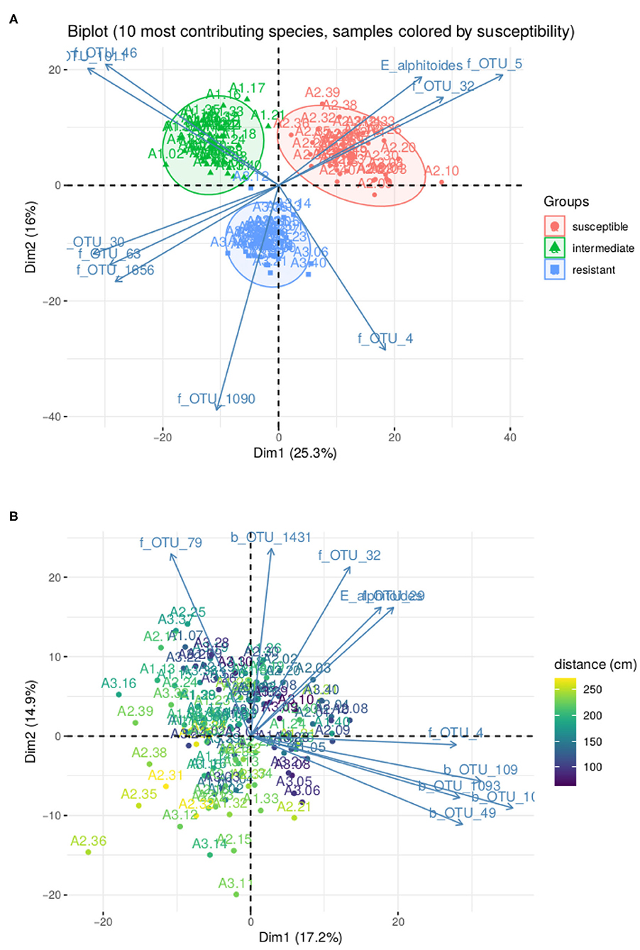
Figure 5. Result of PLN-PCA analysis on oaks powdery mildew data set. (A) Biplot for the first two axes without correction for susceptibility. (B) Biplot for the first two axes after correction for susceptibility. Color gradient corresponds to distance to ground.

In Figure 5B, we show how PLN-PCA can help exploring second-order structuring effects that are masked by strong first-order effect, that is here: the tree susceptibility. To do so, we included the susceptibility as a covariate to remove its effect and highlight a weaker effect: the map shows that the communities are structured by the distance of the leaf to the ground. The effect of covariates on the abundance of E. alphitoides were also consistent. When taking the susceptible tree as a reference, the estimated parameters θ_ij associated with the intermediate and resistant trees were respectively −3.94 (~ 50-fold abundance decrease) and −7.05 (~ 1,000-fold abundance decrease).

2.4. Network Inference

As a last extension of the PLN model, we introduce the analog of graphical-Lasso (Banerjee et al., 2008; Friedman et al., 2008) for the inference of interaction networks. The ultimate goal is to find pairs of species that are genuinely interacting, for example through trophic relationships. Those genuine, direct, interactions are hard to identify from covariation patterns in general as many different mechanisms can lead to the same patterns. For example, shared habitat preferences or reliance for growth on a metabolite produced by a third species, none of which requires direct interaction, (see e.g., Popovic et al., 2019), can lead to statistical associations that are indistinguishable from those of obligate symbiosis, an extreme form of interaction.

Formally, species can be associated but they are in direct interaction only if they are still dependent after conditioning on both the covariates (abiotic effects) and all the other species (biotic effects). In the Gaussian setting, this distinction coincides with the difference between correlation and partial correlation. Correlations between pairs of species is captured by the variance matrix Σ, whereas partial correlations are encoded by its inverse: the precision matrix $\Omega ={\left[{\omega }_{jk}\right]}_{1\le j,k\le p}={\Sigma }^{-1}$. In this setting, species j and k are associated as soon as σ_jk ≠ 0 but are in direct interaction if and only if ω_jk ≠ 0 (Lauritzen, 1996).

2.4.1. Network Inference With the PLN Model

The PLN network model for multivariate count data can be viewed as a PLN model with a constraint on the coefficients of Ω. Because the network is usually supposed to be sparse (i.e., only a few pairs of species are expected to be in direct interaction), we assume that the precision matrix Ω is sparse and the PLN-network model is the same as (1) with

$\begin{array}{ll}\text{latent layer}:Z_i~{N}(m_i,{\Omega }^{-1})\text{with}\Omega \text{ sparse}.& (6)\end{array}$

Both the PLN-PCA and the PLN-network models impose constraints on the covariance matrix Σ, but the low-rank constraint used in PLN-PCA aims at identifying few important unknown structuring factors, whereas the sparsity constraint used in PLN-Network aims at identifying direct interactions between species. Unlike previous extensions, this requires substantial modification of the objective function to be optimized, which becomes:

${J}(Y;\Theta ,{\Omega }^{-1},M,S)+\lambda |\Omega {|}_{1,0}$

where |Ω|_1,0 is the sum of the absolute values of the non-diagonal terms of Ω (diagonal terms are not penalized) and λ is a penalty coefficient. The term λ|Ω|_1,0 forces many coefficients of $\hat{\Omega }$ to be null. This is an extension of the graphical-Lasso (Banerjee et al., 2008; Friedman et al., 2008) to the PLN model (Chiquet et al., 2019). The parameter λ controls the number of edges in the network (larger λ yields fewer edges) and can be chosen in various ways, including model selection (Foygel and Drton, 2010) and resampling (Liu et al., 2010).

2.4.2. Barents Fish

We illustrate the use of the PLN-network model on the Barents fish dataset. We focus on the way the inferred network is modified when introducing covariates in the model. To this aim, we fitted the PLN-network model with (a) no covariates, (b) two environmental covariates (temperature and depth), and (c) all covariates (i.e., the previous two plus the geographical location) using a common λ-grid (with 20 values spaced equally in log scale between λ_min = 0.03 to λ_max = 15.17) for al models.

Figure 6 (top right panel) shows that the number of edges increases as the penalty decreases, as expected. It also shows that, for any penalty, the number of edges decreases as (plain lines) the richness of the number of edges increases (c > b > a) and that most edges recovered in the full (c) model are also recovered in the partial models (a, black dotted curve) and (b, blue dotted curve). This suggests that naive inference identifies not only genuine edges but also spurious ones corresponding to co-variations induced shared habitat preferences (captured here by temperature, depth, and location). Interestingly, the dotted curve shows that the proportion of common edges between models b and c is higher than the one between models a and c. This suggests that environmental covariates rather than geographical location explain a substantial part of the apparent species co-variations.

FIGURE 6

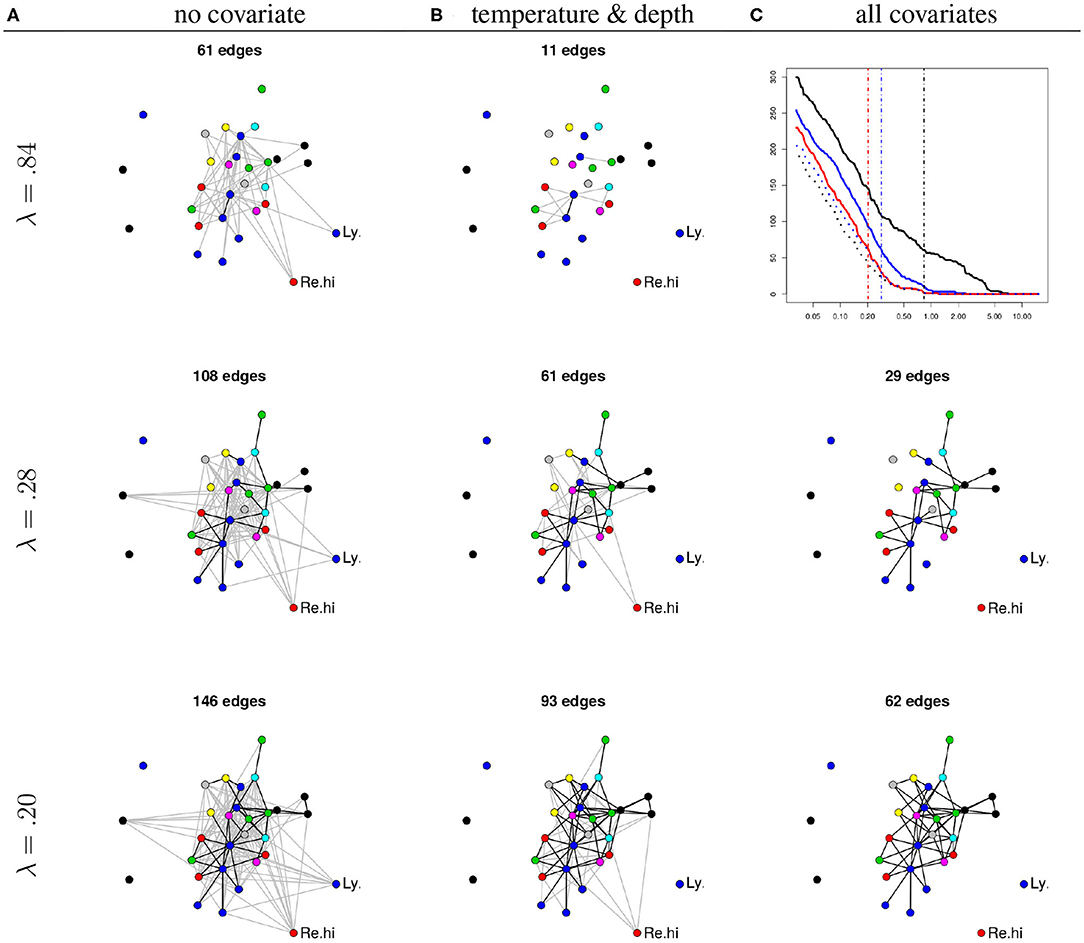
Figure 6. (A) Networks inferred under the null model (no covariates). (B) Networks inferred using temperature and depth as covariates. (C) Networks inferred using all available covariates. All networks are inferred under increasing penalties (top: λ = 0.84, middle: λ = 0.28, bottom: λ = 0.20). Each node corresponds to a given species. The position of the nodes are kept fixed. Node color: species family (see Fossheim et al., 2006). Black edges: edges in common with the network inferred with all covariates and same λ. The missing network (top right panel, all covariates and λ = 0.84) contains only one edge. Top right: number of edges as a function of λ. Black: no covariate, blue: temperature and depth, red: all covariates, dotted black: common edges with no and all covariates, dotted blue: common edges between two and all covariates. Vertical dashed lines: the three chosen values of λ.

The rest of Figure 6 displays the networks inferred with the three models for three different levels of sparsity (controlled by λ). For an illustrative purpose, the values of λ have been chosen so that, in average, each species interacts with two others for each of the three models (a), (b), and (c). This results in networks with approximately 2p = 60 edges. One conclusion is that a set of core species seem to have direct interactions, or at least, interactions that cannot be simply explained by geographical location and environmental covariates (bottom right panel).

On the contrary, some interactions seem to be actually indirect. For example, the interactions between the longear eelpout (Ly.se) and some species from the core group disappear when accounting for temperature and depth, suggesting that the covariation of their respective abundances results from shared environmental preferences. Similarly, the interactions between the Greenland halibut (Re.hi) and the core group is kept when correcting for temperature and depths, but disappears when correcting for location (longitude and latitude) suggesting that these interactions actually reflect a common response to fluctuations of biotic or abiotic characteristics across sites. To confirm this interpretation, we fitted an over-dispersed Poisson generalized linear model for the abundance of both species (not shown). We found that both temperature and depth have a significant effect on the abundance of the longear eelpout and that the longitude has a significant influence on the abundance of the Greenland halibut (all corresponding p-values being smaller than 10⁻⁴).

3. Parameter Estimation

3.1. Variational Inference Algorithm

A specific inference algorithm obviously needs to be designed for each version of the PLN model described in section 2. We do not provide a detailed description for each of them. We rather introduce the general framework of variational inference, which is common to all of them, using the simple PLN model defined in Equation (1) and illustrated in section 1.4 as an example.

Because the latent layer Z is not observed, the PLN model is an incomplete data model in the sense of Dempster et al. (1977), who introduced the celebrated EM algorithm to perform maximum likelihood for such models. This is an iterative, two-steps algorithm. Intuitively, the E step retrieves, from the observed counts Y_i, all the information about the latent vectors Z_i's that is needed, during the M step, to estimate the parameters Θ and Σ. More formally, the E step requires the evaluation of the conditional distribution of the latent vectors given the observed counts, that is: p(Z ∣ Y). Unfortunately, this distribution is intractable for the PLN model, so we resort to a variational approximation (see e.g., Jaakkola, 2001) of this conditional distribution. This results in what is called a variational EM (VEM) algorithm, which alternates the following two steps until convergence:

1. VE step: Given the current estimates $\hat{\Theta }$ and $\hat{\Sigma }$ of the parameters, for each site i, find the normal distribution ${N}(m_i,S_i)$ that best fits the (unknown) conditional distribution p(Z_i ∣ Y_i) in terms of Küllback-Leibler (KL) divergence;

2. M step: Given the approximate conditional distribution of the latent Z_i's, update the parameter estimates $\hat{\Theta }$ and $\hat{\Sigma }$.

The approximation precisely lies in the fact that the true conditional distribution p(Z_i ∣ Y_i) is not Gaussian. Hence, the approximate distribution q(Z) is a product over the sites of Gaussian distributions ${N}(Z_i;m_i,S_i)$. The approximate mean m_i and the (diagonal) covariance matrix S_i are called the variational parameters. They can be merged into two n × p matrices, denoted M and S, respectively. Using such an approximation amounts to maximizing a lower bound of the log-likelihood of the data log p(Y; Θ, Σ) (Blei et al., 2017):

$\begin{array}{l}{J}(Y;\Theta ,\Sigma ,M,S)=logp(Y;\Theta ,\Sigma )-KL\hfill \\ \left[q(Z;M,S)\left|\right|p(Z\mid Y;\Theta ,\Sigma )\right].\hfill & (7)\end{array}$

The objective function of the VEM therefore depends on the data Y and has to be optimized with respect to both the model parameters (Θ, Σ: M step) and the variational parameters (M, S: VE step).

We provide the update formulas for the simple PLN model introduced in section 1 in Appendix. An important feature is that these updates either rely on closed-form expressions or consist of convex optimization problems. This latter property guarantees that a unique optimal update exists and that it can be obtained in a computationally efficient manner (using e.g., gradient descent).

We do not provide the update formulas for each of the PLN models introduced in section 2. PLN-LDA and PLN-mixture can be recast as simple variants of the original PLN model and we can thus rely on the same inference algorithm, with a few minor modifications. In contrast, the inference algorithms of PLN-PCA and PLN-network models are quite more involved and detailed respectively in Chiquet et al. (2018) and Chiquet et al. (2019).

Variational approximations have been shown to be computationally efficient for many latent variable models used in many fields (Blei et al., 2017) and many papers have demonstrated the (empirical) accuracy of the resulting estimates based on simulation studies (see e.g., Ormerod and Wand, 2012; Hui et al., 2017; Niku et al., 2019a, for models related to PLN and community ecology). Unfortunately, the general theory about the statistical properties of variational estimates (e.g., consistency, asymptotic normality) is still very scarce and model dependent. For example, Hall et al. (2011) obtained such results for a Poisson mixed model, with replicates but their asymptotic framework does not include the general PLN model we consider.

To summarize: variational inference is useful to estimate parameters in the PLN model as it allows us to bypass the intractable likelihood but this convenience comes at a cost as there are no out of the box theoretical guarantees on the quality of the estimates.

3.2. Parameter Uncertainty

In absence of a general theory for variational estimation in the PLN model, we use large scale simulations to study the empirical properties of the variational estimates of the PLN model.

3.2.1. Simulation Settings

We simulated count data according to a PLN model with the following parameters: number of samples n ∈ {50, 100, 500, 1000, 10000}, number of species p ∈ {20, 200}, number of covariates d ∈ {2, 5, 10}, sampling effort N ∈ {low, medium, high} (calibrated to roughly correspond to total sums of counts per sample of 10⁴, 10⁵, and 10⁶), and noise level σ² ∈ {0.2, 0.5, 1, 2}. These parameters cover values typically observed in real datasets and range from very hard (n = 50, p = 200, d = 10, N = low) to ridiculously easy (n = 10, 000, p = 20, d = 2, N = high).

For each of the 360 parameter combinations, hereafter referred to as simulation setup, we generated a variance matrix Σ as ${\sigma }_{jk}={\sigma }^2{\rho }^{|j-k|}$, with ρ = 0.2, a design matrix X with 1s in the first column (intercept) and all other entries sampled from a standard Gaussian distribution (we also centered all columns but the first one to avoid interplay between the intercept and the covariates), a regression coefficient matrix Θ with all entries sampled from a centered Gaussian distribution with variance 1/d. Those choices ensures (i) a moderate correlation of the counts across species and (ii) the same order of magnitude for the fixed effects (XΘ) and the biological variability of the species (σ²). The normality assumption for entries of X may not perfectly reflect design matrix from real studies but avoids making arbitrary choices for each individual covariates and is usual for such simulation studies.

For each simulation setup, we generated R = 100 count matrices (Y⁽¹⁾, …, Y^(R)), resulting in a total of 36 000 data sets. A PLN model was then fitted to each of those, resulting in R estimates $({\hat{\Theta }}^{(1)},\dots ,{\hat{\Theta }}^{(R)})$ for each original matrix Θ.

3.2.2. Bias

For each simulation setup and each coefficient θ_jh of that setup (were j refers to the species and h to the covariate, including the intercept), we computed the empirical bias as $R^{-1}\sum _{r=1}^R\left({\hat{\theta }}_{jh}^{(r)}-{\theta }_{jh}\right)$ and the Root Mean Squared Error (RMSE) as $\sqrt{R^{-1}\sum _{r=1}^R{\left({\hat{\theta }}_{jh}^{(r)}-{\theta }_{jh}\right)}^2}$. The distribution of those metric are represented in Figure 7A represents boxplots of the bias (one boxplot per setup, computed over all entries of Θ). It shows that the variational estimates are unbiased and, as expected, that the empirical bias decreases when the number of samples (n) increases and when the variability (σ²) decreases (note the different y-axis scales for different values of σ²). Figure 7B likewise shows that the RMSE decreases with increasing n (as $1/\sqrt{n}$) and decreasing values of σ² (note again the different y-axis scales). By contrast, the sampling effort has no effect on the accuracy of the estimates. Considering that the typical scale for coefficient θ_jh is $1/\sqrt{d}$, the RMSE is quite small (below 0.05) as soon as n ≥ 500 sites, for all values of σ² and even as soon as n ≥ 100 for smaller σ².

FIGURE 7

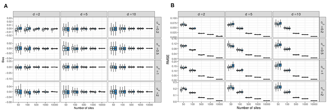
Figure 7. Result of the simulations: variational estimates are unbiased and have low RMSE starting at n = 500 (and even n = 100 for low levels of variability). (A) Empirical bias of the variational estimates ${\hat{\theta }}_{jh}$ (computed over R = 100 replicates, one boxplot per simulation setup). Color codes for sampling effort (lighter to darker: lower to higher). (B) Empirical RMSE of the variational estimates ${\hat{\theta }}_{jh}$ (computed over R = 100 replicates, one boxplot per simulation setup). Color codes for sampling effort (lighter to darker: lower to higher).

3.2.3. Confidence Intervals

Few general theoretical results exist about the statistical properties of variational estimates, but naive approaches are known to provide too narrow confidence intervals (see, e.g., Wang and Titterington, 2005; Westling and McCormick, 2019). One naive approach consists in computing the Fisher information matrix (and deduce the confidence intervals) of the model parameters $\hat{\Theta }$ and $\hat{\Sigma }$ from the variational lower bound of Equation (7), i.e., as if it were the true log-likelihood and not an approximation.

We used our simulation results to study the accuracy of confidence intervals computed this way. More specifically, we computed a 95% confidence interval $I{C}_{95}({\hat{\theta }}_{jh}^{(r)})$ based on the pseudo-Fisher information matrix for each replicate r and computed their empirical coverage, that is the proportion of replicates for which the true parameter θ_jh lies within $I{C}_{95}({\hat{\theta }}_{jh}^{(r)})$. If the confidence intervals are well-calibrated, this proportion should be around 0.95.

The results (not shown here) paint a striking picture as the coverage barely reaches 0.3 for low variability setups (σ² = 0.2) and falls below 0.1 in more difficult setups, especially when the variability is large. They also show that higher sampling efforts do not improve the coverage. This counter intuitive finding confirms that the naive approximation does not provide reliable confidence intervals. Further developments are obviously needed to improve these shortcomings and some research leads are discussed in section 4.

4. Discussion

4.1. PLNmodels Package

All the variants of the PLN model presented in this paper are available as an R/C++ package PLNmodels, distributed on the CRAN CRAN.R-project.org/package=PLNmodels. The package comes with a set of accompanying functions and methods for visualization and diagnostic. It also relies on the user-friendly GLM-like syntax to define all the models, so that users familiar with (generalized) linear models will feel at home. The development version is available on github.com/pln-team/PLNmodels and all models are fully documented as vignettes available from the package website https://pln-team.github.io/PLNmodels/. The Barents and oaks mildew data sets analyzed in sections 2 and 3 are included in the package.

The natural competitors to PLNmodels are (i) package Hmsc of Tikhonov et al. (2020), implementing the hierarchical modeling framework of Ovaskainen et al. (2017), and (ii) package gllvm of Niku et al. (2019b), implementing the generalized latent variable models of Niku et al. (2017) and boral of Hui (2016), implementing the latent variable model of Hui et al. (2015) in a Bayesian framework. We believe that all these tools are complementary, each having advantages over the others. The different variants available in PLNmodel (Discriminant Analysis; Dimension Reduction; Sparse Network Reconstruction; Mixture models) is indeed an asset, as well as our fast variational algorithm. gllvm benefits from the variety of available distributions for the counts (Poisson, NB, ZIP) but performs neither clustering nor network inference. Finally the Bayesian framework and careful decomposition of the effect adopted in Hmsc gives access to a fine analysis of the model parameters with posterior distributions but is limited to medium size problems.

4.2. Dedicated Inference Algorithms

We purposely avoided to enter into technical details, especially regarding the inference algorithms. Still, each extension of the PLN model illustrated above raises specific estimation issues. For all of them, a very naive solution would be to use the standard PLN model as a pre-processing step to retrieve the latent vectors Z_i's and then apply standard PCA, LDA, mixture and network inference to those vectors. Unfortunately, this solution is flawed: it does not propagate the uncertainty properly as the Z_i are estimated rather than known. The accuracy of the estimates comes precisely from the fact the model parameters (Θ, Σ, B, … ) are always estimated together with the latent or variational parameters (M, S, τ, … ), which systematically leads to a complex high-dimensional optimization problem.

4.3. Future Works

As shown along this paper, the Poisson-lognormal model provides a versatile framework for a large set of abundance data analyses. Thanks to its flexibility, many other extensions could be considered, either to include more sophisticated models or to account for data peculiarities. Two obvious examples come to mind. First, the basic PLN model assumes independence across sites, which mean that the spatial organization of the sites cannot be explicitly modeled, except through the recording of environmental descriptors as covariates. Adding spatial dependency would obviously be interesting, but requires methodological development as it would combine a sites' dependence structure with the species' dependence structure. The same obviously holds for times series of abundance data. Second, many experiments yield in a large proportion of null count, that cannot be explained by under-sampling alone. There is large literature (see Wagh and Kamalja, 2017, for a survey) devoted to distinguishing the structural zeroes (due to absent species) from the sampling zeroes (due to the combination of rare species and low sampling effort). A popular method, which can be adapted to PLN, is to consider Zero-Inflated distributions, where an additional latent layer codes for the presence/absence of each species at each site and absent species automatically lead to structural zeroes. This has been done for instance by Cougoul et al. (2019) for sparse network inference or by Risso et al. (2018) and Niku et al. (2017) for GLLVMs, which are respective competitors of PLN-network and PLN-PCA. In the future, we hope to equip the whole PLN framework with an additional layer to handle zero-inflated distribution. Such a fine modeling will requires specific developments in each variant, but a first approximation can also be done at less effort by adding observation weights in all PLN models tuned by the estimated probabilities for a count to be a structural zero for a given species in a given site.

On the computational aspects, we plan to use optimization tools from machine learning (stochastic gradient descent algorithms and variants, GPU, distributed computing, auto-differentiation) to propose an implementation of our models that allow to fit large datasets. The different PLN variants that we introduced can address problems involving hundreds of species and sites on a routine basis, and can go up to a few thousand species or sites. Using the tools mentioned above would allow us to gain 1 or even 2 orders of magnitude in terms of speed.

As shown in section 3.2, the proposed estimation procedures yield accurate and unbiased estimates, but statistically grounded guarantees are still needed. Further theoretical analysis is required to get more insights both in terms of parameter and model uncertainty, especially confidence intervals. Several paths can be explored: (i) resampling procedures (which comes at a high computational cost), (ii) alternative estimation criterion like composite likelihoods (Varin et al., 2011) (for which statistical guaranties can be derived in a more systematic way), and (iii) the general theory of M-estimation (van der Vaart, 1998; Westling and McCormick, 2019), to which variational estimation belongs.

Data Availability Statement

All datasets relevant to this study are publicly available from the R packages detailed in this manuscript.

Author Contributions

All authors were involved in designing the study, performing the data analysis, and writing the manuscript.

Funding

This work was supported by the French ANR grants ANR-18-CE02-0010 Ecological Networks (EcoNet), ANR-17-CE32-0011 Next Generation Biomonitoring (NGB), and ANR-18-CE45-0023 Statistics and Machine Learning for Single Cell Genomics (SingleStatOmics).

Conflict of Interest

The authors declare that the research was conducted in the absence of any commercial or financial relationships that could be construed as a potential conflict of interest.

Acknowledgments

The authors thank Colin Fontaine for helpful comments and advices on early versions of the manuscript.

References

Aitchison, J., and Ho, C. (1989). The multivariate Poisson-log normal distribution. Biometrika 76, 643–653. doi: 10.1093/biomet/76.4.643

CrossRef Full Text | Google Scholar

Banerjee, O., Ghaoui, L. E., and d'Aspremont, A. (2008). Model selection through sparse maximum likelihood estimation for multivariate gaussian or binary data. J. Mach. Learn. Res. 9, 485–516. doi: 10.1145/1390681.1390696

CrossRef Full Text | Google Scholar

Biernacki, C., Celeux, G., and Govaert, G. (2000). Assessing a mixture model for clustering with the integrated completed likelihood. IEEE Trans. Pattern Anal. Mach. Intell. 22, 719–725. doi: 10.1109/34.865189

CrossRef Full Text | Google Scholar

Blei, D. M., Kucukelbir, A., and McAuliffe, J. D. (2017). Variational inference: a review for statisticians. J. Am. Stat. Assoc. 112, 859–877. doi: 10.1080/01621459.2017.1285773

CrossRef Full Text | Google Scholar

Callahan, B. J., McMurdie, P. J., Rosen, M. J., Han, A. W., Johnson, A. J. A., and Holmes, S. P. (2016). DADA2: High-resolution sample inference from illumina amplicon data. Nat. Methods 13, 581–583. doi: 10.1038/nmeth.3869

PubMed Abstract | CrossRef Full Text | Google Scholar

Chiquet, J., Mariadassou, M., and Robin, S. (2018). Variational inference for probabilistic poisson pca. Ann. Appl. Stat. 12, 2674–2698. doi: 10.1214/18-AOAS1177

CrossRef Full Text | Google Scholar

Chiquet, J., Mariadassou, M., and Robin, S. (2019). Variational inference for sparse network reconstruction from count data, in International Conference on Machine Learning (Long Beach, CA), 1162–1171.

Google Scholar

Cougoul, A., Bailly, X., and Wit, E. (2019). Magma: inference of sparse microbial association networks. bioRxiv [Preprint]. doi: 10.1101/538579

CrossRef Full Text | Google Scholar

Dempster, A. P., Laird, N. M., and Rubin, D. B. (1977). Maximum likelihood from incomplete data via the EM algorithm. J. R. Stat. Soc. Ser. B 39, 1–38. doi: 10.1111/j.2517-6161.1977.tb01600.x

CrossRef Full Text | Google Scholar

Elith, J., and Leathwick, J. R. (2009). Species distribution models: ecological explanation and prediction across space and time. Annu. Rev. Ecol. Evol. Syst. 40, 677–697. doi: 10.1146/annurev.ecolsys.110308.120159

CrossRef Full Text | Google Scholar

Fossheim, M., Nilssen, E. M., and Aschan, M. (2006). Fish assemblages in the Barents Sea. Mar. Biol. Res. 2, 260–269. doi: 10.1080/17451000600815698

CrossRef Full Text | Google Scholar

Foygel, R., and Drton, M. (2010). Extended Bayesian information criteria for gaussian graphical models, in Advances in Neural Information Processing Systems (Vancouver, CA), 604–612.

Google Scholar

Fraley, C., and Raftery, A. E. (1999). Mclust: software for model-based cluster analysis. J. Classif. 16, 297–306. doi: 10.1007/s003579900058

CrossRef Full Text | Google Scholar

Friedman, J., Hastie, T., and Tibshirani, R. (2008). Sparse inverse covariance estimation with the graphical lasso. Biostatistics 9, 432–441. doi: 10.1093/biostatistics/kxm045

PubMed Abstract | CrossRef Full Text | Google Scholar

Greenacre, M. (2013). Fuzzy coding in constrained ordinations. Ecology 94, 280–286. doi: 10.1890/12-0981.1

PubMed Abstract | CrossRef Full Text | Google Scholar

Greenacre, M., and Primicerio, R. (2014). Multivariate Analysis of Ecological Data. Bilbao: Fundacion BBVA.

Google Scholar

Hall, P., Ormerod, J. T., and Wand, M. (2011). Theory of gaussian variational approximation for a Poisson mixed model. Stat. Sin. 21, 369–389. Available online at: https://www.jstor.org/stable/24309276

Google Scholar

Harris, D. J. (2015). Generating realistic assemblages with a joint species distribution model. Methods Ecol. Evol. 6, 465–473. doi: 10.1111/2041-210X.12332

CrossRef Full Text | Google Scholar

Hui, F. K. (2016). Boral - bayesian ordination and regression analysis of multivariate abundance data in r. Methods Ecol. Evol. 7, 744–750. doi: 10.1111/2041-210X.12514

CrossRef Full Text | Google Scholar

Hui, F. K., Taskinen, S., Pledger, S., Foster, S. D., and Warton, D. I. (2015). Model-based approaches to unconstrained ordination. Methods Ecol. Evol. 6, 399–411. doi: 10.1111/2041-210X.12236

CrossRef Full Text | Google Scholar

Hui, F. K., Warton, D., Ormerod, J., Haapaniemi, V., and Taskinen, S. (2017). Variational approximations for generalized linear latent variable models. J. Comput. Graph. Stat. 26, 35–43. doi: 10.1080/10618600.2016.1164708

PubMed Abstract | CrossRef Full Text | Google Scholar

Inouye, D. I., Yang, E., Allen, G. I., and Ravikumar, P. (2017). A review of multivariate distributions for count data derived from the poisson distribution. Wiley Interdiscipl. Rev. Comput. Stat. 9:e1398. doi: 10.1002/wics.1398

PubMed Abstract | CrossRef Full Text | Google Scholar

Jaakkola, T. Chapter: tutorial on variational approximation methods. In: Opper M Saad D, editors. Advanced Mean Field Methods: Theory and Practice. Boston, MA: MIT Press. (2001). p. 129–60. doi: 10.7551/mitpress/1100.003.0014

CrossRef Full Text | Google Scholar

Jakuschkin, B., Fievet, V., Schwaller, L., Fort, T., Robin, C., and Vacher, C. (2016). Deciphering the pathobiome: intra-and interkingdom interactions involving the pathogen erysiphe alphitoides. Microb. Ecol. 72, 870–880. doi: 10.1007/s00248-016-0777-x

PubMed Abstract | CrossRef Full Text | Google Scholar

Lauritzen, S. L. (1996). Graphical Models. Oxford Statistical Science Series. Oxford: Clarendon Press.

Google Scholar

Liu, H., Roeder, K., and Wasserman, L. (2010). Stability approach to regularization selection (StARS) for high dimensional graphical models, in Advances in Neural Information Processing Systems (Vancouver, CA), 1432–1440.

PubMed Abstract | Google Scholar

Mariadassou, M., Nouvel, X., Morgavi, D., Rault, L., Schbath, S., Barbey, S., et al. (2020). New insights into cow holobiont in relation to health, in JOBIM (Nantes).

Google Scholar

Niku, J., Brooks, X., Herliansyah, R., Hui, F. K. C., Taskinen, S., and Warton, D. I. (2019a). Efficient estimation of generalized linear latent variable models. PLoS ONE 14:e0216129. doi: 10.1371/journal.pone.0216129

PubMed Abstract | CrossRef Full Text | Google Scholar

Niku, J., Hui, F. K. C., Taskinen, S., and Warton, D. I. (2019b). gllvm: fast analysis of multivariate abundance data with generalized linear latent variable models in R. Methods Ecol. Evol. 10, 2173–2182. doi: 10.1111/2041-210X.13303

CrossRef Full Text | Google Scholar

Niku, J., Warton, D. I., Hui, F. K., and Taskinen, S. (2017). Generalized linear latent variable models for multivariate count and biomass data in ecology. J. Agric. Biol. Environ. Stat. 22, 498–522. doi: 10.1007/s13253-017-0304-7

CrossRef Full Text | Google Scholar

Ormerod, J. T., and Wand, M. P. (2012). Gaussian variational approximate inference for generalized linear mixed models. J. Comput. Graph. Stat. 21, 2–17. doi: 10.1198/jcgs.2011.09118

CrossRef Full Text | Google Scholar

Ovaskainen, O., Hottola, J., and Siitonen, J. (2010). Modeling species co-occurrence by multivariate logistic regression generates new hypotheses on fungal interactions. Ecology 91, 2514–2521. doi: 10.1890/10-0173.1

PubMed Abstract | CrossRef Full Text | Google Scholar

Ovaskainen, O., Tikhonov, G., Norberg, A., Blanchet, F. G., Duan, L., Dunson, D., et al. (2017). How to make more out of community data? A conceptual framework and its implementation as models and software. Ecol. Lett. 20, 561–576. doi: 10.1111/ele.12757

PubMed Abstract | CrossRef Full Text | Google Scholar

Pledger, S., and Arnold, R. (2014). Multivariate methods using mixtures: correspondence analysis, scaling and pattern-detection. Comput. Stat. Data Anal. 71, 241–261. doi: 10.1016/j.csda.2013.05.013

CrossRef Full Text | Google Scholar

Popovic, G. C., Hui, F. K., and Warton, D. I. (2018). A general algorithm for covariance modeling of discrete data. J. Multivariate Anal. 165, 86–100. doi: 10.1016/j.jmva.2017.12.002

CrossRef Full Text | Google Scholar

Popovic, G. C., Warton, D. I., Thomson, F. J., Hui, F. K. C., and Moles, A. T. (2019). Untangling direct species associations from indirect mediator species effects with graphical models. Methods Ecol. Evol. 10, 1571–1583. doi: 10.1111/2041-210X.13247

CrossRef Full Text | Google Scholar

Risso, D., Perraudeau, F., Gribkova, S., Dudoit, S., and Vert, J.-P. (2018). A general and flexible method for signal extraction from single-cell rna-seq data. Nat. Commun. 9, 1–17. doi: 10.1038/s41467-017-02554-5

PubMed Abstract | CrossRef Full Text | Google Scholar

Tikhonov, G., Opedal, O. H., Abrego, N., Lehikoinen, A., de Jonge, M. M. J., Oksanen, J., et al. (2020). Joint species distribution modelling with the r-package hmsc. Methods Ecol. Evol. 11, 442–447. doi: 10.1111/2041-210X.13345

PubMed Abstract | CrossRef Full Text | Google Scholar

Tipping, M. E., and Bishop, C. M. (1999). Probabilistic principal component analysis. J. R. Stat. Soc. Ser. B Stat. Methodol. 61, 611–622.

Google Scholar

van der Vaart, A. (1998). Asymptotic Statistics, Vol. 27 of Cambridge Series in Statistical and Probabilistic Mathematics. New York, NY: Cambridge Univ. Press.

Google Scholar

Varin, C., Reid, N., and Firth, D. (2011). An overview of composite likelihood methods. Stat. Sin. 21, 5–42. Available online at: https://www.jstor.org/stable/24309261

Google Scholar

Vinh, N. X., Epps, J., and Bailey, J. (2010). Information theoretic measures for clusterings comparison: variants, properties, normalization and correction for chance. J. Mach. Learn. Res. 11, 2837–2854. doi: 10.5555/1756006.1953024

CrossRef Full Text | Google Scholar

Wagh, Y. S., and Kamalja, K. K. (2017). Zero-inflated models and estimation in zero-inflated poisson distribution. Commun. Stat. Simul. Comput. 47, 2248–2265. doi: 10.1080/03610918.2017.1341526

CrossRef Full Text | Google Scholar

Wang, B., and Titterington, D. M. (2005). Inadequacy of interval estimates corresponding to variational bayesian approximations, in AISTATS (Bridgetown).

Google Scholar

Warton, D. I., Blanchet, F. G., O'Hara, R. B., Ovaskainen, O., Taskinen, S., Walker, S. C., et al. (2015). So many variables: joint modeling in community ecology. Trends Ecol. Evol. 30, 766–779. doi: 10.1016/j.tree.2015.09.007

PubMed Abstract | CrossRef Full Text | Google Scholar

Westling, T., and McCormick, T. H. (2019). Beyond prediction: a framework for inference with variational approximations in mixture models. J. Comput. Graph. Stat. 28, 778–789. doi: 10.1080/10618600.2019.1609977

PubMed Abstract | CrossRef Full Text | Google Scholar

Appendix: Variational EM algorithm

We give here the update formulas of the VEM algorithm for PLN model introduced at the end of section 1. As reminded in Blei et al. (2017), the lower bound (7) also writes

$\begin{array}{l}{J}(Y;\Theta ,\Sigma ,M,S)={𝔼}_q\left[logp(Y,Z;\Theta ,\Sigma )\right]-{𝔼}_q\left[logq(Z;M,S)\right].\end{array}$

We remind that the approximate distribution q is chosen to be normal: $q(Z_i)={N}(Z_i;m_i,S_i)$, where each S_i is diagonal, and we denote by $s_{ij}^2$ the j-th diagonal entry of S_i. The entropy term is therefore

$-{𝔼}_q\left[logq(Z;M,S)\right]=\frac{1}{2}{\displaystyle \sum _i}log\left|S_i\right|+\text{cst}=\frac{1}{2}{\displaystyle \sum _{i,j}}log\left|s_{ij}^2\right|+\text{cst}.$

Now, according to Model (1) (with ${\mu }_i=x_i^{⊺}{\theta }_j$) we have

$\begin{array}{l}logp(Y,Z;\Theta ,\Sigma )=-\frac{n}{2}log|\Sigma |\hfill \\ -\frac{1}{2}{\displaystyle \sum _i}{(Z_i-x_i^{⊺}{\theta }_j)}^{⊺}{\Sigma }^{-1}(Z_i-x_i^{⊺}{\theta }_j)\hfill \\ +{\displaystyle \sum _{i,j}}{Y}_{ij}(o_{ij}+Z_{ij})-exp(o_{ij}+Z_{ij})+\text{cst},\hfill \end{array}$

and the properties of the normal and log-normal distributions give

$\begin{array}{l}{𝔼}_q\left[logp(Y,Z;\Theta ,\Sigma )\right]=-\frac{n}{2}log|\Sigma |\\ -\frac{1}{2}{\displaystyle \sum _i}\left[{(m_i-x_i^{⊺}{\theta }_j)}^{⊺}{\Sigma }^{-1}(m_i-x_i^{⊺}{\theta }_j)+\text{trace}({\Sigma }^{-1}{S}_i)\right]\\ +{\displaystyle \sum _{i,j}}{Y}_{ij}(o_{ij}+m_{ij})\\ -exp(o_{ij}+m_{ij}+s_{ij}^2/2)+\text{cst}.\end{array}$

We may derive the updates for the model parameters Θ and Σ, and for the variational parameters M and S, using the superscript h for their values at iteration h.

• M step: Setting to zero the derivatives with respect to Θ and Σ⁻¹ yields:

$\begin{array}{l}{\Theta }^{h+1}={(X^{⊺}X)}^{-1}{X}^{⊺}{M}^h,\\ {\Sigma }^{h+1}=\frac{1}{n}\left[{(M^h-X{\Theta }^{h+1})}^{⊺}(M^h-X{\Theta }^{h+1})+{\displaystyle \sum _i}{S}_i^h\right].\end{array}$

• VE step: Denoting $A_{ij}=exp(o_{ij}+m_{ij}+s_{ij}^2/2)$ and A_i = [A_ij]_{1 ≤ j ≤ p}, the derivatives with respect to m_i and to the vector $\mathrm{\text{diag}}(S_i)={\left[s_{ij}^2\right]}_{1\le j\le p}$ are

$\begin{array}{l}{\partial }_{m_i}{J}={\Sigma }^{-1}(x_i^{⊺}{\Theta }^{h+1}-m_i)+(Y_i-A_i),\\ {\partial }_{\text{diag}(S_i)}{J}=\frac{1}{2}\left[\text{diag}\left({({\Sigma }^{h+1})}^{-1}\right)-A_i+{\left(\text{diag}(S_i)\right)}^{\left[-1\right]}\right],\end{array}$

where ${\left(\mathrm{\text{diag}}(S_i)\right)}^{\left[-1\right]}$ stands for the vector ${\left[1/s_{ij}^2\right]}_{1\le j\le p}$. The optimal $m_i^{h+1}$ and $S_i^{h+1}$ can be obtained using gradient descent. Chiquet et al. (2018) show (in a more general context) that this optimization problem is convex so we are guaranteed to reach the unique global optimum.

These update formulas need to be adapted to each of the models introduced in section 2. We refer the reader interested in the technical details to Chiquet et al. (2018) for PLN-PCA and Chiquet et al. (2019) for PLN-network.