High Throughput Data Acquisition and Deep Learning for Insect Ecoinformatics

Introduction

State of the Art: Machine Learning for Insect Ecoinformatics

Ecologists strive to document and interpret the abundance and distribution of organisms. Field observations are a major means to this end, and the observational data that have accumulated over the decades form a solid basis for our view of ecosystems. In recent years, technological advances enabled the solidification of observational ecology into a new scientific branch, ecoinformatics, which applies big-data methods to ecological questions (Rosenheim and Gratton, 2017). Ecoinformatics focuses on curating and mining large databases, collected over long time periods across multiple locations (see the GBIF Home Page¹). The available data vary in format and reliability (Gueta and Carmel, 2016) as they originate from multiple sources, such as long-term ecological monitoring (Lister and Garcia, 2018), citizen science projects (Hallmann et al., 2017), or museum catalogs (Short et al., 2018).

Insects are optimal subjects for ecoinformatic research due to their high abundance, wide distribution and key roles in ecosystem functions. They have crucial impacts on human well-being, both positive (pest control and agricultural pollination) and negative (crop damage and vectoring of disease). Anthropogenic alterations of environmental conditions dramatically influence the demography, geographical ranges, and phenology of insect populations. For example, climate change allows some insects to reproduce more rapidly, to expand their distribution pole-wards and to extend their activity period (Hickling et al., 2006). Such shifts may promote outbreaks of medical and agricultural insect pests (Bjorkman and Niemela, 2015). Another example is the conversion of natural areas into croplands and urban habitats. These land-use changes have greatly reduced the populations of some beneficial insects such as bees, threatening their contribution to ecosystem services (McKinney, 2002; Thomas et al., 2004; Dainese et al., 2019; Sánchez-Bayo and Wyckhuys, 2019; van Klink et al., 2020). Much research effort is therefore aimed at detecting changes in insect populations, and devising strategies to promote or mitigate these changes. Many important processes in insect ecology occur over large scales in space (e.g., long-term migrations) or time (e.g., multi-year population cycles), and thus are difficult to study using standard experimental approaches. Moreover, manipulative entomological experiments often lack sufficient statistical power to detect small yet important effects, such as impacts of agricultural practices on insect populations. Mining of large-scale, long-term observational data can address these limitations. This requires efficient methods for acquisition, storage, and manipulation of insect-related ecological big data (Rosenheim et al., 2011).

Machine learning methods are increasingly applied to biological problems that involve classification of images and extracting information from them. The current leading approach to such tasks is supervised learning using deep neural networks (DNNs), and particularly convolutional neural networks (CNNs), which are able to extract abstract high level features from images. Identifying objects within the image and classifying them may be treated as separate tasks. Yet, more recent methods, such as “Faster R-CNN” (Ren et al., 2015), and YOLO (Redmon et al., 2016) consider both problems at the same time.

Computerized image analysis based on DNNs is increasingly used in ecology, agriculture, and conservation biology to classify and identify organisms. The best-developed examples so far include identification of plants, either based on photos taken in the field or on images of dried pressed plants from natural history museum collections (Wäldchen and Mäder, 2018). Similar methods are being developed to identify animals, for example, classifying images of mammals from camera traps (Miao et al., 2019). Several recent studies extended these machine learning approaches to deal with basic and applied issues in insect ecology (Høye et al., 2021). DNN-based software for insect identification in images has been developed in the applicative context of agricultural pest control, aiming to support farmers and extension workers in identifying insect pests (e.g., Cheng et al., 2017; Nieuwenhuizen et al., 2018; Zhong et al., 2018; Liu et al., 2019; Chudzik et al., 2020; Roosjen et al., 2020). Other researchers developed deep learning models to assist insect identification for biodiversity monitoring projects (Hansen et al., 2020 for beetles; Buschbacher et al., 2020 for bees). Deep learning has also been harnessed to address questions related to insect evolution. These include measuring the phenotypic similarity among Müllerian mimics in butterflies (Cuthill et al., 2019) and bees (Ezray et al., 2019), and exploring altitudinal trends in color variation of moths (Wu et al., 2019). The sources of images for most of these projects are either museum specimens (Cuthill et al., 2019; Hansen et al., 2020) or photos taken by field surveyors (Ezray et al., 2019; Buschbacher et al., 2020; Chudzik et al., 2020). These data sources have limited utility for broad scale surveys of insect populations in the wild, which are needed to facilitate both basic and applied studies of insect population dynamics of multiple taxa.

A Rate-Limiting Step: Acquisition of Entomological Big Data

Notwithstanding the importance of entomological databases, studies that aim to mine them are limited by the research interests, expertise, and resources of data contributors. These constraints may generate knowledge gaps for follow-up studies. The problem is especially severe for little-known insect groups with few available experts for taxonomic identification. These include some small-bodied insects (such as many parasitoid Hymenoptera), hyper-diverse taxa (such as beetles), and many taxa inhabiting the understudied tropical and arid ecosystems. Consequently, although the volume of insect databases is gradually increasing, it is insufficient in quantity and quality for many big-data applications. Shortages in entomological field data constrain our ability to answer key questions in ecology, evolution, and conservation, such as: How do invasive insects spread? How does climate change affect native pollinators? How do agricultural intensification and urbanization impact insect biodiversity?

Current methods of insect monitoring rely heavily on the visual identification of field-caught individuals. Several simple and cost-effective insect trapping techniques are available, such as malaise traps, sticky traps, pitfall traps, and suction sampling. However, identifying and counting the trapped specimens is labor-intensive, requires taxonomical expertise, and limits the scale of monitoring projects. A few recent projects combined insect trapping with machine learning methods to reduce the scouting workload required when monitoring crop pests (Nieuwenhuizen et al., 2018; Zhong et al., 2018; Liu et al., 2019; Chudzik et al., 2020; Roosjen et al., 2020). These approaches have not yet been extended to insect monitoring in non-agricultural settings, because they often require sophisticated high-cost sensors that are incompatible with large-scale ecological studies, and are designed to identify specific taxa.

A Way Forward: High-Throughput Acquisition of Insect Data

We propose a novel, high throughput approach to data acquisition regarding flying insects to overcome the data bottleneck described above. We combine two techniques, capture of flying insects using sticky traps and computerized image classification, toward a novel application: generating and analyzing large ecological datasets of insect abundances and traits.

Sticky traps are glue-covered plastic sheets that intercept flying insects. Traps of varying sizes and colors are commercially available. Owing to their simplicity and low price, they can be placed in large numbers at numerous monitoring sites. The traps are collected a few days later, after large numbers of flying insects had accumulated on them (Figure 1). Photographs of the traps produce images of sufficient quality for computerized image analysis. We describe a software system, based on deep learning, to identify and characterize insects in images of field samples.

FIGURE 1

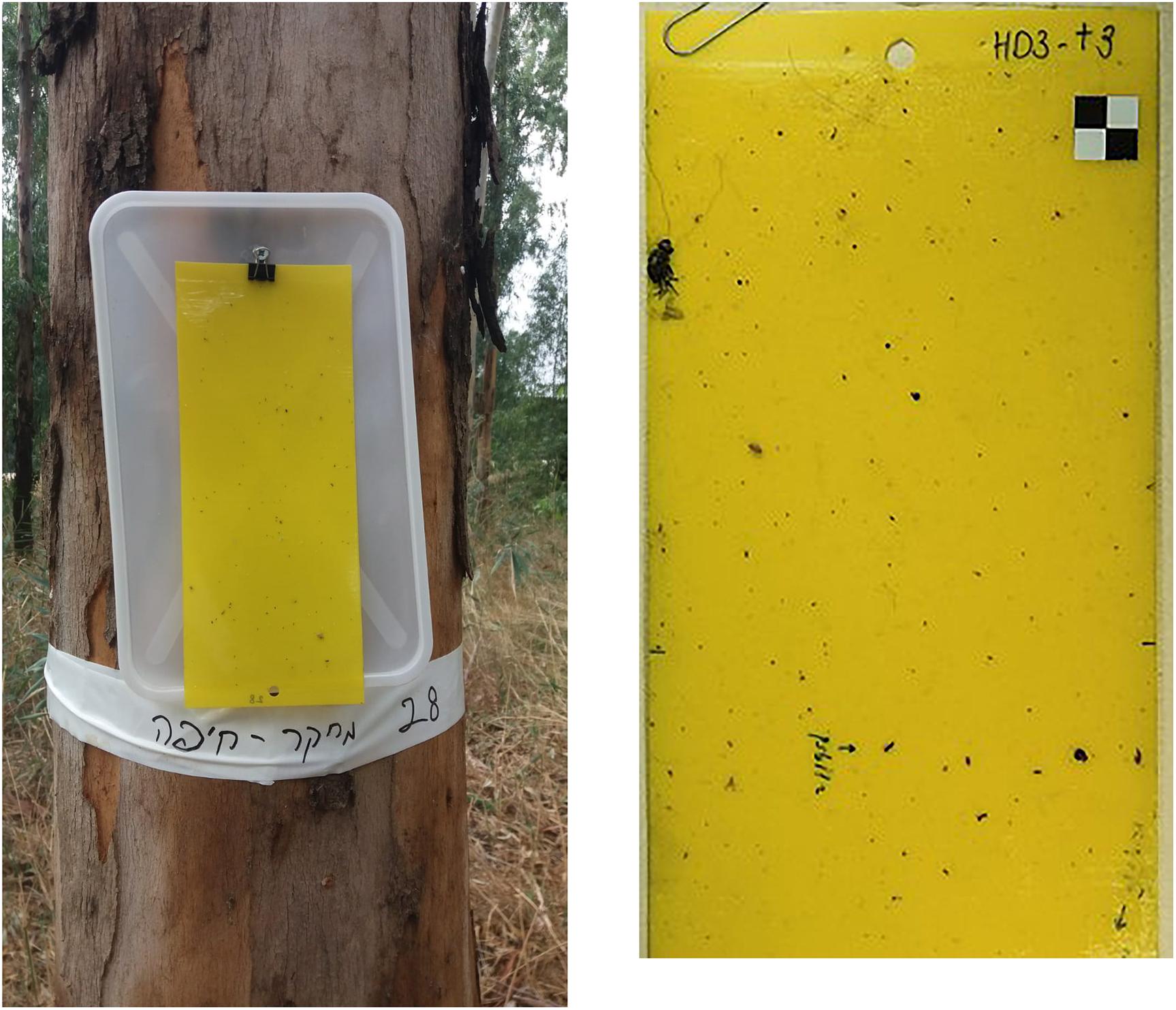
Figure 1. Left – example of a sticky trap attached to a Eucalyptus trunk. Right – image of a trap with a checkers target. A G. brimblecombei psyllid is marked with an arrow. Numerous other insects were captured, including flies, mosquitoes, and thrips.

Materials and Methods

The Model System: Invasive Insects in Israel’s Eucalyptus Forests

Background: Eucalyptus is an Australian genus that comprises more than 700 species, several of which have been introduced into afforestations around the world. The trees are valuable as sources of timber, as ornamentals and as means to reduce soil erosion. Eucalyptus plantings in Israel are dominated by Eucalyptus camaldulensis, alongside ∼180 additional species. Several herbivorous insects of Australian origin have become invasive during the last decades and are now considered widespread Eucalyptus pests. Sap-feeding hemipterans that infest leaves and young stems are part of this pest assemblage. They damage the trees directly though feeding, and indirectly through secretion of honeydew, which favors the development of sooty mold.

Our study focuses on two sap-sucking Eucalyptus pests that are globally invasive. The first, the bronze bug Thaumastocoris peregrinus, was first documented in Israel in 2014, and is mostly active in summer (Novoselsky and Freidberg, 2016). The second is the Eucalyptus redgum lerp psyllid, Glycaspis brimblecombei, recognized as a pest of economic importance in the New World and also common in several Mediterranean countries. It is active year-round, reaching high densities during May–August (Laudonia et al., 2014; Boavida et al., 2016; Mannu et al., 2019). G. brimblecombei is one of three species of Eucalyptus psyllids that have been described from Israel over the last 20 years (Spodek et al., 2015, 2017).

We also included the parasitoid wasp Psyllaephagus bliteus (Hymenoptera: Encyrtidae) in our study, as a third invasive insect of Australian origin in Eucalyptus forests. This wasp is also G. brimblecombei’s main natural enemy. P. bliteus has spontaneously established in Israel during the last decade, probably tracking the spread of its host. It oviposits on the psyllid’s nymphs, preferably in their third and fourth instars. The parasitoid’s development is delayed until the host reaches the late fourth or early fifth instar, and the parasitized psyllids die and mummify when P. bliteus begins to pupate (Daane et al., 2005).

We have recently completed a large field survey to characterize the population dynamics of these three insects under a range of climate conditions and vegetation characteristics of Eucalyptus forests (e.g., tree density and understory plant density). This still-ongoing project aims to form forestry management recommendations for reducing the pests’ infestation, and to predict the eventual distribution of these recent invasive species in Israel. Here, we describe and evaluate the monitoring protocol developed for our study. The present article thus focuses on a general methodology that can hopefully be applied to many future projects, rather than on the ecological insights arising from our specific case study. Nevertheless, we use a small subset of our field data to evaluate how well the automated image identification captures differences in insect abundances between study populations.

Insect Trapping

Insects were trapped in seven Eucalyptus forests in Israel’s coastal plain, in 2019 and 2020 (Table 1). Yellow sticky traps (25 × 10 cm) were hung on the tree trunks, at 1.5 m height, for 4–7 days.

TABLE 1

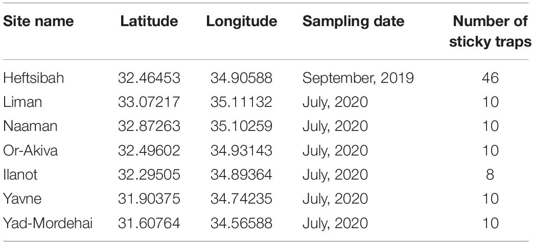
Table 1. Locations, dates, and numbers of sticky traps analyzed for this study.

Preparation of an Image Dataset

The traps were inspected by an expert entomologist under a dissecting microscope, and relevant insects (T. peregrinus bugs, G. brimblecombei psyllids, and P. bliteus parasitoids) were identified. Images of the traps were taken with a Canon 750D camera, with a kit lens of 18–55 mm. The camera was placed on a tripod, perpendicular to the traps, at 40 cm height. This height was found as ideal for capturing most of the trap in the frame (∼80%), while individual insects could still be clearly identified. Focusing was done manually using a checkers target (1.2 cm²) which was placed on the trap prior to image acquisition (Figure 1, right). Images were processed with the CoLabeler software version 2.0.4². As expected from images of field traps, they were cluttered with many irrelevant objects (i.e., leaves and other insects). We marked a rectangular polygon (bounding box, aka area of interest) around each relevant insect, from the edge of the head to the edge of the abdomen and labeled it as either “Glycaspis,” “Psyllaephagus,” or “Thaumastocoris.” These rectangles are relatively small compared with the overall size of the image. YOLOv5, the detection algorithm that we used (see below), tends to ignore such objects, thus we split the images into segments of 500 × 500 pixels. Overall, the image dataset contained 520 “Glycaspis,” 161 “Psyllaephagus,” and 67 “Thaumastocoris” manually labeled objects. These labeled boxes are considered the ground truth for the following image analysis steps.

Supervised Learning

Given an unlabeled image, the detection algorithm aims to predict the bounding boxes that an expert would have marked, and to label them correctly. For the training and testing of the method we used labeled images, which were divided to three subsets: “training,” “validation,” and “test.” In the training phase the algorithm uses the “training” and “validation” sets to create a statistical model. In the test phase we apply the model to the “test” set images, ignoring their labels. Each predicted label is associated with a confidence score that considers both the probability that the label is correct, and the expected overlap between the ground truth bounding box and the predicted one. This overlap is expressed as the Intersection over union (IoU), indicating the agreement between a predicted bounding box and a ground truth box (Eq. 1).

$$IoU=\frac{area(B_p\cap B_{gt})}{area(B_{p}U{B}_{gt})}(1)$$

where B_p and B_gt are the predicted and ground truth bounding boxes, respectively.

For example, if a box is labeled as “Glycaspis,” a high confidence score (above a predefined threshold T_cs) suggests that (a) the box indeed encloses the whole object, and that (b) the psyllid G. brimblecombei appears within, and not any other object such as a leaf or another insect. Thus, a successful prediction, true positive (TP), is a bounding box with a confidence score above T_cs and an IoU of 0.5 or higher with an expert-tagged box carrying the same class label.

The Deep Learning Network

For machine learning we used an open source implementation³ of YOLO version 5 (Ren et al., 2015; Redmon and Farhadi, 2017, Redmon and Farhadi, 2018). This algorithm simultaneously predicts bounding boxes around objects (insects, in this case) within the image, their class labels (species) and confidence scores. To this end, the algorithm generates uniformly spaced tentative bounding boxes, adjusts them (by changing their center and dimensions) to nearby objects, and assigns them a class label and confidence score. This process is governed by a loss function that penalizes high-confidence wrong predictions (wrong class or small IoU) and low-confidence correct ones. Bounding boxes of low confidence, and ones that share an object with a higher confidence box, are discarded. Typically, some classes, here “Glycaspis,” are more frequent than the others. This so-called class-imbalance may lead to overestimation of these classes. To cope with this problem, YOLOv5 automatically modifies its loss function to assign heavier weights to the less frequent classes (Lin et al., 2017). To improve performance, the YOLOv5 model is distributed after pre-training to a standard set of object images [common objects in daily contexts (COCO)⁴ ]. We subsequently trained it to the specific object identification tasks of our study.

Model Training

Deep learning models learn data iteratively: generating predictions of the training set samples, evaluating them by the loss function, and modifying their parameters according to the loss function’s gradient. Thus, the loss declines in each training round (aka epoch), and the model’s annotation accuracy increases (Figure 2 and Supplementary Figure 1). As the number of parameters of a typical deep learning model is large, overfitting is a major concern. A common (partial) remedy is the use of validation data, which are set-aside while training, yet their annotations by the models are monitored. The validation data help to limit the training duration, thereby reducing the risk of overfitting. In this study we used 30 epochs per training task, based on our validation runs (Figure 2).

FIGURE 2

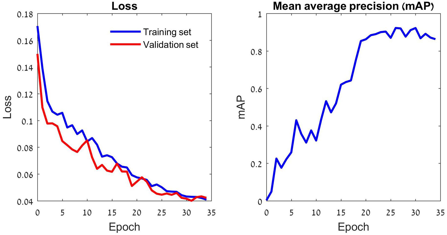
Figure 2. The training process of the YOLOv5 model. The left panel depicts the loss function that drives the learning process. This function penalizes incorrect predictions of the three focal species as well as missed ones. The learning consists of iterative reduction of this penalty for the training set images (blue) by a stochastic gradient algorithm (Ruder, 2016). The validation set images (red) do not participate in the optimization and the gradual reduction in their loss indicates that the training has not reached an overfitting point. The validation loss stabilizes after 30 epochs, suggesting that further training might lead to overfitting. Thus, the deep learning model generated by 30 training epochs was used for tests. A different perspective on the gradually improving performance of the model is provided in the right panel. The model’s average precision (AP) improves with the number of training epochs. The plot depicts the model’s mean AP (mAP) over the three insect classes.

The data of this study are images of sticky traps that we split into three sets: training, validation and test (70, 15, and 15% of the images, respectively). Table 2 reports the numbers of individual insects assigned to each of the three datasets.

TABLE 2

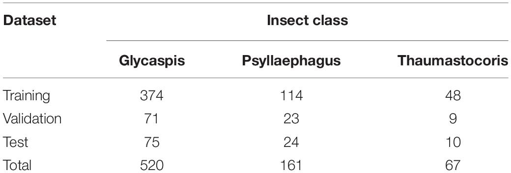
Table 2. The numbers of individuals used for training, validation, and testing of the deep learning model.

Model Evaluation

We evaluated the quality of the model by comparing the predictions with the ground truth, which is a set of boxes drawn and labeled by a human expert (magenta boxes in Figure 3). The metrics of model quality are based on the class labels and their associated confidence scores. We calculated three out of the four elements of a confusion matrix: false positives (FP), false negatives (FN) and true positives (TP). To do so, we counted boxes labeled either by the model, the expert, or both of them. We defined two thresholds: T_IoU – the lowest IoU that we consider meaningful object detection, and T_cs, the lowest confidence score that we consider reliable. Here we adopt a T_IoU of 0.5 which is commonly used in the image processing world (Everingham et al., 2010). Varying T_cs over the 0 to 1 range results in different TP, FP, and FN values, depending on how restrictive our prediction is. A prediction is considered TP if it shares a label with an observed object, their IoU is above T_IoU and the confidence score is above T_cs. A prediction with a confidence score above T_cs that misses either the identity or the location of the object is considered a false positive. Finally, a ground truth object that is not predicted (because it was incorrectly identified, or identified with below-threshold confidence) is considered a false negative. Note that the last element of the traditional confusion matrix, which is the true negatives (TN), is irrelevant here. Typically, TN represents objects that are correctly labeled as not belonging to a given class. However, in our case this corresponds to parts of the sticky trap that are not marked by any labeled rectangle, such as the yellow background and irrelevant objects. These areas are not countable.

FIGURE 3

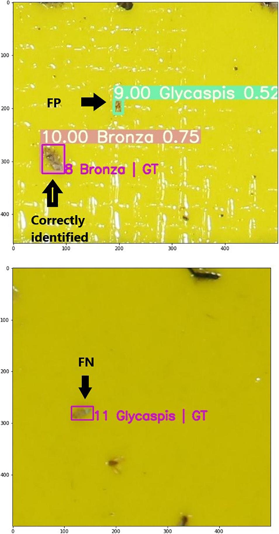
Figure 3. Two images from the test set with ground truth (GT, magenta) bounding boxes, and predicted ones (green). Each box is labeled by its class. The predicted boxes are also annotated by a confidence score. The top image demonstrates a correct identification of a bronze bug (true positive), and a false positive prediction of a Glycaspis psyllid. The bottom image demonstrates a false negative result, namely a Glycaspis individual annotated by the human expert but not detected with the machine-learning model.

We evaluated the performance of the model separately for each class, using precision and recall (PR) curves. Recall (Eq. 2) is the fraction of relevant objects that were correctly classified. In our case, it is the proportion of expert-labeled “Glycaspis” (respectively “Psyllaephagus” or “Thaumastocoris”) objects that were also labeled “Glycaspis” (respectively “Psyllaephagus” or “Thaumastocoris”) by the deep learning model. Recall is defined as the number of true positives divided by the sum of true positives and false negatives. Precision (Eq. 3) is the fraction of correctly classified objects among all classified objects. It is defined as the number of true positives divided by the sum of true positives and false positives:

$$\text{Recall}=\frac{TP}{TP+FN}(2)$$

$$\text{Precision}=\frac{TP}{TP+FP}(3)$$

By setting the threshold for confidence score at different levels, we get different pairs of PR values, which form the PR curve (Figure 4).

FIGURE 4

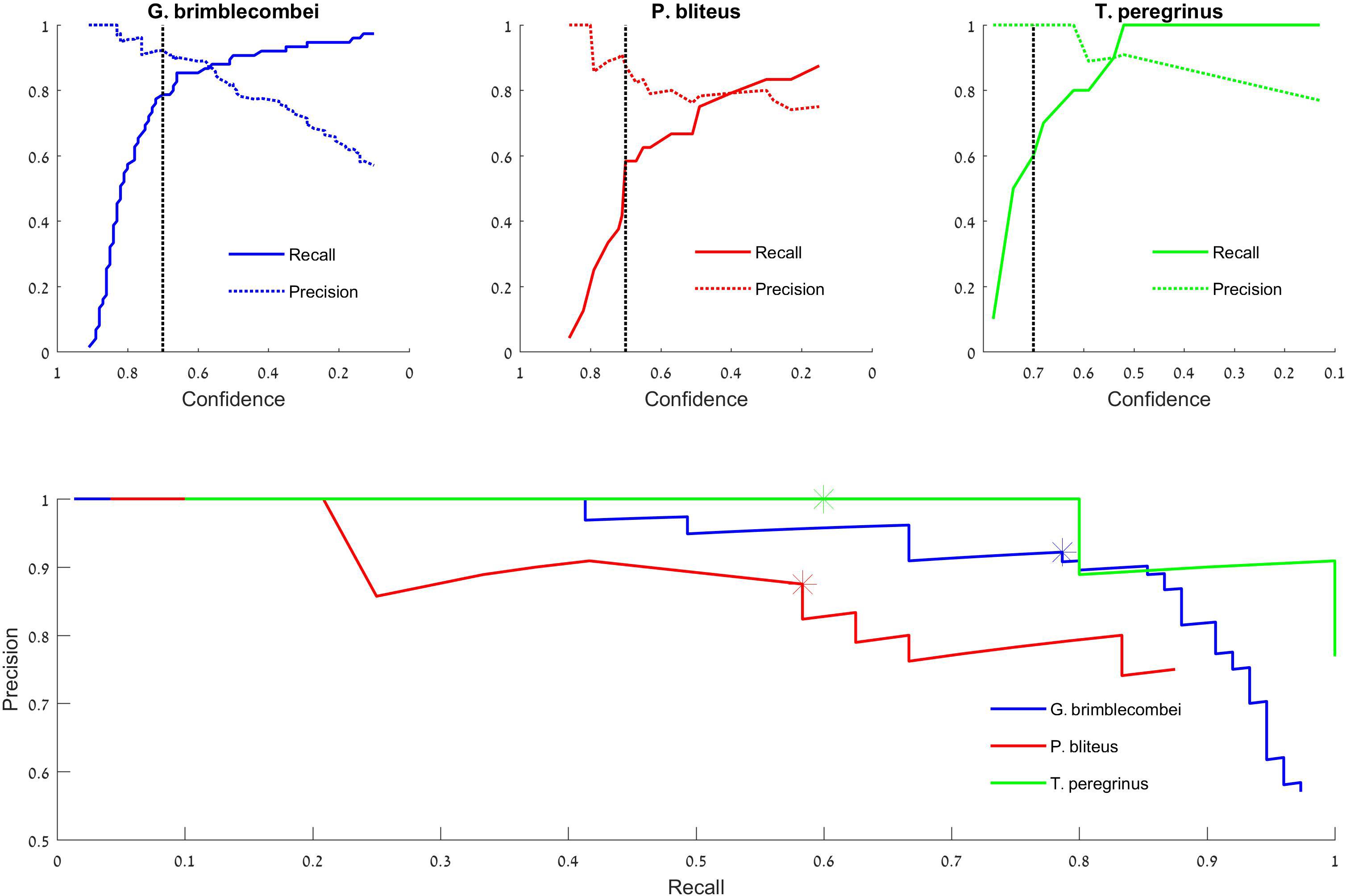
Figure 4. Test set precision-recall curves. Top: the model’s success in identifying “Glycaspis” vs. “non-Glycaspis” (left), “Psyllaephagus” vs. “non-Psyllaephagus” (middle), and “Thaumastocoris” vs. “non-Thaumastocoris” (right). The plots indicate the recall and precision of the model’s predictions as a function of its confidence threshold (T_cs). The black dotted line depicts 0.7 confidence. Bottom: Recall vs. Precision curves of the three focal species. Asterisks depict a confidence threshold of 0.7. Note that the recall plots of “Glycaspis” and “Psyllaephagus” do not reach 1, as a few insects were not identified even with T_cs = 0.1.

We used the average precision, over all observed recall values, as a single model-performance metric, which takes into account the trade-off between precision and recall. Precision values, and hence also their average, range between 0 and 1. The average precision of an ideal predictive model equals 1, meaning it always detects every class correctly. As this value decreases, so does the performance of the model.

Preliminary Application to Forest Ecology Research

We used the samples of 2020 to test how well the machine-learning model captures insect abundance variability in “real-life” data. A total of 58 traps, set up in July 2020 in six research sites, served as the dataset (Table 1). The three focal insects were tagged on all images by an expert. Nineteen traps that did not contain any of these species of interest were excluded from further analysis. The remaining 39 traps were subjected to the machine-learning model in 39 rounds. In each round, we assigned one trap image to the test set and trained the model on the remaining 38 trap images as well as on the images from the 2019 samples. This procedure allowed us to compare the insects’ per-site abundance based on expert identification vs. model prediction.

Results

Trapping of Forest Insects

Both the psyllid (class “Glycaspis”) and its parasitoid (class “Psyllaephagus”) were trapped in all seven sampling sites, both in 2019 and in 2020. The psyllid, however, was much more common on the traps. Bronze bugs (class “Thaumastocoris”) were captured in a single site in 2020 only. Numerous other insects were trapped as well, mostly flies, mosquitoes, and thrips, but also other psyllids, parasitoids, and true bugs. These insects were not identified or counted. The optimal trapping duration (resulting in ∼50% of the trap surface covered with insects) was 1 week.

Automatic Insect Detection

Model Evaluation

We report our results on the test set. The detection of “Glycaspis,” “Psyllaephagus,” and “Thaumastocoris” resulted in average precision values of 0.92, 0.77, and 0.97, respectively. Thus, the model performed well on both pests, and was less successful in identifying the parasitoid. A detailed evaluation of the model’s performance is provided in Figure 4. The top panels depict the performance of the model as a function of its stringency (the confidence score threshold). The difference performance measures are plotted separately for the three identification tasks. For all tasks, as the model becomes more permissive (i.e., requires a lower confidence score to make a decision), it makes more true positive and fewer false negative identifications. On the other hand, the number of false positive identifications increases as well. The optimal confidence threshold needs to be selected by the model’s users according to the ecological task at hand. For example, a low threshold can be desirable for monitoring of disease-vectoring insects. This would enable early detection and control of the pests, at the cost of some false alarms (false positive identifications). A higher threshold may be suitable for other aims, such as describing the seasonal dynamics of our forest insects. In this case, one might favor high accuracy (few FPs) over completeness of identification (few FNs).

The tradeoff between FP and FN errors is formulated in the concepts of recall and precision (Eqs 2 and 3, respectively), and is visualized by a Precision-Recall plot (Figure 4 bottom). Each data point on this plot depicts the recall (x-coordinate) and precision (y-coordinate) associated with a particular confidence score (T_cs). Confidence scores decrease along the X-axis. Thus, the leftmost data points denote the proportion of insects detected (recall), and the fraction of predictions that are correct (precision), when the highest confidence level (1) is used by the model. The rightmost data points describe the performance attained by a model that accepts all identifications, as its T_cs is minimal (0). Such a plot can guide users in adjusting model parameters to their needs. If fewer detections are accepted (low recall), precision increases.

Tables 3, 4 illustrate the types of recall (Table 3) and precision (Table 4) errors made by the model when the confidence threshold was set to 0.7. The model rarely confused between our three focal species (gray areas in Tables 3, 4). It made some false positive predictions, particularly for the class “Psyllaephagus” (bold text in Table 4, not tagged by the expert but predicted by the model). Most of the missed predictions, however, were false negatives (bold text in Table 3, tagged by the expert but not identified by the model).

TABLE 3

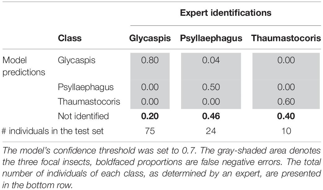
Table 3. Proportions of correct (recall) and erroneous predictions of each insect class, out of their total numbers in the test set.

TABLE 4

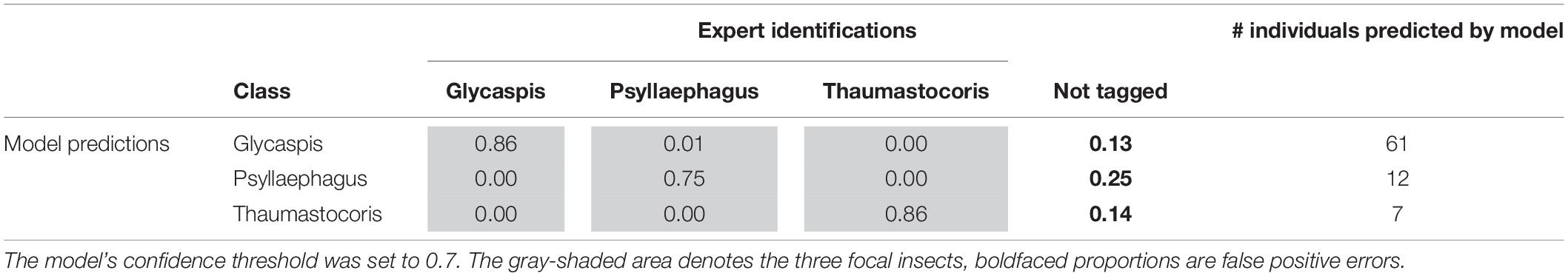
Table 4. Proportions of correct (precision) and erroneous predictions in the test set, out of the total number of individuals from each insect class that were predicted by the machine learning model.

Preliminary Application to Forest Ecology Research

To test the utility of our approach in a real-world scenario we compared the ability of insect identifications, by either an expert or the deep learning algorithm, to address two simple yet biologically relevant questions. First, do the per-site abundances of our study species show any latitudinal pattern, say due to a climate gradient; and second, are the populations of the three species correlated in abundance, i.e., are any sites particularly attractive for all the species in our study. Figure 5 summarizes the per-site abundances of the three focal species. Sites are ordered from north to south. Expert counts of individual trapped insects (filled bars) are shown next to the deep-learning based predictions (striped bares), using a confidence threshold of 0.7. Evidently, by both counting techniques none of the populations followed a clear north-south pattern. Further, both methods show that “Glycaspis” and “Psyllaephagus” were relatively common in two non-adjacent sites (Yad-Mordehai and Or-Akiva), while a single “Thaumastocoris” population occurred in a third site (Naaman). Both counting methods also suggest comparable correlation coefficients between the per-site abundances of “Glycaspis” and “Psyllaephagus,” 0.72 vs. 0.65 for expert-based counts and software-based counts, respectively.

FIGURE 5

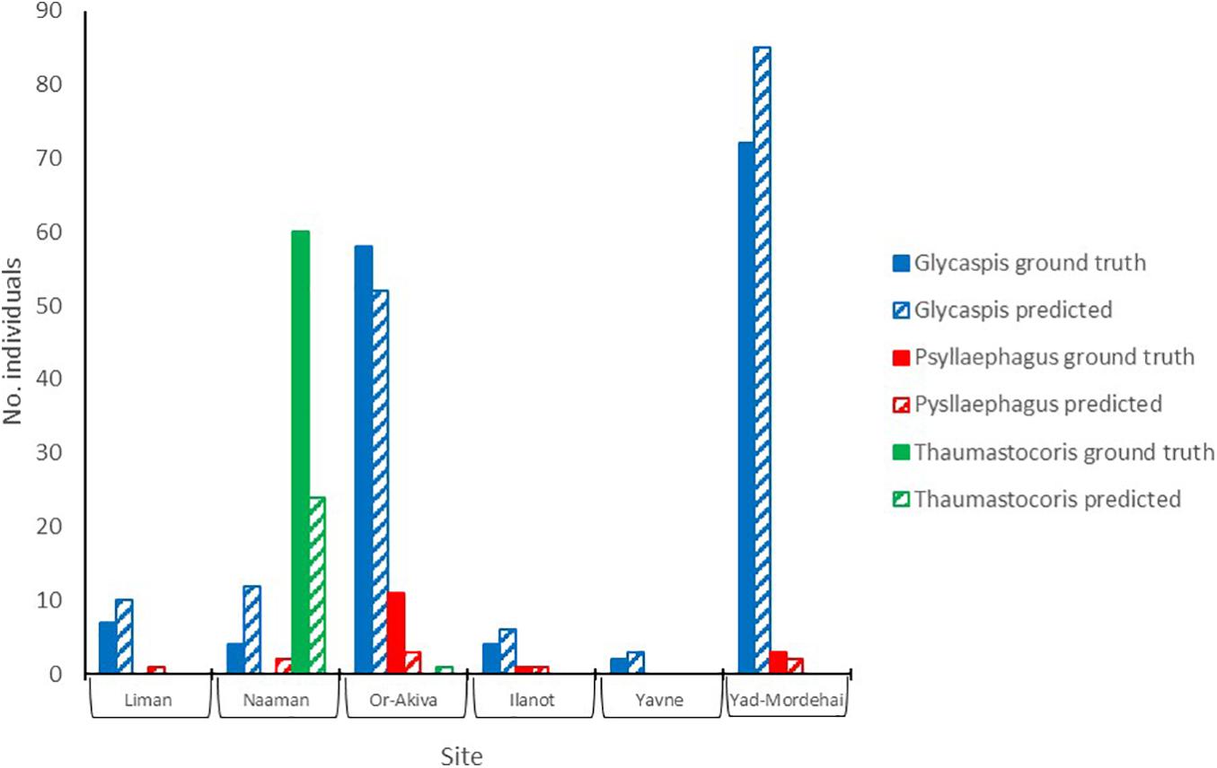
Figure 5. Counts of “Glycaspis” (blue) “Psyllaephagus” (red), and “Thaumastocoris” (green) from sticky traps, as evaluated by a human expert (filled bars) and predicted by the deep-learning model (hatched bars). The traps were placed in six Eucalyptus forests along Israel’s coastal plain in July 2020. Trapping sites are ordered from north to south. See Table 1 for location details and sample sizes.

Discussion

The current study tested the feasibility of training a deep learning model to identify three insect classes of interest on images of sticky traps. As the insects are rather small, require discrimination from many non-focal objects caught on the same traps, and stick to the traps in random poses, the prospects of success were not obvious. Given these challenges, the positive results of our test are non-trivial and encouraging. Moreover, the model achieved high detection and classification performance even with a very small training dataset. These model evaluation results, as summarized in Figures 2, 4 and Tables 3, 4, are independent of the ecological questions that we are addressing.

The model’s performance varied between the different identification tasks. The object class “Glycaspis” was predicted with high recall and precision, while class “Thaumastocoris” scored high on precision but lower on recall. Class “Psyllaephagus” had the lowest prediction success in both recall and precision (Tables 3, 4). In all three classes, false negative prediction errors were more common than false positive errors. That is, the model was more prone to miss relevant images than to include irrelevant ones. Training the model on larger repositories of tagged images, and using higher-quality photos, will likely reduce both types of errors in future work.

“Glycaspis” images were much more common in our dataset than the other two insect classes. Such class imbalance is a potential concern because it might cause the machine-learning model to over-learn and over-predict the most common class. Yet, in our test set, “Psyllaephagus” was mis-predicted as “Glycaspis” in only 4% of cases, and none of the “Thaumastocoris” images were falsely predicted as “Glycaspis.” More generally, the model rarely confused between the three insect classes to which it had been trained. We conclude that class imbalance was not a major constraint on model quality in our case, possibly because the YOLOv5 algorithm efficiently corrected for it (Lin et al., 2017).

After evaluating our method’s general performance, we also tested it in the context of our case study, which deals with insect population dynamics in Eucalyptus forests. Over the spring and summer of 2020, we conducted six insect sampling sessions in each of 15 Eucalyptus forests, located along a climatic gradient in coastal Israel. We placed 30 sticky traps in different parts of each forest in each sampling session and recovered them a week later. In the present work, we analyzed a small subset of these traps (58 traps from six sites and a single sampling month) to test how well the deep learning model detects between-site differences in insect abundances. We found that the per-site abundances, estimated by both an expert and our deep learning algorithm, show no clear pattern with respect to the north-south axis. Both counting methods indicated considerable correlation between the abundances of “Psyllaephagus” and “Glycaspis,” while class “Thaumastocoris” had a very aggregated distribution. Having established the utility of our computational approach, we are now aiming to use the model to extract the abundances of G. brimblecombei, P. bliteus, and T. peregrinus from the complete dataset of trap images, to describe their population trends in time and space. We will also analyze the effects of tree density, forest understory composition, and climatic variables on the abundance of these invasive insects. This information will help to predict their eventual establishment in Israel and to form recommendations for their management.

Being a proof-of-concept project, with rather limited resources, our present work comprises a small-scale case study, namely monitoring two forest pests and one natural enemy. Its success, as well as the results of a few other recent studies (reviewed by Høye et al., 2021), suggest that computer vision-based analysis of sticky trap images may have additional major contributions to insect ecoinformatics, and entomology in general. An obvious future direction is to extend the current studies to multiple additional insect species of interest, over larger spatial and temporal ranges. A parallel computational effort is needed to adjust the machine-learning algorithms to the peculiarities of sticky-trap images. For example, the current studies use off-the-shelf object detection algorithms. These, however, were developed to detect common objects in daily contexts (COCO). Sticky trap images are very different, and their study may benefit from the development of more tailored algorithms.

Most insect capture methods, sticky traps included, are non-selective, and therefore inevitably capture many non-target arthropods (pheromone traps are notable exception). Thus, the design of every such study should include conservation considerations such as avoiding trapping in breeding habitats or along migration routes of endangered insects. Unlike other methods, sticky trap images allow insects, which are considered bycatch for a particular research or monitoring project, to become focal species for other ventures, reducing the overall environmental load of such studies. This requires a centralized free repository that will house image datasets. Such a repository will trigger further studies, including retrospective ones that will exploit the available rich image data.

Looking forward, we believe that the utility of sticky trap images may well be extended beyond estimation of species abundances. Demographic and life history traits, for example, sex ratios and age group distributions, may be inferred from morphological attributes such as body sizes and allometric relationships between body parts. These attributes may be extracted from trap images, and allow the study of habitat effect on these traits. Thus, computational analysis of sticky trap images will soon allow many ecological applications that are now practically impossible. These include early detection of the arrival of invasive species, disease vectors or crop pests into new areas; identification of insect migration pathways to allow effective design of ecological corridors; and predicting climate-change effects by insect densities, activity seasons, body sizes, age distributions, and sex ratios along climatic gradients.

Data Availability Statement

The trap images and the associated programming code are available online at http://meshi1.cs.bgu.ac.il/FIE2020_data.

Author Contributions

CK, AB-M, AS, and TK conceptualized the project. CK, AG, and VW developed the deep learning model. AS sampled the insects and prepared annotated images. CK and TK wrote the manuscript. All authors reviewed the manuscript, added their inputs, approved the final version of the manuscript, and agreed to be held accountable for its content.

Funding

This work was supported by the Data Science Research Center, University of Haifa, and by the Zoological Society of Israel. It was also partially supported by the Israeli Council for Higher Education (CHE) via Data Science Research Center and Ben-Gurion University of the Negev, Israel.

Conflict of Interest

The authors declare that the research was conducted in the absence of any commercial or financial relationships that could be construed as a potential conflict of interest.

Supplementary Material

The Supplementary Material for this article can be found online at: https://www.frontiersin.org/articles/10.3389/fevo.2021.600931/full#supplementary-material

Supplementary Figure 1 | The model’s loss function (Figure 2 left panel) is a sum of three components, each of which penalizes a different type of prediction error: incorrectly placed bounding boxes (left panel), failures in detecting an object (center panel), and failures in correctly identifying it (right panel). All three components decrease during training and validation.

Footnotes

1. ^ https://www.gbif.org
2. ^ http://www.colabeler.com
3. ^ https://github.com/ultralytics/yolov5/tree/v4.0
4. ^ https://cocodataset.org/#home

References

Bjorkman, C., and Niemela, P. (2015). Climate Change and Insect Pests, Vol. 8. Wallingford: CABI.

Google Scholar

Boavida, C., Garcia, A., and Branco, M. (2016). How effective is Psyllaephagus bliteus (Hymenoptera: Encyrtidae) in controlling Glycaspis brimblecombei (Hemiptera: Psylloidea)? Biol. Cont. 99, 1–7. doi: 10.1016/j.biocontrol.2016.04.003

CrossRef Full Text | Google Scholar

Buschbacher, K., Ahrens, D., Espeland, M., and Steinhage, V. (2020). Image-based species identification of wild bees using convolutional neural networks. Ecol. Inform. 55:101017. doi: 10.1016/j.ecoinf.2019.101017

CrossRef Full Text | Google Scholar

Cheng, X., Zhang, Y., Chen, Y., Wu, Y., and Yue, Y. (2017). Pest identification via deep residual learning in complex background. Comput. Electron. Agric. 141, 351–356. doi: 10.1016/j.compag.2017.08.005

CrossRef Full Text | Google Scholar

Chudzik, P., Mitchell, A., Alkaseem, M., Wu, Y., Fang, S., Hudaib, T., et al. (2020). Mobile real-time grasshopper detection and data aggregation framework. Sci. Rep. 10:1150.

Google Scholar

Cuthill, J. F. H., Guttenberg, N., Ledger, S., Crowther, R., and Huertas, B. (2019). Deep learning on butterfly phenotypes tests evolution’s oldest mathematical model. Sci. Adv. 5:eaaw4967. doi: 10.1126/sciadv.aaw4967

PubMed Abstract | CrossRef Full Text | Google Scholar

Daane, K. M., Sime, K. R., Dahlsten, D. L., Andrews, J. W. Jr., and Zuparko, R. L. (2005). The biology of Psyllaephagus bliteus Riek (Hymenoptera: Encyrtidae), a parasitoid of the red gum lerp psyllid (Hemiptera: Psylloidea). Biol. Cont. 32, 228–235. doi: 10.1016/j.biocontrol.2004.09.015

CrossRef Full Text | Google Scholar

Dainese, M., Martin, E. A., Aizen, M. A., Albrecht, M., Bartomeus, I., Bommarco, R., et al. (2019). A global synthesis reveals biodiversity-mediated benefits for crop production. Sci. Adv. 5:eaax0121.

Google Scholar

Everingham, M., Van Gool, L., Williams, C. K., Winn, J., and Zisserman, A. (2010). The pascal visual object classes (voc) challenge. Int. J. Comput. Vis. 88, 303–338. doi: 10.1007/s11263-009-0275-4

CrossRef Full Text | Google Scholar

Ezray, B. D., Wham, D. C., Hill, C. E., and Hines, H. M. (2019). Unsupervised machine learning reveals mimicry complexes in bumblebees occur along a perceptual continuum. Proc. R. Soc. Lond. B 286:20191501. doi: 10.1098/rspb.2019.1501

PubMed Abstract | CrossRef Full Text | Google Scholar

Gueta, T., and Carmel, Y. (2016). Quantifying the value of user-level data cleaning for big data: a case study using mammal distribution models. Ecol. Inform. 34, 139–145. doi: 10.1016/j.ecoinf.2016.06.001

CrossRef Full Text | Google Scholar

Hallmann, C. A., Sorg, M., Jongejans, E., Siepel, H., Hofland, N., Schwan, H., et al. (2017). More than 75 percent Haline over 27 years in total flying insect biomass in protected areas. PLoS One 12:e0185809. doi: 10.1371/journal.pone.0185809

PubMed Abstract | CrossRef Full Text | Google Scholar

Hansen, O. L., Svenning, J. C., Olsen, K., Dupont, S., Garner, B. H., Iosifidis, A., et al. (2020). Species−level image classification with convolutional neural network enables insect identification from habitus images. Ecol. Evol. 10, 737–747. doi: 10.1002/ece3.5921

PubMed Abstract | CrossRef Full Text | Google Scholar

Hickling, R., Roy, D. B., Hill, J. K., Fox, R., and Thomas, C. D. (2006). The distributions of a wide range of taxonomic groups are expanding polewards. Glob. Change Biol. 12, 450–455. doi: 10.1111/j.1365-2486.2006.01116.x

CrossRef Full Text | Google Scholar

Høye, T. T., Ärje, J., Bjerge, K., Hansen, O. L., Iosifidis, A., Leese, F., et al. (2021). Deep learning and computer vision will transform entomology. Proc. Natl. Acad. Sci. U.S.A. 118:e2002545117.

Google Scholar

Laudonia, S., Margiotta, M., and Sasso, R. (2014). Seasonal occurrence and adaptation of the exotic Glycaspis brimblecombei Moore (Hemiptera: Aphalaridae) in Italy. J. Nat. Hist. 48, 675–689. doi: 10.1080/00222933.2013.825021

CrossRef Full Text | Google Scholar

Lin, T. Y., Goyal, P., Girshick, R., He, K., and Dollár, P. (2017). “Focal loss for dense object detection,” in Proceedings of the IEEE International Conference on Computer Vision, (Cambridge, MA: IEEE), 2980–2988.

Google Scholar

Lister, B. C., and Garcia, A. (2018). Climate-driven declines in arthropod abundance restructure a rainforest food web. Proc. Natl. Acad. Sci. U.S.A. 115, E10397–E10406.

Google Scholar

Liu, L., Wang, R., Xie, C., Yang, P., Wang, F., Sudirman, S., et al. (2019). PestNet: an end-to-end deep learning approach for large-scale multi-class pest detection and classification. IEEE Access 7, 45301–45312. doi: 10.1109/access.2019.2909522

CrossRef Full Text | Google Scholar

Mannu, R., Buffa, F., Pinna, C., Deiana, V., Satta, A., and Floris, I. (2019). Preliminary results on the spatio-temporal variability of Glycaspis brimblecombei (Hemiptera Psyllidae) populations from a three-year monitoring program in Sardinia (Italy). Redia 101:7.

Google Scholar

McKinney, M. L. (2002). Urbanization, biodiversity, and conservation. Bioscience 52, 883–890. doi: 10.1641/0006-3568(2002)052[0883:ubac]2.0.co;2

CrossRef Full Text | Google Scholar

Miao, Z., Gaynor, K. M., Wang, J., Liu, Z., Muellerklein, O., Norouzzadeh, M. S., et al. (2019). Insights and approaches using deep learning to classify wildlife. Sci. Rep. 9:8137.

Google Scholar

Nieuwenhuizen, A. T., Hemming, J., and Suh, H. K. (2018). Detection and Classification of Insects on Stick-Traps in a Tomato Crop Using Faster R-CNN. Berlin: Researchgate.

Google Scholar

Novoselsky, T., and Freidberg, A. (2016). First record of Thaumastocoris peregrinus (Hemiptera: Thaumastocoridae) in the Middle East, with biological notes on its relations with eucalyptus trees. Isr. J. Entomol. 46, 43–55.

Google Scholar

Redmon, J., Divvala, S., Girshick, R., and Farhadi, A. (2016). “You only look once: unified, real-time object detection,” in Proceedings of the IEEE Conference on Computer Vision and Pattern Recognition, (San Juan, PR: IEEE), 779–788.

Google Scholar

Redmon, J., and Farhadi, A. (2017). “YOLO9000: better, faster, stronger,” in Proceedings of the IEEE Conference on Computer Vision and Pattern Recognition, (San Juan, PR: IEEE), 7263–7271.

Google Scholar

Redmon, J., and Farhadi, A. (2018). Yolov3: an incremental improvement. arXiv [Preprint] arXiv:1804.02767

Google Scholar

Ren, S., He, K., Girshick, R., and Sun, J. (2015). “Faster r-cnn: towards real-time object detection with region proposal networks,” in Advances in Neural Information Processing Systems, eds M. I. Jordan, Y. LeCun, and S. A. Solla (Cambridge, MA: MIT Press), 91–99.

Google Scholar

Roosjen, P. P., Kellenberger, B., Kooistra, L., Green, D. R., and Fahrentrapp, J. (2020). Deep learning for automated detection of Drosophila suzukii: potential for UAV−based monitoring. Pest Manag. Sci. 76, 2994–3002. doi: 10.1002/ps.5845

PubMed Abstract | CrossRef Full Text | Google Scholar

Rosenheim, J. A., and Gratton, C. (2017). Ecoinformatics (big data) for agricultural entomology: pitfalls, progress, and promise. Ann. Rev. Entomol. 62, 399–417. doi: 10.1146/annurev-ento-031616-035444

PubMed Abstract | CrossRef Full Text | Google Scholar

Rosenheim, J. A., Parsa, S., Forbes, A. A., Krimmel, W. A., Hua Law, Y., Segoli, M., et al. (2011). Ecoinformatics for integrated pest management: expanding the applied insect ecologist’s tool-kit. J. Econ. Entomol. 104, 331–342. doi: 10.1603/ec10380

PubMed Abstract | CrossRef Full Text | Google Scholar

Ruder, S. (2016). An overview of gradient descent optimization algorithms. arXiv [Preprint] arXiv:1609.04747

Google Scholar

Sánchez-Bayo, F., and Wyckhuys, K. A. (2019). Worldwide decline of the entomofauna: a review of its drivers. Biol. Cons. 232, 8–27. doi: 10.1016/j.biocon.2019.01.020

CrossRef Full Text | Google Scholar

Short, A. E. Z., Dikow, T., and Moreau, C. S. (2018). Entomological collections in the age of big data. Ann. Rev. Entomol. 63, 513–530. doi: 10.1146/annurev-ento-031616-035536

PubMed Abstract | CrossRef Full Text | Google Scholar

Spodek, M., Burckhardt, D., and Freidberg, A. (2017). The Psylloidea (Hemiptera) of Israel. Zootaxa 4276, 301–345. doi: 10.11646/zootaxa.4276.3.1

CrossRef Full Text | Google Scholar

Spodek, M., Burckhardt, D., Protasov, A., and Mendel, Z. (2015). First record of two invasive eucalypt psyllids (Hemiptera: Psylloidea) in Israel. Phytoparasitica 43, 401–406. doi: 10.1007/s12600-015-0465-2

CrossRef Full Text | Google Scholar

Thomas, J. A., Telfer, M. G., Roy, D. B., Preston, C. D., Greenwood, J. J. D., Asher, J., et al. (2004). Comparative losses of British butterflies, birds, and plants and the global extinction crisis. Science 303, 1879–1881. doi: 10.1126/science.1095046

PubMed Abstract | CrossRef Full Text | Google Scholar

van Klink, R., Bowler, D. E., Gongalsky, K. B., Swengel, A. B., Gentile, A., and Chase, J. M. (2020). Meta-analysis reveals declines in terrestrial but increases in freshwater insect abundances. Science 368, 417–420. doi: 10.1126/science.aax9931

PubMed Abstract | CrossRef Full Text | Google Scholar

Wäldchen, J., and Mäder, P. (2018). Plant species identification using computer vision techniques: a systematic literature review. Arch. Comput. Methods Eng. 25, 507–543. doi: 10.1007/s11831-016-9206-z

PubMed Abstract | CrossRef Full Text | Google Scholar

Wu, S., Chang, C. M., Mai, G. S., Rubenstein, D. R., Yang, C. M., Huang, Y. T., et al. (2019). Artificial intelligence reveals environmental constraints on colour diversity in insects. Nature Commun. 10:4554.

Google Scholar

Zhong, Y., Gao, J., Lei, Q., and Zhou, Y. (2018). A vision-based counting and recognition System for flying insects in intelligent agriculture. Sensors. 18:1489. doi: 10.3390/s18051489

PubMed Abstract | CrossRef Full Text | Google Scholar