A Step-by-Step Guide to Initialize and Calibrate Landscape Models: A Case Study in the Mediterranean Mountains

Introduction

Forests are indispensable ecosystems for human societies. Due to their role as climate regulators, soil protectors and biodiversity hotspots, forests provide a multitude of ecosystem services and are fundamental elements in the world’s economy (Krieger, 2001; Martínez Pastur et al., 2018). The potential adverse impacts of global change on forest ecosystems emphasizes the need to understand how to manage them in the future (Lindner et al., 2014; Hof et al., 2017; Mina et al., 2017).

In recent years, the use of computational models has been increasing in forest ecosystem research (Gustafson et al., 2017; Shifley et al., 2017). Although empirical studies are of fundamental importance for process understanding, simulation models are nowadays recognized as useful tools to assess our knowledge about the functioning of ecosystems as well as essential allies when predicting future changes (Seidl, 2017). Over the past decades, a large range of models were developed to describe future dynamics in forest ecosystems (Keane et al., 2015), from stand-scale empirical simulators to more complex process-based models operating at landscape scale (Fontes et al., 2010). Because of computational constraints, models integrating fine-resolution processes (e.g., photosynthesis, specific growth functions) at large scales in a spatially explicit framework were rare, and smaller grain processes were often strongly simplified (Elkin et al., 2012). However, these constraints are constantly being reduced by the increase in computational power, allowing for the flourishing of Forest Landscape Models (FLMs) which integrate physiologically based processes from stand to landscape level (Seidl et al., 2012; De Bruijn et al., 2014; Shifley et al., 2017; Petter et al., 2020).

According to Jorgensen and Fath (2011), ecological models comprise five elements: state variables, external variables, parameters, mathematical equations, and universal constants. The mathematical equations and universal constants are implicit within the model structure, while the initial conditions of the state variables (e.g., species biomass, species age), external variables and parameter values are usually provided as inputs by the user for each simulation study. In the case of FLMs, they represent forests across the landscape in a spatially explicit way. The landscape is depicted as a set of cells for which a series of state and external variables are defined. These variables are used to define the ecological processes taking place at cell level (e.g., growth, mortality among others) and at landscape level (e.g., seed dispersal, fire spread). For comprehensive reviews on the development, structure and recent applications of FLMs see Shifley et al. (2017); Keane et al. (2015), and He et al. (2017).

The above-mentioned structural elements are essential to set up a simulation in a specific landscape. This requires the user to obtain, prepare and organise comprehensive datasets to address the two first key steps in applying FLMs: model initialization (initial conditions of state and external variables) and calibration of model parameters. The initial conditions of the state variables describe the ecosystem at the beginning of the simulation. In turn, external variables are those forces affecting the ecosystem without being internal parts of it (Jorgensen and Fath, 2011). Most FLMs require initial values of at least certain state and external variables to start a simulation. As an example, the FLM LandClim requires elevation or browsing intensity for initialization (Petter et al., 2020). In addition to biophysical conditions (e.g., soil types, climate maps or regions), essential initial conditions for FLMs are vegetation maps describing which species are present in the landscape at the beginning of the simulation time. Decisions regarding the inclusion or exclusion of certain species can be highly relevant in certain ecosystems (e.g., shrubs in the Mediterranean area). Thus, these vegetation maps are a keystone within these experiments since forest dynamics and properties (biomass, available light, regeneration, etc.) are highly driven by initial conditions and structure (Duveneck et al., 2015; Scheller and Swanson, 2015). For example, most FLMs require information of tree species and their age classes across the landscape. This information can be very challenging to obtain and estimate for large spatial scales without necessarily combining multiple and complex datasets (Zald et al., 2014). The generation of input data for FLMs can therefore require significant time and skills, and often demands complementarity with experimental research from long-term field studies (Shifley et al., 2017; Scheller, 2018).

The calibration of model parameters has been defined as one of the greatest challenges in modelling under environmental changes (Keane et al., 2015; Scheller, 2018). Model parameters are values used in model equations which represent processes (Jorgensen and Fath, 2011). Most models simulating the succession dynamics of vegetation require parameters describing the behaviour of the species present in the landscape. These parameters may differ for each model, but commonly refer to species growth characteristics, fruit and seed dispersal, reproduction strategies and absolute or relative measures of tolerance to stress factors (Huber et al., 2018). A broad range of sources can be used to fulfil these parameters, ranging from empirical case-specific data collected by the modeller to values of standard variables stored in global databases. In either case, an evaluation of model outputs to identify appropriate parameter values is usually required to ensure that the model produces plausible outcomes at the local scale (Gutiérrez et al., 2016; Duveneck et al., 2017). This evaluation of parameter values is known as calibration (Mulligan and Wainwright, 2013). During this phase, the different model sensitivity to some parameters over others should be considered (McKenzie et al., 2019).

Successional processes and long-term projections in FLM are highly sensitive to initial conditions and model parameters (Scheller, 2018). Estimation of initial condition and calibration procedures are typically described in the method section in literature studies (e.g., Scheller et al., 2005; Boulanger et al., 2017), but often not on a level of detail to allow full reproducibility or with enough information to help non-modellers to setup a new landscape from scratch. Even fewer provide access to inputs, outputs and scripts in public repositories. The aims of this study are twofold. First, documenting the process needed to initialize and calibrate a FLM step-by-step, as an example for analogous uses. Fulfilling this goal would encourage the application of FLMs as scientific tools to assess future forest dynamics and management adaptation under global change. Second, we aim at testing different initialization data – with and without shrub communities – by assessing the model ability to project forest landscape dynamics in a biome where the model has not been applied so far (Euro-Mediterranean region).

Materials and Methods

Model Description

In this manuscript, we chose LANDIS-II as our reference FLM. LANDIS-II¹ (Scheller et al., 2007) is a FLM designed to simulate forest dynamics at multiple spatial and temporal scales. It allows a wide degree of complexity depending on a set of extensions which can optionally be activated to simulate different processes such as succession, disturbances (fire, wind, herbivory, and pests) and management at different degrees of complexity (e.g., areas- and species-specific harvesting regimes, post-harvesting planting). The spatial scale (i.e., cell resolution) is defined by the user, which makes it very flexible and adaptable to a wide variety of simulation experiments. In LANDIS-II, the landscape is divided into ecoregions, which are subregions sharing similar climatic conditions and soil characteristics. Trees in each cell are represented as species-age cohorts, increasing the computational efficiency of the model (De Bruijn et al., 2014).

Particularly, we used the PnET-Succession extension v.3.4 (De Bruijn et al., 2014; Gustafson et al., 2015). This extension embeds the PnET-II ecophysiological model equations (Aber and Federer, 1992). PnET-Succession simulates forest succession in a more mechanistic way than previous approaches, representing an advantage for experiments where novel conditions such as climate change are being explored (Gustafson, 2013). In PnET-Succession, age is used to calculate cohort’s biomass at the onset of the simulation (i.e., model spin-up) and cohorts with higher biomass are given priority access to light and water (Gustafson and Miranda, 2019). Cohort biomass is assumed to be homogeneously distributed in the cell and therefore shade conditions are also homogeneous within a cell (Scheller et al., 2007). Potential net photosynthesis rate is calculated as a linear function of foliar nitrogen (FolN) and biomass growth is a result of environmental conditions such as temperature, precipitation, photosynthetically active radiation (PAR), CO₂ concentrations and—optionally—ozone concentrations (De Bruijn et al., 2014). Biomass allocation depends on compartments turnover and fraction parameters. Mortality can occur at any time if carbon reserves become limiting (non-structural carbon <1%) or when age approaches species longevity (De Bruijn et al., 2014).

PnET-Succession requires a series of generic, ecoregion- and species-specific parameters. Although many default values have been made available by the model developers and in past application studies, most parameters require calibration according to the biogeographical location of the target landscape and the tree species included in the simulations (McKenzie et al., 2019; Mina et al., 2021).

Study Area

The simulated area considered in this study is located in the south eastern part of Iberian Peninsula and it covers approximately 390,000 ha (37.2° N, 3.1° W, Figure 1). The topography is mostly mountainous, including three mountain ranges. In the southern part of the study area, Sierra Nevada spreads from east to west and contains the highest peak in the Iberian Peninsula, Mulhacén (3,478 m). In the northern part of the study area, Sierra de Arana is located in the west, while Sierra de Baza-Filabres is in the east. More than half of the study area is under protection, either as National or Natural Park, and therefore a variety of exploitation and management regimes can be found in the study area.

FIGURE 1

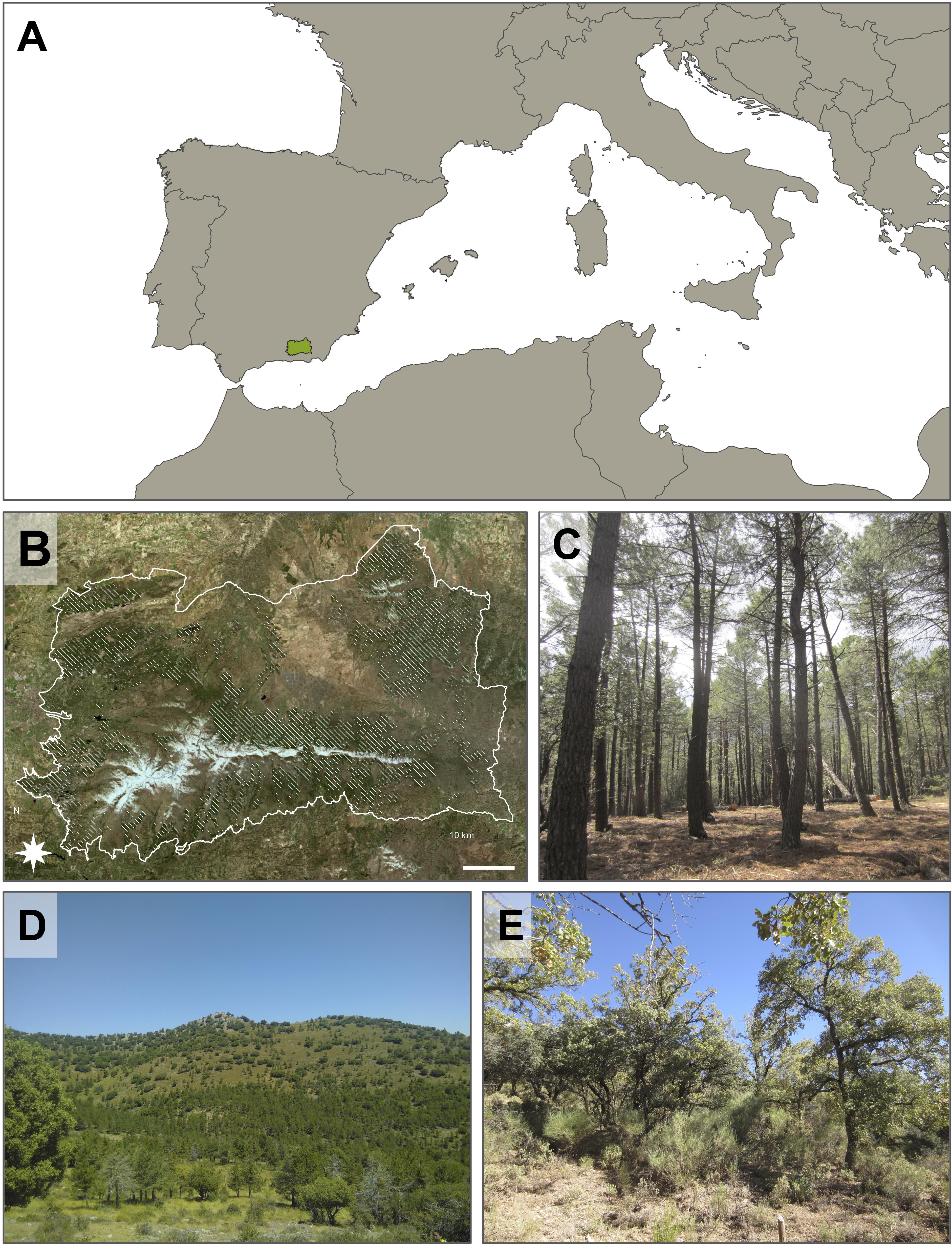
Figure 1. Study area location (A), orthophoto of the study area (B) and pictures of representative forest types: pine plantations (C), mixed open forest (D), oak-dominated stand (E). Shaded area in panel (B) delimitates pine plantations.

Several bioclimatic zones are found within the study area (Rivas Martínez, 1983; REDIAM, 2018). The supramediterranean zone (mean annual temperature 8–13°C) is the one covering most of the area, at low altitudes of Sierra Nevada and connecting with Sierra de Arana. An important proportion of the Sierra de Baza surface is also represented by this bioclimatic zone. Supramediterranean areas are mostly covered by a mosaic of conifer, mixed forests and sclerophyll shrubs. The highest areas represent the oromediterranean zone (mean annual temperature 4–8°C) and are covered by conifers, shrubs and sparse vegetation, except for the very high altitudes in Sierra Nevada, which encompass the cryoromediterranean zone (i.e., alpine tundra, mean annual temperature <4°C). These peaks are covered by scarce vegetation adapted to extreme climatic conditions. The rest of the study area, at altitudes commonly below 1,000 m, is mostly covered by mesomediterranean (mean annual temperature 13–17°C) and thermomediterranean zones (mean annual temperature 17–19°C). The precipitation follows a strong seasonal pattern, with dry summers and precipitation concentrated in a small number of events. Rainfall is the most common form of precipitation. Besides, snowfall at high altitudes is very important since slow melt down and subsequent infiltration into soil increases water availability for plants throughout the spring and summer season. Aspect also determines water availability due to different precipitation evapotranspiration patterns.

The study area is covered by diverse natural vegetation patches in combination with agriculture and Pinus forest plantations. Pine plantations are the dominant land use type, covering around 20% of the study area, with a minor presence of natural pine forests. These plantations were mainly established between the 1950s and 1970s as means to halt soil erosion in recently abandoned agricultural areas. The main species are Maritime pine (Pinus pinaster Aiton), Aleppo pine (Pinus halepensis Miller.), black pine (Pinus nigra Arnold.) and Scotch pine (Pinus sylvestris L.) (Bonet García et al., 2009; Pemán García et al., 2017; Mesa Garrido, 2019). Pines were planted in high densities to drastically reduce soil loss. Afterwards, favourable climate conditions and lack of appropriate post-planting management have resulted in highly dense monospecific even-age stands. As a result, these forest plantations are nowadays under extreme risk by climate change and forest pests, which has resulted in decline and massive mortality processes (Sánchez-Salguero et al., 2010, 2012a).

Almost 40% of the study area is covered with shrublands and abandoned crops with sparse natural vegetation. Some of these areas host sparse trees (mainly Quercus ilex L.), which can be highly relevant seed sources at a local scale. Moreover, in a context of climate change and further abandonment of mountain agriculture activities, these sparsely vegetated systems can be highly important to understand the succession dynamics in pine plantations for two reasons: (1) Due to climate change, currently forested areas could suffer a decline and be replaced by shrublands as these areas become less suitable to sustain high levels of biomass; and (2) Tree species could expand to shrubland areas currently dedicated to marginal activities (mountain agriculture, livestock, fuelwood, and charcoal exploitation, etc.).

Model Initialization

In this section we describe the workflow followed to produce the necessary inputs required by LANDIS-II with PnET-Succession. We first focus on the generation of the initial vegetation conditions, followed by the methodological process to build biophysical inputs. The different sources of information used in this process are listed in Table 1.

TABLE 1

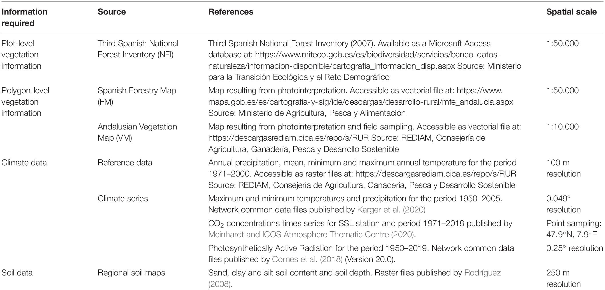
Table 1. Information sources used in this study.

Initial Vegetation Conditions

Most FLMs require estimates of initial conditions in the form of vegetation maps reporting the presence of tree species at the beginning of the simulations. Concretely, LANDIS-II requires a spatial representation of species cohorts by age classes (also called “initial communities”). To generate such vegetation maps, different information sources are often combined following a complex workflow that, if not exhaustively described, is often unreproducible. Even though such workflows can be model- and site-specific, three methodological steps can be defined: (1) Plot-level information (e.g., from national or regional inventories or permanent growth plots) is processed to extract tree measurements such as basal area, age or height; (2) Polygon-level information is processed to select stand-scale, spatially explicit variables which can be linked to plot-level information such as forest type, mean age, canopy cover, etc.; (3) A spatial imputation method is applied to produce a continuous map by assigning plot-level information to polygon-level information. In the following sections, we describe the methodological details for each of the three methodological steps of the workflow, which is summarized in Figure 2.

FIGURE 2

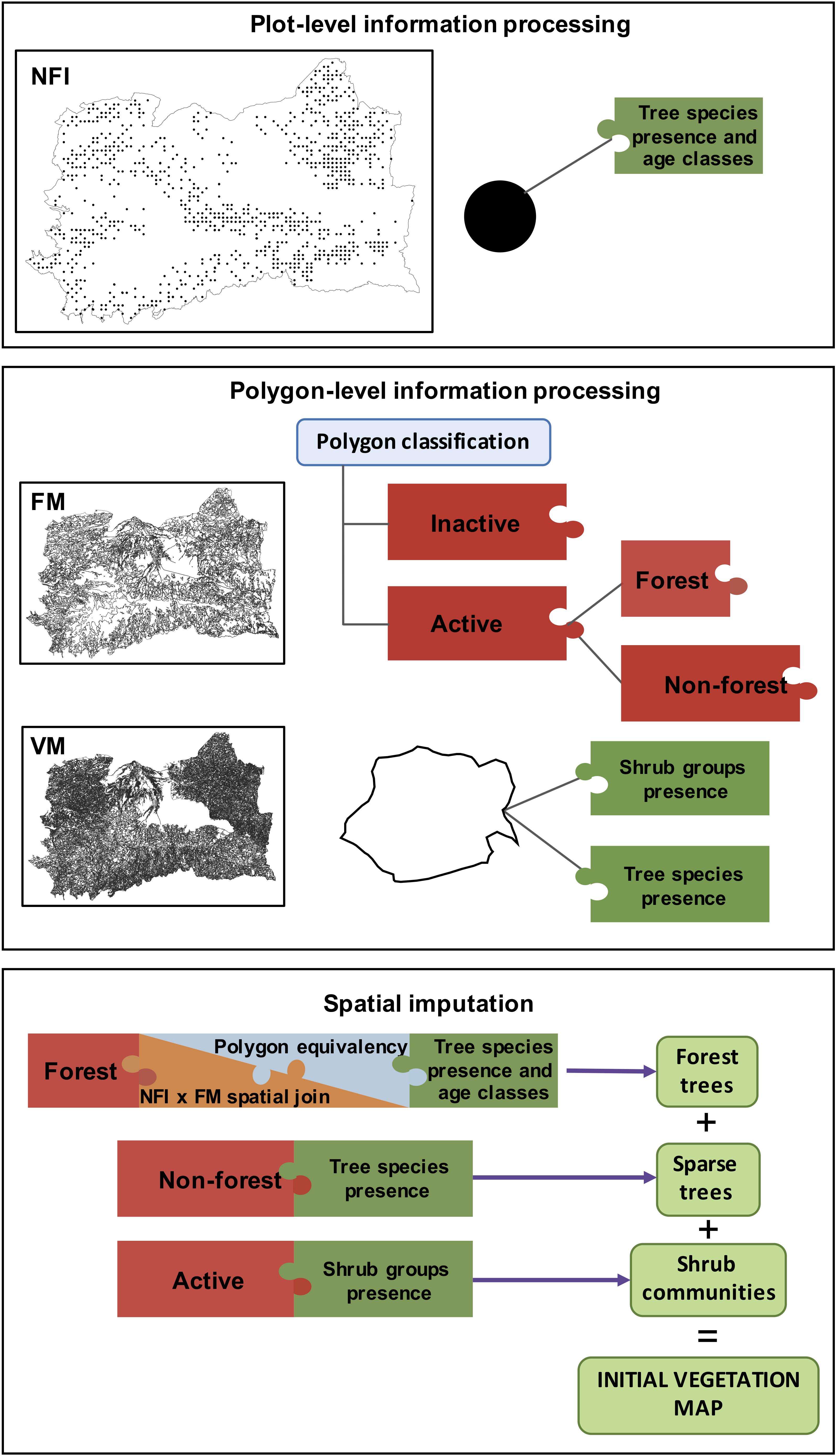
Figure 2. Schematic view describing the workflow of the initial vegetation map generation. Tree species presence and age were extracted from plots of the Third Spanish National Forest Inventory (NFI) during the plot-level information processing phase. During the polygon-level information processing, the Spanish Forestry Map (FM) was used to classify polygons as active/inactive and no forest/forest. The Andalusian Vegetation Map (VM) was used to extract the presence of shrub communities and sparse trees. At the spatial imputation phase, plot- and polygon-level information was combined to generate a continuous map of vegetation.

Plot-level information processing

Plot-level information is necessary to select the most common tree species and some of their demographic features in the area of interest. In our case, the Third Spanish National Forest Inventory (NFI) was used for this purpose (Table 1). The NFI contains homogeneous information about forest covers in Spain by reporting data collected in a systematic network of permanent sampling plots (Alberdi et al., 2017). The plots are evenly distributed on a 1 km² grid throughout the territory and contain plot- and tree-level information for each survey period. In addition to single-tree data (e.g., species, diameter, height, form, and health status), the plot is described in terms of the three most dominant tree species contributing to canopy cover. We selected the tree species to include in the model simulations based on the total coverage value of the species within the study area.

Tree age is often not available at single-tree level and its estimation is challenging as several factors influence growth rate of individual trees, leading to very different tree characteristics for the same age. Nevertheless, LANDIS-II uses cohort age-classes as a proxy for biomass, and therefore an estimated age is required for each species across the landscape. NFI provides estimated stand age for plots within even-aged stands. In our area, even-aged stands are composed by Pinus spp. Since these plots also have associated individual tree measurements (e.g., diameter, height), we calculated the average diameter per species and plot and joined it to the assigned stand age. In order to have as many observations as possible, we expanded the considered dataset to all plots within even-age stands from surrounding regions (provinces of Granada and Almeria). Since no estimated age was available for plots within uneven-age stands (mainly Quercus spp. and Populus nigra), a semi-quantitative method was applied. We used yield tables available from the literature (Teobaldelli et al., 2010). Then, we generated an age assignment table containing correspondence rules between tree age, diameter and height for each species under consideration. This table was validated based on expertise and observations in the study area. Finally, the age assignment table was used to attribute an age class to the species in each NFI plot (see Supplementary Table 1 for more details).

Polygon-level information processing

Many government and private forestry organizations utilize cartographic products to support forest management. Polygon-level information usually contains forest variables at a landscape scale such as forest type, coverage or stand development stage. Here, we used the Spanish Forestry Map (FM) and the Andalusian Vegetation Map (VM) as the main source of spatially explicit landscape information (Table 1). The FM is a vectorial file generated by photointerpretation. It contains a series of attributes describing the forest vegetation for each polygon: polygon identifiers and surface; province and region; forest and land use characteristics (vegetation type, structural type, land use categories); name, coverage and state of the three most dominant species in dominance order; and tree and total coverage fraction. Based on these attributes, polygons were classified as active (those containing or potentially containing vegetation units useful for our purpose) or inactive (those where natural succession is hampered by human activities: crops, infrastructures, firebreaks, etc.). Active polygons were in turn classified as forest and non-forest. Forest polygons have an average size of 51 ha and a maximum of 357 ha.

The VM is also a vectorial file that contains an extensive list of attributes (140) describing the presence and characteristics of the tree species, shrubs and pastures present in each polygon (e.g., vegetation community, canopy coverage) at a higher resolution than the FM. Due to the importance of sparse trees and shrublands in our study area (see section “Study Area”), we used the VM to consider the occurrence of sparse trees in non-forest polygons in the initial vegetation map. Moreover, since the VM also provides information about shrubs, grasslands and pastures, we used a variable termed “life form” attribute to analyse the presence of shrubs within the study area. The life form attribute is based on the classification proposed by Raunkiaer (1934) and subsequently revised by Ellenberg and Mueller-Dombois (1967). According to this classification, plants can be: microphanerophytes (“evergreen perennial plants that grow between 2 and 5 m, or whose shoots do not die back periodically to that height limit”), nanophanerophytes (“evergreen perennial plants that grow below 2 m tall, or whose shoots do not die back periodically to that height limit”), chamaephytes (“evergreen perennial plants whose mature branch or shoot system remains perennially within 25–50 cm above ground surface, or plants that grow taller than 25–50 cm, but whose shoots die back periodically to that height limit”), hemicryptophytes (“perennial plants with periodic shoot reduction to a remnant shoot system that lies relatively flat on the ground surface”), geophytes (“perennial plants with periodic reduction of the complete shoot system to storage organs that are imbedded in the soil”), therophytes (“annual plants whose shoot and root system dies after seed production and which complete their whole life cycle within 1 year”). Shrub communities’ size was extracted from this classification. Hemicryptophytes, geophytes and therophytes life forms were not considered for the analysis as they mostly refer to species with short life cycles. As a result, the presence of tall (2–5 m), medium (0.5–2 m), short (<0.5 m) shrub communities was extracted for each polygon in the study area. Each of these shrub communities was parameterized individually in PnET-Succession (see details below).

Spatial imputation

Spatial imputation is applied to combine plot-level to polygon-level information. To generate the initial vegetation map suitable for LANDIS-II, we combined plot- and tree-level information (NFI) with polygon-level information (FM and VM). The final aim of this step is to produce a forest composition map containing the species-age assemblage (species and age of each cohort) in every cell within the study area (see Duveneck et al., 2015 for the description of a similar approach in North America).

First, we performed a spatial join between the forest polygons from the FM and the plots from the NFI (Figure 2). FM polygons containing one single NFI plot were assigned the species-age assemblage of the surveyed plot. FM polygons with more than one NFI plot were assigned the species-age assemblage which results from merging all plots species-age assemblages. This only occurred in a small proportion of cases: 80 out of 789 forest polygons had two NFI plots in them, 3 polygons had 3 NFI plots in them and one polygon had 4 plots in it.

Forestry Map polygons without NFI plots were analysed to identify an equivalent polygon among those which have one or more intersecting NFI plots. Polygon equivalency was analysed at three levels: (i) Full equivalency: polygons matching vegetation type, species dominance, species development state, and total coverage fraction; (ii) Partial equivalency: polygons matching vegetation type, species dominance, and total coverage fraction; and (iii) Species equivalency: polygons matching species dominance and total coverage fraction. FM polygons were assigned the species-age assemblage of their equivalent polygon. If there were more than one equivalent polygon, the polygon was assigned the species-age assemblage resulting from the merge of all possible ones. FM polygons with no equivalent polygons were further analysed based on their species composition, without considering species dominance order. These polygons were assigned the species-age assemblage corresponding to the most common species-age assemblage containing the same species as the considered polygon in the whole study area. FM polygons containing species assemblages not occurring in the previously analysed polygons were assigned one cohort of each of the species present in it. The age of this cohort corresponded to the most common age for each species among all previously analysed polygons. This procedure resulted in the description of the forest trees within the study area.

Second, polygons labelled as non-forest by FM, were imputed to include sparse trees (Figure 2). We used VM to gather information for those polygons. Since VM does not report any variable describing the age of the species, VM polygons were imputed a species-age assemblage containing the reported species with the most common age for that species in the rest of the study area. By doing so, the description of the sparse trees within the study area was completed.

Third, we imputed shrub communities within the landscape by assigning the corresponding shrub community-age assemblage to each VM polygon (Figure 2). Shrubs were not allocated to different age classes but instead we arbitrarily assigned age 10 for all polygons. Since in LANDIS-II shrub biomass should not exceed tree biomass (see section “Model Description”), the role of shrubs in the model is mainly to compete for light and water in the understory (e.g., affecting establishment), thus we believe age class assignation for shrubs was not necessary.

Finally, we obtained the initial vegetation map by combining forest trees, sparse trees and shrubs communities. The map was rasterized at 100 m resolution (1 ha cells). Each cell was labelled with a code associated to a list of unique species-cohort assemblages.

Biophysical Inputs

The FLM LANDIS-II requires an input map of ecoregions as biophysical inputs. LANDIS-II ecoregions are continuous or discontinuous areas of the landscape which share climate conditions and soil texture (see section “Model Description”). To generate the map of ecoregions, we used a reference climate dataset and a regional soil map (Table 1). The reference climate dataset reports annual precipitation and mean, minimum and maximum temperature for the period 1971–2000 at a 100 m resolution. Firstly, an unsupervised k-means clustering was applied to the climate dataset to lump together cells with similar climate. MacQueen algorithm was used in this clustering (MacQueen, 1967). We evaluated different numbers of clusters and eventually ended up with four climate regions. The resulting ecoregions agree with our expectations considering topography and the bioclimatic zones found in the study area (Figure 3).

FIGURE 3

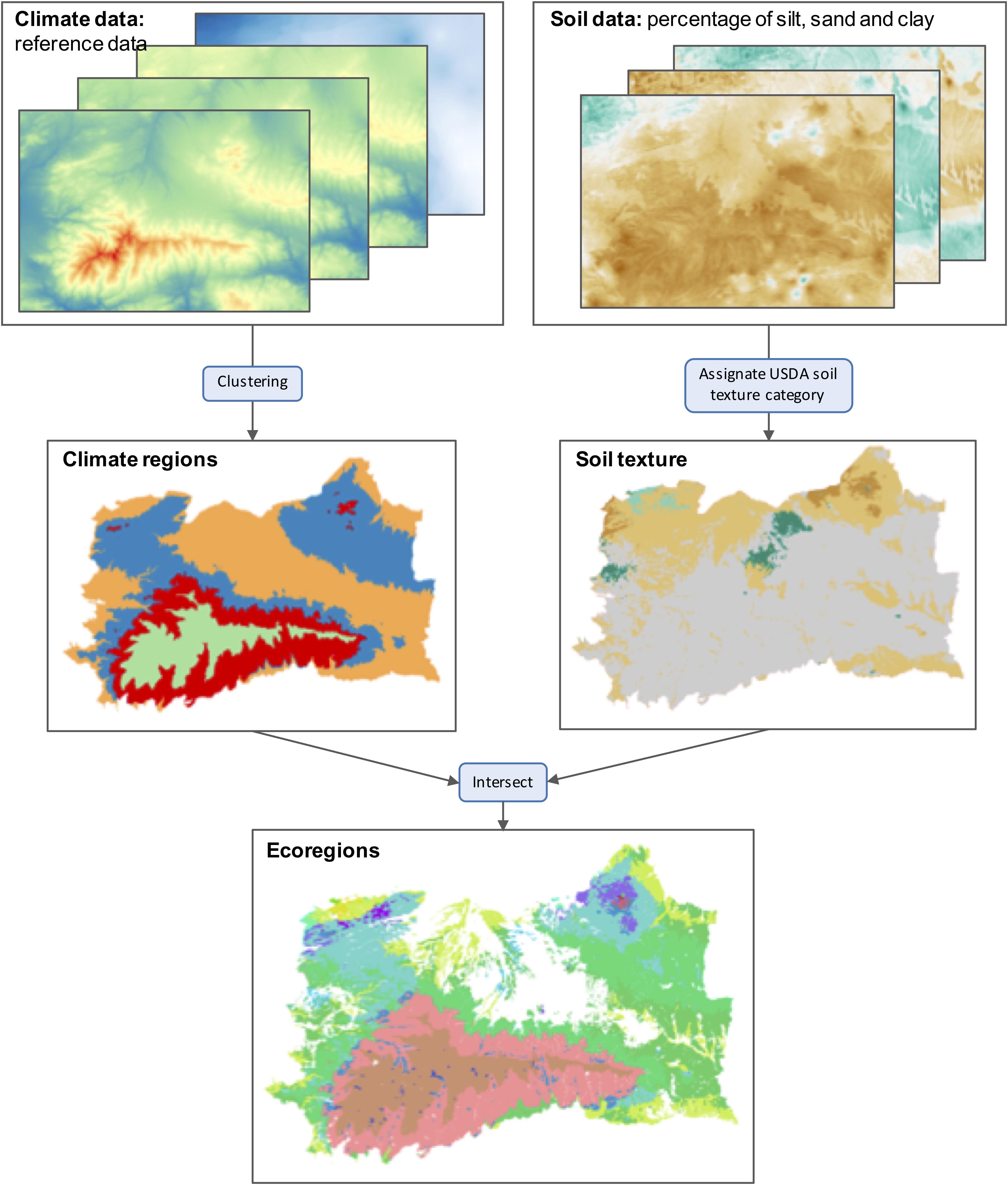
Figure 3. Schematic view of workflow followed to produce the ecoregions map. Reference climate data consist of annual precipitation, mean, minimum and maximum annual temperature for the period 1971–2000 at 100 m resolution. Clustering of climate data resulted in four climate regions. Soil data consist of a percentage of silt, sand and clay at 250 m resolution. The intersection of climate regions and soil textures resulted in 27 ecoregions.

The resulting climate regions map was intersected with the soil texture map. The soil map reports the percentage of sand, silt and clay at a 250 m resolution. This map was derived by simply translating the percentages of sand, silt and clay to USDA soil texture categories. The final ecoregions map was therefore produced by overlapping the climate regions and the soil textures maps. This resulted in a total of 28 unique ecoregions defined by both a climate region and a soil type (Figure 3).

PnET-Succession also requires rooting depth for each ecoregion. Ecoregion rooting depth was calculated based on soil depth classes reported in the soil map (0–250 mm, 250–500 mm, 500–1,000 mm, 1,000–1,500 mm, >1,500 mm). The midpoint of each class was used to calculate the most frequent rooting depth for each ecoregion. Precipitation Loss Fraction and Leakage Fraction were given values of 0.6 and 1 for all ecoregions. All other PnET-Succession ecoregions parameters were given default values. A complete dataset containing model inputs is provided (see section “Data availability”).

Calibration of Model Parameters

LANDIS-II and PnET-Succession require a set of parameter values for each species simulated in the landscape. Generic species parameters are required irrespective of the chosen succession extension (e.g., longevity, sexual maturity), while others are required by PnET-Succession (e.g., foliage nitrogen, foliage turnover, minimal, and optimal photosynthetic temperature). We firstly defined an initial set of parameter values from multiple sources. Then, we ran single-cell simulations to verify the species behaviour (e.g., growth, photosynthetic rates) under different conditions. On a single, empty 100 m cell, a single 10-years old cohort of each species was initialized and grown for 200 years preventing establishment of new cohorts. Five replicates were run for each simulation using static monthly averages of temperature, precipitation, PAR and CO₂ (Table 1 and Supplementary Figures 4–6). Baseline climate conditions were used to avoid introducing variability due to fluctuating climate (Gustafson and Miranda, 2019).

The results of these simulations were compared with species biomass estimations for the study area and literature information. Biomass estimations were calculated for P. halepensis, P. nigra, P. pinaster, P. sylvestris, Q. ilex, and Q. pyrenaica based on forest inventory data and allometric equations published in Montero et al. (2005). Simulated versus observed Relative Growth Rates in relation to species biomass were used for comparison as this metric is independent from age, which has a high uncertainty degree in NFI data.

Following calibration guidelines for PnET-Succession (De Bruijn et al., 2014; Gustafson and Miranda, 2019) and evidences from a sensitivity analysis with the same model (McKenzie et al., 2019), we adjusted the most influential species-specific parameter values in an iterative process until the species showed the expected behaviour based on authors’ expertise and observations.

We also evaluated the response of competing assemblages of species typical of the different forest types included in our landscape. These multi-species simulations allow the calibration in relative terms, as well-known competition effects can be assessed and species parameters can be adjusted accordingly. In these simulations, species are established in the cell at the same time and no new establishment is allowed, which is often not the case in natural ecosystems. Thus, the observed species development is the result of their growth traits and their different performance under competition and not due to different establishment strategies or other advantages.

Landscape Simulation

We simulated forest dynamics at the landscape scale incorporating the effect of spatial processes such as dispersal and climate and soil heterogeneity. We initialized the model with the biophysical inputs described above and with the parameters calibrated in the previous step. To verify the influence of shrub communities on simulated forest dynamics, we initialized LANDIS-II with two different vegetation datasets: (1) With shrub communities and (2) Without shrub communities. Since the aim of this study was to initialize the landscape for further experiments with LANDIS-II and PnET-Succession, neither natural nor human-driven disturbances (i.e., fire, harvest) were included in the experiment. We ran five model replicates using baseline climate for 200 years (Table 1 and Supplementary Figures 4–6). We analysed model outputs in terms of temporal patterns of average biomass for each species. Moreover, we mapped and compared total aboveground biomass for selected simulation years across the landscape. All analyses were performed in R version 3.5.3 (R Core Team, 2020) and QGIS 3.10 (QGIS Development Team, 2020).

Results

Spatial Imputation and Initial Vegetation Map

The analysis of 981 NFI plots falling within the study area resulted in eight species having a coverage value higher than 1%: Quercus ilex (25%), Pinus sylvestris (18%), Pinus pinaster (16%), Pinus nigra (16%), Pinus halepensis (16%), Quercus pyrenaica (2%), Populus nigra (1%), and Juniperus oxycedrus (1%). These species were selected to be included in the study. Besides, two extra species—Quercus faginea and Juniperus communis—were also included due to their importance in specific environments. J. communis covers vast areas above the tree line (cushion shape shrubs) (García, 2001) and Q. faginea is also locally abundant.

The analysis of the FM resulted in a classification of active versus inactive cells within the study area. Inactive areas cover 19% of the study area and mainly refer to crops and firebreaks (17.3%). Moreover, active cells were classified as forest and non-forest, which represent 41 and 40% of the study area, respectively.

The intersection of NFI plots and FM polygons defined the species-age assemblage of a total of 789 polygons within the study area. Out of 3,113 polygons with no NFI plot in them, 84% of them were imputed based on equivalent polygons (55% full equivalent, 22% partial equivalent and 7% species equivalent). The remaining 16% of polygons were imputed the species assemblage reported in the FM and the most common age for each of the species.

The use of the VM allowed a more detailed description of active non-forest areas. The analysis of sparse trees in non-forest polygons increased by 4% the surface of the study area where tree species are present. Even though it may seem as a small portion of the landscape, these sparse trees can represent important seed sources when long-term forest dynamics are simulated. Moreover, the VM analysis allowed the inclusion of shrub communities in the landscape’s cells, which can affect the shade conditions as well as water availability.

Figure 4 shows the initial vegetation map as a result of combining the presence of forest trees, sparse trees and shrubs communities. Several portions of the landscape are covered by shrublands and Juniperus spp., surrounded by a mosaic of Pinus spp., Quercus spp. and mixed Pinus-Quercus forests, with a minor presence of Populus nigra.

FIGURE 4

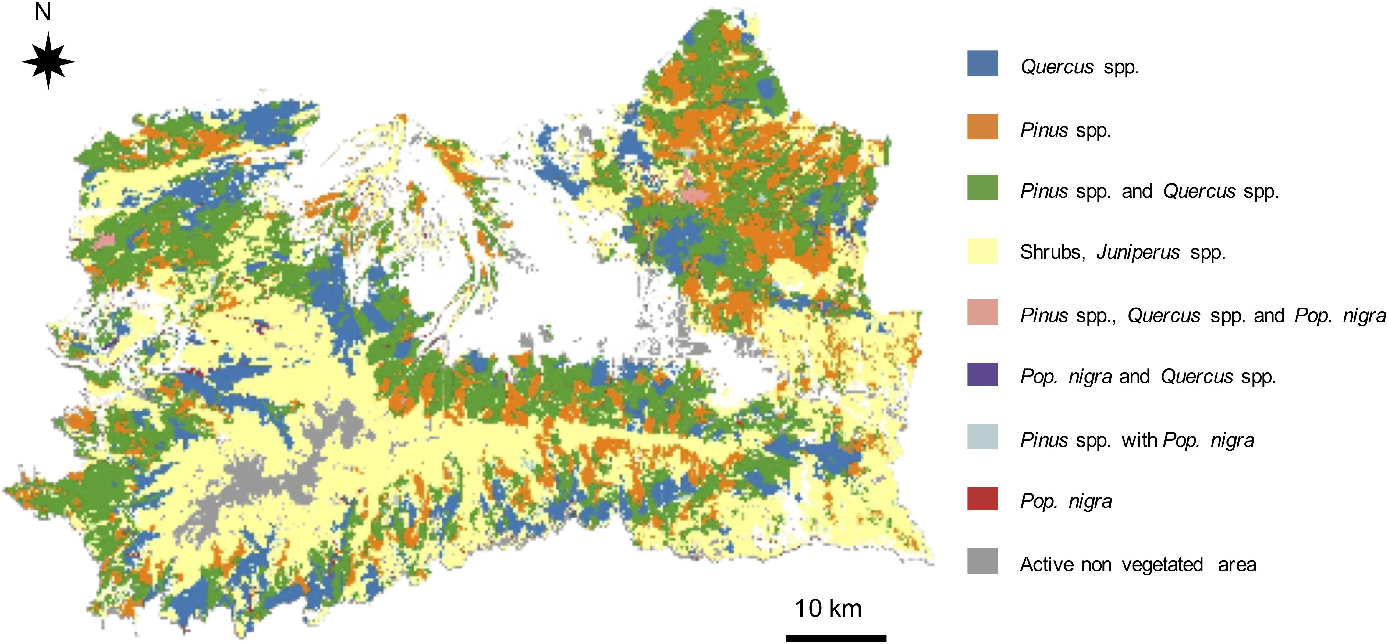
Figure 4. Map of initial vegetation conditions including shrub communities. Each category represents a community dominated by one or more tree species, where shrubs and Juniperus spp. may also be present.

Calibration of Model Parameters by Means of Site-Level Simulations

Estimating species parameter values was a complex task due to the amount of information sources required to cover all of them. Table 2 reports the most important parameters required by LANDIS-II and PnET-Succession. A detailed explanation of all parameter values, sources and rationales for their adoption is provided in Supplementary Table 2.

TABLE 2

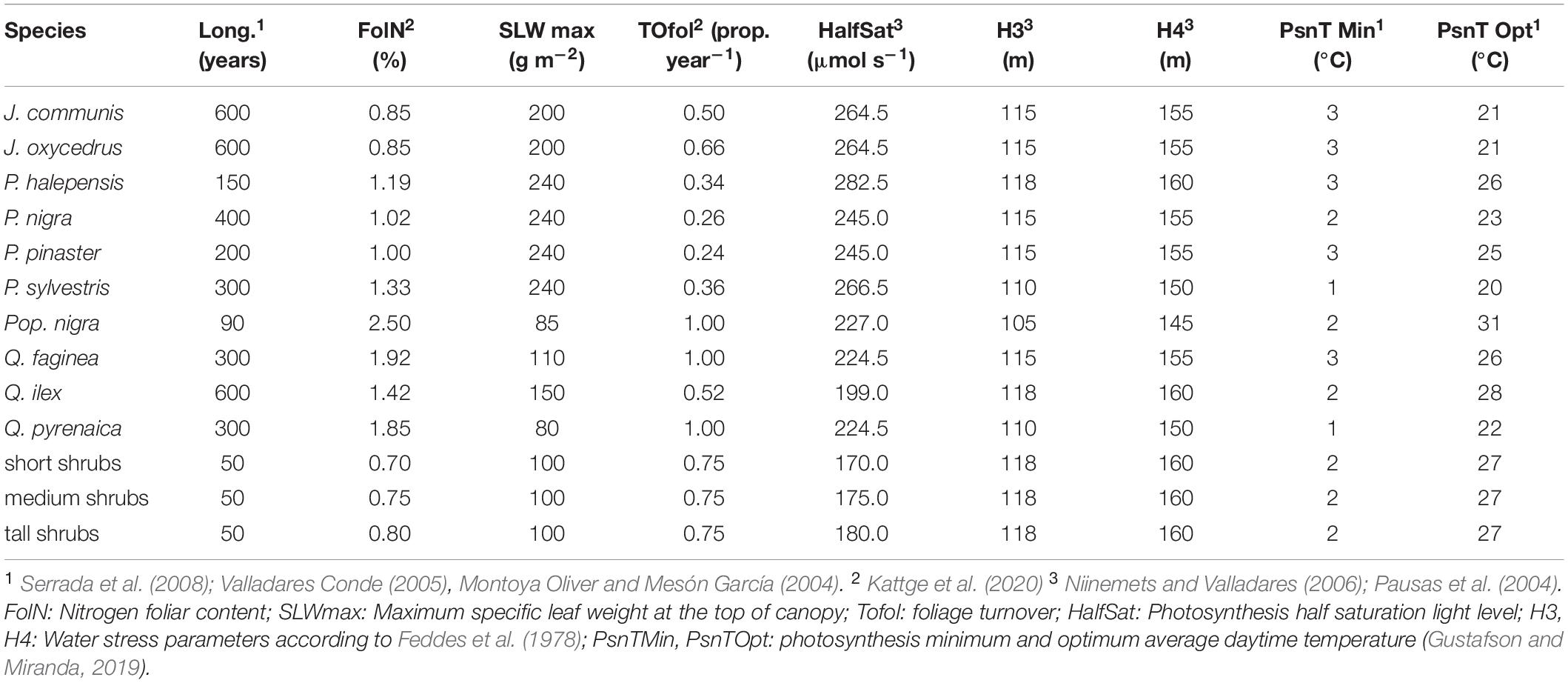
Table 2. Species parameter values for LANDIS-II and PnET-Succession.

Biomass estimations for P. halepensis, P. nigra, P. pinaster, P. sylvestris, Q. ilex, and Q. pyrenaica were compared with results from single-cell simulations initialized with individual species. Results of biomass and photosynthetic rates of species simulated individually on a single cell are reported in the Supplementary Figures 1–3. Simulated results are within the range of estimations, although estimations are highly variable among plots.

Among the more than 70 of single-cell simulations that were performed, we chose to show here two representing typical species assemblages of low and high altitude forest types (Figure 5). In the low altitude forest type, composed of two pine and two oak species, our results indicated a dominance of Q. ilex over Q. faginea, P. halepensis, and P. pinaster (Figure 5A). Cohorts of the two latter species were simulated to die by year 140 and 190, respectively, since they approached their longevity (pink and blue lines). Q. ilex clearly dominated Q. faginea but it did not fully outcompete it. The advantage of Q. ilex in this forest community seems to be related to its capacity to start photosynthesizing earlier in spring than the other species (Figure 5B).

FIGURE 5

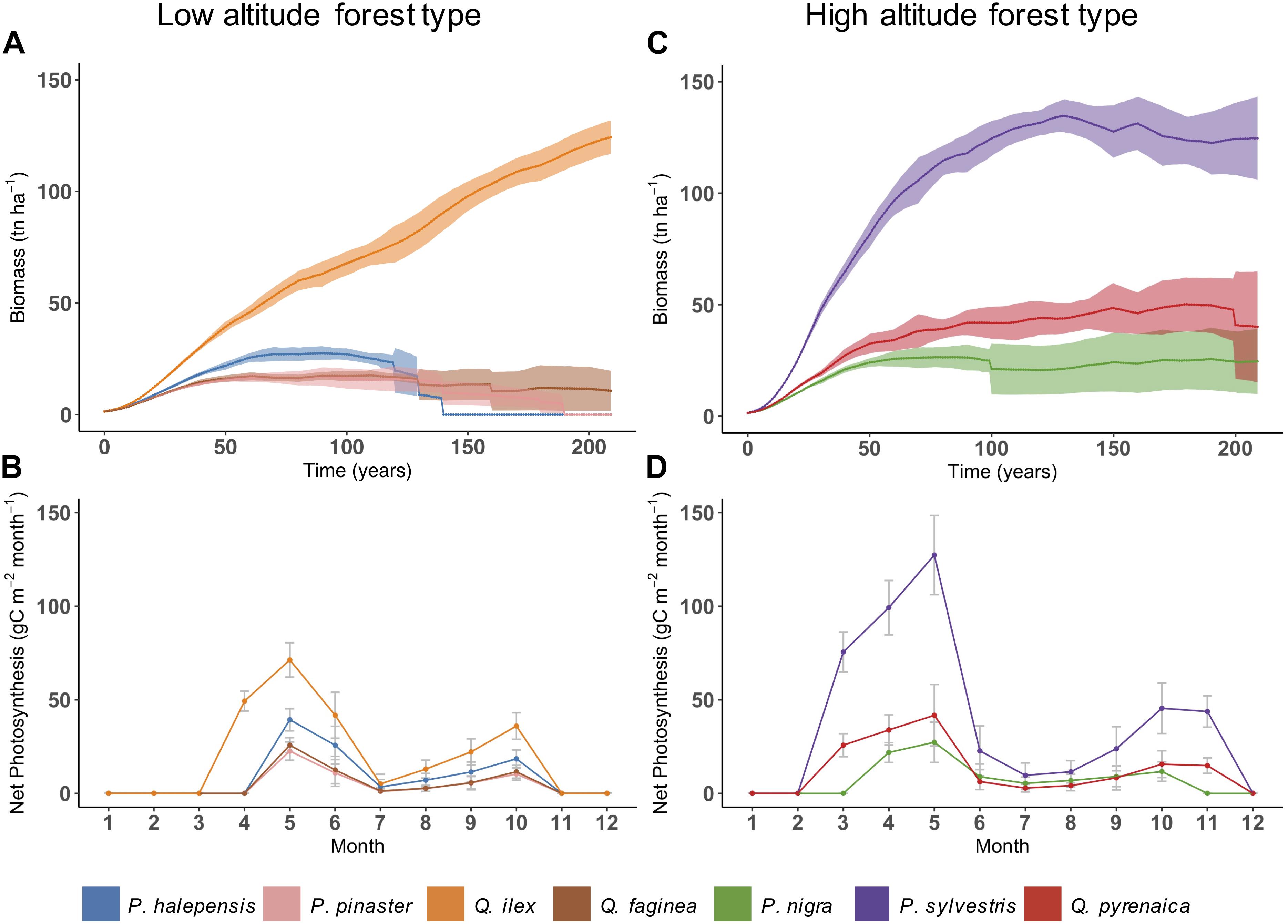
Figure 5. Mean simulated annual total biomass (wood, roots and foliage) (A,C) and monthly net photosynthesis (B,D) for the two chosen forest types. Shaded area refers to standard deviation. Values of net photosynthesis are averages between years 50–75, with error bars indicating standard deviation. Note that lines connecting the points serve for illustrative purposes only, since PnET-Succession simulates photosynthesis at monthly time scale (not daily).

In the high altitude forest type, P. sylvestris, P. nigra, and Q. pyrenaica coexisted along the simulation, although P. sylvestris built higher biomass compared to the other two species (Figure 5C). The advantage of P. sylvestris was related to its higher photosynthetic rate from the beginning of the season, while Q. pyrenaica, being a deciduous species, increased its photosynthesis more gradually after having built foliage biomass (Figure 5D). Generally, we found that PnET-Succession reproduced reasonably well the bimodal growth patterns of Mediterranean tree species, mostly occurring during spring and fall instead of summer which is characterized by a lack of precipitations.

Landscape-Level Simulation

Both simulations with and without shrubs showed a trend to increase the average biomass of all tree species during the first years of the simulation and stabilization afterwards (Figure 6). In the simulation including shrubs, this increase was slower than in the simulation without shrubs, with a faster increase in the first 50 years. In both simulations the total average biomass at stabilization was around 100 tn ha^–1.

FIGURE 6

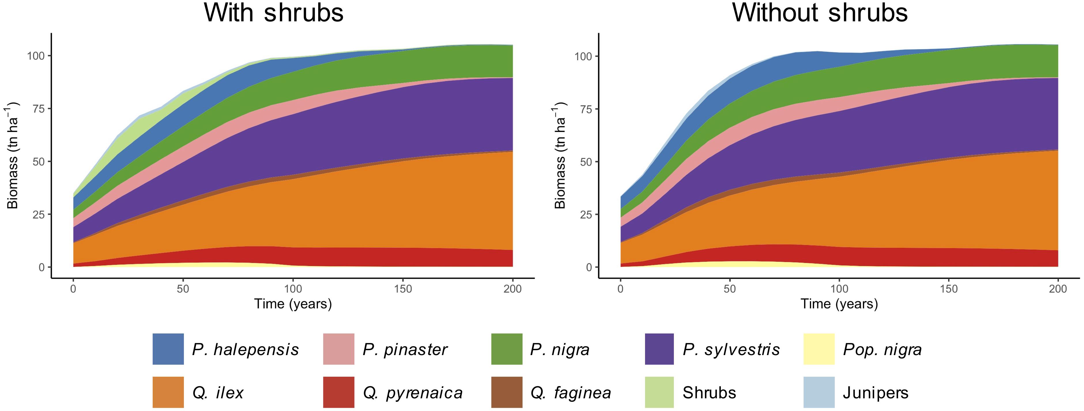
Figure 6. Average biomass of species through time for the whole landscape. Note that Junipers (J. communis and J. oxycedrus) and shrub communities (short, medium, and tall) have been grouped together.

We found differences among species in terms of simulated biomass growth. Among pine species, P. sylvestris and P. nigra were those with a higher increase of average biomass in both simulations. Biomass of P. halepensis and P. pinaster increased during the first 50 years, followed by a decline and disappearance from the landscape toward the last decades of the simulation. Among oaks, biomass of Q. ilex increased notably, while Q. pyrenaica increased at lower rates and stabilized after about 100 years. Biomass of Q. faginea and Pop. nigra had similar trends, increasing slightly in the early years and declining afterwards, but still maintaining presence at low levels of biomass. Junipers slightly increased their biomass during the first 30 years and then strongly declined. These species show similar patterns in both simulations, but under the simulation without shrubs we observe a steeper increase of biomass during the first years. Shrub communities increased their average biomass during the first 40 years and declined afterwards.

Initial total landscape biomass (time 0) was similar in both simulations since shrub communities accounted for low levels of biomass (5.1% of total biomass). At time 50, the area with high biomass is wider in the simulation without shrubs (Figure 7). This pattern was observed at time 100 too, although the difference between the two simulations was smaller (see total biomass at each time step in Figure 7). At time 150 and 200, both simulations showed a similar quantity and distribution of the biomass across the landscape, with slightly higher values of biomass in the simulation without shrubs than in the one with shrubs. The biomass distribution within the study area followed the altitudinal gradient, with higher biomass found at medium elevations, specially at time step 150. At the beginning of the simulation, areas at high elevation (above c.a 2,000 m a.s.l.) show the smallest values of biomass relatively to the rest of the study area. This pattern remained by the end of the simulation in both cases.

FIGURE 7

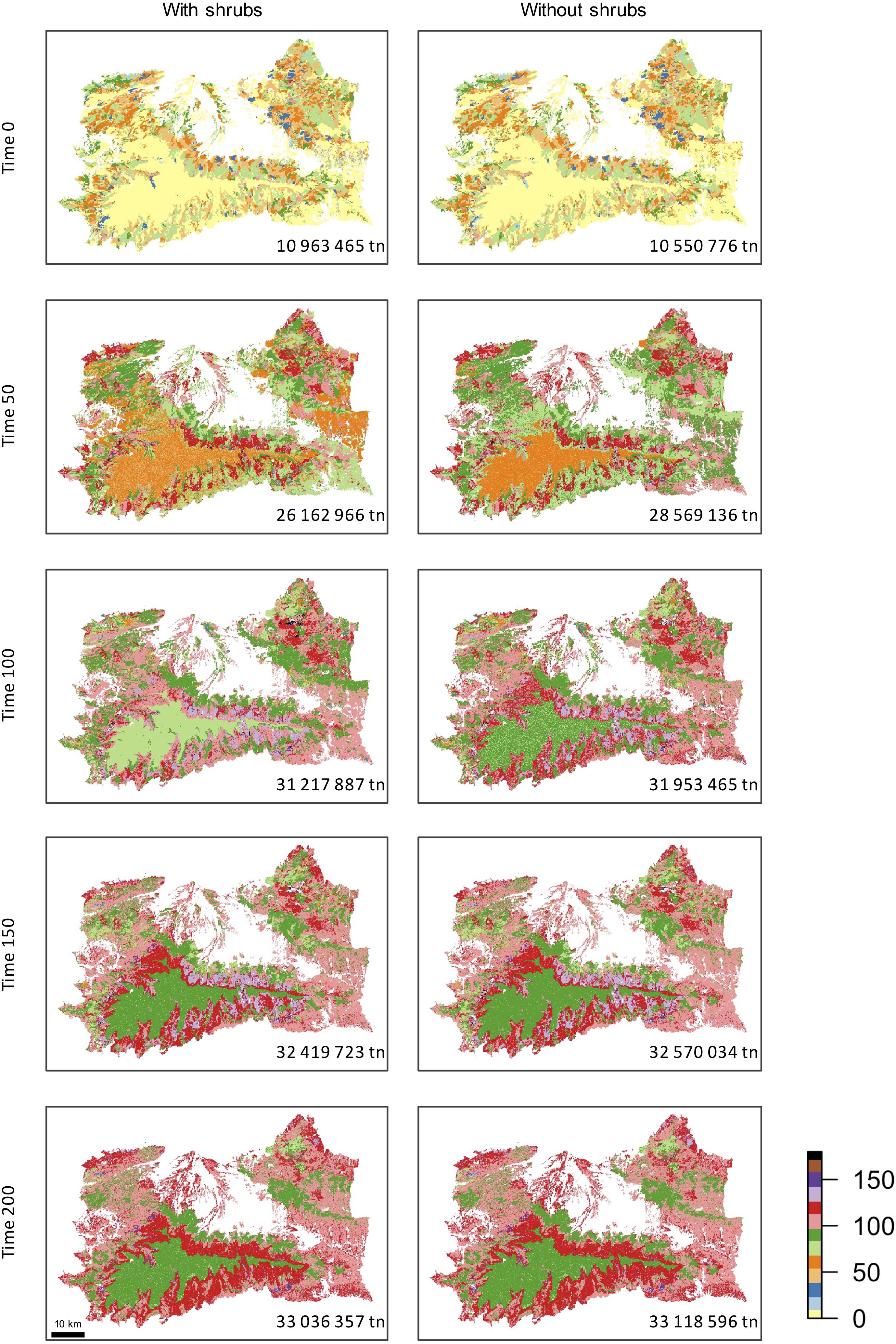
Figure 7. Total aboveground biomass (tn ha-1) at years 0, 50, 100, 150, and 200 for the two simulations, as indicated in the scale bar on the right. Number in each panel indicates the total aboveground biomass (Tg) for the whole landscape at each time step.

Discussion

We provide detailed step-by-step example to initialize, calibrate and set up a forest landscape model. Our work could help other potential users to better understand what is required to start applying such models. Thus, our fully documented methodological process represents a step forward toward the transparent application of forest landscape models in regions without prior application. We also made available a high-resolution map of vegetation conditions and calibration details for a large mountainous landscape in the European Mediterranean area, together with the input data and scripts used in the process. Our landscape level simulations reveal distinct dynamics among species according to their competitive potential and simulated intra-annual growth. These results also indicate that shrub communities shall be considered in forest landscape models as they have the potential to influence forest dynamics by delaying growth and expansion of tree species in Mediterranean ecosystems.

Spatial Imputation and Initial Vegetation Conditions

The selection of species to be included in modelling studies is typically done by analysing data from terrestrial plot measurements such as forest inventories (e.g., Wang et al., 2019). However, for certain ecosystems, limiting this inspection to forest inventories has some disadvantages. Forest inventory data commonly report information on tree species, neglecting important functional groups (in our case, J. communis and shrubs communities). Moreover, selection is usually based on variables such as basal area or stand coverage. This selection may result in the exclusion of species that may not be abundant at the landscape level but whose presence is crucial at the local scale. For example, Q. faginea would have been initially excluded from our study since its coverage falls below the 1% of the study area (0.03%). However, this species is found at high abundance in some locations and has a higher susceptibility to summer drought than Q. ilex. Therefore, the dynamics and distribution of Q. faginea are expected to be highly affected by climate change (Quero et al., 2006). Similarly, J. communis was included due to its importance in areas above the treeline. In these areas, J. communis is susceptible to interact with tree species under climate change conditions by limiting or facilitating uphill migration of tree species. Therefore, even though forest inventory data are important resources for generating inputs for FLMs, we recommend combining such datasets with other information sources (e.g., vegetation maps, local studies) according to the forest ecosystem under consideration and study focus—in our case, climate change applications—. Considering factors such as relevance in specific habitats or cultural importance (e.g., Lucash et al., 2019) may result in inclusion or exclusion of some species.

Our method, which combined multiple information sources allows the inclusion of fine-coarse information such as the presence of sparse trees and shrub communities. The inclusion of sparse trees in the initial vegetation map is important in the Mediterranean mountains, since we simulate succession in pine plantations, artificially created stands where regeneration is highly affected by seed dispersal from adjacent patches of native vegetation (González-Moreno et al., 2011; Navarro-González et al., 2013). Although shrubs’ biomass is generally low, they can shade the forest floor and therefore influence simulated light and soil water dynamics, as well as affect establishment (further discussion below). Moreover, shrubs play a key role in other processes such as fire dynamics due to their role as fuel in forest fires (Syphard et al., 2006).

In this study, we have used a categorical methodology for the spatial imputation, contrary to commonly used methods based on geographic or data space distance (e.g., Wilson et al., 2012; Ohmann et al., 2014; Duveneck et al., 2015). Our study area is a highly anthropized mosaic of different land uses and management regimes, and therefore imputation based solely on distance might not have been an appropriate criterion, as indicated by Duveneck et al. (2015). For example, the most common forest type in our landscape, pine plantations, are the result of past forestry policies which were applied almost simultaneously all over the region. Therefore, a high similarity is expected between stands, regardless of the physical distance between them. This is a common situation in other Mediterranean ecosystems (European Environmental Agency [EEA], 2016), and therefore this approach could also be used in such cases.

The uncertainties of this methodology are inherently related to the uncertainties of the information sources. Besides, an additional source of uncertainty in the initial vegetation conditions map is related to the assignation of age to cohorts. Tree age data is rarely available at single-tree level in forest datasets, as reliable tree age estimations are resource-consuming and often invasive (Fazan et al., 2012; Rohner et al., 2013). Thus, modellers are commonly forced to assign each tree (or cohort) to an age class inferring it from available measurements (e.g., diameter, height, average stand age; Abrams, 1985; Rozas, 2003). In the case of LANDIS-II, a cohort’s age determines simulated biomass, which in turn influences light and water availability at cell-level. Therefore, assumptions in the age assignation process may not be so relevant as long as the relative difference between species reflects real conditions. Considering this, we created correspondence rules between tree age and diameter and height for each of the simulated species and age classes. Thus, the growth pattern assigned to each of the species is relative to the other species, reflecting the differential access to water and light by each species-age. This methodology could be further improved by considering additional local yield tables and observations. Nevertheless, by documenting such correspondence rules the model inputs generation is significantly more transparent and reproducible than other LANDIS-II studies (e.g., Mina et al., 2021).

Our goal was to increase the reproducibility of model input generation by ensuring high transparency and detail in the process description. The methodology presented in this study does not necessarily introduce new methods compared to previous studies (e.g., He et al., 1998) but rather it highlights all aspects of the process, which we believe could be of great benefit for beginner modellers to set up applications in new landscapes. Firstly, considering multiple information sources at plot- and polygon-level may be necessary. In our case, multiple vegetation maps were required to consider forested areas, dispersed trees and shrub communities. Secondly, the collected information likely requires processing and transformation, which may introduce assumptions (e.g., age assignation). Thirdly, the selection of the appropriate spatial imputation method should consider the study area characteristics (e.g., coetaneous patches of pine plantations) and available information.

Calibration of Model Parameters and Site-Level Simulations

Calibration of model parameters was performed by running simulations and testing long-term species dynamics and competitive interactions at site-level. The obtained results were iteratively assessed to adjust parameter values until the species showed their expected growing patterns. Experiments at site scale using landscape models have also been used before to analyse the influence of different factors on model outputs by avoiding the high complexity resulting from large landscapes simulations (Gustafson et al., 2017, 2018).

During the calibration phase, species parameters were adjusted to ensure that the model simulates realistic species biomass estimations. Species biomass data derived from field observations (e.g., growth-and-yield sites, inventories and permanent plots) are usually highly variable as they differ depending on multiple factors (e.g., location, stand development, site index). Moreover, biomass values often have a high degree of uncertainty, since they are commonly estimated based on general allometric equations from other measured variables (e.g., diameter, height, wood density) (Forrester et al., 2017). Therefore, such comparisons should be interpreted with caution. In this study we used such estimations to ensure that the simulated biomass falls within realistic ranges rather than adjusting parameter values to match the exact values (see Supplementary Figure 3). With this approach, we calibrated the most relevant species for this study (P. halepensis, P. nigra, P. pinaster, P. sylvestris, Q. ilex, and Q. pyrenaica).

Besides, we review here other studies which provide biomass estimations for some of our species. The dynamics of Q. pyrenaica stands have been studied by Santa Regina (2000), who estimated its biomass in four plots in north-western Spain. Our simulations have a high degree of agreement for foliage biomass, while certain overestimation remains for wood biomass. This difference, nevertheless, can be justified as in the plots studied by Santa Regina (2000) the presence of shrubs could be reducing Q. pyrenaica productivity. Río and Sterba (2009) studied the productivity of mixed stands of P. sylvestris and Q. pyrenaica. They found that although P. sylvestris is less productive when growing in mixed stands, the reduction in productivity is smaller than the reduction in occupied area. Accordingly, our simulations show a decrease in productivity of P. sylvestris when growing together with other species such as Q. pyrenaica, but it remains as a highly productive species.

Other methodologies have been applied for model calibration (e.g., Duveneck et al., 2017; Cassell et al., 2019; Mina et al., 2021). As an example, Duveneck et al. (2017) used data from flux towers within New England (United States) to calibrate PnET parameters. The application of some methodologies over others usually responds to the availability of data for the simulated area. In this sense, the lack of available biomass accumulation curves limited the application of more exhaustive calibration methodologies. Our calibration could therefore be improved if additional data sets become available, such as high-resolution biomass measurements or growth rates based on flux towers measurements.

Our results clearly show that PnET-Succession reproduces the characteristic bimodal growth observed in Mediterranean species (Larcher, 2000). This growth pattern is the result of dry summer conditions, which impose a limitation for growth to numerous species. Thus, Mediterranean species often show two peaks of productivity through the year, in late spring and fall (Camarero et al., 2010; Gutiérrez et al., 2011). Q. ilex bimodal growth has been studied in detail by Gutiérrez et al. (2011). They report asymmetrical radial increment peaks in May and September for a coastal location in north-eastern Spain, with high plasticity dependent on climatic conditions and most of the growth occurring during the first growing phase. The simulated growth of Q. ilex reproduces this pattern both when the species is simulated growing alone or in association with other species. Modelling such growth interannual variability remains a challenge for forest models, for which improvements are proposed to include such processes (Mina et al., 2016). In the case of PnET-Succession, the high temporal resolution (monthly scale) and mechanistic approach allows reproducing such patterns and therefore makes this model highly suitable for applications in Mediterranean systems.

Distinct dynamics were observed according to the species competitive potential and simulated intra-annual growth. Species leaf habits is one of the factors influencing species competitiveness. Among the simulated species considered in this study, only Q. faginea, Q. pyrenaica, and Pop. nigra are deciduous while all other species are evergreen. Deciduous species have a higher potential for net photosynthesis in PnET-Succession (De Bruijn et al., 2014) but they are generally less shade and drought tolerant and need to spend more energy in building foliage biomass than evergreen species. The trade-off between benefits and losses caused by different leaf habits explains the coexistence of species with different strategies (Escudero et al., 2017), as it is clearly observed in the growth patterns of Q. ilex and Q. faginea.

The calibration of non-tree species—junipers and shrubs—was particularly challenging. Although we believe including both junipers (J. communis and J. oxycedrus) in the initial vegetation map was important in our target ecosystem, the lack of information and reliable data on these species limited a finer calibration. As a result, both species were assigned with very similar parameter values, their simulated behaviour was almost identical and thus they were grouped together. In the case of shrub communities, since they represent functional groups rather than single species, calibration was achieved mostly by extrapolation, comparison with similar studies (e.g., Cassell et al., 2019) and tuning according to expected simulated behaviour relatively to tree species. Their ecological role, for the sake of this study, was mainly as shade providers and competitors for establishment, and therefore our main objective in this sense has been oriented to ensure survival and growth beneath the tree canopy. For further applications where the role of non-tree species is more relevant (e.g., fire dynamics, facilitation), their parameterization shall be improved to better reflect differences between shrubs species or functional types.

Landscape-Level Simulation

Our results show that the shrub communities influence the forest dynamics by delaying the growth and expansion of tree species. In our simulations, we found that shrubs reduce tree species establishment. However, shrubs are known to serve as nurse plants, favouring tree seedling growth by amelioration of adverse dry conditions and protection against herbivory (Castro et al., 2004; Gómez-Aparicio et al., 2005; Prévosto et al., 2020).

Modelling the role of understory in forest succession has also been investigated by Thrippleton et al. (2016) with the LandClim model. Similarly to our results, they found delayed establishment of trees when herbaceous understory was abundant. Moreover, both Thrippleton et al. (2016) and our results show that shrubs are unable to establish under dense canopies, eventually declining and even disappearing from the landscape. This agrees with field observations: weak regeneration of shrubs and tree species under dense canopies biomass even when the sapling bank is present (Mendoza Sagrera, 2008). Also, the decline of shrubs in our simulations was likely not realistic, since small-scale perturbations creating patches where light availability increases and shrub communities thrive (e.g., due to fire, Leverkus et al., 2014) were not included in our experiment. However, the interactions occurring between trees and non-trees species and abiotic factors such as fire justify the need to include these communities in these kinds of applications (e.g., Loudermilk et al., 2013).

The increase of forest biomass observed in our simulations at landscape level was somewhat expected, since we did not include harvesting or natural perturbations (e.g., fire, pest outbreaks). Additionally, simulations were run with the same climate inputs used for calibration (baseline climate), thus potential impacts of changing climate (e.g., higher temperatures, extended drought, CO₂ fertilization) were not considered. At medium altitudes, where most forest stands are found, the growing tendency in biomass was likely a result of pine plantations being relatively young at the beginning of our simulations. Pine plantations in Sierra Nevada and Sierra de Baza have been showing in latest years signs of decay as a result of increasing drought stress and intense interspecific competition (e.g., Sánchez-Salguero et al., 2010, 2012a, b). These mortality events could not be observed in our study since increasing drought was not considered in our climate inputs.

Even though there was a general growing trend in biomass, the dynamics among species differed. P. halepensis and P. pinaster biomass declined as they approached longevity and seemed unable to regenerate beneath the canopy, while Q. ilex kept growing. P. sylvestris and P. nigra, however, were able to coexist with Q. pyrenaica, and therefore they remained present in the landscape and even increased their biomass through time. Factors influencing the establishment of pines and oaks in Sierra Nevada and Sierra de Baza have been profusely studied (e.g., Mendoza et al., 2009a, b; Gómez-Aparicio et al., 2009; Herrero Méndez, 2012), showing limitations to recruitment mainly due to high post-dispersal seed predation rates and dry summer conditions. Our simulations also reflect poor establishment of some species, probably related to dry summer conditions and species shade tolerances being higher than in reality. In the case of junipers, they are probably limited by a short growing season due to their minimum and optimal photosynthesis temperatures and low biomass levels which prevents them from accessing light and water.

Modelling Aspects, Limitations and Future Research

The selection of the model used in this study was based on the flexibility and potentiality of this model. LANDIS-II is a well-documented model supported by an active scientific community, which ensures help and support for new modellers. Moreover, several model extensions are available for a wide variety of future applications (e.g., harvest, fire, wind, biological agents). To simulate forest dynamics, we specifically chose PnET-Succession as it simulates ecological succession with a more mechanistic approach than past extensions. As mentioned above, by simulating growth at monthly resolution, intra-annual growth variability can be properly captured, which is of crucial importance for simulations under climate change and applications in the Mediterranean area.

However, the model is still limited in some aspects which could be further improved. First, the need to provide cohort age certainly adds uncertainty to the initial conditions. Given that PnET-Succession uses age to determine initial cohorts’ biomass, other variables such as diameter, basal area or height—often available from field observations—could be used instead, reducing uncertainty. Even though latest PnET-Succession version allows providing initial biomass, this variable often needs to be estimated with allometric equations. Besides, since cohort’s biomass is highly dependent on tree density, tree density could also be incorporated into the model in some way to improve model representation of competition effects (but see Wang et al., 2014). This would be especially relevant in ecosystems such as pine plantations, where extremely high tree densities cause inter- and intraspecific competition to be an important factor explaining vegetation dynamics.

The grouping of cells into homogeneous climatic conditions (ecoregions) prevents a fine-coarse capturing of topographic influence on climate, which is a relevant issue in mountainous areas. The definition of such ecoregions is commonly done by clustering average climate information to define homogeneous climate regions. These homogeneous regions are assigned with climate time series typically obtained as the average among all cells within the ecoregion. By doing so, the influence of topography on climate is not well captured and extreme conditions, such as the ones found in the mountain peaks, are smoothed down. In our case, the increase in biomass at high altitudes was probably due to the fact that temperature was not limiting enough the establishment of species beyond their natural treeline. In a large model comparison study, Petter et al. (2020) also found that no clear treeline emerged from LANDIS-II simulations, in which the area above vegetation was binned into a single ecoregion, compared to other models in which each cell has its own climatic condition. The use of continuous maps for climate conditions (i.e., each cell assigned its own environmental and climate condition) could improve how PnET-Succession simulates the effect of topography on climate and thus on vegetation changes. Other forest landscape models developed for mountain environments already make use of continuous maps explicitly accounting for topography (e.g., LandClim; Schumacher et al. (2004)). This feature is currently under development for LANDIS-II, which was initially designed to efficiently simulate large landscapes (more than 1 million interacting cells).

Even considering the above-mentioned limitations, the model showed a great potential for a wide range of applications in the Mediterranean area. The transparent initialization of the model and the documented calibration can serve as a guide for new users, encouraging the application of forest landscape models. Besides, testing different initialization data has allowed us to confirm the importance of shrub communities in the forest dynamics within the study region. Further experiments will analyse the vegetation dynamics under natural perturbations such as fire or defoliators. Moreover, the inclusion of climate change and silviculture will allow us to explore future forest dynamics, and, by doing so, deliver management recommendations to promote ecosystems adaptation to global change.

Data Availability Statement

The datasets and scripts generated for this study can be found in https://doi.org/10.5281/zenodo.4584475.

Author Contributions

MS-M: conceptualization, data curation, formal analysis, funding acquisition, investigation, methodology, software, visualization, writing – original draft, writing, review, and editing. MM: conceptualization, methodology, supervision, validation, writing, review, and editing. PS: formal analysis, writing, review, and editing. RN-C and JQ: validation, writing, review, and editing. FB-G: conceptualization, resources, writing, review, editing, supervision, methodology, and funding acquisition. All authors contributed to the article and approved the submitted version.

Funding

MS-M was supported by the Spanish Ministry of Science and Innovation (FPU predoctoral grant and the project PROPIFEN PGC2018-101773-B-I00). MM acknowledges a grant from the Swiss National Science Foundation (project n.175101) and funding from the Canada Research Chairs Program. PS was funded by the project “Ecología Funcional de los Bosques Andaluces y Predicciones Sobre Sus Cambios Futuros” (For-Change) (UCO-27943) by Junta de Andalucía (Spain), the project “Funcionalidad y servicios ecosistémicos de los bosques andaluces y normarroquíes: relaciones con la diversidad vegetal y edáfica ante el cambio climático” by “Ayudas a la I+D del Plan Andaluz de Investigación, Desarrollo e Innovación (PAIDI) 2020,” Junta de Andalucía (Spain) and European FEDER funds. JQ and RN-C were funded by the project ESPECTRAMED (CGL2018-86161-R) from Spanish Research Agency, Ministry of Science and Innovation. RN-C was funded by the projects ISOPINE (UCO-1265298) and SilvAdpat Network RED2018-102719.

Conflict of Interest

The authors declare that the research was conducted in the absence of any commercial or financial relationships that could be construed as a potential conflict of interest.

Acknowledgments

We acknowledge the E-OBS dataset from the EU-FP6 project UERRA (http://www.uerra.eu) and the Copernicus Climate Change Service, and the data providers in the ECA&D project (https://www.ecad.eu). We thank Robert Scheller, Brian Miranda, Rafael Villar, and Núria Aquilué for useful insights on project conceptualization during the initial steps of this work. We also thank two reviewers for the comments and suggestions made to earlier versions of this manuscript.

Supplementary Material

The Supplementary Material for this article can be found online at: https://www.frontiersin.org/articles/10.3389/fevo.2021.653393/full#supplementary-material

Footnotes

1. ^ www.landis-ii.org/

References

Aber, J. D., and Federer, C. A. (1992). A generalized, lumped-parameter model of photosynthesis, evapotranspiration and net primary production in temperate and boreal forest ecosystems. Oecologia 92, 463–474. doi: 10.1007/bf00317837

PubMed Abstract | CrossRef Full Text | Google Scholar

Abrams, M. D. (1985). Age-diameter relationships of quercus species in relation to edaphic factors in gallery forests in Northeast Kansas. For. Ecol. Manag. 13, 181–193. doi: 10.1016/0378-1127(85)90033-7

CrossRef Full Text | Google Scholar

Alberdi, I., Cañellas, I., and Vallejo Bombín, R. (2017). The Spanish national forest inventory: history, development, challenges and perspectives. Pesquisa Florestal Brasileira 37:361. doi: 10.4336/2017.pfb.37.91.1337

PubMed Abstract | CrossRef Full Text | Google Scholar

Bonet García, F., Villegas Sánchez, I., Navarro, J., and Zamora Rodríguez, R. (2009). “Breve historia de la gestión de los pinares de repoblación en Sierra Nevada,” in Una Aproximación Desde la Ecología de la Regeneración. in Actas del 5 Congreso Forestal Español. Montes y Sociedad: Saber qué hacer, (Spain: SECF).

Google Scholar

Boulanger, Y., Taylor, A. R., Price, D. T., Cyr, D., McGarrigle, E., and Rammer, W. (2017). Climate change impacts on forest landscapes along the Canadian southern boreal forest transition zone. Landsc. Ecol. 32, 1415–1431. doi: 10.1007/s10980-016-0421-7

CrossRef Full Text | Google Scholar

Camarero, J. J., Olano, J. M., and Parras, A. (2010). Plastic bimodal xylogenesis in conifers from continental mediterranean climates. New Phytol. 185, 471–480. doi: 10.1111/j.1469-8137.2009.03073.x

PubMed Abstract | CrossRef Full Text | Google Scholar

Cassell, B. A., Scheller, R. M., Lucash, M. S., Hurteau, M. D., and Loudermilk, E. L. (2019). Widespread severe wildfires under climate change lead to increased forest homogeneity in dry mixed-conifer forests. Ecosphere 10:e02934.

Google Scholar

Castro, J., Zamora, R., Hódar, J. A., Gómez, J. M., and Gómez-Aparicio, L. (2004). Benefits of using shrubs as nurse plants for reforestation in mediterranean mountains: a 4-year study. Restor. Ecol. 12, 352–358. doi: 10.1111/j.1061-2971.2004.0316.x

CrossRef Full Text | Google Scholar

Cornes, R. C., van der Schrier, G., van den Besselaar, E. J., and Jones, P. D. (2018). An ensemble version of the E-OBS temperature and precipitation data sets. J. Geophys. Res. Atmos. 123, 9391–9409. doi: 10.1029/2017jd028200

CrossRef Full Text | Google Scholar

De Bruijn, A., Gustafson, E. J., Sturtevant, B. R., Foster, J. R., Miranda, B. R., and Lichti, N. I. (2014). Toward more robust projections of forest landscape dynamics under novel environmental conditions: embedding PnET within LANDIS-II. Ecol. Modell. 287, 44–57. doi: 10.1016/j.ecolmodel.2014.05.004

CrossRef Full Text | Google Scholar

Duveneck, M. J., Thompson, J. R., and Wilson, B. T. (2015). An imputed forest composition map for New England screened by species range boundaries. For. Ecol. Manag. 347, 107–115. doi: 10.1016/j.foreco.2015.03.016

CrossRef Full Text | Google Scholar

Duveneck, M. J., Thompson, J. R., Gustafson, E. J., Liang, Y., and Bruijn, A. M. (2017). Recovery dynamics and climate change effects to future New England forests. Landsc. Ecol. 32, 1385–1397. doi: 10.1007/s10980-016-0415-5

CrossRef Full Text | Google Scholar

Elkin, C., Reineking, B., Bigler, C., and Bugmann, H. (2012). Do small-grain processes matter for landscape scale questions? sensitivity of a forest landscape model to the formulation of tree growth rate. Landsc. Ecol. 27, 697–711. doi: 10.1007/s10980-012-9718-3

CrossRef Full Text | Google Scholar

Ellenberg, H., and Mueller-Dombois, D. (1967). A key to Raunkiaer plant life forms with revised subdivisions. Berichte des Geobotanischen Institutes der ETH Stiftung Rübel. Zürich 37, 56–73.

Google Scholar

Escudero, A., Mediavilla, S., Olmo, M., Villar, R., and Merino, J. (2017). “Coexistence of deciduous and evergreen oak species in mediterranean environments: costs associated with the leaf and root traits of both habits,” in Oaks Physiological Ecology. Exploring the Functional Diversity of Genus Quercus l. Tree Physiology 7, eds E. Gil-Pelegrín, J. J. Peguero-Pina, and D. Sancho-Knapik (Berlin: Springer).

Google Scholar

European Environmental Agency [EEA] (2016). European Forest Ecosystems. European: EEA.

Google Scholar

Fazan, L., Stoffel, M., Frey, D. J., Pirintsos, S., and Kozlowski, G. (2012). Small does not mean young: age estimation of severely browsed trees in anthropogenic Mediterranean landscapes. Biol. Conserv. 153, 97–100. doi: 10.1016/j.biocon.2012.04.026

CrossRef Full Text | Google Scholar

Feddes, R., Kowalik, P., and Zaradny, H. (1978). Simulation of Field Water Use and Crop Yield. New York: John Wiley & Sons.

Google Scholar

Fontes, L., Bontemps, J., Bugmann, H., Oijen, M. V., Gracia, C., and Kramer, K. (2010). Models for supporting forest management in a changing environment. For. Syst. 19, 8–29. doi: 10.5424/fs/201019s-9315

CrossRef Full Text | Google Scholar

Forrester, D. I., Tachauer, I. H., Annighoefer, P., Barbeito, I., Pretzsch, H., and Ruiz-Peinado, R. (2017). Generalized biomass and leaf area allometric equations for European tree species incorporating stand structure, tree age and climate. For. Ecol. Manag. 396, 160–175. doi: 10.1016/j.foreco.2017.04.011

CrossRef Full Text | Google Scholar

García, D. (2001). Effects of seed dispersal on Juniperus communis recruitment on a mediterranean mountain. J. Veg. Sci. 12, 839–848. doi: 10.2307/3236872

CrossRef Full Text | Google Scholar

Gómez-Aparicio, L., Gómez, J. M., Zamora, R., and Boettinger, J. L. (2005). Canopy vs. soil effects of shrubs facilitating tree seedlings in mediterranean montane ecosystems. J. Veg. Sci. 16, 191–198. doi: 10.1111/j.1654-1103.2005.tb02355.x

CrossRef Full Text | Google Scholar

Gómez-Aparicio, L., Zavala, M. A., Bonet, F. J., and Zamora, R. (2009). Are pine plantations valid tools for restoring mediterranean forests? an assessment along abiotic and biotic gradients. Ecol. Appl. 19, 2124–2141. doi: 10.1890/08-1656.1

CrossRef Full Text | Google Scholar

González-Moreno, P., Quero, J. L., Poorter, L., Bonet, F. J., and Zamora, R. (2011). Is spatial structure the key to promote plant diversity in mediterranean forest plantations? Basic Appl. Ecol. 12, 251–259. doi: 10.1016/j.baae.2011.02.012

CrossRef Full Text | Google Scholar

Gustafson, E. J. (2013). When relationships estimated in the past cannot be used to predict the future: using mechanistic models to predict landscape ecological dynamics in a changing world. Landsc. Ecol. 28, 1429–1437. doi: 10.1007/s10980-013-9927-4

CrossRef Full Text | Google Scholar

Gustafson, E. J., and Miranda, B. R. (2019). PnET-Succession v3.4 Extension User Guide.

Google Scholar

Gustafson, E. J., De Bruijn, A. M., Pangle, R. E., Limousin, J. M., Mcdowell, N. G., and Pockman, W. T. (2015). Integrating ecophysiology and forest landscape models to improve projections of drought effects under climate change. Glob. Chang. Biol. 21, 843–856. doi: 10.1111/gcb.12713

PubMed Abstract | CrossRef Full Text | Google Scholar

Gustafson, E. J., Miranda, B. R., and Sturtevant, B. R. (2018). Can future CO2 concentrations mitigate the negative effects of high temperature and longer droughts on forest growth? Forests 9:664. doi: 10.3390/f9110664

CrossRef Full Text | Google Scholar

Gustafson, E. J., Miranda, B. R., De Bruijn, A. M., Sturtevant, B. R., and Kubiske, M. E. (2017). Do rising temperatures always increase forest productivity? interacting effects of temperature, precipitation, cloudiness and soil texture on tree species growth and competition. Environ. Modell. Softw. 97, 171–183. doi: 10.1016/j.envsoft.2017.08.001

CrossRef Full Text | Google Scholar

Gutiérrez, A. G., Snell, R. S., and Bugmann, H. (2016). Using a dynamic forest model to predict tree species distributions. Glob. Ecol. Biogeogr. 25, 347–358. doi: 10.1111/geb.12421

CrossRef Full Text | Google Scholar

Gutiérrez, E., Campelo, F., Camarero, J. J., Ribas, M., Muntán, E., and Nabais, C. (2011). Climate controls act at different scales on the seasonal pattern of Quercus ilex L. stem radial increments in NE Spain. Trees Struct. Funct. 25, 637–646. doi: 10.1007/s00468-011-0540-3

CrossRef Full Text | Google Scholar

He, H. S., Gustafson, E. J., and Lischke, H. (2017). Modeling forest landscapes in a changing climate: theory and application. Landsc. Ecol. 32, 1299–1305. doi: 10.1007/s10980-017-0529-4

CrossRef Full Text | Google Scholar

He, H. S., Mladenoff, D. J., Radeloff, V. C., and Crow, T. R. (1998). INTEGRATION of gis data and classified satellite imagery for regional forest assessment. Ecol. Appl. 8, 1072–1083. doi: 10.1890/1051-0761(1998)008[1072:iogdac]2.0.co;2

CrossRef Full Text | Google Scholar

Herrero Méndez, A. (2012). Capacidad de Respuesta al Estrés Ambiental de Poblaciones de Pinus Sylvestris y P. Nigra en el Límite sur de Distribución: una Aproximación Multidisciplinar. Spain: University of Granada.

Google Scholar

Hof, A. R., Dymond, C. C., and Mladenoff, D. J. (2017). Climate change mitigation through adaptation: the effectiveness of forest diversification by novel tree planting regimes. Ecosphere 8:e01981. doi: 10.1002/ecs2.1981

CrossRef Full Text | Google Scholar

Huber, N., Bugmann, H., and Lafond, V. (2018). Global sensitivity analysis of a dynamic vegetation model: model sensitivity depends on successional time, climate and competitive interactions. Ecol. Modell. 368, 377–390. doi: 10.1016/j.ecolmodel.2017.12.013

CrossRef Full Text | Google Scholar

Jorgensen, S. E., and Fath, B. D. (2011). Fundamentals of ecological modelling. Dev. Concepts Modell. 23, 2–399.

Google Scholar

Karger, D. N., Schmatz, D. R., Dettling, G., and Zimmermann, N. E. (2020). High-resolution monthly precipitation and temperature time series from 2006 to 2100. Sci. Data 7:248.

Google Scholar

Kattge, J., Bönisch, G., Díaz, S., Lavorel, S., Prentice, I. C., and Leadley, P. (2020). TRY plant trait database – enhanced coverage and open access. Glob. Chang. Biol. 26, 119–188.

Google Scholar

Keane, R. E., McKenzie, D., Falk, D. A., Smithwick, E. A., Miller, C., and Kellogg, L. K. B. (2015). Representing climate, disturbance, and vegetation interactions in landscape models. Ecol. Modell. 309-310, 33–47. doi: 10.1016/j.ecolmodel.2015.04.009

CrossRef Full Text | Google Scholar

Krieger, D. J. (2001). Economic Value of Forest Ecosystem Services: a Review. Washington: The Wilderness Society.

Google Scholar

Larcher, W. (2000). Temperature stress and survival ability of mediterranean sclerophyllous plants. Plant Biosyst. 134, 279–295. doi: 10.1080/11263500012331350455

CrossRef Full Text | Google Scholar

Leverkus, A. B., Lorite, J., Navarro, F. B., Sánchez-Cañete, E. P., and Castro, J. (2014). Post-fire salvage logging alters species composition and reduces cover, richness, and diversity in mediterranean plant communities. J. Environ. Manag. 133, 323–331. doi: 10.1016/j.jenvman.2013.12.014

PubMed Abstract | CrossRef Full Text | Google Scholar

Lindner, M., Fitzgerald, J. B., Zimmermann, N. E., Reyer, C., and Delzon, S. (2014). Climate change and European forests: what do we know, what are the uncertainties, and what are the implications for forest management? J. Environ. Manag. 146, 69–83. doi: 10.1016/j.jenvman.2014.07.030

PubMed Abstract | CrossRef Full Text | Google Scholar

Loudermilk, E. L., Scheller, R. M., Weisberg, P. J., and Yang, J. (2013). Carbon dynamics in the future forest: the importance of long-term successional legacy and climate – fire interactions. Glob. Chang. Biol. 19, 3502–3515.

Google Scholar

Lucash, M. S., Ruckert, K. L., Nicholas, R. E., Scheller, R. M., and Smithwick, E. A. H. (2019). Complex interactions among successional trajectories and climate govern spatial resilience after severe windstorms in central Wisconsin, USA. Landsc. Ecol. 34, 2897–2915. doi: 10.1007/s10980-019-00929-1

CrossRef Full Text | Google Scholar

MacQueen, J. B. (1967). “Some methods for classification and analysis of multivariate observations,” in Proceedings of 5-th Berkeley Symposium on Mathematical Statistics and Probability, (Berkeley: University of California Press), 281–297.

Google Scholar

Martínez Pastur, G., Perera, A. H., Peterson, U., and Iverson, L. R. (2018). “Ecosystem services from forest landscapes: an overview,” in Ecosystem Services from Forest Landscapes: Broadscale Considerations, eds A. H. Perera, U. Peterson, G. M. Pastur, and L. R. Iverson (Cham: Springer International Publishing).

Google Scholar

McKenzie, P. F., Duveneck, M. J., Morreale, L. L., and Thompson, J. R. (2019). Local and global parameter sensitivity within an ecophysiologically based forest landscape model. Environ. Modell. Softw. 117, 1–13. doi: 10.1016/j.envsoft.2019.03.002

CrossRef Full Text | Google Scholar

Meinhardt, F., and ICOS Atmosphere Thematic Centre (2020). Drought-2018 CO2 Molar Fraction Product from Schauinsland, Baden-Wuerttemberg (1.0) [Data set]. Helsinki: ICOS Carbon Portal.

Google Scholar

Mendoza Sagrera, I. (2008). Regeneración de la Biodiversidad de Especies Leñosas en un Marco de Degradación de Hábitats Mediterráneos de Montaña: Combinación de Interacciones Ecológicas y Manejo Humano. Spain: University of Granada.

Google Scholar

Mendoza, I., Gómez-Aparicio, L., Zamora, R., and Matías, L. (2009a). Recruitment limitation of forest communities in a degraded mediterranean landscape. J. Veg. Sci. 20, 367–376. doi: 10.1111/j.1654-1103.2009.05705.x

CrossRef Full Text | Google Scholar

Mendoza, I., Zamora, R., and Castro, J. (2009b). A seeding experiment for testing tree-community recruitment under variable environments: implications for forest regeneration and conservation in mediterranean habitats. Biol. Conserv. 142, 1491–1499. doi: 10.1016/j.biocon.2009.02.018

CrossRef Full Text | Google Scholar

Mesa Garrido, M. Á (2019). Reforestación, silvicultura e incendios forestales en la dinámica del paisaje del espacio natural de sierra nevada (1881-2018). Reforestation, forestry and wildfires in the dynamics of the sierra nevada natural area (1881-2018). Investigaciones Geográficas 71, 209–234. doi: 10.14198/ingeo2019.71.10

CrossRef Full Text | Google Scholar

Mina, M., Bugmann, H., Cordonnier, T., Irauschek, F., Klopcic, M., and Pardos, M. (2017). Future ecosystem services from european mountain forests under climate change. J. Appl. Ecol. 54, 389–401. doi: 10.1111/1365-2664.12772

CrossRef Full Text | Google Scholar

Mina, M., Martin-Benito, D., Bugmann, H., and Cailleret, M. (2016). Forward modeling of tree-ring width improves simulation of forest growth responses to drought. Agric. For. Meteorol. 221, 13–33. doi: 10.1016/j.agrformet.2016.02.005

CrossRef Full Text | Google Scholar

Mina, M., Messier, C., Duveneck, M., Fortin, M.-J., and Aquilué, N. (2021). Network analysis can guide resilience-based management in forest landscapes under global change. Ecol. Appl. 31:e2221.

Google Scholar

Montero, G., Ruiz-peinado, R., and Muñoz, M. (2005). Producción de Biomasa y Fijación de CO2 Por Los Bosques Españoles. Chile: INIA

Google Scholar

Montoya Oliver, J. M., and Mesón García, M. (2004). Selvicultura, Vol. 2, Precio En Dolares. Spain: MundiPrensa.

Google Scholar

Mulligan, M., and Wainwright, J. (2013). “Modelling and model building,” in Environmental Modelling, eds J. Wainwright and M. Mulligan (Hoboken, NJ: John Wiley & Sons, Ltd), 7–26. doi: 10.1002/9781118351475.ch2

CrossRef Full Text | Google Scholar

Navarro-González, I., Pérez-Luque, A. J., Bonet, F. J., and Zamora, R. (2013). The weight of the past: land-use legacies and recolonization of pine plantations by oak trees. Ecol. Appl. 23, 1267–1276. doi: 10.1890/12-0459.1

CrossRef Full Text | Google Scholar

Niinemets, Ü, and Valladares, F. (2006). Tolerance to shade, drought, and waterlogging of temperate Northern hemisphere trees and shrubs. Ecol. Monogr. 76, 521–547. doi: 10.1890/0012-9615(2006)076[0521:ttsdaw]2.0.co;2

CrossRef Full Text | Google Scholar

Ohmann, J. L., Gregory, M. J., and Roberts, H. M. (2014). Scale considerations for integrating forest inventory plot data and satellite image data for regional forest mapping. Remote Sens. Environ. 151, 3–15. doi: 10.1016/j.rse.2013.08.048

CrossRef Full Text | Google Scholar

Pausas, J. G., Blade, C., Valdecantos, A., Seva, J. P., Fuentes, D., and Alloza, J. A. (2004). Pines and oaks in the restoration of mediterranean landscapes of Spain: new perspectives for an old practice - a review. Plant Ecol. 171, 209–220. doi: 10.1023/b:vege.0000029381.63336.20

CrossRef Full Text | Google Scholar

Pemán García, J., Iriarte Goñi, I., and Lario Leza, F. J. (2017). La Restauración Forestal de España: 75 Años de Una Ilusión. UK: Ministerio de Agricultura y Pesca, Alimentación y Medio Ambiente.

Google Scholar

Petter, G., Mairota, P., Albrich, K., Bebi, P., Brùna, J., Bugmann, H., et al. (2020). How robust are future projections of forest landscape dynamics? Insights from a systematic comparison of four forest landscape models. Environ. Modell. Softw. 134:104844. doi: 10.1016/j.envsoft.2020.104844

CrossRef Full Text | Google Scholar

Prévosto, B., Helluy, M., Gavinet, J., Fernandez, C., and Balandier, P. (2020). Microclimate in mediterranean pine forests: what is the influence of the shrub layer? Agric. For. Meteorol. 282-283:107856. doi: 10.1016/j.agrformet.2019.107856

CrossRef Full Text | Google Scholar

QGIS Development Team (2020). QGIS Geographic Information System. Open Source Geospatial Foundation Project. Available online at: http://qgis.osgeo.org

Google Scholar

Quero, J. L., Villar, R., Marañón, T., and Zamora, R. (2006). Interactions of drought and shade effects on seedlings of four quercus species: physiological and structural leaf responses. New Phytol. 170, 819–834. doi: 10.1111/j.1469-8137.2006.01713.x

PubMed Abstract | CrossRef Full Text | Google Scholar

R Core Team (2020). R: a Language and Environment for Statistical Computing. Vienna: R Foundation for Statistical Computing.

Google Scholar

Raunkiaer, C. (1934). The Life Forms Of Plants and Statistical Plant Geography. Oxford: Oxford University Press.

Google Scholar

REDIAM (2018). WMS Mapa de Pisos Bioclimáticos a Escala de Detalle (1:10.000). Available online at: http://www.juntadeandalucia.es/medioambiente (accessed October 30, 2020).

Google Scholar

Río, M. D., and Sterba, H. (2009). Comparing volume growth in pure and mixed stands of Pinus sylvestris and Quercus pyrenaica. Ann. For. Sci. 66, 502–502. doi: 10.1051/forest/2009035

CrossRef Full Text | Google Scholar

Rivas Martínez, S. (1983). Pisos bioclimáticos de España. Lazaroa 5, 33–33.

Google Scholar

Rodríguez, J. A. (2008). Sistema de Inferencia Espacial de Propiedades Físico-Químicas Hidráulicas de los Suelos de Andalucía. Herramienta de Apoyo a la Simulación de Procesos Agro-Hidrológicos a Escala Regional. Informe Final. Sevilla: Empresa Pública Desarrollo Agrario y Pesquero. Subdirección de Infraestructura y Desarrollo. Área de Modernización y Regadíos. UK: onsejería de Agricultura y Pesca.

Google Scholar

Rohner, B., Bugmann, H., and Bigler, C. (2013). Towards non-destructive estimation of tree age. For. Ecol. Manag. 304, 286–295. doi: 10.1016/j.foreco.2013.04.034

CrossRef Full Text | Google Scholar

Rozas, V. (2003). Tree age estimates in Fagus sylvatica and Quercus robur: testing previous and improved methods. Plant Ecol. 167, 193–212.

Google Scholar

Sánchez-Salguero, R., Navarro-Cerrillo, R. M., Camarero, J. J., and Fernández-Cancio, Á (2010). Drought-induced growth decline of Aleppo and maritime pine forests in south-eastern Spain. For. Syst. 19, 458–470. doi: 10.5424/fs/2010193-9131

CrossRef Full Text | Google Scholar

Sánchez-Salguero, R., Navarro-Cerrillo, R. M., Camarero, J. J., and Fernández-Cancio, Á (2012a). Selective drought-induced decline of pine species in southeastern Spain. Clim. Change 113, 767–785. doi: 10.1007/s10584-011-0372-6

CrossRef Full Text | Google Scholar

Sánchez-Salguero, R., Navarro-Cerrillo, R. M., Swetnam, T. W., and Zavala, M. A. (2012b). Is drought the main decline factor at the rear edge of Europe? the case of southern Iberian pine plantations. For. Ecol. Manag. 271, 158–169. doi: 10.1016/j.foreco.2012.01.040

CrossRef Full Text | Google Scholar

Santa Regina, I. (2000). Biomass estimation and nutrient pools in four Quercus pyrenaica in Sierra de Gata Mountains, Salamanca, Spain. For. Ecol. Manag. 132, 127–141. doi: 10.1016/s0378-1127(99)00219-4

CrossRef Full Text | Google Scholar

Scheller, R. M. (2018). The challenges of forest modeling given climate change. Landsc. Ecol. 33, 1481–1488. doi: 10.1007/s10980-018-0689-x

CrossRef Full Text | Google Scholar

Scheller, R. M., and Swanson, M. E. (2015). “Simulating forest recovery following disturbances: vegetation dynamics and biogeochemistry robert,” in Simulation Modeling of Forest Landscape Disturbances, eds A. Perera, B. Sturtevant, and L. Buse (Cham: Springer), 1–321.

Google Scholar

Scheller, R. M., Domingo, J. B., Sturtevant, B. R., Williams, J. S., Rudy, A., and Gustafson, E. J. (2007). Design, development, and application of LANDIS-II, a spatial landscape simulation model with flexible temporal and spatial resolution. Ecol. Modell. 201, 409–419. doi: 10.1016/j.ecolmodel.2006.10.009

CrossRef Full Text | Google Scholar

Scheller, R. M., Mladenoff, D. J., Crow, T. R., and Sickley, T. A. (2005). Simulating the effects of fire reintroduction versus continued fire absence on forest composition and landscape structure in the boundary waters Canoe Area, Northern Minnesota, USA. Ecosystems 8, 396–411. doi: 10.1007/s10021-003-0087-2

CrossRef Full Text | Google Scholar

Schumacher, S., Bugmann, H., and Mladenoff, D. J. (2004). Improving the formulation of tree growth and succession in a spatially explicit landscape model. Ecol. Modell. 180, 175–194. doi: 10.1016/j.ecolmodel.2003.12.055

CrossRef Full Text | Google Scholar

Seidl, R. (2017). To model or not to model, that is no longer the question for ecologists. Ecosystems 20, 222–228. doi: 10.1007/s10021-016-0068-x

PubMed Abstract | CrossRef Full Text | Google Scholar

Seidl, R., Rammer, W., Scheller, R. M., and Spies, T. A. (2012). An individual-based process model to simulate landscape-scale forest ecosystem dynamics. Ecol. Modell. 231, 87–100. doi: 10.1016/j.ecolmodel.2012.02.015

CrossRef Full Text | Google Scholar

Serrada, R., Montero, G., and Reque, J. A. (2008). Compendio de Selvicultura Aplicada en España. Spain: Instituto Nacional de Investigación y Tecnología Agraria y Alimentaria.

Google Scholar

Shifley, S. R., He, H. S., Lischke, H., Wang, W. J., Jin, W., and Gustafson, E. J. (2017). The past and future of modeling forest dynamics: from growth and yield curves to forest landscape models. Landsc. Ecol. 32, 1307–1325. doi: 10.1007/s10980-017-0540-9

CrossRef Full Text | Google Scholar

Syphard, A. D., Franklin, J., and Keeley, J. E. (2006). Simulating the effects of frequent fire on southern california coastal shrublands. Ecol. Appl. 16, 1744–1756. doi: 10.1890/1051-0761(2006)016[1744:steoff]2.0.co;2

CrossRef Full Text | Google Scholar

Teobaldelli, M., Federici, S., Pagliari, V., and Seufert, G. (2010). European Forest Yield Tables Database. Italy: Institute for Environment and Sustainability.

Google Scholar

Thrippleton, T., Bugmann, H., Kramer-Priewasser, K., and Snell, R. S. (2016). Herbaceous understorey: an overlooked player in forest landscape dynamics? Ecosystems 19, 1240–1254. doi: 10.1007/s10021-016-9999-5

CrossRef Full Text | Google Scholar

Valladares Conde, A. (2005). Prontuario Forestal. Paris: Mundi Prensa.

Google Scholar

Wang, F., Mladenoff, D. J., Forrester, J. A., Blanco, J. A., Scheller, R. M., and Peckham, S. D. (2014). Multimodel simulations of forest harvesting effects on long-term productivity and CN cycling in aspen forests. Ecol. Appl. 24, 1374–1389. doi: 10.1890/12-0888.1

CrossRef Full Text | Google Scholar

Wang, W. J., Thompson, F. R., He, H. S., Fraser, J. S., Dijak, W. D., and Jones-Farrand, T. (2019). Climate change and tree harvest interact to affect future tree species distribution changes. J. Ecol. 107, 1901–1917. doi: 10.1111/1365-2745.13144

CrossRef Full Text | Google Scholar

Wilson, B. T., Lister, A. J., and Riemann, R. I. (2012). A nearest-neighbor imputation approach to mapping tree species over large areas using forest inventory plots and moderate resolution raster data. For. Ecol. Manag. 271, 182–198. doi: 10.1016/j.foreco.2012.02.002

CrossRef Full Text | Google Scholar

Zald, H. S., Ohmann, J. L., Roberts, H. M., Gregory, M. J., Henderson, E. B., and McGaughey, R. J. (2014). Influence of lidar, landsat imagery, disturbance history, plot location accuracy, and plot size on accuracy of imputation maps of forest composition and structure. Remote Sens. Environ. 143, 26–38. doi: 10.1016/j.rse.2013.12.013

CrossRef Full Text | Google Scholar