Assessing the Global and Local Uncertainty of Scientific Evidence in the Presence of Model Misspecification

Scientists need to compare the support for models based on observed phenomena. The main goal of the evidential paradigm is to quantify the strength of evidence in the data for a reference model relative to an alternative model. This is done via an evidence function, such as ΔSIC, an estimator of the sample size scaled difference of divergences between the generating mechanism and the competing models. To use evidence, either for decision making or as a guide to the accumulation of knowledge, an understanding of the uncertainty in the evidence is needed. This uncertainty is well characterized by the standard statistical theory of estimation. Unfortunately, the standard theory breaks down if the models are misspecified, as is commonly the case in scientific studies. We develop non-parametric bootstrap methodologies for estimating the sampling distribution of the evidence estimator under model misspecification. This sampling distribution allows us to determine how secure we are in our evidential statement. We characterize this uncertainty in the strength of evidence with two different types of confidence intervals, which we term “global” and “local.” We discuss how evidence uncertainty can be used to improve scientific inference and illustrate this with a reanalysis of the model identification problem in a prominent landscape ecology study using structural equations.

1. Introduction

When a person supposes that he knows, and does not know; this appears to be the great source of all the errors of the intellect.

Plato. The Sophist. 360 B.C.E Translated by Benjamin Jowett

One of the main goals of scientific inference is to delineate and understand the underlying mechanism of a phenomenon of interest. In practice, scientists have several different hypotheses or proposed mechanisms, and want to use the observed data to quantify the strength of evidence for one mechanism over the alternatives. The evidential approach to statistical and scientific inference uses estimates of the difference of the divergences from the true mechanism to the competing mechanisms to quantify the strength of evidence in the observed data for one mechanism over the other. The evidence function is an estimator of the sample size scaled divergence difference between two candidate statistical mechanisms (Lele, 2004a). Importantly, evidence functions can be applied pairwise to multiple models to determine the support for multiple alternative mechanisms.

Dennis et al. (2019) demonstrates that evidential inference makes fewer errors than does the Neyman-Pearson hypothesis testing (NPHT) approach at all but the very smallest sample sizes. This is true if the models being compared are “correctly specified.” Evidential inference is even more strongly favored if the model set is “misspecified” (definitions of correctly specified and misspecified model sets follow below). Unfortunately, Dennis et al. also shows that the probability of error depends on the nature of model misspecification and can be large. Ponciano and Taper (2019) demonstrates that the entire geometry of the model set and unknown generating process influences inference. Lele (2020a) discusses that uncertainty in science can be usefully expressed in multiple fashions. The current paper is written as a unifying response to these three papers and will be most clear if read in conjunction with them. The goal of the current paper is to introduce empirical measures of evidential uncertainty that are both valid and estimable in the presence of model misspecification.

Various papers (Lele, 2004a; Taper and Lele, 2011; Taper and Ponciano, 2016; Jerde et al., 2019) discuss the desiderata that an evidence function should satisfy. In comparing a reference model to an alternative, the log-likelihood ratio (LLR) is the most commonly used evidence function. An evidence function is usually constructed so that if the realized value of the evidence function, the observed evidence, is larger than a pre-specified positive threshold value (k_R), we say that data strongly support the reference model. If it is below a negative threshold value (k_A) (i.e., closer to negative infinity), data strongly support the alternative model. If the evidence function is in between these two thresholds, data are said to be unable to distinguish between the two models.

A commonly used alternative to the evidential framework, Neyman-Pearson tests, accords a special statistical status to the null model in that the type I error probability is fixed (does not depend on sample size) and the p-value is calculated with only the null model. Consequently, a variety of inferential distortions can famously occur when Neyman-Pearson testing is used for purposes beyond its working specifications (Dennis et al., 2019). By contrast, in the evidential framework no special status is accorded either the reference or alternative model. The designations of reference or alternative serve only to help an analyst understand which model is supported (relative to the other) by positive or negative evidence and do not confer any differences in statistical properties. Royall (1997, 2000) considers the situation where the reference and alternative models are fully specified, that is, there are no parameters with unknown values that need to be estimated from the data. Under the assumption that the reference model is the true generating mechanism, he uses the asymptotic distribution of the LLR to compute the probability of misleading evidence, that is the probability that observed evidence would strongly support the alternative (i.e., wrong) mechanism. He also considers the probability of weak evidence, that is the probability of being unable to distinguish between the two mechanisms. Following the results of Godambe (1960), Lele (2004a) shows that, under regularity conditions, among all evidence functions the LLR is optimal in the sense that the rate at which the probability of strong evidence converges to 1 is the fastest. These error probabilities, especially the probability of weak evidence, are useful for pre-experiment decisions on sample size (Strug et al., 2007) or optimal designing of experiments.

Dennis et al. (2019) recognizes the reality that most models are only approximations and hence the true generating mechanism is likely to be neither the reference nor the alternative model. Following Dennis et al. (2019), we consider a model misspecified if the data distribution it predicts cannot be made to match the distribution of the true generating process by appropriate parameterization. A model set is misspecified if all of its members are misspecified. In practice, the model sets used in science are almost always misspecified to some degree and may be badly misspecified particularly during early exploration of scientific phenomena.

The asymptotic distribution of the LLR under model misspecification (Vuong, 1989; Sayyareh et al., 2011; Dennis et al., 2019) depends on the geometry of the misspecification, that is, how the true generating mechanism and the two competing model spaces relate to each other. In scientific studies, instead of fully specified reference and alternative models, one generally has reference and alternative model spaces, a set of parametric models whose parameters need to be estimated using the observed data. Such a set forms a space because its elements have geometrical relationships such as divergences between them. Dennis et al. (2019) uses the asymptotic distribution of the LLR to compute the error probabilities in comparing model spaces when the true generating model might be outside the specified model spaces. The current paper lists all possible topologies, i.e., configurations, for the generating mechanism and competing model spaces and corresponding asymptotic distributions of the LLR. One important feature of these asymptotic distributions is that the means of these distributions increase toward infinity at rates proportional to sample size, n, whereas the standard deviations increase toward infinity at rates proportional to n^1/2, producing tail probabilities (probabilities of misleading evidence) that converge to zero (because the coefficient of variation goes to zero). Thus, in all evidential comparisons using the LLR, as the sample size increases, probability of strong evidence for the best approximating mechanism converges to 1 and all other error probabilities converge to 0 (Dennis et al., 2019).

As discussed by Royall (1997, 2000, 2004), this behavior of the error probabilities is in stark contrast to the classical Neyman-Pearson approach where the probability of type I error remains constant for all sample sizes. The consequence to the applied scientist is that the true generating mechanism is rejected in favor of a misspecified null some fraction of the time regardless of the amount of data collected. Of course, classical statistical inference does not stop at hypothesis testing. It also computes the sampling distribution of the estimator of the effect size. Unlike the probability of type I error in hypothesis testing, as the sample size increases, the sampling distribution does concentrate around the true effect size, thus leading to the correct inference. Royall (2000) and Dennis et al. (2019) obtain this sampling distribution asymptotically. Several excellent papers (Linhart, 1988; Shimodaira, 1998; Ng and Joe, 2016) construct confidence intervals for evidence under model misspecification using the asymptotic theory of White (1982) and Vuong (1989). Our experience in simulations is that the distribution of evidence does not approach its asymptotic form until sample size is quite large (Jerde et al., 2019; Taper et al., 2019).

Again, the goal of this paper is to obtain a fuller understanding of uncertainty in observed evidence under realistic sample sizes by estimating the finite sample sampling distribution of the strength of evidence under model misspecification via non-parametric bootstrap. In an earlier paper, Taper and Lele (2011) had suggested the use of non-parametric bootstrap to understand finite sample uncertainty in observed evidence when the true generating mechanism may be different than the reference and alternative models. This current paper is a detailed exploration of this suggestion.

The non-parametric bootstrap is a computational approach (Hall, 1986, 1987; Efron and Tibshirani, 1993) used to get a finite sample approximation to the sampling distribution of a statistic that is valid under model misspecification. Generally, the sampling distribution of the estimator is far more useful for supporting scientific arguments than is a hypothesis test by itself (Xie and Singh, 2013; Schweder, 2018).

An inferential statement is any statement about the model parameters, form of the underlying mechanism, or a future outcome. An inferential statement becomes a statistical inferential statement only when a measure of uncertainty is attached to it (Cox, 1958). An accessible review of various approaches to quantifying uncertainty in an inferential statement is available in Lele (2020a). The classical frequentist inference uses aleatory probability (frequency of an event under hypothetical infinite replication of experiment) to quantify uncertainty of an inferential statement. To obtain the aleatory uncertainty of an inferential statement, a critical question that needs to be answered is: which experiment/sampling design do we (hypothetically) repeat? Lele (2020a) uses the simple linear regression model to illustrate the distinction between the global (also known as unconditional, pre-data or, pre-experiment) and local (also known as conditional, post-data or, post-experiment) uncertainty. In this paper, we augment that illustration by comparing the differences between global and local uncertainty in mark-recapture analysis and in structural equations.

Although the unconditional/conditional distinction has been in the theoretical statistics literature since Fisher (1936), the difference has not been well understood by ecologists and scientists in general. To the extent that the difference has been recognized at all it has been common to ascribe unconditional inference to frequentists and conditional inference to Bayesians. However, we agree with Goutis and Casella (1995) that: “In any experiment both pre-data inferences and post-data inferences are important, and each can be made within either frequentist or Bayesian paradigms, which perhaps shows that the frequentist/Bayesian distinction is not as fundamental as the pre-data/post-data distinction.”

In the ecological literature, both kinds of intervals have been used, often without an awareness of the distinction. This is a mistake, because the two kinds of intervals answer different scientific questions. In the discussion, we expand on the interpretation of the two intervals.

Here we consider the evidential approach to model selection under model misspecification. As was described in Dennis et al. (2019), the reference and the alternative models are not fully specified. There are parameters with values that need to be estimated and hence the set-up discussed in Royall (1997) must be altered. Because these two competing models may involve different number of parameters, an unmodified LLR is not an appropriate evidence function, and the LLR needs to be penalized for the number of parameters to be estimated (Akaike, 1973). Furthermore, to make the error probabilities of misleading and weak evidence to converge to 0 as sample size increases, we also need to moderate the penalty by a function of the sample size that grows to infinity at a rate between log(log(n)) and n (Nishii, 1988). The appropriate evidence functions for the model selection problem are based on the consistent information criteria (IC) such as the Schwarz’s Information Criterion (SIC)¹ (Schwarz, 1978) that incorporates both the sample size and the number of parameters in its penalty term. Inconsistent criteria, such as the Akaike Information Criterion (AIC), tend to overfit at all sample sizes and do not lead to valid evidence functions due to the absence of an augmentation of the penalty by the sample size. Note that despite having a sample size correction, the AICc (Hurvich and Tsai, 1989) is not consistent. Its sample size correction is aimed at correcting small sample bias, not large sample inconsistency. We will return to this point in the discussion.

All of the above measures are based on the Kullback-Leibler divergence. However, one can potentially use any divergence measure and with appropriate (i.e., consistent) sample size and parameter number penalty function, one can create a valid evidence function. The evidence function is, as will be made clear later, a scaled and penalized difference between the estimates of divergences of two models each to the generating process.

In this paper, we show that model selection based on a bootstrap bias corrected information criterion known as the extended information criterion (EIC) (e.g., Kitagawa and Konishi, 2010) is strongly connected to various bias corrections of the profile likelihood (e.g., Pace and Salvan, 2006). We combine these two ideas with the use of a consistent penalty and show that a non-parametric bootstrap approach can be used to obtain finite sample and consistent estimates of global and local uncertainty in the observed strength of evidence for the reference model vis-à-vis the alternative model. The mathematical details are given in Section 4. As a consequence of this development, we will use as our evidence function the mean of a bootstrapped distribution of ΔSICs.

Pace and Salvan (2006) and Kitagawa and Konishi (2010) use the bootstrap only for computing the bias correction factor. In contrast, we also use the entire sampling distribution to obtain valid, finite sample, global and local confidence intervals for the strength of evidence. That is, our confidence intervals will also be based on the quantiles of a bootstrapped distribution of ΔSICs.

These confidence intervals are extremely helpful in drawing scientific conclusions (Tukey, 1960). For example, if most of the sampling distribution is above the threshold, we have not only strong evidence, but it is also very unlikely to be strong by chance. We define such evidence as secure. If the sampling distribution is such that a substantial portion is below the threshold, the observed evidence may be strong, but it cannot be considered secure, and more data may be needed to clarify the situation.

Hoping to stimulate practicing scientists with the utility of our approach before they encounter the mathematics of our methods, this paper proceeds as follows: In Section 2, we discuss the implications of uncertainty in evidence and the use of sampling distributions of the strength of evidence in drawing scientific conclusions in detail. In Section 3 we apply these ideas in a reanalysis of a prominent ecological experiment analyzed using structural equations models (SEM) and discuss the scientific implications of the uncertainty in the strength of evidence. Section 4 describes the underlying mathematical concepts and the methodology for computing finite sample, global and local sampling distributions of the strength of evidence for model selection. In Section 5, we validate the methodology using simulations for model selection in linear regression. In Section 6, we discuss implications of the uncertainty quantification of the strength of evidence for the pursuance of science and suggest avenues for further research. Section 7 concludes.

2. Scientific Inference Under Evidential Uncertainty

First, we note that simulations as well as the analytical results in Dennis et al. (2019) show that the sampling variability in evidence can be substantial. Hence using empirical evidence without a measure of uncertainty can be dangerous in practice leading to overconfidence, wrong decisions, misleading inferences, and misguided scientific enquiry. Furthermore, under model misspecification, evidence functions, such as the LLR and others become detached from model-based estimates of error probabilities and are just measures of relative plausibility (Barnard, 1949; Fisher, 1922, 1960; Sprott, 2000). Non-parametric confidence intervals on the strength of inference then allow us to reattach our inferences to probability measures, although there is a considerable difference in what those probabilities mean between global and local inference. Before discussing the methodology to quantify global and local uncertainties in evidence and their real-world applications, let us first discuss how the sampling distribution of the strength of evidence could be used to draw scientific conclusions.

Royall (1997) considers three categories of strength of evidence: Strong evidence for a reference model, strong evidence for the alternative model, and weak evidence when the strength of evidence cannot distinguish between the two models. Often in ecological analysis, one finds the strength of evidence that is neither so weak that one feels comfortable saying one cannot distinguish between the models nor so strong that one is willing to stake a reputation on it. Hence, we suggest using five categories for strength of evidence, inserting categories of prognostic evidence for the reference model and prognostic evidence for the alternative. See Box 1 for a more complete discussion.

BOX 1. Categories of strength of evidence.

Often in ecological analysis, one finds evidence that is neither so weak that one feels comfortable saying one cannot distinguish between the models at all nor so strong that one is willing to stake a reputation on it. Thus, to the thresholds k_A and k_R we add the thresholds k_a and k_r. Evidence between the thresholds k_A and k_a and between k_r and k_R could reasonably be called moderate, but to avoid a clash in abbreviations with the error category of misleading evidence, we will call such evidence prognostic. Now evidence is divided into five categories: strong evidence for the alternative model, prognostic evidence for the alternative model, evidence so weak that it is best to say that neither model is favored, prognostic evidence for the reference model, and strong evidence for the reference model.

(1) Strong evidence for the reference model if the strength of evidence is larger than k_R.

(2) Prognostic evidence for the reference model if the strength of evidence is between k_r and k_R.

(3) Weak evidence favoring neither model if the strength of evidence is between k_a and k_r.

(4) Prognostic evidence for the alternative model if the strength of evidence is between k_A and k_a.

(5) Strong evidence for the alternative model if the strength of evidence is less than k_A.

Royall (1997) pointed out that on occasion, one can have strong evidence that one model, say the reference, in your comparison is closer to the generating process than the other, say the alternative, when in fact it is the alternative that is truly closer to the generating process. Royall called such counterfactual evidence “misleading.” With the weaker category of prognostic evidence, it is even more likely that evidence that is counterfactual will be estimated. We designate counterfactual prognostic evidence as “confusing evidence.” With real data, one does not know if strong evidence is in fact misleading, or if prognostic evidence is confusing. However, in design and validation studies, whether analytic or computational, the researcher does know when evidence is misleading or confusing, and these categories are very helpful (see Section 5).

It is important to realize that the sign of evidence only indicates which model is estimated to be closer to the generating process, positive for the reference model and negative for the alternative. Previously in the literature, k_A has been set symmetrically to −k_R. In specific cases, there could be reason for asymmetry in thresholds, either because of asymmetry in probability models or because of decision cost. For simplicity, we adopt symmetric thresholds with −k_p and k_p indicating the thresholds between weak evidence and prognostic evidence for the alternative and reference models respectively. Similarly, −k_S and k_S are the thresholds between prognostic evidence and strong evidence for the alternative and reference models. The boundaries for our categories then become: strong evidence for the alternative = −k_S, prognostic evidence for the alternative = −k_p, prognostic evidence for the reference = k_p, and strong evidence for the reference = k_S. Jerde et al. (2019) discuss interpretations for levels of evidence. Following their recommendations, we define k_p ≡ 4 and k_S ≡ 7.

While we have introduced thresholds, it is important to realize that these are not the absolute accept/reject thresholds of NPHT. They create descriptive categories to help us think, like the names of colors. Light with a wavelength of 521 nm is called a green while that with a wavelength of 519 is called a cyan, but the difference is slight. These thresholds should be thought of “as more what you call guidelines, than actual rules”² (Bruckheimer and Verbinski, 2003).

We note finally that Dennis et al. (2019) used a reversed direction for the evidence scale, in order to compare more clearly evidence analysis with Neyman-Pearson hypothesis testing. Dennis et al. posed a correspondence between the reference model in evidence analysis and a NPHT null hypothesis, along with a correspondence between the alternative models, to study error properties of the two analysis approaches. It was convenient to define evidence strength for the alternative to increase as the evidence function moved in the positive direction (by simply reversing the difference of SICs) instead of the negative direction. This defined evidence for the alternative model to be in concordance with the direction favoring the alternative hypothesis in NPHT according to the generalized likelihood ratio statistic (G²), allowing easy study of errors with the well-known asymptotic distributions of G². Either direction for evidence favoring the alternative model can be used provided one stays consistent within an application. In the present paper, it is convenient to adopt the convention described earlier in this box, because errors will be estimated by bootstrapping rather than by asymptotic distributions of G².

One final difference between Royall’s characterization of the strength of evidence and our characterization is that Royall considered the strength of evidence a ratio of likelihoods. We, on the other hand always consider strength of evidence as differences on a logarithmic scale (see discussion in Barnard, 1949). This ties our conceptualization more closely with information theory and the comparison of divergences.

This seemingly small difference marks large differences between our current understanding and that expressed in Royall (1997). We differ from Royall primarily in two intertwined but distinct issues. The first is the utility and scope of the “likelihood principle” (LP). And the second is the usefulness of measures of “pre-data” and “post-data” uncertainty.

Royall’s (1997) evidence is developed axiomatically from the “likelihood principle” (Birnbaum, 1962). We do not deny the likelihood principle within the context it was originally stated: “We deliberately delimit and idealize the present discussion by considering only models whose adequacy is postulated and is not in question” (Birnbaum, 1962). Unfortunately, this means that the likelihood principle and everything that follows from it is silent on what happens if models are at all misspecified. We agree with Sprott (2000, p. 105) that “Since few scientists would claim that the model and surrounding assumptions are exactly correct, particularly in the latter situation, the domain of scientific application of LP seems extremely narrow.”

We develop evidence as the difference of estimates of the distance of a modeled distribution to the generating process’s distribution. This definition is compatible with model misspecification. Further, as we have previously demonstrated (Lele, 2004a; Taper, 2004; Dennis et al., 2019 in this research topic), under correct model specification, along with both models being simple hypotheses (i.e., no parameters with unknown values), this definition is compatible with the Royall’s likelihood ratio definition of evidence, if one uses the Kullback-Leibler divergence as a distance measure. We also suggest and use distances that are different from KL distance. That negates the likelihood principle in its purest form. For example, design seems to play a role (Lele, 2004a; and our discussion in Section 6).

Royall’s commitment to the likelihood principle entails a stance supporting the irrelevance of uncertainty estimates of evidence based on sample space probabilities, such as pre- and post-data error probabilities. Nevertheless, Royall sets great stock by his argument that you don’t need to worry about the probability of misleading evidence post data, because it will always be small if the LR evidence is large. Royall’s argument falls short when there are parameters with values to be estimated and/or when there is model misspecification. We have previously argued (Taper and Lele, 2011; Dennis et al., 2019) that pre- and post-data measures of uncertainty are useful for scientists to think about. Even in the correct specification case where the (post-data) probability of misleading evidence is bounded by 1/LR, other uncertainty measures are useful for study planning and probing the extent of the results. In the more usual case of model misspecification, estimation of the probability of misleading evidence is not simply a matter of transforming the evidence. We have shown (Dennis et al., 2019) that it also depends on the geometry of the model set and the generating process. Importantly, the probability of misleading evidence is not guaranteed to be small—it can be as large as 0.5. Thus, measures of the uncertainty of evidence are a critical complement to an estimate of evidence. Further, to be useful, such measures must be estimable in the presence of model misspecification. In this work, we show that non-parametric bootstrap greatly expands the options, capabilities and the nature of the inferential problem under which estimating these measures is possible.

We are not alone in our insistence on a measure of uncertainty in evidence. Alan Birnbaum, after being an early advocate of Hacking’s (Hacking, 1965) LR formulation of statistical evidence, strongly repudiated it in Birnbaum (1970, 1972) on the grounds of its lack of confidence measures.

If there has been ‘one rock in a shifting scene’ or general statistical thinking and practice in recent decades, it has not been the likelihood concept, as Edwards suggests, but rather the concept by which confidence limits and hypothesis tests are usually interpreted, which we may call the confidence concept of statistical evidence. This concept is not part of the Neyman-Pearson theory of tests and confidence region estimation, which denies any role to concepts of statistical evidence, as Neyman consistently insists. The confidence concept takes from the Neyman-Pearson approach techniques for systematically appraising and bounding the probabilities (under respective hypotheses) of seriously misleading interpretations of data. (The absence of a comparable property in the likelihood and Bayesian approaches is widely regarded as a decisive inadequacy.) Birnbaum (1970)

We believe that the current paper rehabilitates statistical evidence by coupling it with an estimate of confidence.

2.1. Understanding Global and Local Uncertainty in Evidence

Confidence intervals are a mainstay in ecological inference, increasingly and justifiably so (Johnson, 1999; Ponciano et al., 2009; Halsey, 2019; Holland, 2019; Fieberg et al., 2020). They transmit a more complete and interpretable representation of the information in data than do hypothesis tests. A confidence interval is a range of values for a statistic, a function of the data, that is expected to cover (capture, include) an estimation target a given per cent of the time (e.g., 95%) under repetition of a specified hypothetical experiment (Neyman, 1937). The target of an interval is something in nature about which we would like to make an inference such as a population parameter or a function of a parameter.

For evidence, there are both local and global intervals that can be calculated (see Section 4 for details). In order to understand confidence intervals for evidence, it is important to realize that not only are the interval widths different, but that the targets are also different.

The global target is the difference between the divergences of the best possible representations of the two models to the natural generating process. The uncertainty in the global interval includes the sampling uncertainty for the data, model estimation uncertainty given the data, and uncertainty due to model set misspecification.

The local target is the evidence in the observed data for the best possible representation of one model over the best possible representation of the other model. The uncertainty in the local interval represents just the model estimation uncertainties given the observed data, and uncertainty due to model set misspecification.

Global intervals reflect the variation in the estimates if independent experiments are conducted in a manner like the original experiment. The local intervals reflect the informativeness of the specific experimental outcome in hand.

The local interval can capitalize on lucky samples to make precise inferences about the strength of evidence for the reference model relative to the alternative model. On the other hand, with unlucky samples where the parameter estimate may be far from the truth, the local intervals also end up making precise but misleading inferential statements. Global intervals, because they average over all possible datasets, tend to be wider than the local intervals. They are conservative in their uncertainty quantification, making strong inferential statements only cautiously. That does not mean that the global intervals are without use. Scientific results need to be validated by independent replication. A global interval indicates how discrepant the results of a repetition of the experiments could be from the original before contradicting your results and hence protects against the possibility of being contradicted. A worked example of global and local intervals in a mark recapture analysis can be found in Box 2.

BOX 2. Global and local intervals in mark/recapture analysis.

In ecology, where uncertainty in the study systems is ubiquitous, it is common practice to formulate a scientific hypothesis in the form of a simplified probabilistic model of how the data arose. This simplification allows the analysts to focus the inferential process on a typically small set of quantities bearing strong ecological or management importance. Such simplifications are in fact conceptual restrictions on how the data arose and are used to formulate the likelihood function. Multiple uncertainty simplifications/restrictions are incorporated in the form of multiple conditioning layers. Take for instance a simple closed population mark-recapture experiment where in a first visit to a study area, a number of animals of the species of interest are marked and released. In a second visit, a sample of animals from the same population are captured and the number of previously marked animals in that sample recorded. Under that setting, different levels of conditioning restrict more and more the sampling uncertainty while keeping the focus on the same inferential quantity of interest—the total population size. We prefer the terms “global’ and “local” because they evoke the scope of inference that can be addressed by each type of uncertainty. The sampling distribution for global uncertainty is computed using the entire sample space whereas “local” uncertainty is computed using a relevant subset of the sample space (Buehler, 1959).

The key question in global and local inference is what components of your data do you want to be considered fixed (or given) and what components do you want to be considered random (or representative). A completely unconstrained interval is considered global. Intervals with constraints are considered local. An alternative way of approaching this question, which may be clearer for some, is to recognize that a confidence interval represents the variability in hypothetically repeated experiments. When you treat a component as fixed or random, you are specifying different hypothetical experiments. One of the goals of confidence intervals is to define what estimates a skeptic who tries to replicate the experiment might obtain. Different types of experimental conditions that the skeptic might use dictate the choice of the interval.

We illustrate the concepts of global and local inference using the familiar problem of population size estimation using the Lincoln-Peterson estimator. We use the data from a published experiment on iguana population density to create a realistic framework along with some R commands to demark the global and local differences clearly in the calculations. The data and a more complete treatment can be found in Powell and Gale (2015).

Below is a mark-recapture data set, describing one re-sampling occasion. On day 3 of their experiment 131 individuals, n, are captured and 116, x, of these have previously been marked. Initially (days 0, 1 and 2) m = 221 individuals have been captured, marked and released:

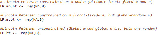
From these data we estimate a total population size using the Lincoln-Petersen estimator. Thus, the target for point and interval estimation is the true population size. As it happens, the same estimator is obtained whether you assume that: (1) Both m and n are fixed. (2) m is considered fixed, but n is not. And (3) Both m and n are considered random.

While the estimate of the total population for these three cases is identical, the uncertainty around it is not. Each set of assumptions fully determines the confidence intervals. We demonstrate this via parametric bootstrap (PB) because of how the levels of randomness enter at each stage is much more perspicuous in the PB code than in the corresponding analytic formulae.

Parametric Bootstrap

Compute the Lincoln-Petersen estimator for the sample at hand as well as the nuisance parameter phi.hat (the capture probability)

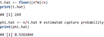
Now let’s set our PB simulation parameters to these two estimates:

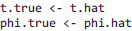
Next, set the total number of simulations

and then create empty arrays to store the three types of estimates

Finally, just turn the crank on the PB iterations and store them:

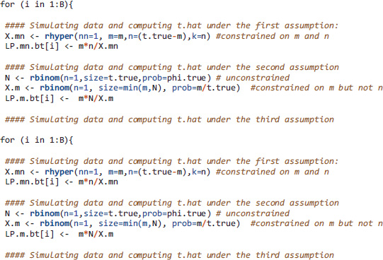
It is instructive to look at the sample spaces for these three estimators:

The sample spaces are all possible data sets that the simulations could generate under each of the model assumptions. The sample space for LP.m.bt is nested within that of LP.mn.bt, which is itself nested within the sample space of LP.bt. Clearly, global and local are relative terms. LP.m.bt is local with respect to LP.bt, but global with respect to LP.mn.bt.

The sampling distributions for the three estimators are plotted in the figure below. We now have three different confidence intervals. Which is right? Statistics by itself cannot answer that question. These three intervals represent the uncertainty in the hypothetical repetition of three different experiments. In the type 1 experiment, with m and n constrained, the only thing that can vary experiment to experiment is the number of marked animals in the final day sample.

In type 2, the number of previously marked individuals is constrained but not the final day sample size. The hypothetical experiment is repeated only for the final day; varying numbers of individuals as well as varying numbers of marked animals may be captured on the final day. In type 3, the entire hypothetical experiment is repeated. The number of marked individuals, the number of captured individuals, and the number of marked individuals in the second sample may all vary.

The appropriate interval depends on the kind of uncertainty you are trying to represent. The first interval answers the question: How different the estimators of the total population could be if someone else replicated the experiment such that the total number of marked individuals and total number of captures are identical to your experiment? This can happen in a field survey where the total number of marked animals and total number of captures is fixed by design, a priori. These numbers may depend on the budget the researcher might have for capturing animals for marking and for recapturing.

In some situations, such as camera trap surveys, the total number of marked animals may be fixed by design but the total number of captures, by the nature of the survey technique, is random. The second interval considers this possibility and allows for the randomness in the number of captures to compute the uncertainty in the total population size estimator. In the case of fish surveys, the number of fish caught in the traps or by electrofishing for marking is necessarily random and so is the number of fish in the sample afterwards. In this case, the third interval will be appropriate.

Figure Box 2.1

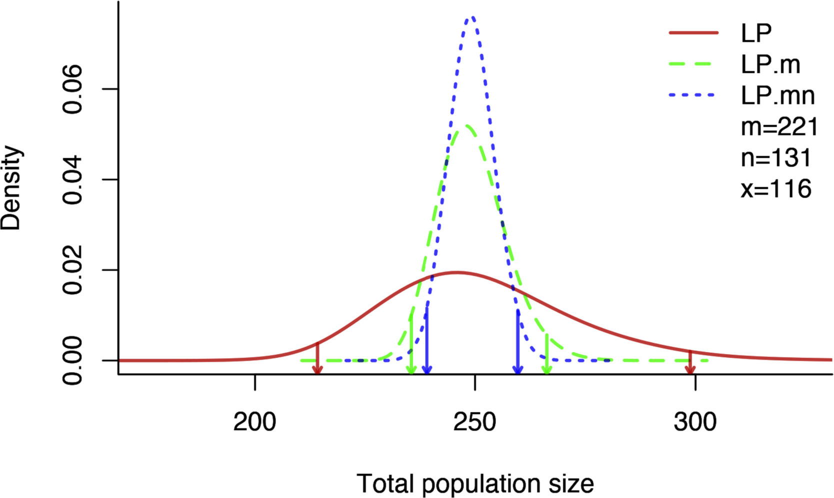
Figure Box 2.1 Sampling distributions and 95% confidence intervals of total population size estimates for three levels of conditioning in Lincoln Peterson estimates. The ML estimate for all three models is 249. The confidence 2.5 and 97.5% limits are indicated by the vertical lines dropped from each curve to the x-axis. The intervals become increasingly shorter as the models (hypothetical experiments) become more constrained. Here, as is generally but not universally the case, the intervals are completely nested.

2.2. Interpreting Evidential Uncertainty

Generally, desirable properties in confidence intervals are proper coverage and given proper coverage, shortness of length (Casella and Berger, 2002). A confidence interval can either cover the target or it can miss it. If the interval fails to cover the target, it can either be entirely above the target (miss high) or entirely below it (miss low) (see Figure 1). It is often, but not always, considered desirable if intervals that miss the target value are distributed equally above and below it. Evidence is one of the cases where an equal distribution of non-coverage is undesirable. In this context missing high is superior to missing low. Both types of intervals misrepresent the confidence one should have in the evidence, but the high miss is at least always indicating a correct assessment while a low miss could be supporting an incorrect assessment. Of course, this is assuming the expected evidence is positive, as in Figure 1, if the expected evidence were negative, the desirability of missing high and low would be reversed. Really, we mean that it is better for the interval to miss its target distally from 0 than to miss proximally to 0. However, in this simulation study the evidential comparisons are arranged so the reference model is always the better model as to keep the language of missing high and low less confusing.

FIGURE 1

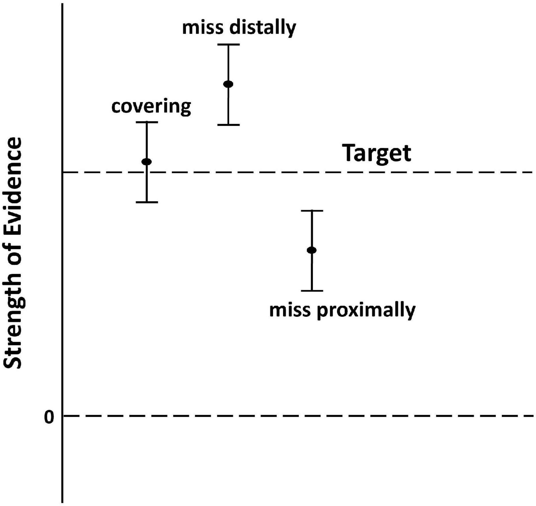
Figure 1. Hypothetical coverage of confidence intervals for evidence. The strength of evidence is the value of an evidence function relating two models and a data set. Typical evidence functions are LLR or the difference of information criterion values, ΔICs. In our worked example (Section 3) we use the Schwarz information criterion. ΔSIC_RA values greater than 0 indicate support in the data for the reference model relative to the alternative. These values are indicated by dots in the figure. The vertical bars indicate confidence intervals for the strength of evidence. The target for a confidence interval on the strength of evidence is a penalized scaled divergence difference (see Section 4.1), loosely this is the expected evidence. By design, a perfect confidence interval, at say the 95% confidence level, will fail to cover its target 5% of the time. If a confidence interval that misses its target is entirely more distant from 0 than is its target, we say that it misses distally, otherwise we say that it misses proximally. We will also speak of the bound of a confidence interval for evidence that is closest to 0 as the proximal bound.

The categories of evidence introduced in Box 1 suggest useful ways to apply confidence intervals for strength of evidence to scientific inference. Scientifically, the paramount question is: is the evidence veridical (i.e., in agreement with fact) or is it misleading? The intervals we propose estimating can give us confidence in our answer. We propose that if the proximal bound of this confidence interval is distal to k_S that it be considered “very secure.” If the proximal bound falls between k_S and k_p then the evidence should be considered “secure.” Finally, if the proximal bound is proximal to k_p or the interval overlaps 0 the evidence is “insecure.”

These three levels of strength of evidence and two levels of security of evidence create six heuristic categories:

1. Strong and very secure (SV): The point estimate of evidence (e.g., ΔSIC) is strong and the lower bound of uncertainty indicates that we have confidence that the target (true evidence) is also strong.

2. Strong and secure (SS): The point estimate of evidence is strong, and we are confident that the true target is at least prognostic. There is very little chance that this evidence is misleading.

3. Strong but insecure (SI): The point estimate of evidence is strong, but we cannot be confident that the target is not weak.

4. Prognostic and secure (PS): The point estimate of evidence is prognostic, and we can be confident that the target is at least prognostic.

5. Prognostic but insecure (PI): The point estimate of evidence is prognostic, but we are not confident that the target is not weak.

6. Weak and insecure (WI): The point estimate of evidence is weak and thus by definition, we are not confident that the target is not weak.

As sample size increases, a majority of the sampling distribution lies above the strong evidence threshold and the probability of obtaining evidence that is not SS diminishes to 0 (Dennis et al., 2019). There is, of course, the pathological case where two models are equally divergent from the true generating process. Were this curiosity ever to occur, then each model would be strongly and securely selected with probability 0.5. It is arguable that, even in such a situation, no error has occurred, as in each case a model closest to the generating process has been selected. Substantial discussion on interpreting statistical evidence when augmented with confidence intervals is given in Box 3.

BOX 3. Interpreting evidence using confidence intervals.

Figure Box 3.1

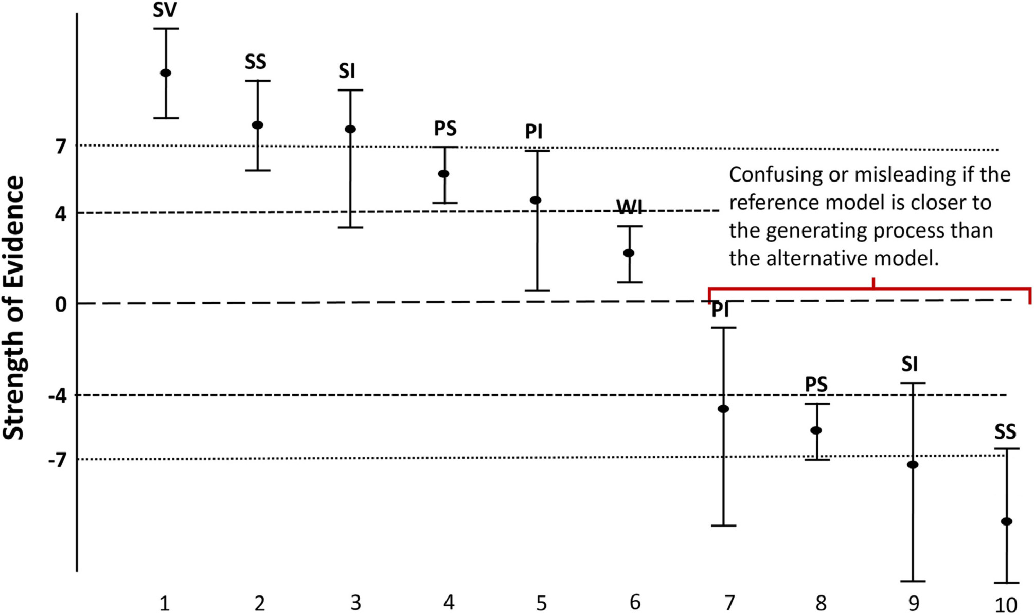
Figure Box 3.1 depicts some hypothetical confidence intervals for the strength of evidence. The boundaries for the evidential categories are set as: strong evidence for the alternative = −k_S = –7, prognostic evidence for the alternative = −k_p = –4, prognostic evidence for the reference = k_p = 4, and strong evidence for the reference = k_p = 7.

In interval 1, the observed evidence (e.g., ΔSIC), indicated by the filled oval, is strong and the lower bound for the confidence interval is above the strong evidence threshold. This evidence is designated strong and very secure (SV)—the reference model is strongly supported as being closer to the generating process than the alternative and there is almost no chance that sampling variation would upset this identification. In this case, the researcher may reasonably conclude that no further work is needed regarding model identification in this particular model contrast. Possibly, further work may be indicated to improve parameter estimate precision in the identified better model.

In interval 2, the observed evidence is above the strong evidence threshold, and the proximal bound is greater than the prognostic evidence threshold. We call this situation “strong but secure” (SS). This implies that the reference model is strongly supported, and it is unlikely (but plausible) that this is due to sampling variation. Cautious but optimistic interpretation is indicated, and if possible, more data should be collected to confirm the conclusions.

In interval 3, the observed evidence is above the strong evidence threshold, but the proximal bound is less than the prognostic evidence threshold. We call this situation “strong but insecure” (SI). This implies that while the reference model is strongly supported, it is uncertain due to sampling variation. Very cautious interpretation is indicated, and if possible, more data should be collected to confirm the conclusions.

In interval 4, the observed evidence is less than the strong evidence threshold, and the proximal bound is greater than the prognostic evidence threshold. We call this situation “prognostic but secure” (PS). This implies that while the reference model has only moderate support, it is unlikely that this is due to sampling variation. In this case, the distal bound is less than the strong evidence threshold. It is likely that both models explain the data nearly equally well, but with a slight edge to the favored model.

In interval 5, the observed evidence is less than the strong evidence threshold, and the proximal bound is less than the prognostic evidence threshold. We call this situation “prognostic but insecure” (PI). This implies that the reference model has only moderate support and even this may be due to sampling variation. The primary implication is that more data is needed either within the context of the current experiment or by combining these results with the results of other experiments.

In interval 6 the evidence is weak and insecure (WI). The models are not differentiated by the data. The researcher should collect more data in order to identify the models. The researcher should of course recognize that not all data is equally informative and seek data that will distinguish the two models (e.g., Cooper et al., 2008). Another choice that could be made, particularly if large amounts of data have already been collected, is to decide that both models are adequate for the intended purposes (Lindsay, 2004; Markatou and Sofikitou, 2019).

Intervals 7, 8, 9, and 10 are reflections of intervals 5, 4, 3, and 2, only in this case they are misleading. The designation C stands for confusing evidence, which is prognostic evidence for the wrong model. The designation M stands for misleading evidence, which is strong evidence for the wrong model.

Interval 10 is a researcher’s worst case. The evidence is strong, secure and misleading. The researcher should try to avoid this situation both by experimental design (large sample size, treatments or observations that strongly differentiate between the models) and by analytic design (higher strong and marginal evidence thresholds).

In practice, we do not know if the evidence is misleading or not. For this discussion, we consider “negative” evidence as misleading but in fact, it only indicates that it supports the alternative model—unless one knows the location of the generating process (see Ponciano and Taper, 2019). Simulations (Section 5.2 and Taper et al., 2019) show that for global evidence strong but secure misleading evidence occurs very rarely—regardless of whether the model set is correctly specified or misspecified. For local evidence if the model set is correctly specified, secure misleading evidence is exceedingly rare. However, under model misspecification secure misleading evidence occurs more frequently, although it is still not common. We present an explicit comparison of global and local inference under correctly specified and misspecified models in Section 5.2.

3. Example: Uncertainty in a Structural Equations Models Analysis of Post-Fire Recovery of Plant Diversity

To probe the effectiveness of bootstrapping evidence in realistically complex problems, we revisit the classic analysis of Grace and Keeley (2006). These authors used structural equation modeling to study the impact of landscape, environment, and community factors on the recovery after fire of shrubland plant diversity.

A recent article on developing causal models (Grace and Irvine, 2020) revisits the 2006 study and takes a more moderate stance than the original paper: “Subsequent SEM studies (Keeley et al., 2008) have enhanced our confidence in the general inferences drawn from the original study. That said, we would not claim that all our parameter values are unbiased causal estimates without further evidence to support such inferences.” We believe that had Grace and Keeley had the tools for estimating the two kinds of evidential uncertainties we have developed here a much more nuanced understanding could have been gained—even from the original data—as to which paths were likely to be supported by future work and which were potentially non-replicable.

3.1 Example Choice

There are reasons why SEM is growing in influence in environmental informatics, ecology and evolution. First, SEM allows for legitimate causal inference in situations both in observational studies (Grace, 2008; Bollen and Pearl, 2013; Grace and Irvine, 2020) and where experimental manipulation has been performed (Grace et al., 2009; Breitsohl, 2019). In fact, path analysis, the precursor to SEM, was first developed by Sewall Wright (1934) to expose causal effects to statistical inference. Second, because it is designed for estimation of a network of causal effects, SEM is well suited for analyses of the complex patterns of influence often found in environmental science, ecology and evolution (e.g., Grace and Pugesek, 1997). Third, SEM recognizes that many observables may be recorded with measurement error (Bollen, 1989). The ability to incorporate measurement error in an analysis eliminates an important source of bias that has plagued environmental science, ecology and evolution (Taper and Marquet, 1996; Cheng and Van Ness, 1999). Implicit in the incorporation of measurement error is the ability to consider latent variables (i.e., unobserved, and potentially unobservable variables) (Grace and Bollen, 2008; Grace et al., 2010). Fourth, causal paths and latent variables allow linking scientific theory and statistical analysis in a particularly perspicuous fashion (Grace and Bollen, 2008; Grace et al., 2010; Laughlin and Grace, 2019). Because of these beneficial features, SEM is being utilized in growing number of applications in environmental informatics, ecology and evolution. The explosive growth of SEM in ecology is documented in Laughlin and Grace (2019).

Despite its many advantages for scientific thinking, SEM does present some inferential difficulties (Tomarken and Waller, 2003). Information can flow between variables by multiple pathways. As a consequence, the fit of alternative models and therefore the evidence between them can vary considerably with small changes in the configurations of the data. This uncertainty in evidence needs to be quantified.

A final reason for the choice of the Grace and Keeley example is the excellence of the original study. The observations were collected under the direction of Jon Keeley, while the analysis was conducted by James Grace. Jon Keeley is a very experienced empirical ecologist, while Grace has been a leading proponent the application of SEM to ecological systems. Both are scientists of great distinction. We do not seek to cavil at pedestrian research but look to see what bootstrapping of evidence can add to a well done scientific analysis.

3.2. Example Description

Keeley et al. (2005) and Grace and Keeley (2006) describe the data collection in detail. In brief, 90 sites in southern California were surveyed for 5 years following wildfire. Seven variables were observed indicating 7 latent variables (see Table 1). Variables were transformed to generate approximate linear homoscedastic relationships.

TABLE 1

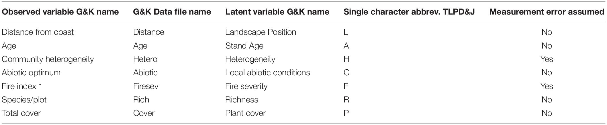
Table 1. Descriptions of variables from Grace and Keeley (2006).

3.3. Model Naming Conventions

We will use a model naming convention that indicates latent variable regression structure. The single character abbreviation for a variable will be followed by “.” and then by the abbreviations for the variables it is regressed on. Regressions with different response variables will be separated by “_.”

If a latent is isolated, that is it is neither a response nor a predictor in any regression in the model, its character would be entered in the model name but not followed by a “.” We don’t consider any such models, because we are picking up the Grace and Keeley reanalysis mid-stream, after they eliminated a variable called “Community Type” from their analysis. Alphabetical order will be imposed so that a path model uniquely determines a name. Thus the Grace and Keeley best model can be named: “A.L_C.L_F.A_H.L_P.F_R.CHLP” (see Figure 2 and Table 1).

FIGURE 2

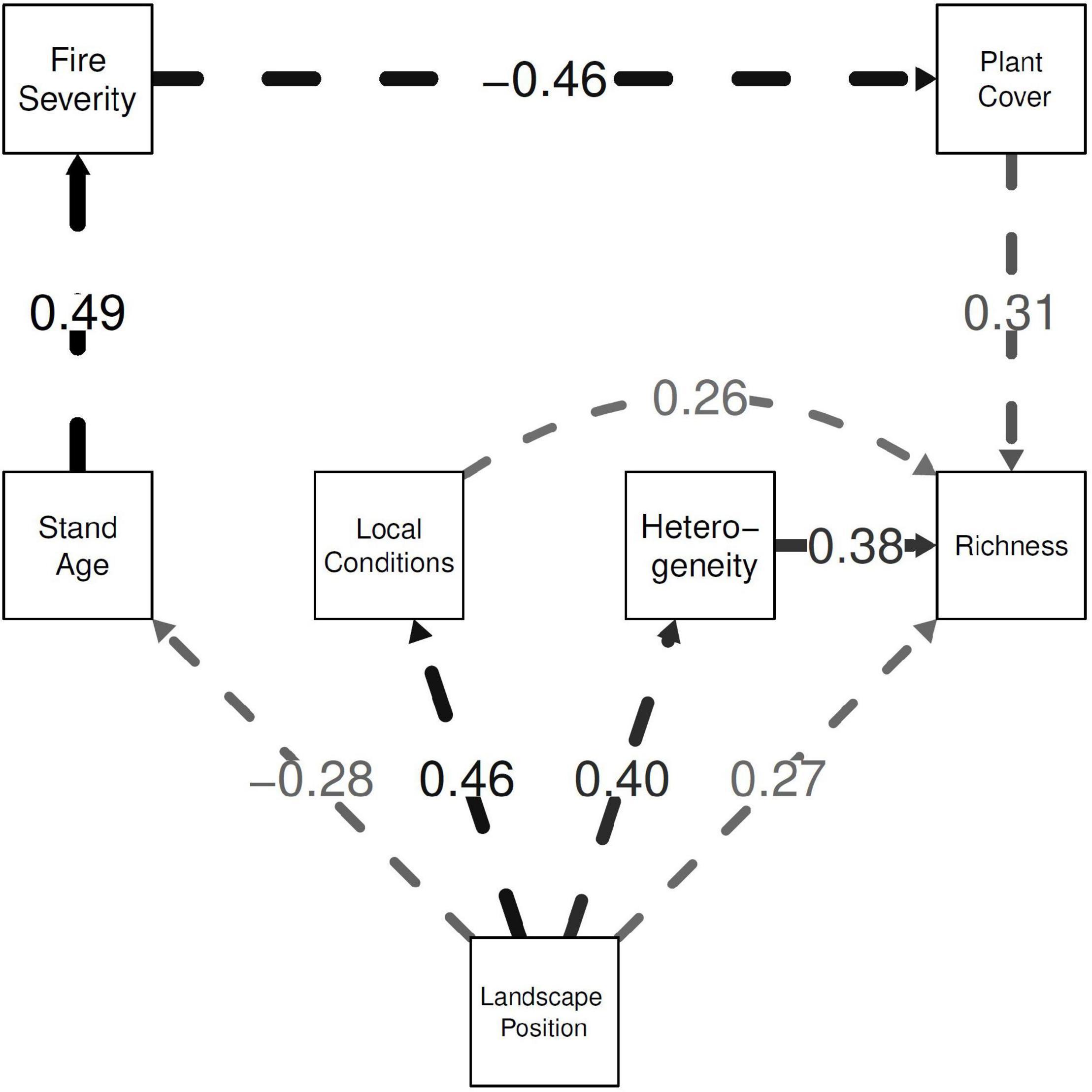
Figure 2. The estimated final, simplified model explaining plant diversity. Arrows indicate causal influences. The standardized coefficients are indicated by path labels and widths. Weak paths with coefficients of magnitude less than 0.30 are shown in gray.

3.4. Example Reanalysis

Dr. Grace kindly provided the original data set and his original code (written using R package lavaan). In our reanalysis we use the R package lava (version 1.6.7). The estimates of the standardized coefficients from the two packages agree to at least the 5 decimal places reported by lava. Grace and Keeley determine their best model based on several factors including theoretical background, chi-square model adequacy tests, generalized likelihood ratio tests between nested models, and inspection of deviations between observed and model implied covariances. Grace and Keeley note the consistency of their model identification with identification based on information criterion.

The strong theoretical relationship between ΔICs, the difference of information criterion values, and the likelihood ratio test statistic has been noted before (e.g., Burnham and Anderson, 2002; Lele and Taper, 2012; Taper and Ponciano, 2016). What differs between the approaches are the assumptions and warrants that tie the statistics to scientific inference. These differences can lead to substantive differences in inference from the same data and essentially the same statistic. With a NP test you inference is a categorical accept or reject if your p-value is 0.051, just the wrong side of alpha of 0.05 your reject. If you have a ΔIC of 6.9, you don’t reject it instead you give a more elaborate discussion: “Well the evidence doesn’t quite reach our arbitrary strong evidence threshold, but it is very strong prognostic evidence.” We will return to this in the discussion (see also Box 1). Here we focus on the impact of uncertainty in evidence for one model over another given the data on reasonable scientific inference.

3.4.1. Models Considered

Statistical evidence, at least defining the term as in the Royall (1997), Lele (2004a), Taper and Ponciano (2016), and Brittan and Bandyopadhyay (2019) tradition, is not unary, but binary: It measures the support (Edwards, 1992) for one model over another model that is given by data. The models we compare are listed in Table 2.

TABLE 2

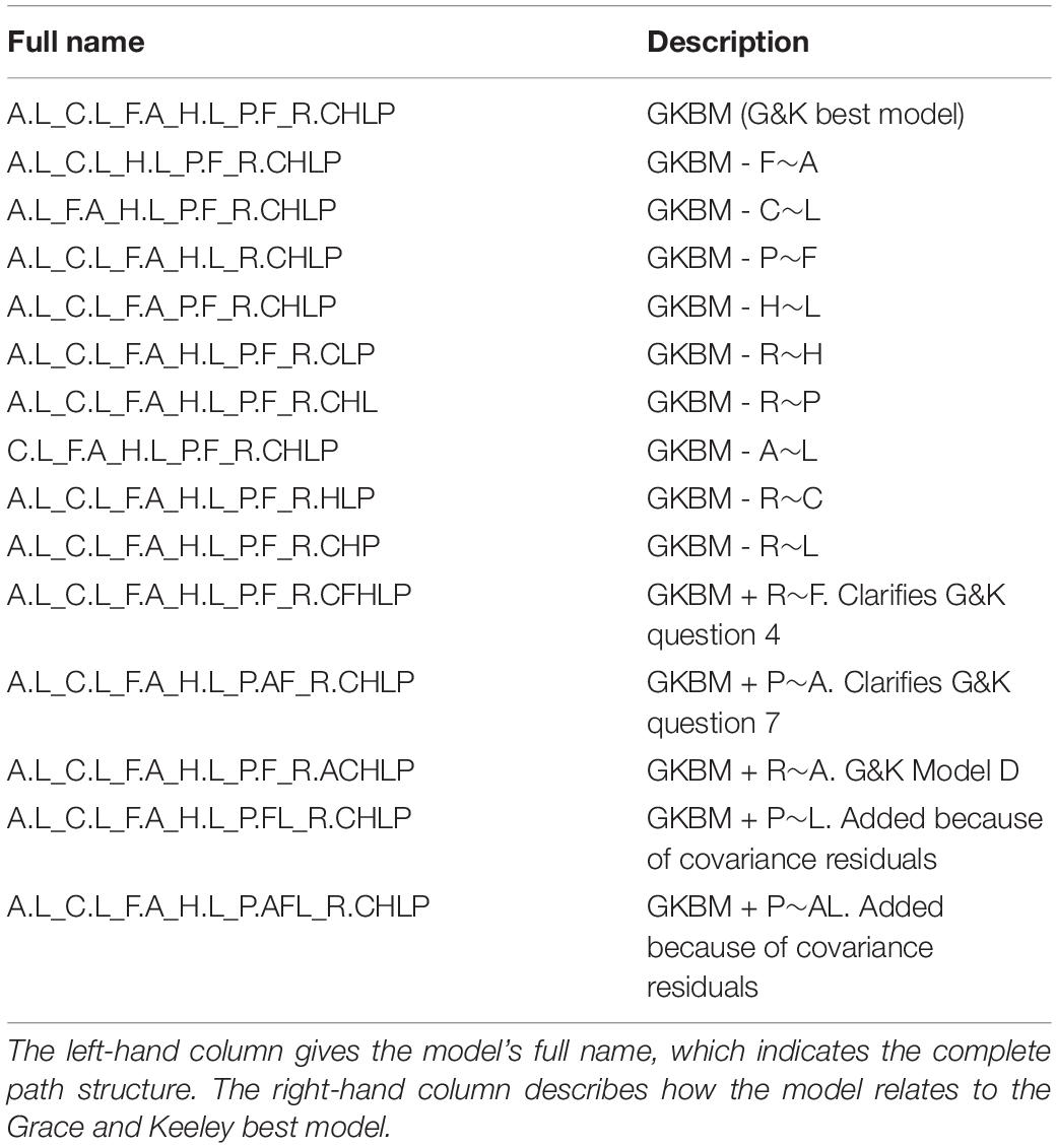
Table 2. Models compared in our reanalysis of the Grace and Keeley (2006) structural equation analysis of diversity recovery after fire.

The first model is the Grace and Keeley best model (GKBM). The next 9 models are deletion models that each differ from the best model by the absence of a single path. These models are listed in order (strongest to weakest) of the strength of the effect in the best model (as measured by the coefficient z-statistic). Comparison of each of these models with the GKBM will probe the question of whether the deleted path belongs in “best model.” The last 5 models are addition models that each differ from the GKBM by the presence of 1 or 2 paths. Comparison of each of the addition models with the GKBM probes the question of whether that/those paths should be included in a “best model.”

3.4.2. Example Reanalysis Results

The results of our reanalysis are presented in Figure 3, which plots the evidence (ΔSIC) and its uncertainty for the GKBM relative to each of the deletion models, and Figure 4, which shows GKBM evidence and uncertainty relative to the addition models.

FIGURE 3

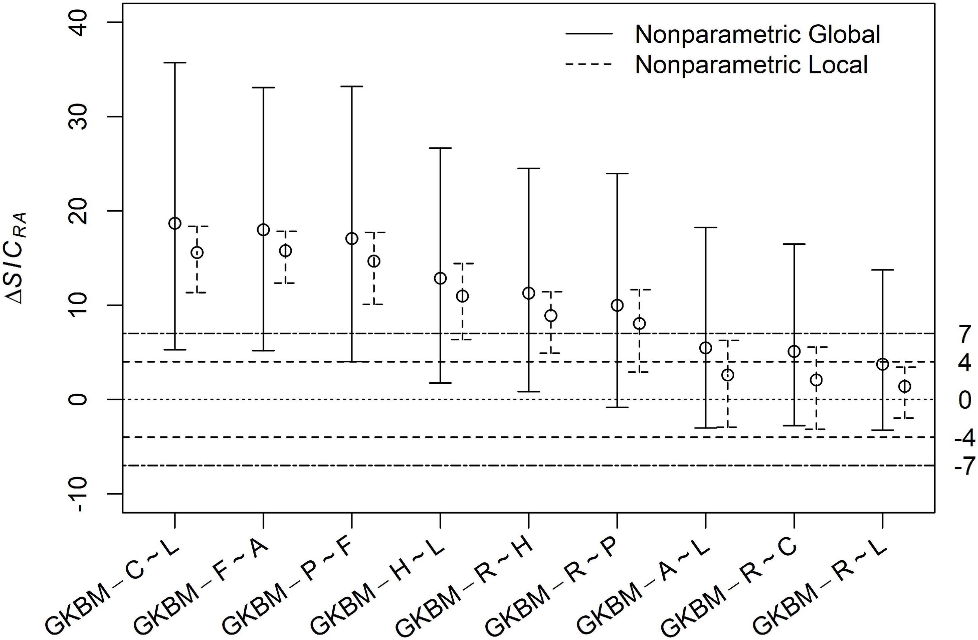
Figure 3. Evidential uncertainty intervals comparing the Grace and Keeley best model with 9 models, each that deletes one of the paths in the GKBM. For each model comparison, the open circle indicates the observed evidence, the solid error bar indicates the global uncertainty, the dashed error bars show the local uncertainty. These are approximate 90% confidence intervals based on 4000 non-parametric bootstraps. The strong evidence thresholds are indicated by dot-dash horizontal limit lines at 7 and -7, while the prognostic evidence thresholds are indicated at dashed limit lines at 4 and -4. Positive values of the ΔSIC_RA indicate evidence for the GKBM, as the reference model, relative to the alternative model, while negative values indicate evidence for the alternative model relative to the GKBM. The separatrix between these two regions is the dotted horizontal limit at 0.

FIGURE 4

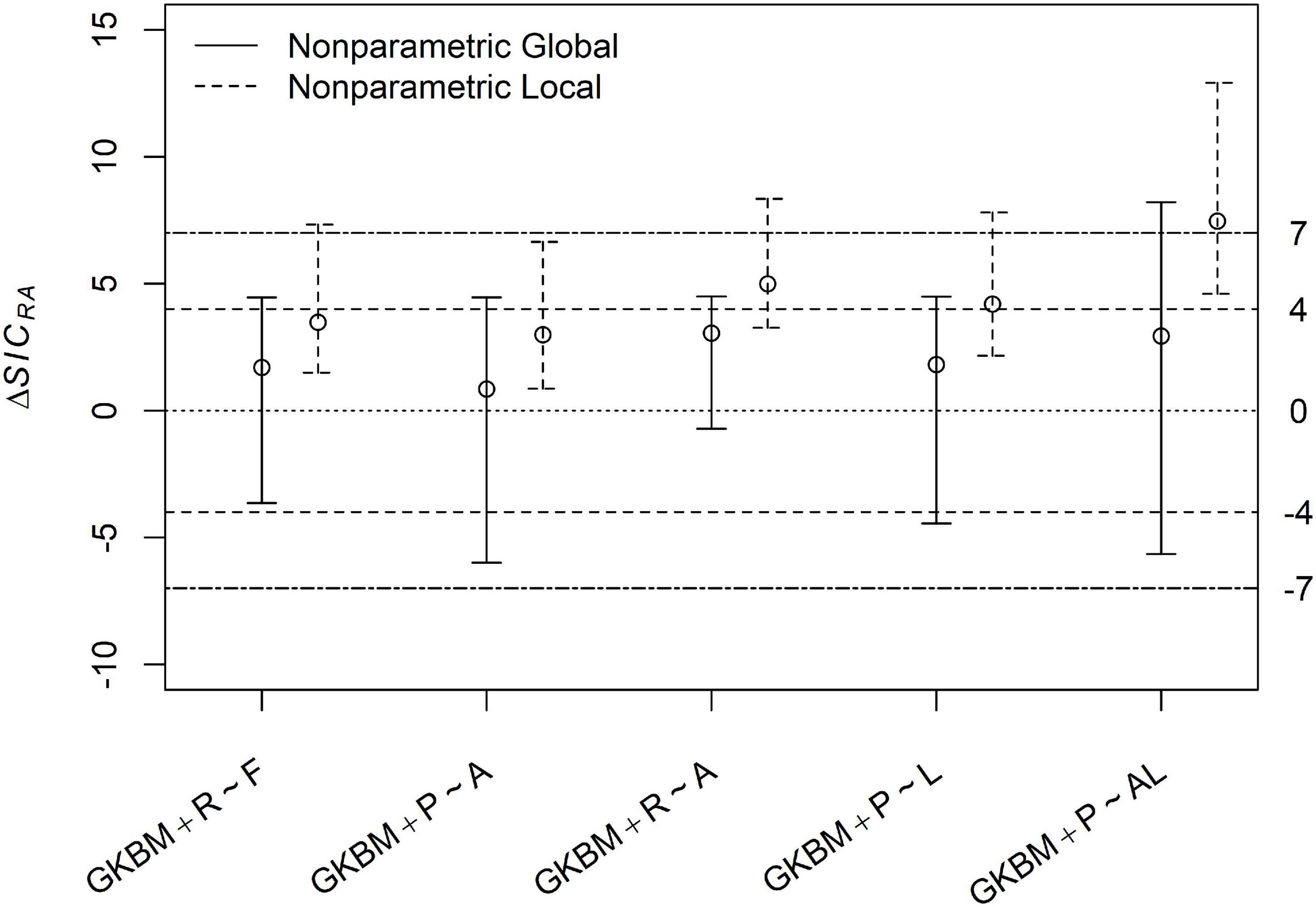
Figure 4. Evidential uncertainty intervals comparing the Grace and Keeley best model with 5 models, each that adds one or two paths to the GKBM.

The first three model comparisons are rock solid. They all have strong and secure global evidence and strong and very secure local evidence. Not only does this data set strongly favor including these three paths, but replication of the experiment—in the same environment—will almost always reach the same conclusion.

The next two comparisons (GKBM - H∼L and GKBM - R∼H) both have strong and secure local evidence for including their paths, but globally, they are insecure. We have good reason to believe that these paths represent real causal effects, but need to advise researchers seeking to replicate this experiment to increase sample size to avoid equivocal results.

Then a comparison (GKBM - R∼P) with evidence, both global and local, that is strong but insecure. Here the global interval crosses the 0 line. Researchers should consider the possibility that the path may be weaker than estimated or may be non-existent.

The next two comparisons have barely prognostic evidence for their paths, but are insecure both globally and locally, with intervals that substantially overlap the line separating evidence for one model versus evidence for the other. The final comparison has positive but weak evidence for inclusion of the path. It is by definition insecure. The local evidence interval falls entirely between the two prognostic evidence thresholds. There is evidence for the path, but it is just a bit more than a toss-up.

Whether or not the last 3 paths should be included in a model is a judgment call for the reporting researchers based on the costs both practical and intellectual of including false paths or omitting true paths. For these deletion paths, a nudge might be given toward including them because the evidence favors the more complex model despite the SIC evidence function being used having a slight bias at small sample size toward compact models.

All five addition models have global evidence that is weak and insecure but that leans toward the more compact GKBM. However, all the global intervals overlap the separatrix at 0, and three of the intervals even overlap the marginal evidence thresholds for including the paths. The local evidence shifts slightly further toward the GKBM.

At this sample size, there is no compelling statistical reason to include any of the addition paths in the “best model,” but there is also no compelling statistical reason not to. The slight tilt toward the GKBM may represent nothing more that the SIC bias toward compact models. It is very hard statistically to distinguish between the true absence of a path and the presence of a weak path. It would take a sample size of more than 1,000 for there to be an expectation of global strong and secure SIC evidence for the absence of a path even if it was truly absent. On the other hand, because the coefficient of variation of local evidence declines at a much faster rate than that of global evidence (n^–1 versus n^–1/2) even a modest increase in sample size may allow local identification of weak effects. In the case of the Grace and Keeley example the breadth of the conditional intervals indicates that the sample size is marginal in a statistical sense—despite the Herculean effort represented.

Models are single entities, but they are entities built from components. In our experience, a great deal of insight into how components function in models can be found by estimating the evidence for a model including the component relative to the same model without that component. In all 14 model comparisons, the weight of evidence tilts toward the GKBM. We agree with Grace and Keeley that A.L_C.L_F.A_H.L_P.F_R.CHLP is the “best model” (at least out of those considered) to describe the structural relationships in this data set. Grace and Keeley chose in 2006 to interpret the empirical results of their study narrowly. “Ultimately, results and interpretations presented in this paper are based on the model judged to be the best representation of the data” (Grace and Keeley, 2006). Here we do disagree with Grace and Keeley. Our analysis has shown that even within a small list of a priori models, drawn from their own back-ground theory, there are multiple plausible models whose interpretation should be considered. To interpret only a single best model is like choosing to use only a parameter point estimate without considering its uncertainty. It is simple, but over-confidence can be generated.

4. Mathematical Development

In this section, we develop the statistical justification and estimation algorithms for the confidence intervals for evidence that we use in this paper. A reader satisfied with a simulation-based justification could skip to Section 5, at least on first reading.

Different statistical divergences could be used to construct model adequacy measures and thus evidence functions (see Lele, 2004a; Markatou and Sofikitou, 2019). Each will have its own properties, and each could be useful in different circumstances. In this paper we focus on the Kullback-Leibler divergence (KLD) as it leads to the information criteria, evidence functions already in common use. The treatment of uncertainty for other divergences and evidence functions should parallel that for the KLD. The mathematical notation, definitions, and assumptions used in our treatment are given in Box 4.

BOX 4. Mathematical notations, definitions, and assumptions.

The notation in this box is more verbose than commonly used to allow the reader to track fine distinctions among generating process, distribution estimators, estimated distributions for a particular sample, true parameters, parameter estimators and parameter estimates given a particular sample.

(1) Data are assumed to be suitable for non-parametric bootstrapping. For this paper we further assume that the data are independently and identically distributed (i.i.d.).

(2) Probability density function (pdf) or probability mass function (pmf) representing the true generating mechanism is denoted g(.). Its cumulative distribution function (cdf) is denoted as F_g(⋅).

(3) Observed data: $\underset{¯}{x}=(x_1,x_{2,}\mathrm{\dots },x_n)$, where n denotes the sample size.

(4) Random variables: $\underset{¯}{X}=(X_1,X_{2,}\mathrm{\dots },X_n)$.

(5) The pdfs/pmfs for reference (R) and alternative (A) models are denoted by m_R(.) and m_A(.), respectively. For example, m_R is N(μ = 5, σ = 1). Note, these are fully specified models.

(6) If the reference and alternative model are not fully specified, then they represent model spaces denoted M_R and M_A respectively. In that case each of M_R and M_A is a collection of models. For example, M_R = N(μ, σ)) with μ in (−∞, ∞) and σ in (0, ∞).

(7) $F_g^{\left(n\right)}(t;\underset{¯}{X})=\frac{1}{n}{\sum }_{i=1}^{n}I(X_i\le t)$ is the empirical estimator of the cdf of g(.) for a random vector of length n. Here I(A) is the indicator function for event A. Denote a corresponding numerically smoothed density as $g_{n,\underset{¯}{X}}(.)$.

(8) ${\widehat{F}}_g^{\left(n\right)}(t;\underset{¯}{x})=\frac{1}{n}{\sum }_{i=1}^{n}I(x_i\le t)$, the empirical estimate of the cdf of g(.) for an observed vector of length n. Denote a corresponding numerically smoothed density as ${\widehat{g}}_{n,\underset{¯}{x}}(.)$.

(9) The KLD between two specified continuous models, where the reference model is m_R is K(m_R, m_A) = ∫(log⁡(m_R(x)) − log⁡(m_A(x)))m_R(x)dx. In general, for any two models (discrete, continuous or piecewise continuous) we write K(m₁, m₂) = ∫(log⁡(m₁(x)) − log⁡(m₂(x)))dF_m1(x).

(10) The KLD orthogonal projection of a probability distribution, such as a fully specified model, s(.) onto a model space M is $m_s^{*}=\underset{m\in M}{\arg \min }K(s(.),m)$ (see Figure 3 in Ponciano and Taper, 2019). This model is the closest approximation to s(.) in the model space M.

(11) If $s(.)\in M\Rightarrow m_s^{*}(.)\equiv s(.)$. If the generating process is in either M_R or M_A that is if either g(.) ∈ M_R or g(.) ∈ M_A then the model set {M_R, M_A} is considered correctly specified, as in the foundations of much classical statistics (e.g., Neyman and Pearson, 1933; Wilks, 1938; Wald, 1943).

(12) The log-likelihood function for the observed data, $\underset{¯}{x}$, under g(.) is $l_g\left(\underset{¯}{x}\right)={\sum }_{i=1}^n\log \left(g\left(x_i\right)\right)$

The log-likelihood function for the observed data under a model m(.) is $l_m\left(\underset{¯}{x}\right)={\sum }_{i=1}^n\log \left(m\left(x_i\right)\right)$. ${\widehat{m}}_{\underset{¯}{x}}(.)$ is the model with parameter values that maximizes $l_m\left(\underset{¯}{x}\right)$.

(13) Conceptually, ${\widehat{m}}_{\underset{¯}{x}}(.)$ is the same model as $m_{{\widehat{g}}_{n,\underset{¯}{x}}}^{*}$. The first notation is more familiar, the second emphasizes that the maximum likelihood model is a projection of the model to the empirical density. Asymptotically these estimates will be identical, but there will be slight numerical differences at finite sample size due to the smoothing in ${\widehat{g}}_{n,\underset{¯}{x}}$.

(14) The KLD estimator of the divergence of a model, m, from the generating process, g is given as

$\begin{array}{ccc}\hfill K({\widehat{g}}_{n,\underset{¯}{X}},m;\underset{¯}{X})& \hfill =\hfill & \int \log \left({\widehat{g}}_{n,\underset{¯}{X}}(t)\right)d{F}_g^{\left(n\right)}(t;\underset{¯}{X})-\int \log \left(m(t)\right)d{F}_g^{\left(n\right)}(t;\underset{¯}{X})=S_{{\widehat{g}}_{n,\underset{¯}{X}}}{,}_{{\widehat{g}}_{n,\underset{¯}{X}}}-S_{{\widehat{g}}_{n,\underset{¯}{X}}}{,}_m\hfill \end{array}$

where S_ĝn,X,ĝn,X is the neg-self-entropy of the generating process and S_gn,X,m is the neg-cross-entropy from the generating process to the model m. Note, an estimator is the function of a random variable (i.e., $\underset{¯}{X}$) that returns an estimate for a particular realization of the random variable.

(15) The KLD estimate of the divergence of a model, m, from the generating process, g:

$\begin{array}{ccc}\hfill K({\widehat{g}}_{n,\underset{¯}{x}},m;\underset{¯}{x})& \hfill =\hfill & \int \log \left({\widehat{g}}_{n,\underset{¯}{x}}(t)\right)d{\widehat{F}}_g^{\left(n\right)}(t;\underset{¯}{x})-\int \log \left(m(t)\right)d{\widehat{F}}_g^{\left(n\right)}(t;\underset{¯}{x})=S_{{\widehat{g}}_{n,\underset{¯}{x}}}{,}_{{\widehat{g}}_{n,\underset{¯}{x}}}-S_{{\widehat{g}}_{n,\underset{¯}{x}}}{,}_m\hfill \end{array}$.

where $S_{{\widehat{g}}_{n,\underset{¯}{x}}{\widehat{g}}_{n,\underset{¯}{x}}}$ is the neg-self-entropy of the empirical distribution.

(16) The KLD projection estimator of the divergence of a model space, M, from the generating process, g: $K({\widehat{g}}_{n,\underset{¯}{X}},M;\underset{¯}{X})=S_{{\widehat{g}}_{n,\underset{¯}{X}},{\widehat{g}}_{n,\underset{¯}{X}}}-S_{{\widehat{g}}_{n,\underset{¯}{X}},m_{{\widehat{g}}_{n,\underset{¯}{X}}}^{*}}$

(17) The KLD projection estimate of the divergence of a model space, M, from the generating process, g: $K({\widehat{g}}_{n,\underset{¯}{x}},M;\underset{¯}{x})=S_{{\widehat{g}}_{n,\underset{¯}{x}},{\widehat{g}}_{n,\underset{¯}{x}}}-S_{{\widehat{g}}_{n,\underset{¯}{x}},m_{{\widehat{g}}_{n,\underset{¯}{x}}}^{*}}$

(18) One estimate for $K({\widehat{g}}_{n,\underset{¯}{x}},M;\underset{¯}{x})$ is $S_{{\widehat{g}}_{n,\underset{¯}{x}}{\widehat{g}}_{n,\underset{¯}{x}}}-l_{\widehat{m}\left(\underset{¯}{x}\right)}$, see discussion in definition (13). Bias correction for this estimate is the goal of information criteria. We employ the consistent family of bias correction terms c_np, where c_n is a function of n growing strictly between loglog(n) and n. And, p is the parametric dimension of M (Nishii, 1988).

(19) The global penalized scaled divergence difference target: ΔD_Pn(g, M_R,M_A, n) = 2n{K(g, M_A)−K(g, M_R)} + c_n(p_A−p_R) (see definition 16). The target is the quantity for which we attempt to find both a central estimate and an uncertainty measure (see discussion in Section 4.1). Note that for fully specified model comparisons, the penalty term is 0, and ΔD_Pn(g, m_R, m_A, n) = 2n{K(g, m_A)−K(g, m_R)}

(20) The local penalized scaled divergence difference target, $\mathrm{\Delta }{d}_{Pn}(g,M_{R,}{M}_A,\underset{¯}{x})=2n\{K(g,M_A,\underset{¯}{x})-K(g,M_R,\underset{¯}{x})\}+c_n(p_A-p_R)$ (see definition 17).

(21) The global penalized divergence difference estimator, $\mathrm{\Delta }{D}_{Pn}({\widehat{g}}_{n,\underset{¯}{X}},M_{R,}{M}_A,\underset{¯}{X})=E_{{\widehat{g}}_{n,\underset{¯}{X}}}\left(2n\{K({\widehat{g}}_{n,\underset{¯}{Y}},M_A,\underset{¯}{Y})-K({\widehat{g}}_{n,\underset{¯}{Y}},M_R,\underset{¯}{Y})\}+c_n(p_A-p_R)\right)$. Note that inside the expectation $\underset{¯}{Y}$ is a random vector drawn from ${\widehat{g}}_{n,\underset{¯}{X}}$.

(22) The local penalized divergence difference estimator, $\mathrm{\Delta }{d}_{Pn}({\widehat{g}}_{n,\underset{¯}{X}},M_{R,}{M}_A,\underset{¯}{x})=E_{{\widehat{g}}_{n,\underset{¯}{X}}}\left(2n\{K({\widehat{g}}_{n,\underset{¯}{Y}},M_A,\underset{¯}{x})-K({\widehat{g}}_{n,\underset{¯}{Y}},M_R,\underset{¯}{x})\}+c_n(p_A-p_R)\right)$. Note that inside the expectation $\underset{¯}{Y}$ is a random vector drawn from ${\widehat{g}}_{n,\underset{¯}{X}}$.

(23) The global evidence estimate, $\begin{array}{ccc}\hfill E{v}_G(M_R,M_A;{\widehat{g}}_{n,\underset{¯}{x}},\underset{¯}{x})& \hfill =\hfill & E_{{\widehat{g}}_{n,\underset{¯}{x}}}\left(2n\{K({\widehat{g}}_{n,\underset{¯}{Y}},M_A,\underset{¯}{Y})-K({\widehat{g}}_{n,\underset{¯}{Y}},M_R,\underset{¯}{Y})\}+c_n(p_A-p_R)\right)\hfill \\ & & =E_{{\widehat{g}}_{n,\underset{¯}{x}}}\left(-2\{l_{{\widehat{m}}_{A_{\underset{¯}{Y}}}}\left(\underset{¯}{Y}\right)-l_{{\widehat{m}}_{R_{\underset{¯}{Y}}}}\left(\underset{¯}{Y}\right)\}+c_n(p_A-p_R)\right)\hfill \end{array}$. Note that inside the expectation $\underset{¯}{Y}$ is a random vector drawn from ${\widehat{g}}_{n,\underset{¯}{x}}$ and that the maximum likelihood estimate, ${\widehat{m}}_{\underset{¯}{x}}$, has been substituted for $m_{{\widehat{g}}_{n,\underset{¯}{x}}}^{*}$ (see definitions 13 and 18). Both the estimated models and the data from which the likelihoods are calculated are random. Thus, variation in Ev_G is due to both variation in $\underset{¯}{Y}$ and to variation in the estimates of ${\widehat{m}}_{A_{\underset{¯}{Y}}}\text{and}{\widehat{m}}_{R_{\underset{¯}{Y}}}$. Non-parametric bootstrap will be used to estimate the expectation and its uncertainty estimation and for further bias reduction. Positive values for evidence indicate that the reference model is supported over the alternative model (see discussion Box 1).

(24) The local evidence estimate, $\begin{array}{ccc}\hfill E{v}_L(M_R,M_A;{\widehat{g}}_{n,\underset{¯}{x}},\underset{¯}{x})& \hfill =\hfill & E_{{\widehat{g}}_{n,\underset{¯}{x}}}\left(2n\{K({\widehat{g}}_{n,\underset{¯}{Y}},M_A,\underset{¯}{x})-K({\widehat{g}}_{n,\underset{¯}{Y}},M_R,\underset{¯}{x})\}+c_n(p_A-p_R)\right)\hfill \\ & & =E_{{\widehat{g}}_{n,\underset{¯}{x}}}\left(-2\{l_{{\widehat{m}}_{A_{\underset{¯}{Y}}}}\left(\underset{¯}{x}\right)-l_{{\widehat{m}}_{R_{\underset{¯}{Y}}}}\left(\underset{¯}{x}\right)\}+c_n(p_A-p_R)\right).\hfill \end{array}$ Note that inside the expectation $\underset{¯}{Y}$ is a random vector drawn from ${\widehat{g}}_{n,\underset{¯}{x}}$ and that the maximum likelihood estimate, ${\widehat{m}}_{\underset{¯}{x}}$, has been substituted for $m_{{\widehat{g}}_{n,\underset{¯}{x}}}^{*}$ (see definition 18). Here the estimated models are random, but the data from which the likelihoods are calculated are fixed. Thus, variation in Ev_L is due only to variation in the estimates of ${\widehat{m}}_{A_{\underset{¯}{Y}}}\text{and}{\widehat{m}}_{R_{\underset{¯}{Y}}}$. Non-parametric bootstrap will be used to estimate the expectation and its uncertainty estimation and for further bias reduction. Positive values for evidence indicate that the reference model is supported over the alternative model (see discussion Box 1).

(25) The raw evidence, $\begin{array}{ccc}\hfill E{v}^{raw}(M_{\text{R},}{M}_{\text{A}};{\widehat{g}}_{n,\underset{¯}{x}},\underset{¯}{x})& \hfill =\hfill & 2n\{K({\widehat{g}}_{n,\underset{¯}{x}},M_A,\underset{¯}{x})-K({\widehat{g}}_{n,\underset{¯}{x}},M_R,\underset{¯}{x})\}+c_n(p_A-p_R)\hfill \\ & \hfill \approx \hfill & -2\{l_{{\widehat{m}}_{A_{\underset{¯}{x}}}}\left(\underset{¯}{x}\right)-l_{{\widehat{m}}_{R_{\underset{¯}{x}}},}\left(\underset{¯}{x}\right)\}+c_n(p_A-p_R)\hfill \end{array}$. Note that no bootstrapping is done nor expectation taken. This is an information criterion as generally used.

Commonly, either confidence or credible intervals are used to quantify uncertainty in parameter estimates. A very general method of constructing confidence intervals is hypothesis test inversion (Casella and Berger, 2002). If your test is a generalized likelihood ratio test then the set $\left\{\mathrm{\theta },2\left(l_{m_{\widehat{\mathrm{\theta }}}}\left(\underset{¯}{x}\right)-l_{m_{\mathrm{\theta }}}\left(\underset{¯}{x}\right)\right)<{\mathrm{\chi }}_{p,\left(1-\mathrm{\alpha }\right)}^2\right\}$ is an approximate 100(1−α)% confidence interval if θ is of dimension 1 or confidence region if θ is of dimension > 1 (Pawitan, 2001).

If one is interested in inference on a subset of the parameters in a multidimensional parameter vector θ, one can partition the parameter vector as θ = [γ, λ], where γ is a vector of the parameters of interest, often of dimension 1, and λ is a vector of all the other parameters. A profile log-likelihood (for a given γ) can be calculated as $l_p(\gamma ;\underset{¯}{x})=\underset{\lambda }{max}{l}_m(\underset{¯}{x};\gamma ,\lambda )$, that is by maximizing over λ. It is argued (Cox and Reid, 1987) that maximization of the profile likelihood leads to inconsistent estimators of the parameters of interest because it does not appropriately penalize for the cost of the estimation of the incidental parameters. Various bias corrections or penalty terms for the profile likelihood have been suggested (Pace and Salvan, 2006).

The connection between profile likelihood and model selection becomes obvious if one considers that the parameter of interest could be nothing more than an index for the models considered. In Box 5 we use this connection to develop and justify global and local uncertainty in the evidence for one model over another. We point out that these penalties for parameter estimation are similar to the penalties employed in information criteria. A general parametric bootstrap approach to calculating an approximate penalty for the profile likelihood is described in Pace and Salvan (2006).

BOX 5. Adjusted profile likelihood for model selection inference.

Readers can see Meeker and Escobar (1995) for a brief introduction to profile likelihood in the context of confidence interval construction and Pierce and Bellio (2017) for a substantial review of practical likelihood adjustments. A gentle introduction to model selection through information criteria can be found in Anderson (2008), with more technically robust discussions in Burnham and Anderson (2002) or Konishi and Kitagawa (2008).

A general parametric bootstrap approach to calculating an approximate penalty for the profile likelihood is described in Pace and Salvan (2006) and outlined below.

Let M_φ, φ = 1, 2, …, S denote S distinct model spaces. The goal of model selection is to use the data to select the best model space. The form of the best model space is used to draw various statistical and scientific inferences about the generating mechanism.

First, we show that model selection procedure can be looked upon as a profile likelihood estimation procedure. Let $\{{\underset{¯}{\mathrm{\theta }}}_1,{\underset{¯}{\mathrm{\theta }}}_2,\mathrm{\dots },{\underset{¯}{\mathrm{\theta }}}_S\}$ denote the parameters for the respective model spaces (M₁, M₂, …, M_S). Denote the dimension of ${\underset{¯}{\mathrm{\theta }}}_{\mathrm{\phi }}$ by p_φ.

A universal model space, that is simply a union of the model spaces, may be written as $M=\{f(x;\mathrm{\phi },{\underset{¯}{\mathrm{\theta }}}_{\mathrm{\phi }}),\mathrm{\phi }=1,2,\mathrm{\dots },S\}$. In this notation, $f(x;1,{\underset{¯}{\mathrm{\theta }}}_1)$ indicates the parametric form of the probability model in the first model space, say LogNormal(μ, σ²), $f(x;2,{\underset{¯}{\mathrm{\theta }}}_2)$ denotes the parametric form of the probability model in the second model space, say Gamma(μ, ϕ), and so on. The parameter φ, which is a discrete parameter, is simply an index for the model space. Thus, model selection can be viewed as selecting a particular value of φ. In model selection problem, the index parameter φ is of interest and model parameters ${\underset{¯}{\mathrm{\theta }}}_{\mathrm{\phi }}$ are the incidental parameters. The profile likelihood of the index parameter φ can be written as: $l_p(\mathrm{\phi },{\underset{¯}{\overset{^}{\mathrm{\theta }}}}_{\mathrm{\phi }};\underset{¯}{x})=\underset{{\underset{¯}{\mathrm{\theta }}}_{\mathrm{\phi }}}{max}{\sum }_{i=1}^n\log f(x_i;\mathrm{\phi },{\underset{¯}{\mathrm{\theta }}}_{\mathrm{\phi }})$.

In the familiar example of the maximum likelihood estimator of the variance σ² in the multiple linear regression model Y_i = β₀ + β₁X_1i + β₂X_2i + … + β_pX_pi + ε_i where ε_i ∼ N(0, σ²) independent, ${\widehat{\mathrm{\sigma }}}^2=\frac{1}{n}{\sum }_{i=1}^n{\left(y_i-{\widehat{\mathrm{\beta }}}_0+{\widehat{\mathrm{\beta }}}_1{x}_{1i}+{\widehat{\mathrm{\beta }}}_2{x}_{2i}+\mathrm{\dots }+{\widehat{\mathrm{\beta }}}_p{x}_{pi}\right)}^2$. This is a biased estimator and bias is pronounced when the number of covariates is large. A bias corrected profile likelihood yields the usual unbiased estimator with the divisor (n−p−1), instead of n. We lose (p + 1) degrees of freedom because we spend some of the information in the data to estimate the nuisance parameters $({\mathrm{\beta }}_0,{\mathrm{\beta }}_1,\mathrm{\dots },\mathrm{\beta }{}_p)$.

We describe the Pace-Salvan approach for the general profile likelihood case where the parameter of interest may or may not be discrete. To reflect this generality, for the description of the Pace-Salvan approach, we make a slight change in the notation. We use γ for the parameter of interest, λ for the incidental parameters and h(.) denotes the parametric probability function presumed to be the data generating mechanism.

Let X∼h(., γ, λ). Let the parameter of interest, γ, be of dimension 1 and the nuisance parameter λ be a vector of any dimension that does not depend on the sample size. Let $\underset{¯}{x}=(x_1,x_2,\mathrm{\dots },x_n)$ be a random sample of size n from h(., γ, λ). The log-profile likelihood for γ is defined as $l_p(\mathrm{\gamma };\underset{-}{\mathit{x}})=\underset{\mathrm{\lambda }}{max}{\sum }_{i=1}^n\log (h(\mathrm{\gamma },\mathrm{\lambda };x_i))$.

Model selection based on the maximum of this profile likelihood would correspond to selecting the model space that maximizes the log-likelihood but without any penalty for the number of parameters in the model. This procedure is known to lead to what is termed an inconsistent model selection procedure. The reason for the inconsistency is that this profile likelihood is a biased estimator of the expected Kullback-Leibler divergence (Akaike, 1973; see discussion in Ponciano and Taper, 2019). The inconsistency of and the bias correction used in information-based model selection bears strong similarity to the inconsistency and bias correction in the profile likelihood estimators (e.g., Severini, 2000; Pace and Salvan, 2006) suggested in a very different context.

Following Pace and Salvan (2006), the adjusted profile likelihood, adjusted for the effects of estimation of the nuisance parameter λ, can be computed, assuming the presumed model is the true generating mechanism, using parametric bootstrap as follows:

(1) Estimate the full parameter vector $(\widehat{\mathrm{\gamma }},\widehat{\mathrm{\lambda }})$.

(2) For each bootstrap iteration b ∈ {1, ⋯, B}

(a) Generate a random sample of size n from $h(.;\widehat{\mathrm{\gamma },}\widehat{\mathrm{\lambda }})$ denoted by ${\underset{¯}{x}}_b=(x_{b,1},\mathrm{\dots },x_{b,n})$.

(b) For these new data and for a fixed value of γ, obtain ${\widehat{\mathrm{\lambda }}}_b(\mathrm{\gamma })$ by $\underset{\mathrm{\lambda }}{max}{\sum }_{i=1}^n\log (h(\mathrm{\gamma },\mathrm{\lambda };x_{b,i}))$.

(3) Compute the simulation adjusted profile likelihood as: $l_{SA}(\mathrm{\gamma };\underset{¯}{x})=\frac{1}{B}{\sum }_{b=1}^B{\sum }_{i=1}^n\log (h(\mathrm{\gamma },{\widehat{\mathrm{\lambda }}}_b(\mathrm{\gamma });x_i))$. We point out specifically that the likelihood is evaluated for the original data $\underset{¯}{x}$ but with the parameters $(\mathrm{\gamma },{\widehat{\mathrm{\lambda }}}_b(\mathrm{\gamma }))$ that are estimated using the bootstrap data.

Pace and Salvan (2006) suggest using $l_{SA}(\mathrm{\gamma };\underset{¯}{x})$, instead of $l_p(\mathrm{\gamma };\underset{¯}{x})$ to conduct statistical inference for γ, the parameter of interest. Most importantly, they use sophisticated mathematics to show that the adjustment achieved by $l_{SA}(\mathrm{\gamma };\underset{¯}{x})$ is locally (conditionally, post-data, post-experiment) appropriate. Note that following Efron and Tibshirani (1993) description of bootstrap bias correction, one may use $l_A(\mathrm{\gamma };\underset{¯}{x})=2l_p(\mathrm{\gamma };\underset{¯}{x})-l_{SA}(\mathrm{\gamma };\underset{¯}{x})$. It follows from the results in Section 3.4 of Pace and Salvan (2006) that these two versions are equivalent up to O(n⁻¹) and that the difference between these central estimates is small compared to the uncertainty. We use the mean of the bootstrap distribution as our central estimate to be consistent with both Pace and Salvan (2006) and Kitagawa and Konishi (2010). There is reason to believe that the median of the bootstrap distribution might have superior theoretical properties (De Blasi and Schweder, 2018), but we will pursue this in another paper.

We point out that these penalties to the profile likelihood for parameter estimation are similar to the penalties employed in information criteria. In the information theoretic literature, non-parametric bootstrap bias corrections have been developed as the extended information criterion (EIC) (Ishiguro et al., 1997; Konishi and Kitagawa, 2008; Kitagawa and Konishi, 2010). There are two important, differences between the basic (EIC) and the Pace-Salvan adjusted profile likelihood. First, EIC uses non-parametric bootstrap whereas Pace and Salvan use parametric bootstrap. The use of non-parametric bootstrap relaxes the assumption that the parametric model is the true generating mechanism. Model misspecification is built into the EIC correction. And second, bias correction in EIC is a global (unconditional, pre-data, pre-experiment) adjustment, averaging over the variation from one experiment to other, whereas the Pace-Salvan adjustment is a local (conditional, post-data, post-experiment) adjustment that evaluates the likelihood at the observed data $\underset{¯}{x}$ but is averaged over variation of the incidental parameter estimates from one bootstrap sample to the other.

The bias correction for the EIC can be decomposed into three components: D₁, D₂, D₃ (Kitagawa and Konishi, 2010). One component, D₂, has expectation 0 and is discarded in the EIC₂, the variance reduced form of the EIC. The EIC bootstrap bias correction can be applied not just to the likelihood of the data, but to any functional of the data. Some algebra on equations 44 and 51 of Kitagawa and Konishi (2010) shows that $E{v}_L(M_R,M_A;{\widehat{g}}_{n,\underset{¯}{x}},\underset{¯}{x})=EI{C}_2\left(\mathrm{\Delta }SI{C}_{RA}\left(\underset{¯}{x}\right)\right)+D_1\left(\mathrm{\Delta }SI{C}_{RA}\left(\underset{¯}{x}\right)\right)$. We have found numerically that $D_1\left(\mathrm{\Delta }SI{C}_{RA}\left(\underset{¯}{x}\right)\right)$ is a small term that appears to have mean at or near 0, at least under the conditions that we have investigated. The SIC includes an analytic bias correction to the likelihood accounting for the number of parameters estimated. Thus, that $D_1\left(\mathrm{\Delta }SI{C}_{RA}\left(\underset{¯}{x}\right)\right)$ is small in these cases does not mean that D₁ is always unimportant, just that we are in a region of model space where the analytic bias correction works well. Central estimates for evidence and uncertainty intervals could be based on the entire EIC₂. We will explore these connections elsewhere.

The Pace-Salvan adjusted profile likelihood, the EIC and the EIC₂ use the bootstrap distribution only to compute the bias correction factor. We stress the use of the entire bootstrap distribution to quantify uncertainty in the evidence. A non-parametric bootstrap procedure similar to the Pace-Salvan approach yields local uncertainty while a bootstrap similar to the EIC can give us global uncertainty.

4.1. Divergence Difference, Penalized Divergence Difference, and Evidence Functions

We start with describing precisely the quantities that we want to estimate (targets) and their estimators. An estimator is a function of a random variable and thus describes a probability distribution. An estimator applied to a particular data set produces an estimate, which is a realization from the distribution of estimator.

To understand the bias and uncertainty in an estimator, one needs to compare estimates to estimation targets. For much inference, the targets are obvious. For evidence (which is an estimate), the target was not obvious to us and so to understand the quality of our evidence estimate we begin by first carefully defining what its target is. Then we describe how one can obtain the sampling distribution of these estimators, either asymptotically as was done by Royall (1997, 2000) and Dennis et al. (2019) or by non-parametric bootstrap as was suggested by Taper and Lele (2011).

4.1.1. Fully Specified Competing Models

Consider the case where the competing models are fully specified. In the following, we explicitly define the target quantity, its estimator (the evidence function) and the estimate (observed value of the evidence function). As has been discussed in various papers (Lele, 2004a; Taper and Lele, 2004, 2011; Dennis et al., 2019), the sample size scaled difference between the divergences from the true generating mechanism and the two competing hypothesized mechanisms, namely, ΔD_Pn(g, M_R, M_A, n) = 2n{K(g, M_A) − K(g, M_R)} + c_n(p_A − p_R) is of great interest. We call this the penalized scaled divergence difference (see Box 4, definition 19). This is an unknown quantity because in practice, we do not know the true generating mechanism g(.).

In this formulation, because of the sample size multiplier 2n, ΔD_Pn(g, m_R, m_A, n) converges to ±∞ or 0 as the sample size increases. We use the above formulation to be consistent with the discussion in Dennis et al. (2019) and information-based model selection criteria.

One could, alternatively, standardize the evidence so that it converges to a constant: 0 if the two models are equidistant from the true generating model, a positive number if m_R is closer to g(.) or a negative number if m_A is closer to g(.) as was done in Lele (2004a). One can also use other forms of divergences such as the Hellinger divergence to quantify evidence (Lele, 2004a) to make it model robust or outlier robust.

Given the data $\underset{¯}{X}$, a natural estimator of ΔD_Pn(g, m_R, m_A, n), termed the evidence function (Lele, 2004a), is a sample sized scaled difference of the KLD estimators (Box 4, definition 21) $2n\{K(g,m_A;\underset{¯}{X})-K(g,m_R;\underset{¯}{X})\}$. Notice that, with the KL divergence, the unknown density g(.) gets canceled while taking the difference and does not need to be estimated explicitly. Hence the estimate of the sample size scaled divergence difference, under the KLD, is: $E{v}^{raw}(m_{R,}{m}_A;{\widehat{g}}_{n,\underset{¯}{x}},\underset{¯}{x})=-2\left(l_{m_A}\left(\underset{¯}{x}\right)-l_{m_R}\left(\underset{¯}{x}\right)\right)$.

In the following, we will describe the use of non-parametric bootstrap to calculate a more accurate estimate of the evidence for the reference model relative to the alternative than the raw evidence and also to quantify uncertainty in the estimated evidence as was suggested in Taper and Lele (2011). Box 6 lists an explicit algorithm for this bootstrap.

BOX 6. Bootstrap algorithms for global and local evidence uncertainty.

All of the bootstraps described in this box can be performed using the R function KKICv, which we supply in Supplemental Material.

Evidence uncertainty for specified models:

(1) Obtain a random sample of size n with replacement from the original sample. This bootstrap sample is denoted by ${\underset{¯}{x}}_b=(x_{b1},x_{b2},\mathrm{\dots },x_{bn})$.

(2) Evaluate the evidence at the bootstrap sample, namely, $E{v}^{raw}(m_R,m_A;{\widehat{g}}_{n,\underset{¯}{x}},{\underset{¯}{x}}_b)=-2\left(l_{m_A}\left({\underset{¯}{x}}_b\right)-l_{m_R}\left({\underset{¯}{x}}_b\right)\right)$.

(3) Repeat steps 1 and 2 B times and accumulate to get the set of results $\{E{v}^{raw}(m_R,m_A;{\widehat{g}}_{n,\underset{¯}{x}},{\underset{¯}{x}}_b),b=1,2,\mathrm{\dots },B\}$.

(4) Estimate the density function of the $\{E{v}^{raw}(m_R,m_A;{\widehat{g}}_{n,\underset{¯}{x}},{\underset{¯}{x}}_b)\}$ in 3). Quantiles of this density yield confidence intervals for the evidence.

(5) Calculate $Ev(m_{R,}{m}_A;{\widehat{g}}_{n,\underset{¯}{x}},\underset{¯}{x})\mathrm{as}\mathrm{the}\mathrm{expectation}(\mathrm{mean})\mathrm{of}\mathrm{the}\mathrm{estimated}\mathrm{density}\mathrm{from}\mathrm{step}\mathrm{\hspace{0.33em}4}$.

Global evidence uncertainty estimation:

(1) Obtain a simple random sample of size n with replacement from the observed data $\underset{¯}{x}$. Let us denote this by ${\underset{¯}{x}}_b=(x_{b,1},x_{b,2},\mathrm{\dots },x_{b,n})$.

(2) Based on this bootstrap data, estimate the model parameters for each model space. Let us denote these models by ${\widehat{m}}_{R,b}$ and ${\widehat{m}}_{A,b}$. These are projections of the empirical CDF of the bootstrap data onto the corresponding model spaces.

(3) Compute and store $E{v}^{raw}(M_{\text{R},}{M}_{\text{A}};{\widehat{g}}_{n,{\underset{¯}{x}}_b},{\underset{¯}{x}}_b)=-2\{l_{{\widehat{m}}_A,{\underset{¯}{x}}_b}\left({\underset{¯}{x}}_b\right)-l_{{\widehat{m}}_R{\underset{¯}{x}}_b,}\left({\underset{¯}{x}}_b\right)\}+c_n(p_A-p_R)$. The smoothed density of $E{v}^{raw}(M_{\text{R},}{M}_{\text{A}};{\widehat{g}}_{n,\underset{¯}{x}},{\underset{¯}{x}}_b),b=1,2,\mathrm{\dots },B$ is the bootstrap estimate of the sampling distribution of $E{v}^{raw}(M_{\text{R},}{M}_{\text{A}};{\widehat{g}}_{n,{\underset{¯}{x}}_b},{\underset{¯}{x}}_b)$.

(4) Quantiles of the smoothed density of $E{v}^{raw}(M_{\text{R},}{M}_{\text{A}};{\widehat{g}}_{n,{\underset{¯}{x}}_b},{\underset{¯}{x}}_b)$ give us confidence intervals for evidence.

(5) Calculate $E{v}_G(M_{R,}{M}_A;{\widehat{g}}_{n,\underset{¯}{x}},\underset{¯}{x})\mathrm{as}\mathrm{the}\mathrm{expectation}(\mathrm{mean})\mathrm{of}\mathrm{the}\mathrm{estimated}\mathrm{density}\mathrm{from}\mathrm{step}\mathrm{\hspace{0.33em}4}$.

Local evidence uncertainty estimation:

(1) Generate a random sample with replacement and of size n from the observed data. Let us denote this by ${\underset{¯}{x}}_b=(x_{b,1},x_{b,2},\mathrm{\dots },x_{b,n})$.

(2) Re-estimate the parameters using the bootstrap sample. Let us denote them by ${\widehat{m}}_{R,b}$ and ${\widehat{m}}_{A,b}$.

(3) Compute $E{v}^{raw}(M_{R,}{M}_A;{\widehat{g}}_{{\underset{¯}{x}}_b},\underset{¯}{x})=-2\{l_{{\widehat{m}}_{A_{{\underset{¯}{x}}_b}}}\left(\underset{¯}{x}\right)-l_{{\widehat{m}}_{R_{{\underset{¯}{x}}_b}}}\left(\underset{¯}{x}\right)\}+c_n(p_A-p_R)$.

(4) Use the quantiles of the smoothed bootstrap distribution of $E{v}^{raw}(M_{R,}{M}_A;{\widehat{g}}_{{\underset{¯}{x}}_b},\underset{¯}{x})$ to quantify uncertainty of the strength of local evidence.

(5) Calculate E${}_L(M_{R,}{M}_A;{\widehat{g}}_{n,\underset{¯}{x}},\underset{¯}{x})\mathrm{as}\mathrm{the}\mathrm{expectation}(\mathrm{mean})\mathrm{of}\mathrm{the}\mathrm{estimated}\mathrm{density}\mathrm{from}\mathrm{step}\mathrm{\hspace{0.33em}4}$

We find it remarkable that a non-parametric bootstrap can be used to quantify local/conditional/post-data uncertainty. We explained how this occurs in definitions 23 and 24 in Box 4, but the point is important enough that we reiterate here in the comparison of bootstrap algorithms. The key is to realize that for estimated models the data are used in two fashions: first to estimate the parameters for each of the models, and second to calculate the strength of evidence for one model over another. Compare step 3 of the global and local bootstraps. The global bootstrap generates a large number of alternative data sets and for each iteration uses the same bootstrapped data to both estimate the models and calculate the evidence. On the other hand, the local bootstrap while also bootstrapping the data and reestimating models based on the bootstrapped data, only uses the original data for calculating the evidence. There is a relevant subset involved. It is the original data. Thus, as we say in the paper, the local bootstrap represents uncertainty in evidence due to uncertainty in model estimation and does not include sampling variation.

Instead of the LLR as the estimated evidence, we use the expectation (mean) of the density function of the bootstrap evidence as the estimated evidence. This could be estimated as the bootstrap average evidence. For a slight increase in accuracy, we calculate the expectation by numerically integrating over an estimated density function for the bootstrapped evidence. We use the R package kde1d (version 1.0.2, Nagler and Vatter, 2019), which uses univariate local polynomial(log-quadratic) kernel density estimators. Our validation tests support the literature (Geenens and Wang, 2018) on the strength of this method. We find that confidence bounds are located more accurately with kde1d quantiles than with raw bootstrap quantiles, BCa quantiles, or with calibrated (double bootstrap) quantiles (see Efron and Tibshirani, 1993 for description of these methods) and that estimated distributions are more accurate (in integrated squared error) than standard kernel density estimation.

We note a few important features of the bootstrapping procedure described in Box 5. When the models are fully specified the log-likelihood ratio is a U-statistic (Serfling, 1984) and hence it is an unbiased estimator of the target quantity. However, divergences other than KLD may lead to biased estimators of the target quantity. In which case, the mean of the bootstrap distribution is a bias corrected estimate of the target quantity. Also, if the models are not fully specified, it is well known that the log-likelihood ratio is a biased estimator of the target quantity (Akaike, 1973). The mean of the bootstrap distribution of the log-likelihood ratio corrects for bias (Ishiguro et al., 1997).

We do not discuss the case of fully specified models any further but move on to the interesting case where parameters need to be estimated.

4.1.2. Competing Models With Unknown Parameter Values

Next, we consider the problem of model selection where there are unknown parameter values that need to be estimated. When we are dealing with model selection, the quantity of interest is scaled divergence difference penalized for the complexity of the models. We consider global penalized scaled divergence differences of the form: $\mathrm{\Delta }{D}_{Pn}({\widehat{g}}_{n,\underset{¯}{X}},M_{R,}{M}_A,n)=E_{g_{n,\underset{¯}{X}}}\left(2n\{K({\widehat{g}}_{n,\underset{¯}{Y}},M_A,\underset{¯}{Y})-K({\widehat{g}}_{n,\underset{¯}{Y}},M_R,\underset{¯}{Y})\}+c_n(p_A-p_R)\right)$, where c_n is a function of the sample size that converges to infinity at the rate strictly between log(log⁡(n)) and n (Nishii, 1988), p_R and p_A are the number of unknown quantities (parameters) in the models that are estimated using the data. For example, for the Schwarz Information Criterion (SIC), c_n = log⁡(n). This constraint guarantees that the information criterion will be a consistent criterion; that is, asymptotically it will lead to identifying the model in the model space that is closest to the true generating mechanism. We include the multiplier 2 to keep it consistent with common information criteria. We emphasize again that, the target, ΔD_Pn(g, M_R, M_A, n), is unknown in practice.

Assuming that the observations in the data are independent, identically distributed random variables, using the SIC (a.k.a. Bayesian Information Criterion or BIC) sample size correction, and using the maximum log-likelihood as an estimator of the KLD of a model to the generating process, leads to the evidence function $E{v}_G(M_R,M_A;{\widehat{g}}_{n,\underset{¯}{x}},\underset{¯}{x})\approx E_{{\widehat{g}}_{n,\underset{¯}{x}}}\left(-2\{l_{{\widehat{m}}_{A_{\underset{¯}{Y}}}}\left(\underset{¯}{Y}\right)-l_{{\widehat{m}}_{R_{\underset{¯}{Y}}}}\left(\underset{¯}{Y}\right)\}+c_n(p_A-p_R)\right),\mathrm{where}{Y}_i\sim {\widehat{g}}_{n,\underset{¯}{x}}$ (see definition 23 Box 4), and ${\widehat{m}}_{R_{\underset{¯}{Y}}}$ and ${\widehat{m}}_{A_{\underset{¯}{Y}}}$ are those models in M_R and M_A that are closest to ${\widehat{F}}_g^{\left(n\right)}(.)$, the empirical CDF based on the data $\underset{¯}{Y}=(Y_1,X_2,\mathrm{\dots },Y_n)$, a random vector of length n from ${\widehat{g}}_{n,\underset{¯}{x}}$. Note that inside the expectation $\underset{¯}{Y}$ is a random vector drawn from ${\widehat{g}}_{n,\underset{¯}{x}}$ and that the maximum likelihood estimate, $\widehat{m}$, has been substituted for m* (see definition 18). Variation in Ev_G is due to variation in ${\widehat{m}}_{A_{\underset{¯}{Y}}},{\widehat{m}}_{R_{\underset{¯}{Y}}},\mathrm{and}\underset{¯}{Y}.$ We calculate the expectation by numerically integrating over an estimated density function for the bootstrapped ΔSIC_RAs. We use the R package kde1d for the density estimation. Figure 5 presents a schematic of this development.

FIGURE 5

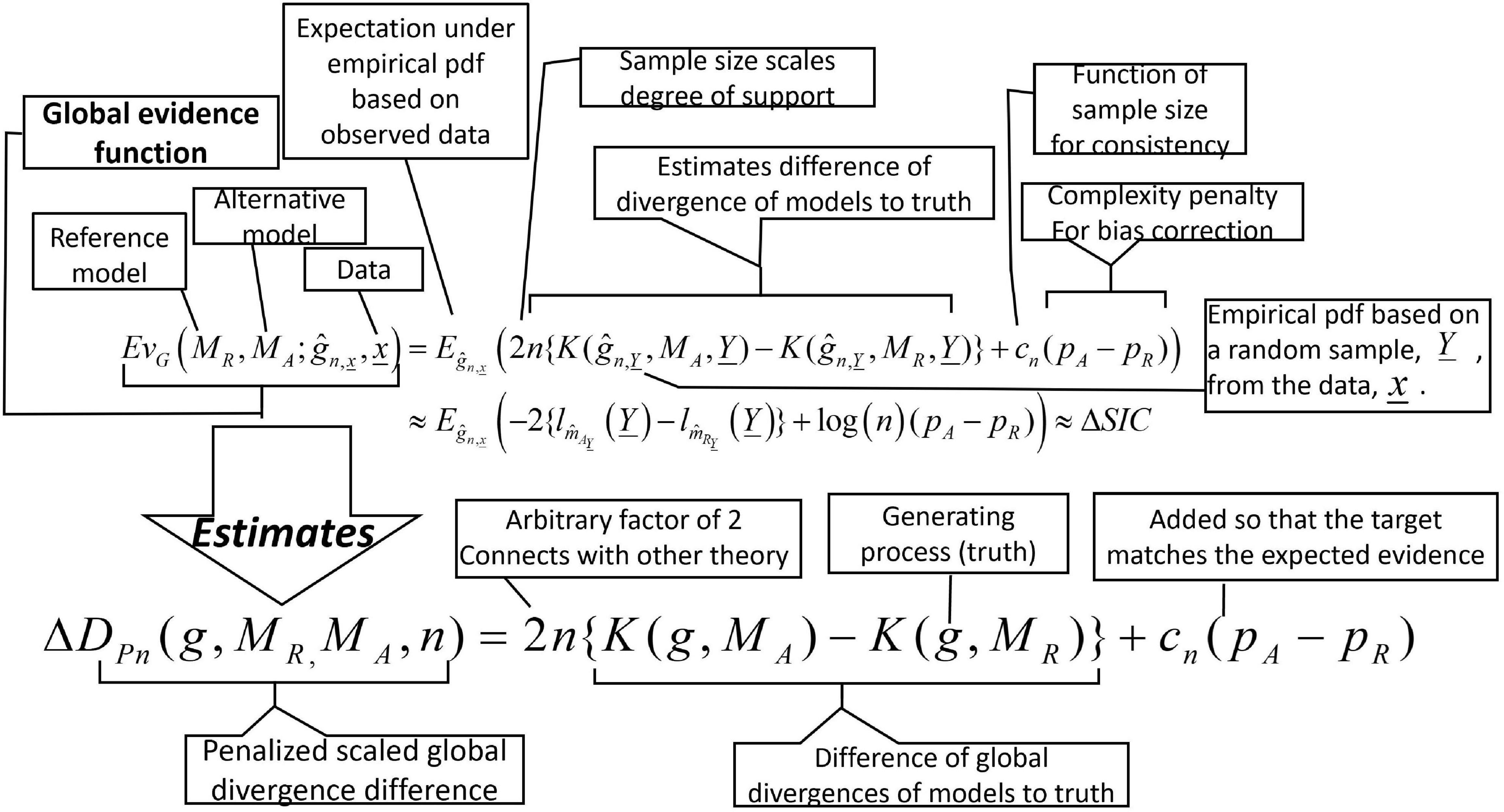
Figure 5. A schematic indicating how an evidence function relates to its global target. See supplement for a similar figure for local evidence. The principal differences between the figures are that for global evidence the target does not (and must not) depend on the data while for local evidence the target does (and must). Reflecting this difference, the global evidence function resamples the observed data to calculate likelihoods while the local does not.

We point out that, except for the nuance of kernel density smoothing, the algorithm we describe above for Ev_G is the EIC algorithm of Ishiguro et al. (1997) applied to ΔICs rather than directly to log-likelihoods. Kitagawa and Konishi (2010) point out that the bootstrap bias correction can be applied to any functional, not just the log-likelihood. The use of the expectation of the sampling distributions of ΔICs, which already contain an analytic bias correction, adds another layer of bias correction. Accordingly, the evidence should be 3rd order accurate (Kitagawa and Konishi, 2010).

Similarly, the local evidence function $E{v}_L(M_R,M_A;{\widehat{g}}_{n,\underset{¯}{x}},\underset{¯}{x})$ is an estimate of the local penalized scaled divergence difference, $\mathrm{\Delta }{d}_{Pn}(g_{n,\underset{¯}{X}},M_{R,}{M}_A,\underset{¯}{x})=E_{g_{n,\underset{¯}{X}}}\left(2n\{K(g_{n,\underset{¯}{Y}},M_A,\underset{¯}{x})-K(g_{n,\underset{¯}{Y}},M_R,\underset{¯}{x})\}+c_n(p_A-p_R)\right)$ (see Box 4 definition 22), and $E{v}_L(M_R,M_A;{\widehat{g}}_{n,\underset{¯}{x}},\underset{¯}{x})\approx E_{{\widehat{g}}_{n,\underset{¯}{x}}}\left(-2\{l_{{\widehat{m}}_{A_{\underset{¯}{Y}}}}\left(\underset{¯}{x}\right)-l_{{\widehat{m}}_{R_{\underset{¯}{Y}}}}\left(\underset{¯}{x}\right)\}+c_n(p_A-p_R)\right)$ (see Box 4 definition 24). The difference between the global and local is that in the calculation of the global evidence the observed data, $\underset{¯}{x}$, are considered as a realization of a random vector, $\underset{¯}{X}$, both in the estimation of the models to be compared and in the data on which they are compared. While in the local evidence, the data vector is considered random in the estimation of the models but fixed in the data on which they are compared.

It is well established in statistics that providing an estimate of an unknown quantity is not sufficient; one must provide uncertainty associated with such an estimate. We use aleatory probability to quantify this uncertainty (Lele, 2020a). In quantifying the pre-experiment uncertainty in evidence, we ask the question: How variable would the evidence be if we were to repeat the experiment? This is represented by the global (pre-experiment) sampling distribution of the evidence function. This distribution does not depend on the particular data set in hand.

When the competing models are fully specified and the reference model is the true model, Royall (1997, 2000) used the asymptotic Normal distribution of the LLR to approximate the sampling distribution of the evidence function and calculate the error probabilities. In Dennis et al. (2019), we derived the asymptotic distributions of the evidence function when the competing models are not fully specified and the true model is not part of the competing model spaces to approximate the sampling distribution and compute the error probabilities.

4.2. Uncertainty in Evidence

An important element common to all of our bootstrap procedures is that the complete evidence functions are the objects bootstrapped, not the component divergences. Thus, if the difference of information criterion values is the evidence function used, such a bootstrap will produce a single distribution of ΔICs rather than two distributions of IC values. This is necessary because the geometry of model misspecification (Dennis et al., 2019; Ponciano and Taper, 2019, see also Table 3) can create covariances (positive and negative) between the component divergences. These need to be captured by a bootstrap for it to accurately reflect the uncertainty in evidence. The non-parametric bootstrap method for the two cases described above is as follows.

TABLE 3

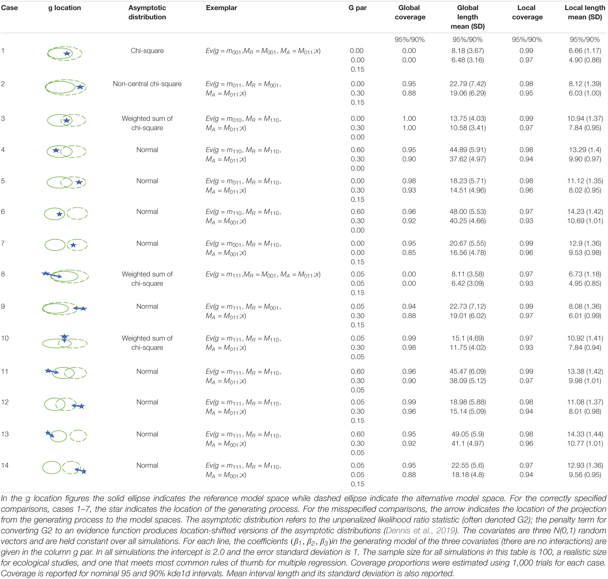
Table 3. The behavior of our global and local uncertainty procedures in all 14 possible model specification topologies.

4.2.1. Global Uncertainty in Evidence for the Fully Specified Models

Notice that in the bootstrap procedure in Section 4.1.1, we are bootstrapping the difference in the log-likelihood jointly and not each component separately. Evidence, innately, is a comparison between two quantities. Clearly uncertainty in evidence involves not just the variances of each component but also covariance between them. The uncertainty reflected in the bootstrap distribution accounts for the covariance also. Thus, if the two models are positively correlated with each other, the uncertainty is reduced whereas if they are negatively correlated, the uncertainty is higher than the sum of variances. This, thus, takes into account the geometry of the model spaces appropriately, even when the models are fully specified. The quantiles of the smoothed bootstrap density of $E{v}^{raw}(m_R,m_A;{\widehat{g}}_{n,\underset{¯}{x}},{\underset{¯}{x}}_b)$ give us confidence intervals for evidence (see Box 6 for an explicit algorithm).

4.2.2. Global Uncertainty in Evidence for Model Spaces With Unknown Parameter Values

Bootstrapping can also be used to obtain global confidence intervals for evidence with estimated parameters. The only difference is that the quantity bootstrapped is $E{v}_G^{raw}(M_{\text{R},}{M}_{\text{A}};{\widehat{g}}_{n,\underset{¯}{x}},{\underset{¯}{x}}_b)$, which is, in this paper, a difference of information criterion values (see Box 6 for an explicit algorithm).

4.2.3. Local Uncertainty in Evidence

Lele (2020a) reviewed the philosophical problems associated with global (pre-experiment) uncertainty and discussed the use of local (post-experiment) uncertainty in the context of linear regression. To recap, suppose we have only one covariate and we are fitting a linear regression through origin model. That is, the data are (x_i, y_i), i = 1, 2, …, n and we fit the model Y_i = βX_i + ε_i where $\mathrm{\epsilon }{}_i\sim N(0,{\mathrm{\sigma }}^2)$ are independent, identically distributed random variables. The maximum likelihood estimator of β is, $\widehat{\mathrm{\beta }}=\sum Y_i{X}_i\mathrm{/}\sum X_i^2$.

The question is: what is the variance of $\widehat{\mathrm{\beta }}$? If we consider the covariates to be random (this is the case when the experiment is not a designed experiment but an observational study), then $var(\widehat{\mathrm{\beta }})={\mathrm{\sigma }}^{2}E\left(1\mathrm{/}\sum X_i^2\right)$. If X_i∼N(0, 1), then $var(\widehat{\mathrm{\beta }})={\mathrm{\sigma }}^2/(n-2)$. This variance, which we term the global variance, is sometimes called an unconditional or pre-data variance. On the other hand, if we consider the covariates to be fixed, as is the case in designed experiments, $var(\widehat{\mathrm{\beta }}|x_{1,}{x}_2,\mathrm{\dots },x_n)={\mathrm{\sigma }}^2/\left\{\sum x_i^2\right\}$. This variance, which we call the local variance, is sometimes called the conditional or post-data variance.

The conditional variance is the variance most ecologists use when conducting regression analysis. Notice that conditional variance depends on the configuration of covariates the researcher observes in their particular data set. If the covariate values are highly dispersed, the slope is extremely well estimated; on the other hand, if the observed covariates values are not very different from each other, the slope is estimated with large uncertainty.

The local (conditional) variance makes intuitive sense: good data, strong inference; bad data, weak inference. It is argued (e.g., Goutis and Casella, 1995) that the global (unconditional) inference does not reflect this differentiated inferential value of the observed data appropriately. Even if the researcher happens to have good, dispersed covariates, the global variance does not recognize that happy event and increases the variance because the researcher, in another replication of the experiment could have observed less dispersed covariates and vice versa. We note that the pairwise resampling used in bootstrap inference for regression gives the unconditional variance and is robust against mean as well as error structure misspecification. On the other hand regression bootstrap based on residuals provides conditional inference but is only robust against error model misspecification (Efron and Tibshirani, 1993).

For local uncertainty, the sample space over which the variation is considered is a subset of the total sample space. This is called a “relevant subset” (Buehler, 1959). Such a relevant subset is often determined using an ancillary statistic. An ancillary statistic is a function of the data whose distribution does not depend on the parameters. There are, often, multiple ancillary statistics (Basu, 1964; Pena et al., 1992) and hence relevant subsets are not necessarily unique. In our opinion, the appropriateness of the relevant subset is determined based on the type of future experimental replication one envisions. Different future experiments determine different relevant subsets as was the case in the Mark-Capture-Recapture example in Box 2.

It has been argued that local (post-experiment, post-data, conditional) confidence intervals are preferable as the measure of uncertainty because they reflect the informativeness of the data at hand appropriately. If the data are highly informative, the local confidence intervals are shorter than the global confidence intervals and if the data are not informative, the local confidence intervals appropriately are wider than the global confidence intervals. Again, this argument hinges on the model being correctly specified.

Some august statisticians (e.g., Royall, 2004) argue the local interval is the only one that should be used irrespective of the design because design is an ancillary statistic and has no impact on the inference once the data are obtained. If the data are highly informative either by design or by chance, we should be quite confident about our estimate of the total population size, irrespective of what other experimenters might observe. It can be shown (see review in Lele, 2020b) that prediction of a new observation based on local uncertainty is more accurate than prediction based on global uncertainty. However, this result also depends on correct model specification.

On the other hand, other equally august statisticians (e.g., Cox, 2004 in his discussion of Royall, 2004) claim design should play a role in uncertainty quantification. We agree with this latter opinion on the importance of design. Both because the interpretation of uncertainty intervals should depend on the potential type of the future experimental replication, and thus so should the choice of the ancillary statistics or relevant subsets. And because, as we show in Section 5.2, the accuracy of the local interval depends on correct model specification to a greater degree than does the global.

4.2.4. Local Uncertainty When Comparing Two Model Spaces

Local evidence uncertainty in the comparison of model spaces is calculated similarly to global evidence uncertainty. Data sets are repeatedly reconstructed by bootstrapping the original data. With each bootstrapped, data set model parameters for both reference and alternative models are reestimated, and an evidence value comparing the models is calculated. The critical distinction between global and local uncertainty is that in the local calculations the likelihood for each bootstrapped model is evaluated using the original data not the bootstrapped data (see Box 6 for an explicit algorithm).

In Section 5, we use simulations to study the coverage properties of the global and local sampling distributions. Both the cases of linear regression and structural equation models are investigated.

5. Simulation Validation

If new statistical approaches are proposed, the scientific community has a legitimate expectation that they will be validated both mathematically, and computationally (Devezer et al., 2021). For a procedure that generates confidence intervals, whether global or local, to be a legitimate frequentist procedure, they need to cover/capture their targets at least at the specified level (Casella, 1992). The fundamental difference between global and local inference is that a global target cannot depend on the data at hand, while a local target must depend on the data at hand.

Globally we want our intervals to cover the global penalized scaled divergence difference: $\mathrm{\Delta }{D}_{Pn}(g_{n,\underset{¯}{X}},M_{R,}{M}_A,\underset{¯}{X})=E_{g_{n,\underset{¯}{X}}}\left(2n\{K(g_{n,\underset{¯}{Y}},M_A,\underset{¯}{Y})-K(g_{n,\underset{¯}{Y}},M_R,\underset{¯}{Y})\}+c_n(p_A-p_R)\right)$. Locally we want our intervals to cover the local penalized scaled divergence difference: $\mathrm{\Delta }{d}_{Pn}(g_{n,\underset{¯}{X}},M_{R,}{M}_A,\underset{¯}{x})=E_{g_{n,\underset{¯}{X}}}\left(2n\{K(g_{n,\underset{¯}{Y}},M_A,\underset{¯}{x})-K(g_{n,\underset{¯}{Y}},M_R,\underset{¯}{x})\}+c_n(p_A-p_R)\right)$. For the Kullback-Leibler divergence, this is approximately $-2\{l_{{\widehat{m}}_{A_{{\underset{¯}{x}}_b}}}\left(\underset{¯}{x}\right)-l_{{\widehat{m}}_{R_{{\underset{¯}{x}}_b}}}\left(\underset{¯}{x}\right)\}+c_n(p_A-p_R)$, the penalized scaled LLR for the observed data under the best approximating models in the two competing spaces to the true generating mechanism. We note this is identical to what is considered the target likelihood in the general profile likelihood literature, e.g., Section 3.1 of Pace and Salvan (2006).

5.1. Global and Local Coverages in Alternate Model Space Topologies

There are 14 possible topologies for a reference model space, an alternative model space and a generating process. The model spaces compared can be nested, overlapping, or disjoint. If the model comparison is correctly specified, the generating process will be in at least one of the model spaces. If the comparison is misspecified then the generating process will be in neither model space. Table 3 describes coverage and interval length for the global and local confidence intervals of the strength of evidence for model comparisons in each of these topologies in a simple multiple regression example (see the table legend for simulation details).

A number of interesting patterns can be observed in Table 3. In 12 of the 14 possible model space topologies, the global intervals cover reasonably, with actual coverages close to nominal coverages. Cases 1 and 8, however, have no coverage! Case 1 is the topology of nested models with the generating process in the reduced model. The asymptotic distribution for this case is chi-square. Case 8 represents the misspecified analog of Case 1, the approximating models are nested with the generating process closest to the reduced model. The asymptotic distribution for case 8 is a weighted sum of chi-square. This is a very flexible distribution, and in this case generates a distribution indistinguishable from a chi-square distribution. Alarm at this complete lack of coverage in these two cases is somewhat reduced by recognizing that the target ($\mathrm{\Delta }{D}_{Pn}(g,M_{R,}{M}_A,\underset{¯}{X})$) is the boundary of these chi-square distributions and hence impossible to capture with finite sampling.

On the other hand, the local confidence intervals for evidence behave well in all 14 possible model space topologies. In all cases local interval coverage exceeds the nominal levels. Overcovering is acceptable in approximate confidence intervals, particularly if interval length is narrow. In all cases of Table 1, the average lengths of the local intervals are less than that of global intervals. This is not always the case. For very small sample size, the average local interval length may exceed the average global interval length (see Figure 6).

FIGURE 6

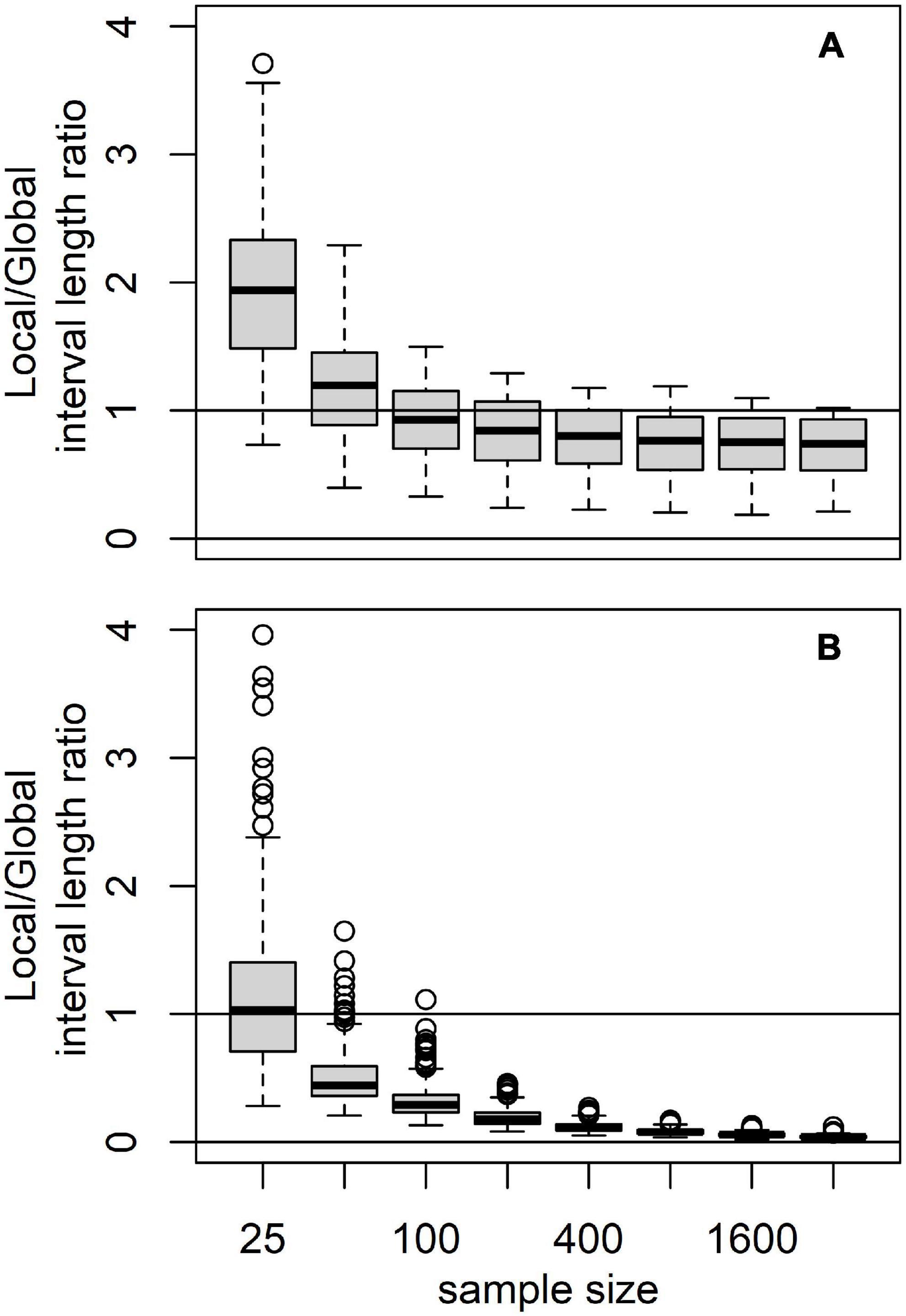
Figure 6. Box plots of the ratios of the local and global interval lengths as a function sample size. Each box summarizes the results for 1,000 simulations. In (A), all parameters (except for sample size) are set to those case 1 in Table 3. In (B), all parameters (except for sample size) are set to those of case 4 in Table 3.

5.2. Sample Size and Interval Lengths

In the linear models example of Table 3, global and local intervals respond quite differently to changes in sample size. These differences are explored in Figures 6, 7. Figure 6A shows box plots of the ratio of local interval length to global interval length over a range of increasing sample size for the case of case 1 from Table 1. The models compared are nested and the generating process is in the reduced model. The asymptotic distribution of evidence is chi-squared. At lower sample sizes the local interval length generally exceeds the global length. At higher sample sizes the local interval is generally shorter than the global interval, with the ratio appearing to approach a limit of at about 0.6. Model topologies shown in case 1 and 8 of Table 3 behave in this fashion.

FIGURE 7

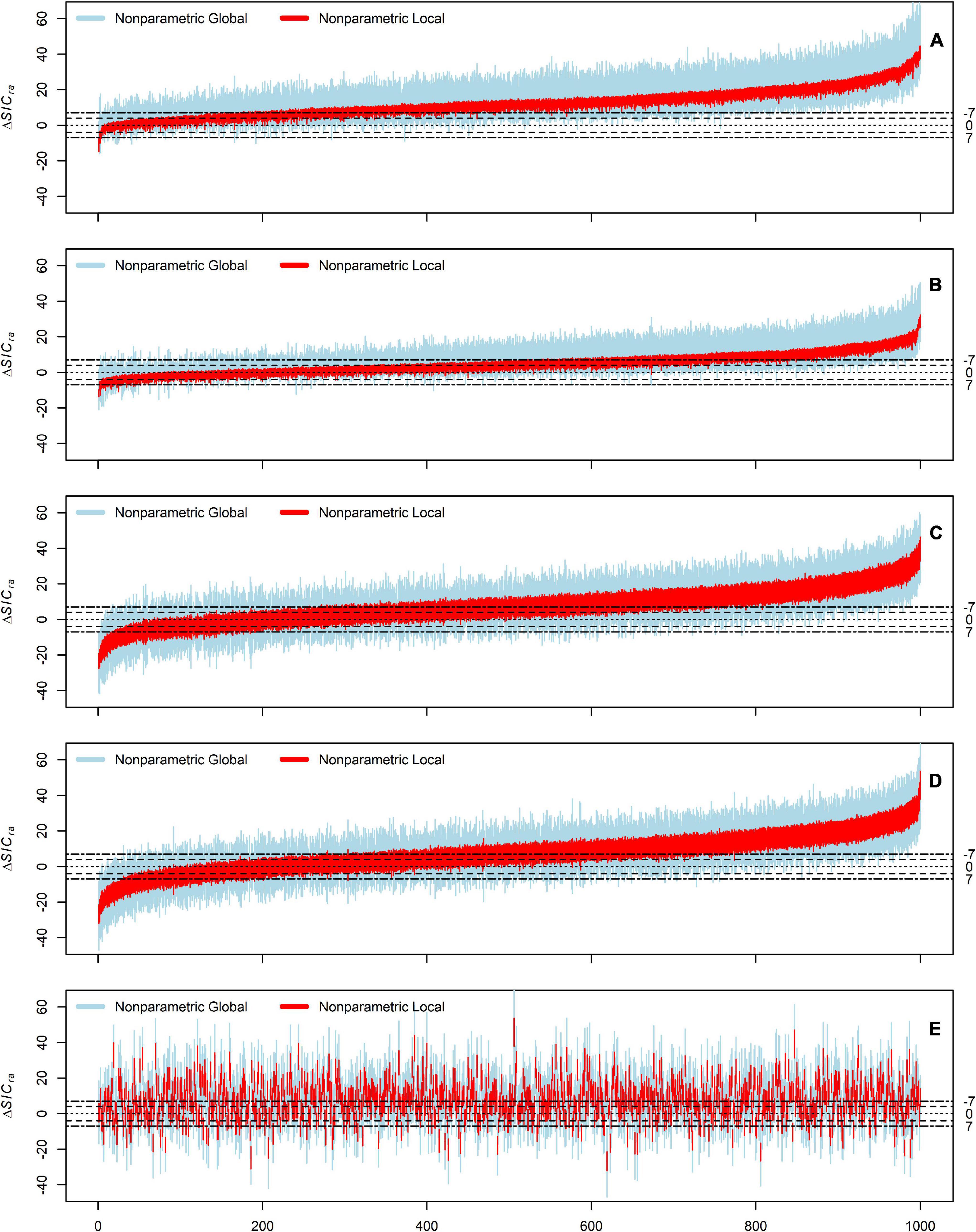
Figure 7. Global (blue) and local (red) 90% confidence intervals for the 1,000 simulations for cases (A–D) Described in the text. In (A–D) simulations are ordered by mean smoothed local evidence. Panel (E) presents the same data as (D) but ordered by the raw evidence. (A–C) Not shown reordered because with a Spearman correlation of ≥0.997 between raw and mean smoothed evidence in these cases, there is no perceptible change in the figures.

Figure 6B represents case 4 from Table 1. The models compared are overlapping with the generating process located in the non-overlapping portion of the reference model. The interval length behavior here is very different from that in panel A. Local intervals exceed global intervals only at the smallest sample sizes. Further, the local/global interval length ratio rapidly decreases toward 0 (rate $1\mathrm{/}\sqrt{n}$). All model topologies except those of cases 1 and 8 behave in this fashion.

For both global and local evidence, the expectation grows linearly with sample size. The standard deviation in global evidence grows as the square root of sample size. On the other hand, the standard deviation in local evidence approaches a constant as sample size increases (Kitagawa and Konishi, 2010). These differences have considerable impact on inference and experimental design.

The ability of the global interval to distinguish the observed evidence from 0 grows very slowly with sample size. On the other hand, the local interval will be able to detect real difference from 0 or either of our two thresholds with relatively small sample sizes. Nevertheless, in both global and local cases, the coefficient of variation in evidence goes to 0 as sample size grows to infinity.

5.3. Model Set Misspecification and Evidential Uncertainty

Here we demonstrate the effect of model set misspecification on the uncertainty of evidence with simulations based on the Grace and Keeley example. We look at four different conditions of model set adequacy: (A) correctly specified comparison with very strong evidence, (B) correctly specified comparison with strong evidence, (C) a mildly misspecified model comparison, and (D) a badly misspecified model comparison.

In case A), we compare the model that is the GKBM without the weakest path (GKBM – R∼L) with a model that is the GKBM without the second weakest path (GKBM – R∼C). The data in these simulations are generated from the estimated (GKBM – R∼L). The generating process is in the compared model set; therefore, the comparison is correctly specified.

In case B) we estimate and compare the same models as in case A. The generating model has same form as in case A (all the same paths are present) but one of the coefficients (R∼P) has been weakened from 0.299 to 0.205. The model set is still correctly specified, but the penalize divergence differences (whether global or local, see definitions 19 and 20) between the compared models is less than in case A. Consequently, the distribution of realized evidences (definitions 23 and 24) will be shifted to lower values.

Case C) compares the same models as in case A) {GKBM – R∼L, GKBM – R∼C}. The data are generated by the GKBM. Since the generating process (GKBM) is quite close to one of the models in the model set (GKBM – R∼L), the comparison is only mildly misspecified.

Finally, in case D) we compare a model that is the GKBM without the second strongest path (GKBM – C ∼ L) with a model that is the GKBM without the strongest path (GKBM – F ∼ A). As in case B), the data are generated by the GKBM. Since the generating process (GKBM) is quite different from both of the models in the model set, the comparison is badly misspecified.

Table 4 indicates that, at least in this example, under correct model specification, a researcher is very unlikely to obtain secure misleading evidence using either interval. On the other hand, the researcher is more likely to correctly obtain strong and secure evidence using the conditional interval than with the unconditional interval. If the model set is misspecified, secure misleading evidence becomes a possibility, and much more so using the conditional interval than the unconditional interval.

TABLE 4

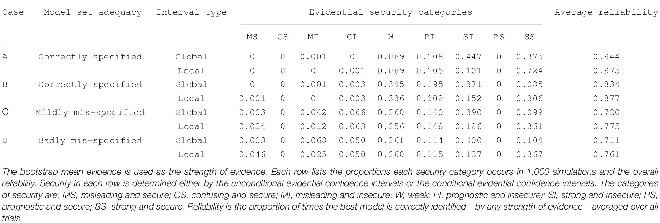
Table 4. Models compared and generating process for each model set are described in the text.

Interestingly, the average reliability (proportion of the time correct model is identified) is always slightly greater using the local evidence distribution rather than when using the global evidence distribution. This agrees with the previous results (Aitchison, 1975; Royall and Cumberland, 1985; Vidoni, 1995) that indicate predictive accuracy is greater using conditional inference.

The table gives the impression that there is little difference between mildly and badly misspecified model sets regarding evidence. But this is only because the choice of the mean of the smoothed bootstrapped ΔSIC as the measure of the strength of evidence rather than the raw ΔSIC has profound impact. Figure 7 presents the same data used to calculate Table 4 in another fashion. Here both the global and local intervals are explicitly plotted for each 1000 trials in the simulations of cases A, B, C, and D. The trials are sorted along the x axis by the mean smoothed bootstrapped strength of evidence. Panel E plots the same simulations and intervals as panel D, however, in this case the trials are sorted by the raw ΔSIC—not by the mean smoothed bootstrapped ΔSIC. We do not show plots with similar reordering for panels A, B, and C because in these cases the differences between the raw ΔSIC and the mean of the smoothed bootstrap are not visually perceptible.

In cases A, B, and C the difference between raw ΔSIC and smoothed mean bootstrapped ΔSIC are quite small and the correlation of raw ΔSIC and mean smoothed bootstrapped ΔSIC are greater than 0.99. Thus, there is almost no impact of choice of evidence measure in these cases with correct and mild misspecification. In the badly misspecified case D, there is a large average difference between raw ΔSIC and the mean smoothed bootstrapped ΔSIC and almost no correlation between them. Further, when using the raw ΔSIC, the location of the security intervals becomes almost unrelated to the strength of evidence. Consequently, the raw ΔSIC has almost no ability to securely identify the best model.

6. Discussion

Historically, the appeal of classical Neyman-Pearson testing has been the appearance of a strong control of error probabilities. Dennis et al. (2019) show this apparent control to be an illusion for the great majority of cases of interest in ecological science where models are misspecified. Under model misspecification, the realized error rate for a NP test can be less than or greater than its nominal rate. In some realistic cases the probability of error in a NP test can even increase with increasing sample size. Evidential analysis is superior to NP testing in that the total error rate always decreases with increasing sample size, both under correct model specification and under model misspecification.

However, Dennis et al. (2019) further points out that evidence is not entirely immune to problems due to model misspecification. Under misspecification, the probability of strong misleading evidence is not directly calculable because the generating process is not one of the models compared and is not even known. This current paper demonstrates that evidential error rates can be estimated even under model misspecification using non-parametric bootstrapping techniques (at least for independent data). Our approach to the bootstrapping of evidence differs from that used in the EIC (Konishi and Kitagawa, 1996; Ishiguro et al., 1997) in that we bootstrap the evidential comparison as a unit (see definitions 23 and 24 Box 4) whereas the EIC compares bootstrapped components. The joint bootstrapping allows us to estimate the impact of model set misspecification on evidential uncertainty more effectively. In this paper, we have only addressed the case of independently distributed data. We expect, however, that this approach can be extended to other data structures with the use of subtler bootstrapping methods (Lele, 1991, 2003; Lahiri, 2003).

It is important for scientists seeking to use and interpret these measures of uncertainty to understand the two intervals, global and local, are quantifying two different kinds of uncertainty. Statistical evidence is an estimate of the relationship between two models and the generating process. It is a penalized sample size scaled estimate of the difference of the divergences of two models from the generating process (truth). Valid confidence intervals of an estimate tell us how confident we are that the estimation target lies within the interval. In the global case, our estimate of evidence is the mean of the global bootstrap distribution of evidence, but the estimation target is the true penalized scaled divergence difference (Box 4, definition 19). In the local case our estimate of evidence is the mean of the local bootstrap distribution of evidence, but the target is the true evidence in the data without model estimation error (Box 4, definition 20).

For badly misspecified model comparisons local inference has strong and secure but misleading evidence more often than global inference. Nevertheless, we are in a position to make scientific inferences about the true relationships of our compared models to the generating process, backed by an uncertainty measure warrant.

Both the global and local evidence confidence intervals are important to science because they answer different questions. The global interval is a confidence interval on the true penalized scaled divergence difference. This speaks directly to the relative ability of our models to represent nature. The resampling is non-parametric to accommodate model misspecification. Further, the intervals incorporate both sample and model estimation uncertainty.

The global uncertainty we offer answers the question of how dissimilar to the current evidence we would expect new evidence to be if our experiment were to be repeated. This is the interval that other researchers should consider when trying to decide if their new results call the current results into question.

On the other hand, the local uncertainty tells you how confident you are in your evidence given the data you have collected. This might be the interval to use if you intend to take an action based on the results.

Replication is often seen as a pillar of science as a social activity (e.g., Johnson, 2002). But, what to replicate and how to measure is not always clearly understood. Which interval should a scientist use? Unfortunately, a univocal recommendation is not possible. The local interval is tremendously appealing because it is so short and because its overall reliability is greater (see Table 4). However, to justify inference based on it alone, the scientist needs to be able to defend the assumption of approximately correct model set specification. In the rough and tumble world of ecology this will rarely be possible, except for tightly controlled experiments with well understood error structures. The global interval presents an appraisal of the replicability of the scientist’s results. If the global interval has been presented, the local interval can be a useful indication of how good the results could possibly be. For the accumulation of understanding through science, the global interval may be preferable. This preference is grounded in our opening quote from Plato. Using the global interval, you will accept wrong statements less frequently than when using the local interval. However, in a decision context, where costs and benefits are explicit, the local inference’s property of making correct predictions more often than global inference might be important.

Hopefully, our recommendation to focus on the global interval will be only temporary. We expect that often model sets could be misspecified, but close enough to correctly specified that the local interval would be a justifiable improvement over the global interval. Research into diagnostics to identify these cases is called for (Cook and Weisberg, 1982). Useful diagnostics will involve more than measures of the adequacy of single models (e.g., Markatou and Sofikitou, 2019) they must somehow include measures of the geometry of the generating process and the competing models (Dennis et al., 2019; Ponciano and Taper, 2019).

In the meantime, little is practically lost. We agree with Goutis and Casella (1995) that “In any experiment both pre-data inferences and post-data inferences are important.” Our inferential strategy is a hybrid of local and global (conditional and unconditional). Our primary tool is the strength of evidence, which is local (i.e., conditional). The evidence expresses clearly what the data we have says about the relationships among nature and our models. Our secondary tools are our pair of measures of the security of the evidence. If we choose a global (that is unconditional measure) we gain an honest, if perhaps overly conservative, insight into the degree that chance, experimental/sample design, and model misspecification may have influenced our evidence. If we choose a local (that is a conditional measure) we gain a more precise understanding of the information in the data, at the risk of overconfidence due to model misspecification. Much of statistics both classical and Bayesian relies on conditional inference and thus might be over-confident in its conclusions in the face of potential model misspecification (see also Yang and Zhu, 2018).

While the global uncertainty, either calculated from asymptotic theory or from the non-parametric bootstrap is a useful statistic, it should not be interpreted too literally. As Fisher (1945a, b, 1955, 1956, 1960) long argued (see Rubin, 2020; Devezer et al., 2021 for detailed discussions) an exact repetition of an experiment is not possible in many branches of science. Certainly, this is true in ecology and environmental science, where heterogeneity and temporal data abound. To paraphrase Heraclitus, you can’t electrofish the same river twice. A more realistic understanding of global uncertainty would come from a metanalysis of the actual repetition of modestly sized experiments distributed in space and time than from a single large experiment. As an example, Jerde et al. (2019) conducts an evidential comparison of models for the intra-specific allometry of metabolic rate in fish using a database of 25 high quality studies, with 55 independent trials, across 16 fish species.

Jerde et al. (2019) use evidential support intervals in their analysis of the allometry of metabolic rate in fish. These intervals are post-data/conditional/local intervals. We wish to point out that, while both are useful, evidential support intervals and confidence intervals for evidence are different. Evidential support intervals indicate the range of parameter values in a model space that are not differentiated from the best estimate at a specified strength of evidence. Confidence intervals make a statement that at the specified probability a random interval, whose randomness stems from sample space probabilities, contains the true parameter value (Dennis, 2004). Under correct model specification, the support interval indicates over what range of parameter values the relative plausibility of the best estimate relative to the parameter value is less than the designated strength of evidence.

Under a correct model assumption, a ΔAIC interval is directly transformable into a confidence interval on the strength of evidence using Wilks-Wald hypothesis test inversion (see Dennis et al., 2019). The confidence level of this transformed interval will depend only on the chosen strong evidence threshold, k_R. On the other hand, the level of an evidence confidence interval corresponding to a ΔSIC interval will be a function of both k_R and log(n). As n increases the confidence level will increase. This parametric confidence interval is preferred if a true model assumption is justified. Using a nonparametric confidence interval rather than a evidence interval acknowledges that your model set may be misspecified.

Global and local confidence intervals for the strength of evidence, at least as we have developed them in this paper, are used in the comparisons of model spaces. The intervals discussed are on the space of strength of evidence values; they are not on the space of parameter values nor are they on the space of predictions. We have seen that the interpretation of local and global intervals on evidence requires deep consideration of the scientific questions being asked. Complexities also arise for conditional and unconditional intervals for parameters and for predictions. We defer to another paper a unified discussion of the effects of post-data and pre-data intervals on science.

As laid out in Royall (1997) and Dennis et al. (2019), one of the great strengths of the evidential approach relative to NPHT, is that M, the probability of misleading evidence goes to 0 as sample size increases whereas α, the corresponding uncertainty measure in NPHT, remains constant. It is a commonplace in introductory mathematical statistics courses that hypothesis tests and confidence intervals are inter-convertible. Given this, a reasonable question to ask is: By incorporating confidence intervals have we somehow given up the superior error structure of evidence? The answer to this question is no. The NPHT freights both its measure of the strength of evidence and its measure of uncertainty onto α. We use 2 measures; the primary is evidence and as sample size increases this will go to either + ∞ or −∞. Our second measure is the standard deviation of evidence and, as discussed in Section 5.2, this does not grow as rapidly as the evidence itself. As a consequence, the probability of making an error of assignment—at any specified level of confidence—also goes to 0 as sample size increases.

A literature has developed that constructs confidence sets (i.e., confidence intervals on discrete parameters) in model identification (Hansen et al., 2011; Ferrari and Yang, 2015; Sayyareh, 2017; Li et al., 2019; Zheng et al., 2019; Liu et al., 2021). These papers differ from the current work in several important fashions. First, the confidence intervals being considered are not even related. Our work constructs a confidence interval on a continuous parameter, the strength of evidence between models. The parameter in the model confidence sets literature is a discrete parameter of model inclusion. Second, one feature of the confidence set approach is that specification of the entire model set is essential to interpretation of a confidence set. This is a drawback that is shared by Bayesian model selection and model averaging.

Our worked example in Section 3 makes 14 evidential comparisons. Should some sort of adjustment be made? If the analyst is willing to specify the model set, multiple comparison adjustments are appropriate in evidential comparisons, particularly when massive numbers of comparisons or badly misspecified model sets are involved. Fortunately, there are several features of the evidential paradigm that allow it to respond to multiple comparisons with more grace and less cost than classical hypothesis testing approaches. Evidential multiple comparisons have been extensively discussed in Strug and Hodge (2006a,b) and Taper and Lele (2011). These reviews were written from the standpoint of correctly specified model sets with the probability of misleading evidence being estimated by Royall’s universal bound (Royall, 1997). We hope to soon write a paper on evidential multiple comparisons that utilizes the ability of our non-parametric bootstrap to estimate the probability of misleading evidence in the face of model misspecification (Taper et al., 2019; Liu et al., 2021).

Another attribute of the model confidence set papers is that they all make their selections based on some form of NPHT. We suspect that these confidence sets inherit the stringent properties of multiple comparisons in NPHTs rather than the more permissive properties of evidential multiple comparison. We look forward to investigating this in more detail in the future.

Due to limitations of space, the topic of this paper is treated strictly as a development of evidentialist statistics using a frequentist notion of probability. When epistemic comparisons are made, they are to NPHT. Readers interested in better understanding the relative epistemic character of evidential statistics, error statistics (classical hypothesis testing), and Bayesian statistics might explore some of Dennis (2004), Lele (2004a,b, 2010, 2020a), Taper and Lele (2004), Efron (2005), Lele and Allen (2006), Lele et al. (2007, 2010), Lele and Dennis (2009), Ponciano et al. (2009, 2012), Bandyopadhyay and Forster (2011), Bandyopadhyay et al. (2016), Taper and Ponciano (2016), Mayo (2018), and Brittan and Bandyopadhyay (2019) as examples of a vast battleground of literature on the topic.

7. Conclusion

Neither the Bayesian nor classical frequentist statistical toolkits appear adequate for the increasingly complex challenges of the future. In the long run, neither our models nor our data, nor our conclusions are static. We need to look at multiple models realizing that we do not know truth and evolve these models toward better approximations of truth with the accumulation of data and use of evidence as a selection function.

We have produced both global and local uncertainty measures that are easily calculated for many analyses using the R-code that we supply in Supplementary Material. Further, by creating three categories for the strength of evidence coupled with three categories for the security of evidence we have constructed a conceptual language that allows scientists a statistically valid way to talk, and publish, about interesting results that are not yet conclusive.

Data Availability Statement

The original contributions presented in the study are included in the article/Supplementary Material, further inquiries can be directed to the corresponding author/s.

Author Contributions

MT wrote the R Code. MT and SL jointly wrote the first draft. All authors contributed to the many draft revisions and conceived of this study jointly.

Funding

MT, SL, BD, and JP were all partially funded by a grant from the Japan Society for the Promotion of Science to Professor Ichiro Ken Shimatani. JP was partially supported by two grants from the US National Institute of Health grant number to University of Florida NIH R01 GM103604 to JP and NIH 1R01GM117617 to Profs. Jason K. Blackburn and J. M. Ponciano. The participation of CJ in this research was partially funded by USAID (AID-OAA-A-00057), NASA (NNX14AR62A), BOEM (MC15AC00006), and NOAA’s support of the Santa Barbara Channel Marine Biodiversity Observation Network.

Conflict of Interest

The authors declare that the research was conducted in the absence of any commercial or financial relationships that could be construed as a potential conflict of interest.

Publisher’s Note

All claims expressed in this article are solely those of the authors and do not necessarily represent those of their affiliated organizations, or those of the publisher, the editors and the reviewers. Any product that may be evaluated in this article, or claim that may be made by its manufacturer, is not guaranteed or endorsed by the publisher.

Acknowledgments

Dr. James B. Grace kindly contributed the original data set from Grace and Keeley (2006). Drs. Prasanta Bandyopadhyay, James B. Grace, Jake M. Ferguson, and David Staples all read the manuscript carefully and provided many helpful discussions and comments. The editor, IS, and three reviewers provided comments that greatly improved the manuscript.

Supplementary Material

The files KKICv.R, KKICv.demo.R, GK.d.rds, and README.md can be found at https://github.com/jmponciano/mltaper-bootstrap.

Supplementary Figure 1 | A schematic indicating how a local evidence function relates to its target. See the manuscript body for a similar figure for global evidence. The principal differences between the figures are that for global evidence the target does not (and must not) depend on the data while for local evidence the target does (and must). Reflecting this difference, the global evidence function resamples the observed data to calculate likelihoods while the local does not.

Footnotes

1. ^ The SIC is frequently referred to as the BIC or Bayesian Information Criterion. Since we use the criterion as one of a series of criteria, all with frequentist derivations (Nishii, 1988) we use the notation SIC to avoid Bayesian implications.
2. ^ As voiced by the character Hector Barbossa https://www.youtube.com/watch?v=6GMkuPiIZ2k&ab_channel=JesseDB

References

Aitchison, J. (1975). Goodness of prediction fit. Biometrika 62, 547–554.

Google Scholar

Akaike, H. (1973). “Information theory as an extension of the maximum likelihood principle,” in Second International Symposium on Information Theory, eds B. N. Petrov and F. Csaki (Budapest: Akademiai Kiado).

Google Scholar

Anderson, D. R. (2008). Model Based Inference in the Life Sciences: a Primer on Evidence. Berlin: Springer Science & Business Media.

Google Scholar

Bandyopadhyay, P. S., Brittan, G., and Taper, M. L. (2016). Belief, Evidence, and Uncertainty: Problems of Epistemic Inference. Berlin: Springer.

Google Scholar

Bandyopadhyay, P. S., and Forster, M. R. (eds) (2011). Philosophy of Statistics. Amsterdam: Elsevier.

Google Scholar

Barnard, G. A. (1949). Statistical inference. J. R. Statist. Soc. Series B-Statistical Methodol. 11, 115–149.

Google Scholar

Basu, D. (1964). Recovery of ancillary information. Sankhya 26, 3–16.

Google Scholar

Birnbaum, A. (1962). On foundations of statistical-inference. J. Am. Statist. Assoc. 57, 269–306.

Google Scholar

Birnbaum, A. (1970). Statistical methods in scientific inference. Nature 225:1033.

Google Scholar

Birnbaum, A. (1972). More on concepts of statistical evidence. J. Am. Statist. Assoc. 67, 858–861.

Google Scholar

Bollen, K. A. (1989). Structural Equations with Latent Variables. New York, NY: Wiley.

Google Scholar

Bollen, K. A., and Pearl, J. (2013). “Eight myths about causality and structural equation models,” in Handbook of causal analysis for social research, ed. L. Morgan Stephen (Dordrecht: Springer).

Google Scholar

Breitsohl, H. (2019). Beyond ANOVA: an introduction to structural equation models for experimental designs. Organ. Res. Methods 22, 649–677. doi: 10.1016/j.addbeh.2018.08.030

PubMed Abstract | CrossRef Full Text | Google Scholar

Brittan, G., and Bandyopadhyay, P. S. (2019). Ecology, evidence, and objectivity: in search of a bias-free methodology. Front. Ecol. Evol. 7:399. doi: 10.3389/fevo.2019.00399

CrossRef Full Text | Google Scholar

Bruckheimer, J., and Verbinski, G. (2003). Pirates of the Caribbean: The Curse of the Black Pearl. Burbank, CA: Walt Disney Pictures.

Google Scholar

Buehler, R. ‘J. (1959). Some validity criteria for statistical inferences. Ann. Mathematical Statist. 30, 845–863.

Google Scholar

Burnham, K. P., and Anderson, D. R. (2002). Model Selection and Multi-model Inference: A Practical Information-Theoretic Approach, 2nd Edn. New York, NY: Springer-Verlag.

Google Scholar

Casella, G. (1992). Conditional inference from confidence sets. Lecture Notes-Monograph Series 17, 1–12.

Google Scholar

Casella, G., and Berger, R. L. (2002). Statistical Inference, 2nd Edn. Boston, MA: Cenage Learning.

Google Scholar

Cheng, C. L., and Van Ness, J. W. (1999). Statistical Regresion with Measurement Error, 1st Edn. London: Arnold.

Google Scholar

Cook, R. D., and Weisberg, S. (1982). Residuals and Influence in Regression. London: Chapman and Hall.

Google Scholar

Cooper, L. N., Lee, A. H., Taper, M. L., and Horner, J. R. (2008). Relative growth rates of predator and prey dinosaurs reflect effects of predation. Proc. R. Soc. B-Biol. Sci. 275, 2609–2615. doi: 10.1098/rspb.2008.0912

PubMed Abstract | CrossRef Full Text | Google Scholar

Cox, D. R. (1958). Planning of Experiments. Oxford: Wiley.

Google Scholar

Cox, D. R. (2004). “Commentary on the likelihood paradigm for statistical evidence by R. Royall,” in The Nature of Scientific Evidence: Statistical, Philosophical and Empirical Considerations, eds M. L. Taper and S. R. Lele (Chicago, ILL: University of Chicago Press).

Google Scholar

Cox, D. R., and Reid, N. (1987). Parameter orthogonality and approximate conditional inference. J. R. Statist. Soc. Series B (Methodological) 49, 1–39.

Google Scholar

De Blasi, P., and Schweder, T. (2018). Confidence distributions from likelihoods by median bias correction. J. Statist. Plann. Inference 195, 35–46.

Google Scholar

Dennis, B. (2004). “Statistics and the scientific method in ecology,” in The Nature of Scientific Evidence: Statistical, Philosophical and Empirical Considerations, eds M. L. Taper and S. R. Lele (Chicago, ILL: The University of Chicago Press).

Google Scholar

Dennis, B., Ponciano, J. M., Taper, M. L., and Lele, S. R. (2019). Errors in statistical inference under model misspecification: evidence, hypothesis testing, and AIC. Front. Ecol. Evol. 7:372. doi: 10.3389/fevo.2019.00372

PubMed Abstract | CrossRef Full Text | Google Scholar

Devezer, B., Navarro, D. J., Vandekerckhove, J., and Buzbas, E. O. (2021). The case for formal methodology in scientific reform. R. Soc. Open Sci. 8:200805. doi: 10.1098/rsos.200805

PubMed Abstract | CrossRef Full Text | Google Scholar

Edwards, A. W. F. (1992). Likelihood. Expanded Edition. Cambridge: Cambridge University Press.

Google Scholar

Efron, B. (2005). Bayesians, frequentists, and scientists [Editorial Material]. J. Am. Statist. Assoc. 100, 1–5. doi: 10.1198/01621450500000033

PubMed Abstract | CrossRef Full Text | Google Scholar

Efron, B., and Tibshirani, R. (1993). An Introduction to the Bootstrap. London: Chapman and Hall.

Google Scholar

Ferrari, D., and Yang, Y. H. (2015). Confidence sets for model selection by F-testing. Statistica Sinica 25, 1637–1658. doi: 10.5705/ss.2014.110

PubMed Abstract | CrossRef Full Text | Google Scholar

Fieberg, J. R., Vitense, K., and Johnson, D. H. (2020). Resampling-based methods for biologists. Peerj 8:e908.

Google Scholar

Fisher, R. (1955). Statistical methods and scientific induction. J. R. Statist. Soc. Series B-Statist. Methodol. 17, 69–78.

Google Scholar

Fisher, R. A. (1922). On the mathematical foundations of theoretical statistics. Philos. Trans. R. Soc. London Series A 222, 309–368.

Google Scholar

Fisher, R. A. (1936). Uncertain inference. Sci. Monthly 43, 402–410.

Google Scholar

Fisher, R. A. (1945a). A new test for 2X2 tables. Nature 156, 388–388.

Google Scholar

Fisher, R. A. (1945b). The logical inversion of the notion of the random variable. Sankhya 7, 129–132.

Google Scholar

Fisher, R. A. (1956). Statistical Methods and Scientific Inference. London: Oliver and Boyd.

Google Scholar

Fisher, R. A. (1960). Scientific thought and the refinement of human reasoning. J. Operat. Res. Soc. Japan 3, 1–10.

Google Scholar

Geenens, G., and Wang, C. (2018). Local-Likelihood transformation kernel density estimation for positive random variables. J. Computat. Graph. Statist. 27, 822–835.

Google Scholar

Godambe, V. P. (1960). An optimum property of regular maximum-likelihood estimation. Ann. Mathematical Stat. 31, 1208–1211.

Google Scholar

Goutis, C., and Casella, G. (1995). Frequentist post-data inference. Int. Statist. Rev. 63, 325–344. doi: 10.1890/13-1291.1

PubMed Abstract | CrossRef Full Text | Google Scholar

Grace, J. B. (2008). Structural equation modeling for observational studies. J. Wildlife Manag. 72, 14–22.

Google Scholar

Grace, J. B., Anderson, T. M., Olff, H., and Scheiner, S. M. (2010). On the specification of structural equation models for ecological systems. Ecol. Monographs 80, 67–87.

Google Scholar

Grace, J. B., and Bollen, K. A. (2008). Representing general theoretical concepts in structural equation models: the role of composite variables. Environ. Ecol. Statist. 15, 191–213.

Google Scholar

Grace, J. B., and Irvine, K. M. (2020). Scientist’s guide to developing explanatory statistical models using causal analysis principles. Ecology 101:e02962. doi: 10.1002/ecy.2962

PubMed Abstract | CrossRef Full Text | Google Scholar

Grace, J. B., and Keeley, J. E. (2006). A structural equation model analysis of postfire plant diversity in California shrublands. Ecol. Appl. 16, 503–514. doi: 10.1890/1051-0761(2006)016[0503:asemao]2.0.co;2

CrossRef Full Text | Google Scholar

Grace, J. B., and Pugesek, B. H. (1997). A structural equation model of plant species richness and its application to a coastal wetland. Am. Nat. 149, 436–460.

Google Scholar

Grace, J. B., Youngblood, A., and Scheiner, S. M. (2009). “Structural equation modeling and ecological experiments,” in Real World Ecology: Large-Scale and Long-Term Case Studies and Methods, eds S. Miao, S. Carstenn, and M. Nungesser (Berlin: Springer Science).

Google Scholar

Hacking, I. (1965). Logic of Statistical Inference. Cambridge: Cambridge University Press.

Google Scholar

Hall, P. (1986). On the bootstrap and confidence-intervals. Ann. Statist. 14, 1431–1452.

Google Scholar

Hall, P. (1987). On the bootstrap and likelihood-based confidence-regions. Biometrika 74, 481–493.

Google Scholar

Halsey, L. G. (2019). The reign of the p-value is over: what alternative analyses could we employ to fill the power vacuum? Biol. Lett. 15:20190174. doi: 10.1098/rsbl.2019.0174

PubMed Abstract | CrossRef Full Text | Google Scholar

Hansen, P. R., Lunde, A., and Nason, J. M. (2011). The model confidence set. Econometrica 79, 453–497. doi: 10.3982/ecta5771

PubMed Abstract | CrossRef Full Text | Google Scholar

Holland, S. M. (2019). Estimation, not significance. Paleobiology 45, 1–6.

Google Scholar

Hurvich, C. M., and Tsai, C. L. (1989). Regression and time-series model selection in small samples. Biometrika 76, 297–307.

Google Scholar

Ishiguro, M., Sakamoto, Y., and Kitagawa, G. (1997). Bootstrapping log likelihood and EIC, an extension of AIC. Ann. Institute Statist. Mathematics 49, 411–434. doi: 10.1111/1541-0420.00020

PubMed Abstract | CrossRef Full Text | Google Scholar

Jerde, C. L., Kraskura, K., Eliason, E. J., Csik, S., Stier, A. C., and Taper, M. L. (2019). Strong evidence for an intraspecific metabolic scaling coefficient near 0.89 in fish. Front. Physiol. 10:1166. doi: 10.3389/fphys.2019.01166

PubMed Abstract | CrossRef Full Text | Google Scholar

Johnson, D. H. (1999). The insignificance of statistical significance testing. J. Wildlife Manag. 63, 763–772.

Google Scholar

Johnson, D. H. (2002). The importance of replication in wildlife research. J. Wildlife Manag. 66, 919–932.

Google Scholar

Keeley, J. E., Baer-Keeley, M., and Fotheringham, C. J. (2005). Alien plant dynamics following fire in mediterranean-climate California shrublands. Ecol. Appl. 15, 2109–2125.

Google Scholar

Keeley, J. E., Brennan, T., and Pfaff, A. H. (2008). Fire severity and ecosytem responses following crown fires in California shrublands. Ecol. Appl. 18, 1530–1546. doi: 10.1890/07-0836.1

CrossRef Full Text | Google Scholar

Kitagawa, G., and Konishi, S. (2010). Bias and variance reduction techniques for bootstrap information criteria. Ann. Institute Statistical Mathemat. 62:209.

Google Scholar

Konishi, S., and Kitagawa, G. (1996). GeneralisedGeneralized information criteria in model selection. Biometrika 83, 875–890.

Google Scholar

Konishi, S., and Kitagawa, G. (2008). Information Criteria and Statistical Modeling. New York, NY: Springer.

Google Scholar

Lahiri, S. N. (2003). Resampling Methods for Dependent Data. New York, NY: Springer.

Google Scholar

Laughlin, D. C., and Grace, J. B. (2019). Discoveries and novel insights in ecology using structural equation modeling. Ideas Ecol. Evol. 12, 28–34.

Google Scholar

Lele, S. (1991). Jackknifing linear estimating equations - asymptotic theory and applications in stochastic-processes. J. R. Statist. Soc. Series B-Methodol. 53, 253–267.

Google Scholar

Lele, S. R. (2003). Impact of bootstrap on the estimating functions. Statist. Sci. 18, 185–190.

Google Scholar

Lele, S. R. (2004a). “Elicit data, not prior: on using expert opinion in ecological studies,” in The Nature of Scientific Evidence: Statistical, Philosophical and Empirical Considerations, eds M. L. Taper and S. R. Lele (Chicago, ILL: University of Chicago Press).

Google Scholar

Lele, S. R. (2004b). “Evidence functions and the optimality of the law of likelihood,” in The Nature of Scientific Evidence: Statistical, Philosophical and Empirical Considerations, eds M. L. Taper and S. R. Lele (Chicago, ILL: The University of Chicago Press).

Google Scholar

Lele, S. R. (2010). Model complexity and information in the data: could it be a house built on sand? Ecology 91, 3493–3496. doi: 10.1890/10-0099.1

CrossRef Full Text | Google Scholar

Lele, S. R. (2020a). Consequences of lack of parameterization invariance of non-informative Bayesian analysis for wildlife management: survival of San Joaquin kit fox and declines in amphibian populations. Front. Ecol. Evol. 7:501. doi: 10.3389/fevo.2019.00501

CrossRef Full Text | Google Scholar

Lele, S. R. (2020b). How should we quantify uncertainty in statistical inference? Front. Ecol. Evol. 8:35. doi: 10.3389/fevo.2020.00035

CrossRef Full Text | Google Scholar

Lele, S. R., and Allen, K. L. (2006). On using expert opinion in ecological analyses: a frequentist approach. Environmetrics 17, 683–704. doi: 10.1002/env.786

CrossRef Full Text | Google Scholar

Lele, S. R., and Dennis, B. (2009). Bayesian methods for hierarchical models: are ecologists making a Faustian bargain? Ecol. Appl. 19, 581–584. doi: 10.1890/08-0549.1

CrossRef Full Text | Google Scholar

Lele, S. R., Dennis, B., and Lutscher, F. (2007). Data cloning: easy maximum likelihood estimation for complex ecological models using Bayesian Markov chain Monte Carlo methods. Ecol. Lett. 10, 551–563. doi: 10.1111/j.1461-0248.2007.01047.x

PubMed Abstract | CrossRef Full Text | Google Scholar

Lele, S. R., Nadeem, K., and Schmuland, B. (2010). Estimability and likelihood inference for generalized linear mixed models using data cloning. J. Am. Statist. Assoc. 105, 1617–1625.

Google Scholar

Lele, S. R., and Taper, M. L. (2012). “Information criteria in ecology,” in Encyclopedia of Theoretical Ecology, eds A. Hastings and L. Gross (Berkeley: University of California Press).

Google Scholar

Li, Y., Luo, Y. T., Ferrari, D., Hu, X. N., and Qin, Y. C. (2019). Model confidence bounds for variable selection. Biometrics 75, 392–403. doi: 10.1111/biom.13024

PubMed Abstract | CrossRef Full Text | Google Scholar

Lindsay, B. G. (2004). “Statistical distances as loss functions in assessing model adequacy,” in The Nature of Scientific Evidence: Statistical, philosophical and Empirical Considerations, eds M. L. Taper and S. R. Lele (Chicago, ILL: University of Chicago Press). doi: 10.3390/e20060464

PubMed Abstract | CrossRef Full Text | Google Scholar

Linhart, H. (1988). A test whether 2 AICs differ significantly. South African Statist. J. 22, 153–161.

Google Scholar

Liu, X. H., Li, Y. Y., and Jiang, J. M. (2021). Simple measures of uncertainty for model selection. Test 30, 673–692.

Google Scholar

Markatou, M., and Sofikitou, E. M. (2019). Statistical distances and the construction of evidence functions for model adequacy. Front. Ecol. Evol. 7:447447. doi: 10.3389/fevo.2019.00447447

CrossRef Full Text | Google Scholar

Mayo, D. G. (2018). Statistical Inference as Severe Testing. Cambridge: Cambridge University Press.

Google Scholar

Meeker, W. Q., and Escobar, L. A. (1995). Teaching about approximate confidence-regions based on maximum-likelihood-estimation. Am. Statist. 49, 48–53.

Google Scholar

Nagler, T., and Vatter, T. (2019). kde1d: Univariate Kernel Density Estimation. R Package Version 1.0.2. Available online at: https://CRAN.R-project.org/package=kde1d

Google Scholar

Neyman, J. (1937). Outline of a theory of statistical estimation based on the classical theory of probability. Philos. Trans. R. Soc. London Series A Mathemat. Phys. Sci. 236, 333–380.

Google Scholar

Neyman, J., and Pearson, E. S. (1933). On the problem of the most efficient tests of statistical hypotheses. Philos. Trans. R. Soc. London Series A 231, 289–337.

Google Scholar

Ng, C. T., and Joe, H. (2016). Comparison of non-nested models under a general measure of distance. J. Statist. Plann. Inference 170, 166–185. doi: 10.1016/j.jspi.2015.10.004

CrossRef Full Text | Google Scholar

Nishii, R. (1988). Maximum-Likelihood principle and model selection when the true model is unspecified. J. Multivariate Anal. 27, 392–403.

Google Scholar

Pace, L., and Salvan, A. (2006). Adjustments of the profile likelihood from a new perspective. J. Statist. Plann. Inference 136, 3554–3564.

Google Scholar

Pawitan, Y. (2001). In All Likelihood: Statistical Modeling and Inference Using Likelihood. Oxford: Oxford University Press.

Google Scholar

Pena, E. A., Rohatgi, V. K., and Szekely, G. J. (1992). On the non-existence of ancillary statistics. Statist. Probab. Lett. 15, 357–360.

Google Scholar

Pierce, D. A., and Bellio, R. (2017). Modern likelihood-frequentist inference. Int. Statist. Rev. 85, 519–541.

Google Scholar

Ponciano, J. M., Burleigh, G., Braun, E. L., and Taper, M. L. (2012). Assessing parameter identifiability in phylogenetic models using data cloning. Systematic Biol. 61, 955–972. doi: 10.1093/sysbio/sys055

PubMed Abstract | CrossRef Full Text | Google Scholar

Ponciano, J. M., and Taper, M. L. (2019). Model projections in model space: a geometric interpretation of the AIC allows estimating the distance between truth and approximating models. Front. Ecol. Evol. 7:413. doi: 10.3389/fevo.2019.00413

PubMed Abstract | CrossRef Full Text | Google Scholar

Ponciano, J. M., Taper, M. L., Dennis, B., and Lele, S. R. (2009). Hierarchical models in ecology: confidence intervals, hypothesis testing, and model selection using data cloning. Ecology 90, 356–362. doi: 10.1890/08-0967.1

CrossRef Full Text | Google Scholar

Powell, L. A., and Gale, G. A. (2015). Estimation of Parameters for Animal Populations: a Primer for the Rest of US. Lincoln, NE: Caught Napping Publications.

Google Scholar

Royall, R. M. (1997). Statistical Evidence: a Likelihood Paradigm. London: Chapman & Hall.

Google Scholar

Royall, R. M. (2000). On the probability of observing misleading statistical evidence. J. Am. Statist. Assoc. 95, 760–780.

Google Scholar

Royall, R. M. (2004). “The likelihood paradigm for statistical evidence,” in The Nature of Scientific Evidence: Statistical, Philosophical and Empirical Considerations, eds M. L. Taper and S. R. Lele (Chicago, ILL: The University of Chicago Press).

Google Scholar

Royall, R. M., and Cumberland, W. G. (1985). Conditional coverage properties of finite population confidence-intervals. J. Am. Statist. Assoc. 80, 355–359. doi: 10.1093/jssam/smv031

PubMed Abstract | CrossRef Full Text | Google Scholar

Rubin, M. (2020). Repeated sampling from the same population? a critique of Neyman and Pearson’s responses to Fisher. Eur. J. Philos. Sci. 10:42.

Google Scholar

Sayyareh, A. (2017). Non parametric multiple comparisons of non nested rival models. Commun. Statistics-Theory Methods 46, 8369–8386. doi: 10.1080/03610926.2016.1179759

CrossRef Full Text | Google Scholar

Sayyareh, A., Obeidi, R., and Bar-Hen, A. (2011). Empiricial comparison between some model selection criteria. Commun. Statistics-Simulat. Comput. 40, 84–98. doi: 10.1080/03610918.2010.530367

CrossRef Full Text | Google Scholar

Schwarz, G. (1978). Estimating the dimension of a model. Ann. Statist. 6, 461–464. doi: 10.1007/978-3-319-10470-6_18

CrossRef Full Text | Google Scholar

Schweder, T. (2018). Confidence is epistemic probability for empirical science. J. Statist. Plann. Inference 195, 116–125.

Google Scholar

Serfling, R. J. (1984). Generalized L-statistics, M-statistics, and R-statistics. Ann. Statist. 12, 76–86.

Google Scholar

Severini, T. A. (2000). The likelihood ratio approximation to the conditional distribution of the maximum likelihood estimator in the discrete case. Biometrika 87, 939–945.

Google Scholar

Shimodaira, H. (1998). An application of multiple comparison techniques to model selection. Ann. Institute Statistical Mathemat. 50, 1–13.

Google Scholar

Sprott, D. A. (2000). Statistical Inference in Science. New York, NY: Springer-Verlag.

Google Scholar

Strug, L. J., and Hodge, S. E. (2006a). An alternative foundation for the planning and evaluation of linkage analysis I. decoupling ‘error probabilities’ from ‘measures of evidence’. Hum. Heredity 61, 166–188. doi: 10.1159/000094709

PubMed Abstract | CrossRef Full Text | Google Scholar

Strug, L. J., and Hodge, S. E. (2006b). An alternative foundation for the planning and evaluation of linkage analysis II. implications for multiple test adjustments. Hum. Heredity 61, 200–209. doi: 10.1159/000094775

PubMed Abstract | CrossRef Full Text | Google Scholar

Strug, L. J., Rohde, C. A., and Corey, P. N. (2007). An introduction to evidential sample size calculations. Am. Statist. 61, 207–212.

Google Scholar

Taper, M. L. (2004). “Model identification from many candidates,” in The Nature of Scientific Evidence: Statistical, Philosophical and Empirical Considerations, eds M. L. Taper and S. R. Lele (Chicago, ILL: The University of Chicago Press).

Google Scholar

Taper, M. L., and Lele, S. R. (eds) (2004). The Nature of Scientific Evidence: Statistical, Philosophical and Empirical Considerations. Chicago, ILL: The University of Chicago Press.

Google Scholar

Taper, M. L., and Lele, S. R. (2011). “Evidence, evidence functions, and error probabilities,” in Philosophy of Statistics, eds P. S. Bandyopadhyay and M. R. Forster (Oxford: Elsevier).

Google Scholar

Taper, M. L., Lele, S. R., Ponciano, J.-M., and Dennis, B. (2019). Assessing the uncertainty in statistical evidence with the possibility of model misspecification using a non-parametric bootstrap. arXiv [Preprints]. Available online at: https://arxiv.org/ftp/arxiv/papers/1911/1911.06421.pdf

Google Scholar

Taper, M. L., and Marquet, P. A. (1996). How do species really divide resources? Am. Nat. 147, 1072–1086.

Google Scholar

Taper, M. L., and Ponciano, J. M. (2016). Evidential statistics as a statistical modern synthesis to support 21st century science. Popul. Ecol. 58, 9–29.

Google Scholar

Tomarken, A. J., and Waller, N. G. (2003). Potential problems with “well fitting” models. J. Abnorm. Psychol. 112, 578–598.

Google Scholar

Tukey, J. W. (1960). Conclusions vs decisions. Technometrics 2, 423–433.

Google Scholar

Vidoni, P. (1995). A simple predictive density based on the p*-formula. Biometrika 82, 855–863.

Google Scholar

Vuong, Q. H. (1989). Likelihood ratio tests for model selection and non-nested hypotheses. Econometrica 57, 307–333. doi: 10.1002/jbmr.3576

PubMed Abstract | CrossRef Full Text | Google Scholar

Wald, A. (1943). Tests of statistical hypothesis concerning several parameters when the number of observations is large. Trans. Am. Math Soc. 54, 426–482.

Google Scholar

White, H. (1982). Maximum-likelihood estimation of mis-specified models. Econometrica 50, 1–25. doi: 10.2307/1912526

CrossRef Full Text | Google Scholar

Wilks, S. S. (1938). The large-sample distribution of the likelihood ratio for testing composite hypotheses. Ann. Mathemat. Statist. 9, 60–62. doi: 10.1186/1471-2156-10-72

PubMed Abstract | CrossRef Full Text | Google Scholar

Wright, S. S. (1934). The method of path coefficients. Ann. Mathemat. Statist. 5, 161–215.

Google Scholar

Xie, M. G., and Singh, K. (2013). Confidence distribution, the frequentist distribution estimator of a parameter: a review. Int. Statist. Rev. 81, 3–39. doi: 10.1002/jrsm.1471

PubMed Abstract | CrossRef Full Text | Google Scholar

Yang, Z., and Zhu, T. (2018). Bayesian selection of misspecified models is overconfident and may cause spurious posterior probabilities for phylogenetic trees. Proc. Natl. Acad. Sci. U S A. 115, 1854–1859. doi: 10.1073/pnas.1712673115

PubMed Abstract | CrossRef Full Text | Google Scholar

Zheng, C., Ferrari, D., and Yang, Y. H. (2019). Model selection confidence sets by likelihood ratio testing. Statist. Sinica 29, 827–851. doi: 10.5705/ss.202017.0006

PubMed Abstract | CrossRef Full Text | Google Scholar