Life-history traits drive spatial genetic structuring in Dinaric cave spiders

Introduction

The underground habitat, with its conspicuous features such as complete darkness and low availability of food, is a very different environment compared to the surface. The absence of light and thus of primary producers, as well as stable climatic conditions over time, have imposed strong adaptive constraints on organisms that thrive therein, the troglobionts. As a response to the extreme environmental conditions, cave-dwelling organisms have evolved a series of morphological, physiological, and behavioral adaptations, such as elongated appendages or reduced visual system, collectively referred to as troglomorphisms (Christiansen, 2012). The two prevailing theories of the colonization and speciation of cave animals are the climate-relict and the adaptive-shift hypotheses (Barr, 1968; Howarth, 1987), which presume that isolation of cave populations happens either by extinction of the surface population (due to climatic changes) or by divergent natural selection resulting in reduced gene flow, respectively. Once diverged from their closest surface relatives, cave species, which have become highly adapted and dependent on stable underground conditions, are thought to be unable to use surface habitats for dispersal, which could still occur in a restricted manner through a single aquifer or a fissured and permeable geotectonic unit (Trontelj, 2018). The dispersal potential of cave species depends on the continuity and the size of the limestone outcrops in which caves develop (Barr, 1967; Bregović and Zagmajster, 2016), and on the potential of a given region for long cave passages, which is directly linked to the total length of subterranean voids (Curl, 1986; Culver et al., 2004). Most cave species have restricted distributions when compared to surface relatives, and some are known from one or from a limited number of nearby caves (Ribera et al., 2018). Still, there are some examples of species with large distributions (Lefébure et al., 2006; Eme et al., 2013).

Despite the possibility of dispersing through aquifers or fissures in the rock, connectivity among karstic areas is generally limited due to the impermeable landscape separating them, and thus organisms strictly associated with caves might show population dynamics similar to those found in island species (Barr and Holsinger, 1985), such as counter-selection for traits related to dispersal (Zimmerman, 1949; Borregaard et al., 2017; Salces-Castellano et al., 2020), and strong adaptive traits to their local environment. Since isolation and local adaptation are crucial mechanisms governing patterns of gene flow among populations, it is expected that the level of troglomorphism of a given species relates to the pattern of population structuring (Caccone, 1985; Sbordoni et al., 2000; Trontelj, 2018). Several studies on cave arthropods revealed lower levels of gene flow in troglobiont species compared to troglophiles (cave species able to survive and disperse through surface habitats) (Caccone, 1985; Sbordoni et al., 2000). However, reduced gene flow and highly structured populations were for instance found in North American Nesticus spiders regardless of the level of cave adaptation (Hedin, 1997). Still, in the absence of physical barriers to dispersal, the levels of gene flow among co-occurring cave arthropod populations should be better explained by the intrinsic characteristics of the organisms Caccone (1985).

The Dinarides, a mountain chain in the western Balkans (south-eastern Europe), is a global hotspot of cave biodiversity with more than 1,000, mostly endemic, obligate cave species (Sket et al., 2004; Culver et al., 2006; Sket, 2012; Jalžić et al., 2013). The spiders, with 101 species, rank second among the most species-rich terrestrial groups, only after beetles (Pavlek and Mammola, 2021). Around 1,000 cave spider species have been recorded worldwide (Mammola and Isaia, 2017), 10% of which are found in the Dinarides. This exceptional diversity could be explained by the abundance of suitable habitat composed of more than 20,000 karstic caves (Zupan Hajna, 2019), by habitat heterogeneity (Bregović and Zagmajster, 2016), and by the long-term climatic stability and high productivity of the region (Culver et al., 2006). During the Pleistocene, the Dinarides remained mostly ice-free (Mihevc et al., 2010), giving lineages the opportunity to survive, disperse and colonize new caves.

The two most speciose groups of cave spiders from the Dinarides belong to the families Dysderidae and Linyphiidae, in the second case mostly restricted to the genus Troglohyphantes (Sket et al., 2004). Dysderidae and Troglohyphantes species are characterized by contrasting lifestyles. Dysderidae do not build webs, but wander through the cave passages actively hunting their prey, while Troglohyphantes species build sheet webs near the substrate, from which they hang upside down (Figure 1). The majority of Dinaric Dysderidae species display extreme troglomorphic traits, while Troglohyphantes species exhibit levels of troglomorphisms ranging from shallow to extreme. Based on their different life-history traits, we predict that the highly troglomorphic Dysderidae species would show deeper population structure and steeper isolation by distance, compared to the less troglomorphic Troglohyphantes species, assuming the latter demonstrate better dispersal abilities. To test this hypothesis, we selected samples from a region in the north-western part of the Dinarides (Figure 2) where two Dysderidae species, Stalita pretneri (Deeleman-Reinhold, 1971) and Parastalita stygia (Joseph, 1882), and three Troglohyphantes species, Troglohyphantes excavatus (Fage, 1919), T. croaticus (Chyzer, 1894) and Troglohyphantes kordunlikanus (Deeleman-Reinhold, 1978), co-exist. All species are endemic to the northern Dinarides (Figure 2), except T. excavatus that reaches the southern Austrian Alps (Deeleman-Reinhold, 1978; Thaler, 1986; Pavlek and Mammola, 2021). The two Dysderidae species are eyeless, highly depigmented (Figures 1A,B), and have never been collected outside caves (Deeleman-Reinhold, 1971; Pavlek and Mammola, 2021). They both belong to a clade of highly cave-adapted species (Pavlek and Mammola, 2021). On the other hand, the three Troglohyphantes species have eyes of variable size, show variable levels of depigmentation, and two of them (T. excavatus and T. kordunlikanus) are occasionally found in dark and humid places outside caves (Deeleman-Reinhold, 1978). Although no molecular data is available for these species, morphological characters suggest that the three species belong to two distantly related lineages—T. croaticus and T. excavatus belong to the croaticus group, while T. kordunlikanus belongs to the polyophthalmus group (Deeleman-Reinhold, 1978; Isaia et al., 2017).

FIGURE 1

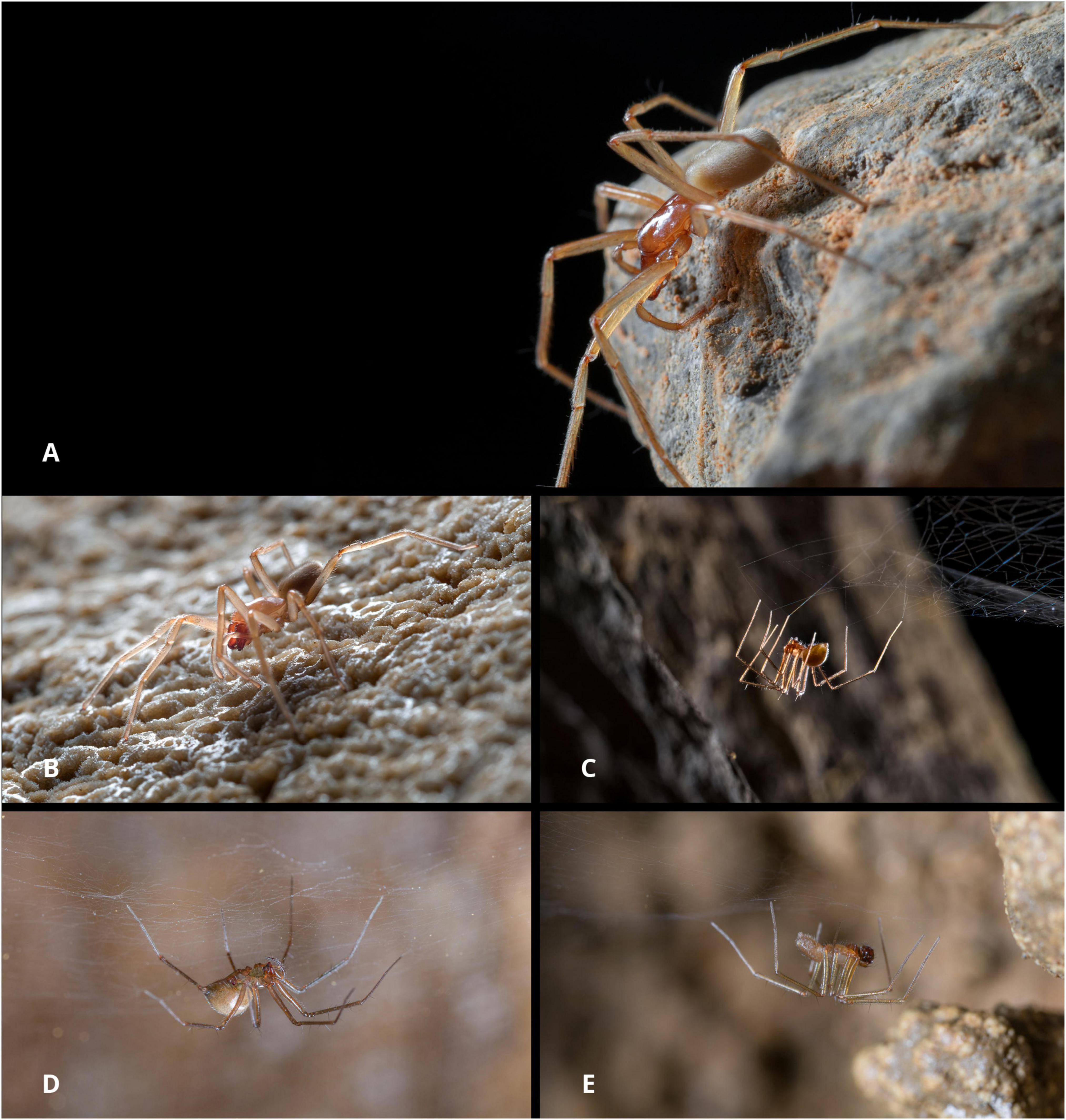
Figure 1. Photographs of the five studied species. (A) Parastalita stygia, (B) Stalita pretneri, (C) Troglohyphantes croaticus, (D) Troglohyphantes excavatus, (E) Troglohyphantes kordunlikanus. Photos by: (A,B) Tin Rožman; (C) Jana Bedek; (D,E) MP.

FIGURE 2

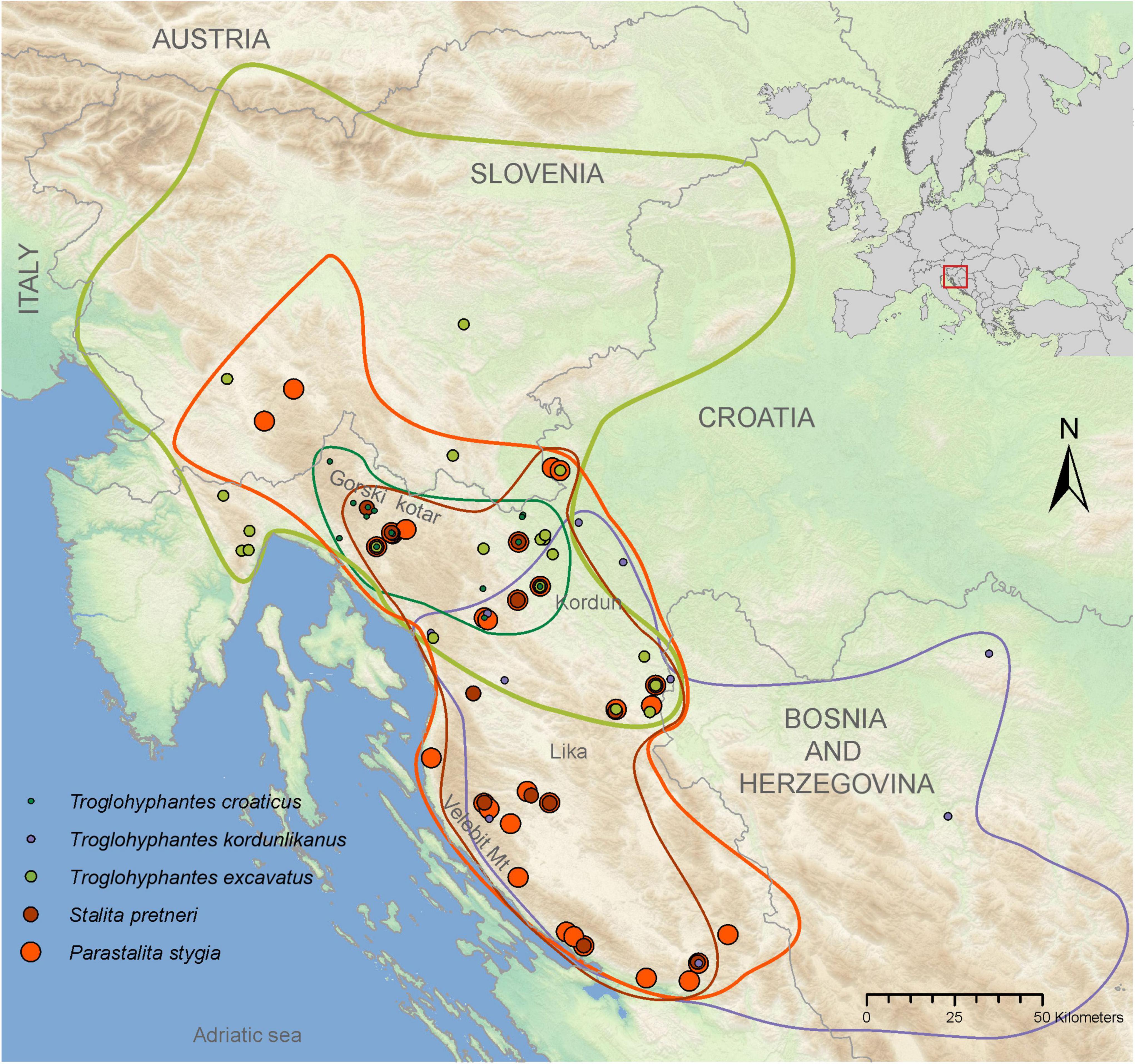
Figure 2. Map showing the distributions of each of the five studied species. Dots represent the localities from specimens used in this study, and lines in matching colors encircle the species’ distributions. Overlapping dots represent caves with more than one species. Changes in dot sizes are used as a means of showing overlapping species presences.

Cave fauna are generally difficult to sample due to the technical obstacles in entering and exploring the caves and pits (Zagmajster et al., 2010). In addition, population densities seem to be low and show a strong temporal variability of their presence. To overcome these sampling limitations, we took advantage of the sampling carried out over the past decades, stored in natural history collections. Despite not having been preserved in DNA-compliant conditions, these samples have the advantage of being accessible. Recent developments in molecular biology, such as hybridization capture methods, e.g., HyRAD (Suchan et al., 2016), facilitates recovery of genetic information from museum samples for which the DNA is often degraded and in low quantities (Toussaint et al., 2021). By applying museomics techniques, we retrieved DNA polymorphisms and inferred population genetic structures in each of the five species described above. Specifically, we applied the HyRAD technique and the popHyRAD pipeline (Gauthier et al., 2020) to specimens from the natural history collection of the Croatian Biospeleological Society (CBSS) from Zagreb, which holds one of the largest collections of cave spiders in the world. We then performed a comparative phylogeographic approach involving the five above mentioned co-distributed cave-dwelling spider species to test (1) if the degree of troglomorphism relates to the patterns of isolation by distance, and (2) whether the studied species underwent similar phylogeographic processes and thus share the same breaks in the spatial patterning of their genetic variation, or, alternatively, if spatial population structure is distinctive to each species.

Materials and methods

Sampling

Our sampling performed at the Croatian Biospeleological Society (CBSS Collection, Zagreb, Croatia), ZCSL (Zoological collection of SubBioLab, University of Ljubljana, Ljubljana, Slovenia), and ROC (Roman Ozimec collection, Zagreb, Croatia) natural history collections encompasses 117 specimens from the five studied species (i.e., 34 specimens of P. stygia, 26 of S. pretneri, 12 of T. kordunlikanus, 24 of T. excavatus, and 21 of T. croaticus) (Figure 2 and Supplementary Table 1A). The oldest sample was collected in 1974, 5 samples were collected before 2000, 49 samples were collected between 2000 and 2010, and 61 were collected between 2010 and 2018. Their preservation conditions varied in different concentrations of ethanol, ranging from absolute to 40% ethanol, and all samples were kept at room temperature (Supplementary Table 1).

Since the information on the level of troglomorphy as suggested by eye reduction and depigmentation for the three Troglohyphantes species was only reported in a few relatively old papers (Fage, 1919; Deeleman-Reinhold, 1978), and include very limited geographic sampling, we checked the level of depigmentation and eye reduction in all available specimens from the CBSS collection. Observed troglomorphic patterns are reported in Supplementary Table 1B. We used the QGIS software in order to represent the distribution of specimens on maps.

DNA extraction and HyRAD protocol

To retrieve DNA from old and poorly preserved samples, the HyRAD protocol (Suchan et al., 2016) was applied following Toussaint et al. (2021) with some modifications specified below. To produce the probes used in the capture process, we first extracted DNA from four fresh specimens corresponding to the studied species: sample psty_5115_1 for P. stygia, sample spre_5118 for S. pretneri, sample tcro_4274 for T. croaticus and T. excavatus (as the two species are closely related), and sample tkor_5227_1 for T. kordunlikanus (Supplementary Table 1A). Genomic DNA was extracted using Speedtools Tissue DNA Extraction Kit (Biotools), DNeasy Blood, and Tissue Kit (Qiagen) and QIAamp DNA Micro Kit (Qiagen), depending on the sample condition. The preparation of the ddRAD library comprised a digestion with the restriction enzymes MseI and PstI-HF (New England Biolabs, Ipswich, MA, USA), ligation of adaptors and individual barcodes, size selection with Blue Pippin (2% dye-free Agarose Gel Cassette marker V1, Sage Science) with a range of 190–240 bp and a final amplification by PCR for 20 cycles using NEBNext Hi-Fi 2X PCR Master Mix (New England Biolabs, Ipswich, MA, USA). An aliquot of the final library was sequenced on one lane of an Illumina MiSeq 150 bp paired-end at the Lausanne Genomic Technology Facility (LGTF) in order to obtain a sequence catalog of the loci represented in the ddRAD probes, and the rest of the library was transcribed into RNA probes and biotinylated using HiScribe T7 High Yield RNA Synthesis Kit (New England Biolabs, Ipswich, MA, USA).

Historical DNA from collection samples was extracted using the same DNA extraction kits as for the probes design, and in some cases only one or few legs were used through non-destructive extraction consisting in putting the material in a buffer with proteinase K overnight, and returning it back to the collection specimen. The purified DNA was quantified and the quality was assessed using a Fragment Analyzer. For specimens with large DNA fragment sizes (>1 kb) a shearing step was performed using the NEBNext^® dsDNA Fragmentase^® (New England Biolabs, Ipswich, MA, USA) protocol, except that only 1 μl of enzyme was used. A shotgun library preparation was applied to each sample following Suchan et al. (2016), comprising phosphorylation with T4 Polynucleotide Kinase, heat-denaturation, G-tailing with Terminal Transferase, second strand DNA synthesis with Klenow Fragment (3’–>5’ exo-) using a poly-C oligonucleotide, blunt-end reaction with T4 DNA Polymerase, barcoded adapters ligation to the phosphorylated end with T4 DNA ligase, and PCR amplification using Phusion U Hot Start DNA Polymerase (Thermo Scientific). Libraries were purified and quantified using Quant-iT PicoGreen^® dsDNA reagent (Invitrogen) on a Hidex Sense Microplate reader and pooled equimolarly based on their concentration. Hybridization capture was performed with a two-step capture at two temperatures, i.e., 55 and 65^°C to improve the stringency of the reaction, as suggested by Li et al. (2013) as well as Suchan et al. (2022). Enriched libraries were sequenced on two lanes of an Illumina HiSeq2500 using a paired-end 100 bp protocol at the LGTF.

Demultiplexing and Single Nucleotide Polymorphisms identification

The first part of the bioinformatic pipeline consisted in the identification of the ddRAD loci present in the probes specimens used for the capture, in order to build a reference catalog. The probe reads generated from the ddRAD libraries were demultiplexed according to barcodes and cleaned using Cutadapt v1.18 (Martin, 2011) to remove adaptors, bases with a quality lower than 20 and reads smaller than 30 bp. Read quality was checked using FastQC v0.11.8 (Babraham Institute, Babraham, England). Loci construction was performed for each species individually, except for the pair of sister species T. croaticus and T. excavatus. Ipyrad v0.7.30 (Eaton and Overcast, 2020) was used with a minimum depth of six and a clustering threshold of 0.80 (selected threshold after testing values of 0.70, 0.80, and 0.90). Shared loci were retained to build the reference catalogs for each species. In practice, a catalog of 23,031 loci was used for the mapping of T. croaticus and T. excavatus, a catalog of 20,691 loci for T. kordunlikanus, a catalog of 22,150 loci for P. stygia, and a catalog of 23,022 loci for S. pretneri. Reads from historical samples were cleaned using Cutadapt v1.18 (Martin, 2011) to remove barcodes, adaptors, terminal poly-Cs, and bases with a quality lower than 20 and reads smaller than 30 bp. Read quality was checked using FastQC v0.11.8 (Babraham Institute, Babraham, England). Clean reads were individually mapped on the corresponding probe catalogs using BWA-ALN v0.6 (Li and Durbin, 2009). Indels were realigned using the GATK IndelRealigner v3.8 (McKenna et al., 2010), PCR duplicates were removed using MarkDuplicates from the Picard toolkit v2.20.2¹, and base quality was rescaled using MapDamage v2.0 (Jónsson et al., 2013) to take into account post-mortem DNA deamination.

To verify the species status of each sample, the phyloHyRAD pipeline (Toussaint et al., 2021) was applied to reconstruct the ddRAD sequence alignment for each locus and perform phylogenetic inferences within the two groups. Consensus sequences were generated from the previous mapping files using samtools mpileup v1.4, bcftools v1.4 and vcfutils, keeping the main bases and a minimum coverage of three. Resulting consensus loci were combined from the shared loci resulting from the abovementioned iPyRAD analysis, i.e., at the family level for Dysderidae and at the genus level for Troglohyphantes. They were further aligned using MAFFT v7.407 (Katoh et al., 2002). Alignments were cleaned to keep loci shared by at least one third of the samples and checked manually. We finally obtained 1,915 loci for P. stygia, 989 loci for S. pretneri and 2,276 loci for the three Troglohyphantes species. Loci were concatenated using AMAS v1.02 (Borowiec, 2016). Best partitioning schemes were estimated using PartitionFinder2 (Lanfear et al., 2017), and corresponding models of nucleotide substitution were determined using ModelFinder (Kalyaanamoorthy et al., 2017). Phylogenetic inferences were performed on the concatenated alignment using IQ-TREE v 1.6.11 (Minh et al., 2020), and branch support was estimated using 1,000 ultrafast bootstraps along with 1,000 SH-aLRT tests.

To identify genetic variations in each species confirmed by the phylogenetic approach, the PopHyRAD pipeline was applied (Gauthier et al., 2020). A variant calling was performed between each sample from the same species using Freebayes v1.3.1 (Garrison and Marth, 2012). Single Nucleotide Polymorphisms (SNPs) were filtered to keep only bi-allelic SNPs with a calling quality above 100 and shared by at least 60% of the samples in each species using vcftools (Danecek et al., 2011). Finally, samples with more than 90% of missing data, i.e., 11 samples in total, were removed.

Population genetic structure analyses

In order to investigate population genetic structure in the five species, we extracted a subset of unlinked SNPs by randomly selecting one SNP per locus. To infer intraspecific genetic structures, we used principal component analysis (PCA) as implemented in the adegenet R package v2.1.5 (Jombart and Ahmed, 2011). PCA plots were performed using direct PCA values (Figure 3), and integrating eigenvalues to take into account the weight of the PC axis (Supplementary Figure 1). Secondly, a Bayesian admixture analysis as implemented in STRUCTURE v 2.3.4 (Pritchard et al., 2000) was performed. We ran analyses with K ranging from 1 to 10, assuming correlated allele frequencies and admixture, and performed 10 independent replicates for each K with 200,000 Markov chain Monte Carlo including a burn-in step of 10,000 iterations. We evaluated the number of genetic clusters that best describes our data according to log likelihoods of the data (LnPr (X| K) for each value of K (Pritchard et al., 2000) and the ΔK method (Evanno et al., 2005) with Structure Harvester (Earl and VonHoldt, 2012). We used CLUMPP and the Greedy algorithm to align multiple runs of STRUCTURE for the same K value (Jakobsson and Rosenberg, 2007), and distruct (Rosenberg, 2003) to plot the individual’s cluster membership probabilities. Additionally, to overcome the STRUCTURE constraints related to discrete population inference and to investigate putative continuous patterns of population structure, we also analyzed data under a model-based method that simultaneously infers continuous and discrete patterns integrating geographic distances, as implemented in conStruct (Bradburd et al., 2018). To test the best fit to the data between discrete versus continuous clusters, we used the cross-validation procedure implemented in the conStruct package for each species with K ranging from 1 to 10, with three repetitions for each K value, 15,000 iterations per repetition, and a training proportion of 0.9. The best K was identified based on comparing predictive accuracy for each K and for each model, i.e., with and without geographic distances. Considering that the larger the number of K tested, the larger the number of parameters implemented (potentially inducing an overparameterization and artificially increase the accuracy; Bradburd et al., 2018), the best K can be considered as the lowest K for which the accuracy has reached a plateau. Results were visualized using plots generated by conStruct.

FIGURE 3

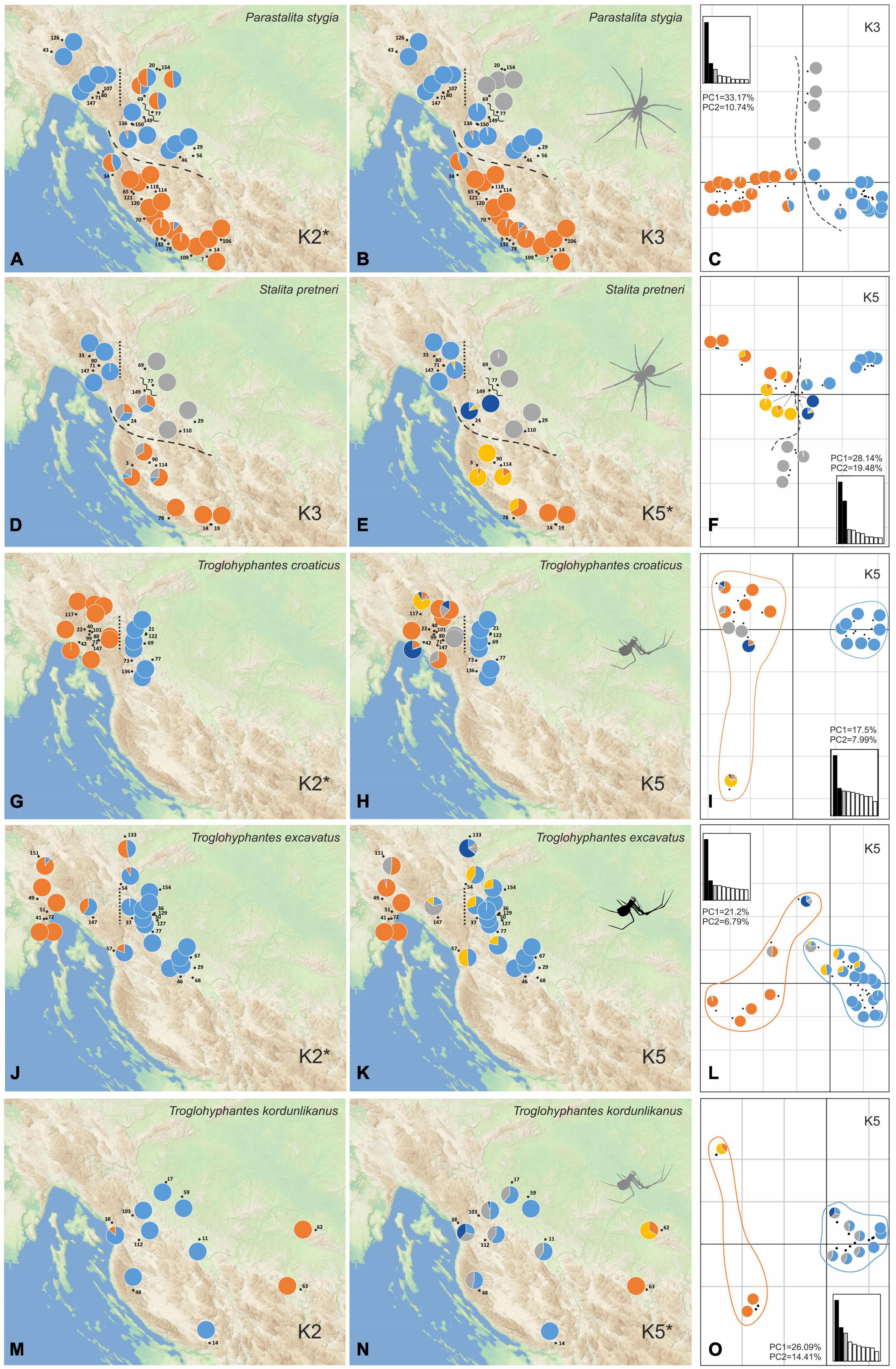
Figure 3. Population structure of the five studied species as inferred by STRUCTURE and principal component analyses (PCA) analyses. Colors on the pie charts correspond to the proportion of each specimen assigned to each of the genetic clusters inferred for a given K value. For each species, both the optimal K value and an additional one showing a relevant geographical pattern with good statistical support, according to log probabilities of the data (LnPr (X| K)), are presented. (A) Scatterplot of the first two PCA components is given for every species with a pie chart taken from one of the best K values associated with each locality. Main population breaks are marked with dashed and dotted lines. Parastalita stygia maps with K2 (A), K3 (B), and PCA (C); Stalita pretneri maps with K3 (D), K5 (E) and PCA (F); Troglohyphantes croaticus maps with K2 (G), K5 (H) and PCA (I); Troglohyphantes excavatus maps with K2 (J), K5 (K), and PCA (L); Troglohyphantes kordunlikanus maps with K2 (M), K5 (N), and PCA (O). In Troglohyphantes species PCAs (I,L,O), pies denote clustering with K5, and lines encircle K2 grouping. Optimal K for each species is marked with an asterisk.

For each population, descriptive statistics including the observed heterozygosities (Ho), mean gene diversities within population (Hs), allelic richness (Ar), and inbreeding coefficient (FIS) were estimated using the hierfstat package v0.5-7 (Goudet, 2005). Genetic differentiation (FST) between pairs of populations was estimated using vcftools (Danecek et al., 2011).

Isolation by distance (IBD) was calculated as follows: first, we performed a simple Mantel test as implemented in the R package vegan (Oksanen et al., 2020) to compare genetic and geographic distances for all sample pairs, and the significance was assessed with 999 permutations. Genetic distances were calculated as pairwise Nei’s distance values between samples using the dist.genpop function in the R package adegenet (Jombart and Ahmed, 2011), and geographic coordinates of caves were used to calculate straight-line geographic distances between sampling sites using the pointDist function in the R package enmSdm (Morelli et al., 2020). Secondly, a Spearman’s correlation test was applied for testing the correlation between genetic and geographic distances, and a linear model including an estimate of goodness-of-fit (R-squared), slope, and intercept, was set. These analyses were performed for each species. In addition, supplementary analyses were made for some species after excluding population pairs that demonstrated a pattern of very strong genetic isolation.

We used Stairway Plot 2 (Liu and Fu, 2020) to infer the demographic history of the two main genetic groups established by K = 2 in STRUCTURE for each species (Supplementary Table 2). Site frequency spectrums were estimated using easySFS.² We assumed a mutation rate per site per generation of 2.8 × 10^–9 as estimated for Drosophila melanogaster (Keightley et al., 2014), and a generation time of 2 years according to our knowledge on the species biology.

Results

Museomics and HyRAD efficiency

The HyRAD approach allowed the recovery of a large number of reads and loci from the historical samples regardless of their age and storage conditions (Supplementary Tables 1, 2). The capture and sequencing method resulted in a total of 470 million reads distributed across the 106 samples for which HyRAD was successfully applied (of a total of 117 samples) with a mean of 4.44 million reads per sample (sd = 1.63 millions). The cleaning of reads resulted in a loss of 2.3% of reads (details in Supplementary Table 2). The oldest sample in the analysis was a sample of T. croaticus (ARCBSS 3422) collected in 1974 and despite being nearly 50 years old, the analysis yielded 6.14 million reads. Mapping of historical clean reads to the corresponding probe catalog resulted in mean mapping percentage of 55.6% (sd 7.2). After another stringent cleaning step, this proportion decreased to 25.4% (sd 7.3), corresponding to a mean of 14,367 bi-allelic SNPs (sd 4657) shared by at least 60% of the samples in each species and a mean read coverage of 43.85 (Table 1 and Supplementary Table 2). Finally, in order to perform genetic structure analyses, we kept one single SNP per locus, resulting in a mean of 6847 unlinked SNP by sample (sd 1967). The summarized data on the number of samples, SNPs, and the overall percentage of missing data is given in Table 1 (see also Supplementary Table 2).

TABLE 1

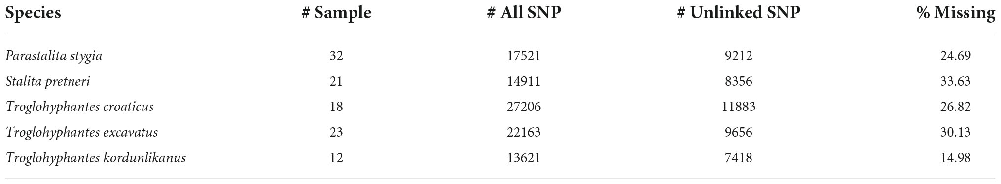
Table 1. Number of samples and single nucleotide polymorphisms (SNPs) per species after filtering steps.

Population genetic structure

Phylogenetic inferences performed on P. stygia, S. pretneri, and the three Troglohyphantes species, confirmed the morphological identifications made on the historical samples and their species-level status, at least on the basis of our sampling (Supplementary Figure 2). Population genetic analyses were then carried out within each species. The STRUCTURE and conStruct analyses showed different patterns of genetic clustering for each of the five studied species (STRUCTURE statistics and conStruc results are shown in Supplementary Table 3 and Supplementary Figure 3, respectively). For each species, a map was made with pie charts corresponding to the STRUCTURE Bayesian assignment probabilities per sampling location exemplified for the best run of each selected K values (Figure 3 and Supplementary Figures 3, 4). Supplementary Figures 3, 4 show the summed results of all K runs for each species. Overall, the conStruct results showed that the spatial model presents, for each species, a better accuracy than the non-spatial model (Supplementary Figure 3), highlighting the fact that the clustering recovered in the STRUCTURE analysis is not the consequence of isolation by distance alone. Thus, additional phylogeographic breaks or ecological traits potentially driving lineage divergence might be at work in the case of all five species studied here.

For P. stygia, STRUCTURE analyses yielded an optimal clustering value for K = 2 according to the ΔK criterion, while the log likelihood of the data [L (K) (mean ± SD)] (see Supplementary Table 3) increased steadily up to K = 6. ConStruct results also confirm the structuring of the samples in clear genetic groups; we observe a plateau in the accuracy values after K = 3, a result that might be interpreted as three clusters being the optimal way to partition the data, as well as a sustained contribution of these three groups to the total covariation between the clusters (Supplementary Figure 3A). The genetic clusters inferred by STRUCTURE at K = 2 follow a north-south geographical distribution pattern with the break being located in the northern Lika region (dashed line in Figures 3A–C). Several hybrid specimens were identified, one near the break-line, and a group of four samples in the central-north area. This main genetic differentiation is also denoted in the PCA analyses, with axis 1 describing the two main genetic groups (Figure 3C). The second best STRUCTURE clustering scenario according to the ΔK criterion is K = 3, which is also considered as the best K value in conStruct. It revealed the presence of a third cluster, distributed across the central and northern sampling area (gray in Figures 3B,C) and separated by two break lines from the central (blue) group—one in the eastern part of Gorski kotar region (dotted line in Figures 3A,B), and a second in the area of the Ogulin-Plaški valley (wavy line in Figures 3A,B). On the PCA, this separation is supported by axis two (Figure 3C). Analyses with a higher number of clusters, e.g., K = 6, revealed additional structuring within the large southern group, south to the northern Lika break (Supplementary Figure 4A).

For S. pretneri, STRUCTURE analyses showed that log probabilities of the data [L (K) (mean ± SD)] reached a plateau at K = 5. Also, the ΔK criterion indicated K = 5 as the best clustering solution, and K = 3 as the second best (Supplementary Table 3). In the conStruct analysis, accuracy reached a plateau after K = 5, similarly as revealed by STRUCTURE results, but additional spatial layers beyond K = 4 only contributed marginally to the total covariance among clusters. The same breaks as in P. stygia were recognized in S. pretneri−one in the northern Lika (dashed line in Figures 3D–F), one in the eastern part of the Gorski kotar region (dotted line in Figures 3D,E), and one in Ogulin-Plaški valley (wavy line in Figures 3D,E). The PCA yielded analogous results to those obtained with STRUCTURE, separating northern from southern populations along axis 1, and grouping populations according to their geographical location.

For T. croaticus the optimal clustering solution identified with STRUCTURE was K = 2 based on both the ΔK criterion and the log probabilities of the data (Supplementary Table 3)—there is a clear genetic and geographic separation between eastern (blue in Figure 3G) and western (orange in Figure 3G) individuals, and no hybrids were detected. In the conStruct results, the predictive accuracy reached a plateau at K = 2, and the layer contribution is clearly more important for the two main clusters even when the number of K tested is larger (Supplementary Figure 3C). In addition, the conStruct analysis revealed some level of admixture between them. The position of a genetic break at the eastern part of the Gorski kotar region (dotted line in Figures 3G,H) is the same as in the two Dysderidae species (Figures 3A,B,D,E). Although less supported by the ΔK criterion, the K = 5 in STRUCTURE, revealed substructuring only in the western group, with the locality Sniježna jama (cave 117, yellow in Figure 3H) genetically distant (Figure 3I) from the other samples, even those that were geographically very close. The other localities of the western group were more admixed (Figure 3H).

For T. excavatus the best K value according to the ΔK criterion in STRUCTURE was also K = 2, with K = 5 being the second best (Supplementary Table 3). In conStruct, the layer contribution analysis showed that one of the clusters had a dominant contribution, and that after K = 2 the contribution of other clusters was very limited suggesting also an optimal clustering at K = 2. Overall, we observed a similar situation at K = 2 as in T. croaticus with a break at the eastern part of the Gorski kotar region (dotted line in Figures 3J,K), separating eastern and western genetic groups (blue and orange in Figure 3J, respectively), but in addition, this species demonstrated a hybrid zone in the middle of its geographic range. At K = 5 the STRUCTURE analysis showed that western- and eastern-most specimens were fully assigned to one of the two groups already found at K = 2, while the samples at the geographic boundary showed some levels of admixture (Figure 3K). The PCA plot showed the same pattern with a clear separation between the two main clusters according to axis 1, which is the axis carrying the main proportion of the genetic variation (Figure 3L).

For T. kordunlikanus the best K values according to the ΔK criterion in STRUCTURE were K = 2 and K = 5 (Supplementary Table 3). In conStruct, the analysis of the layer contribution and the distribution of the clusters confirmed the separation into two clusters: the eastern group (orange on Figure 3M) was restricted to north-west Bosnia and Herzegovina, and the western group (blue in Figure 3N) was distributed across the whole species range in Croatia. This split into two clusters is also clear from the PCA along axis 1 (Figure 3O). At K = 5, although the statistical support in STRUCTURE was strong (Supplementary Table 3), none of the analyses did present any clear spatial pattern—the eastern group remains separated, while the whole western group is composed of admixed individuals from several genetic clusters, without any clear barrier to gene flow.

Our comparative analysis has shown distinctive spatial genetic structuring patterns for each species. At the same time several similarities were revealed: one genetic break at the eastern part of Gorski kotar region is common to four species (both Dysderidae, and T. croaticus and T. excavatus), and two breaks are shared by the two Dysderidae species, one in northern Lika, and the other in the area of the Ogulin-Plaški valley. In contrast, T. kordunlikanus did not share any pattern in genetic structure with the other four species, partly since its distribution only overlaps that of the others across a small area. Troglohyphantes kordunlikanus aside, the observed breaks among species have been revealed whatever method used (including the two conStruct variants, with or without embedding a spatial model). These results confirm that the discrete distribution of genetic variation reported in all species is not merely due to isolation by distance processes coupled with non-continuous sampling.

Despite a clear genetic structuring revealed by the population structure analyses, the genetic differentiation (FST) observed among the main populations remained limited (<0.07). Analysis of the different genetic diversity statistics showed a variability across populations and species, e.g., the species T. kordunlikanus seems to demonstrate a higher genetic diversity than the other species, as well as a lower inbreeding coefficient (FIS) (Table 2). However, these results should be considered with caution because of the small number of samples encompassed in our study. The demographic inference analysis showed a similar pattern among species and populations, i.e., an increase in population size 100,000–200,000 years ago, and then a progressive reduction (Supplementary Figure 5).

TABLE 2

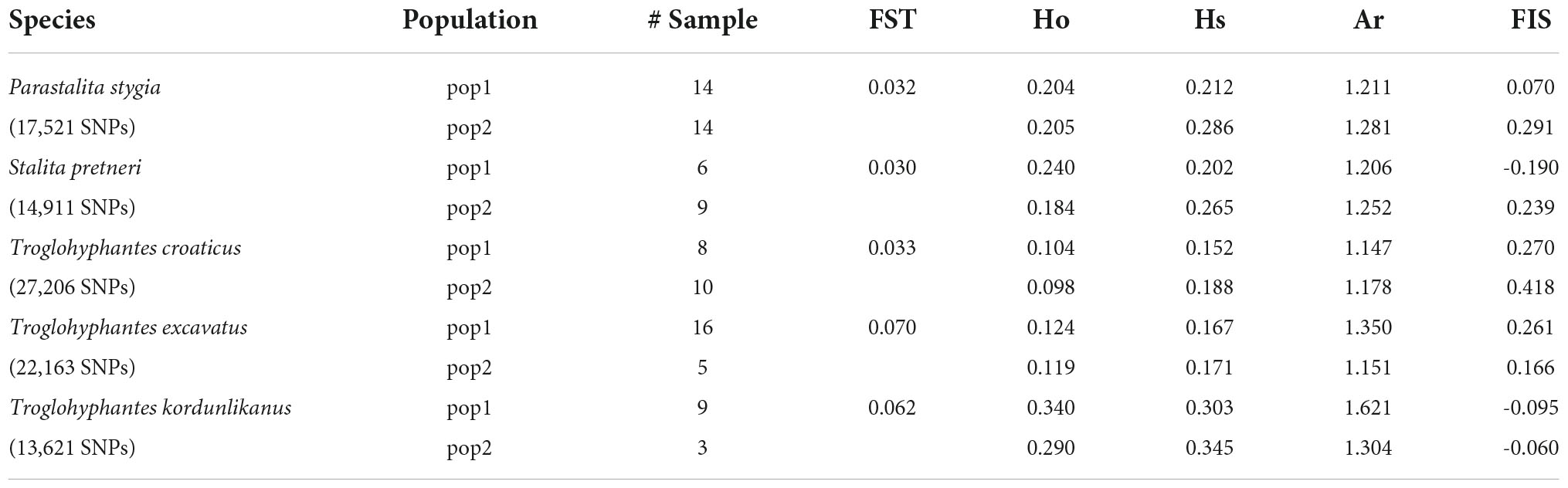
Table 2. Descriptive statistics estimated in each population identified by the best ΔK criterion, including the observed heterozygosities (Ho), mean gene diversities within population (Hs), allelic richness (Ar), inbreeding coefficient (FIS) and genetic differentiation (FST).

Isolation by distance

Significant isolation by distance was found in all five species (Table 3). Although Dysderidae species (S. pretneri and P. stygia) showed lower P-values than the three Troglohyphantes species as computed with a Mantel test, the slopes and intercepts were higher in the latter species (Table 3, Figure 4). Analyses conducted on the subset of populations not showing complete geographic and genetic isolation, mostly agreed with the whole-population analyses, with few exceptions (Supplementary Figure 6). In the case of the P. stygia central group (light blue on Figures 3A,B) the slope and the intercept were both lower than for the southern group (orange on Figures 3A,B). In T. croaticus the western group from the K = 2 analysis (orange on Figure 3G) showed a higher slope than the eastern group (blue on Figure 3G), while the western group found in T. kordunlikanus (blue on Figure 3M) showed no correlation between genetic and geographic distance (also visible from the structure analyses, Figure 3N). In the case of T. kordunlikanus, the sampling also included two easternmost populations (not hosting any of the other species)–interestingly, when these two populations were removed, isolation by distance was found to be non-significant.

TABLE 3

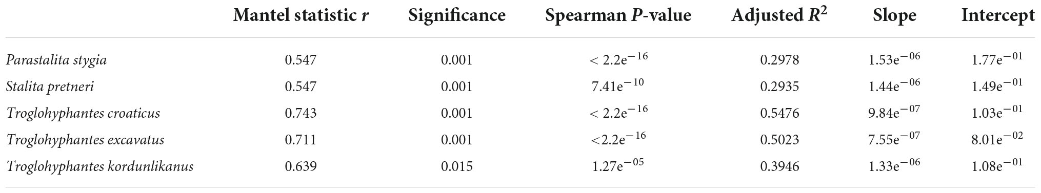
Table 3. Correlations among pairwise genetic and geographic distances based on Mantel tests and Spearman’s rho correlation coefficient. Adjusted R-squared (R²) of the linear model are included and linear equations are indicated in slope-intercept form.

FIGURE 4

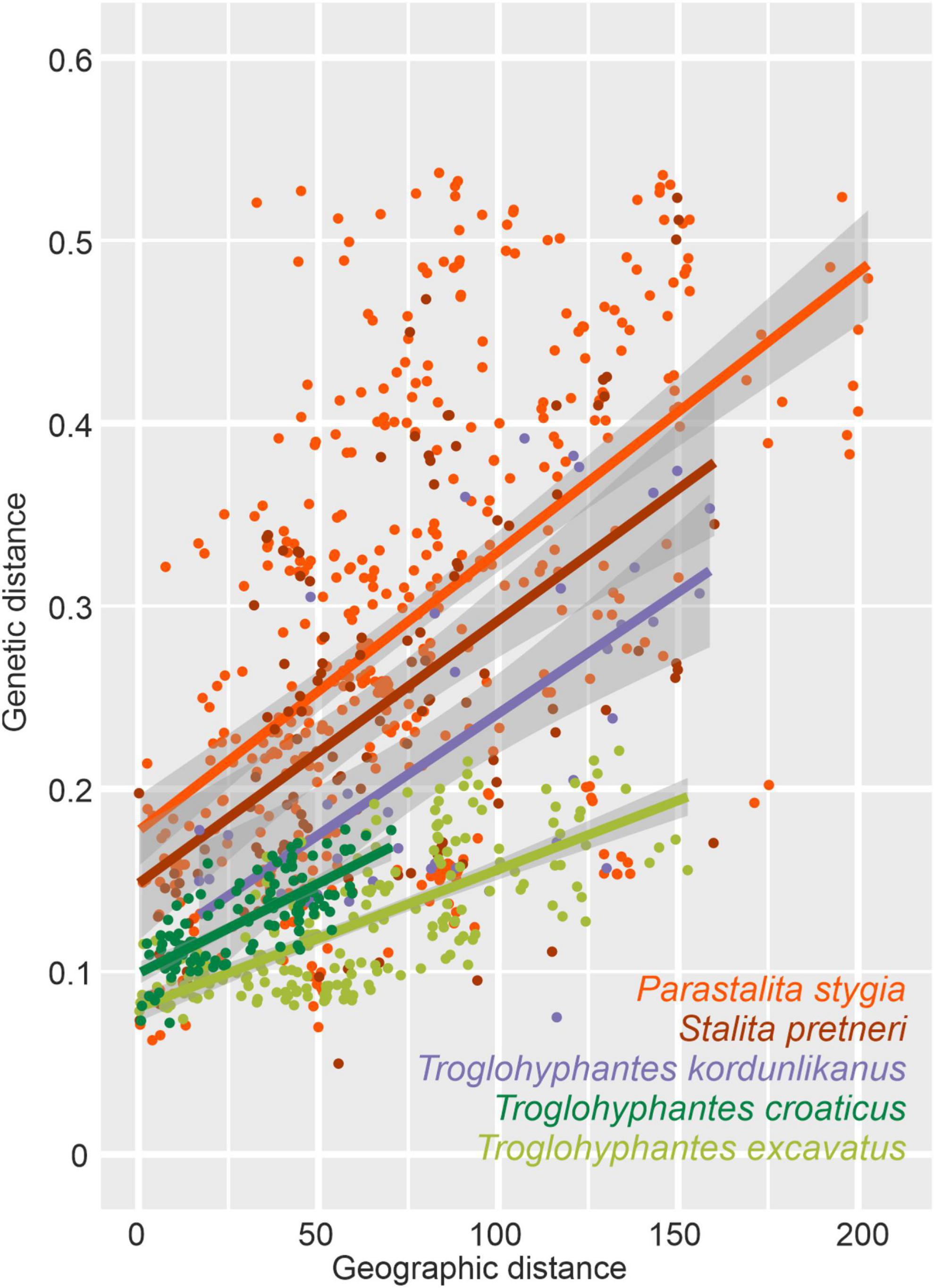
Figure 4. Plot showing the overall relationship between pairwise Nei’s genetic and linear geographical distances for each of the five studied species. A linear model is represented for each species, with corresponding information, adjusted R-squared (R²) and linear equations indicated in Table 3.

Troglomorphy

The Troglohyphantes species exhibited different levels of troglomorphic adaptation (Supplementary Table 1B). Troglohyphantes excavatus typically exhibited partial pigmentation and normal eyes, and only a few depigmented individuals were found. In the case of T. kordunlikanus, all specimens were depigmented, while their eyes were normally developed, and had thick or thin pigment rings around them. Interestingly, T. croaticus showed greater diversity, and a clear geographical segregation of troglomorphic traits. All individuals in the Kordun region (eastern part of the species’ distribution) were depigmented, most of them with eyes reduced to tiny white spots. Only a few individuals had normally developed eyes with thin black rings around them. In contrast, specimens from the western part (Gorski kotar region) were mostly depigmented, but with normally developed eyes with thin or thick black rings around them. Additionally, few individuals were strongly pigmented and with normally developed eyes, similar to what is found in T. excavatus.

Discussion

Museomics as a powerful tool to investigate “rare” species

Our study was made possible thanks to the application of museomics to historical samples. Indeed, as the availability of samples in the field is limited and our target organisms are difficult to sample in natura, the progressive accumulation of samples in the CBSS, ZCSL, and ROC natural history collections has made it possible to obtain enough samples to allow the comparative phylogeography inferences produced in this study. This opportunity to exploit tissues or even only DNA molecules from historical samples is associated with recent developments in museomics that allow the extraction and sequencing of degraded and low-concentration DNA from collection samples. Whereas it was previously only possible to recover specific gene sequences (usually short barcodes) through PCR-based approaches (Raxworthy and Smith, 2021), the development of innovative hybridization-capture methods such as HyRAD now allows the recovery of a large number of loci along the genome, and a more detailed investigation in a vast array of evolutionary questions (Suchan et al., 2016). The HyRAD method is based on the construction of probes from a ddRAD library followed by capture of these loci in the historical DNA. This approach allows capturing only the loci of interest and avoids inclusion of possible contaminants linked to historical samples.

Thus, in our study, we integrated 106 samples from the 117 samples initially sampled (91% success). At the scale of our study, the ability to capture DNA in a sample does not appear to be related to its age or to the concentration of DNA initially retrieved (Supplementary Table 2 and Supplementary Figure 7), as previously observed in a study on ground beetles using a similar method from the HyRAD family (Toussaint et al., 2021). Anecdotally, the oldest sample in the analysis collected in 1974 (tcro_3422) yielded enough information to be included in the analysis, which enabled us to detect a labeling mistake. The locality on the label was 200 km from the closest T. croaticus locality, but this sample grouped with a sample from the Vrelo cave (number 147) (Supplementary Figure 2), which is located in the middle of the species distribution. This, combined with the fact that the collector, the famous Dutch arachnologist Christa Deeleman-Reinhold, visited Vrelo cave just a few days after collecting sample tcro_3422, was sufficient evidence to demonstrate that the label was wrong and that the species distribution is not drastically different than previously known. Furthermore, thanks to the HyRAD approach, we were able to recover 9,212 loci (42% of the target loci), 8,356 loci (36% of the target loci), 11,883 loci (52% of the target loci), 9,656 loci (42% of the target loci), and 7,418 loci (35% of the target loci) for P. stygia, S. pretneri, T. croaticus, T. excavatus, and T. kordunlikanus, respectively. This is a larger amount of genetic information than what has been reported using UCEs, an alternative approach for retrieving molecular information from historical samples (Derkarabetian et al., 2019). The downside of the HyRAD strategy is that it requires the construction of a specific probe set for each group of closely related taxa, while UCE probes may enrich historical samples across a wider taxonomic range. As a matter of comparison, a recent UCE-based study, also on cave dwelling arachnids, recovered 289 loci (Derkarabetian et al., 2022). Meanwhile, HyRAD does not require any previous knowledge of genome sequences to produce orthologous data across samples. Moreover, HyRAD loci, which are derived from a ddRAD template, are potentially more informative at the intraspecific evolutionary scale, as exemplified by the present study. Whereas Derkarabetian et al. (2022) recovered a total of 1,277 SNPs from UCEs, we identified here a number of genetic polymorphisms larger by an order of magnitude, ranging between 13,621 and 27,206 SNPs, which enabled us to provide fine-scale insights into the population genetic structuring of our target species.

Geography, climate, and topography as possible causes for observed boundaries

In general, the distribution of genetic groups for all five species cannot be explained by current climate or habitat suitability that was modeled for the two Dysderidae species (Pavlek and Mammola, 2021; Supplementary Figure 8), and the reasons probably lie in the complex geological and climatic history, both of which are still not sufficiently explored for the area in question, and for the Dinarides in general.

Comparison of the spatial genetic structuring in the five species revealed common phylogeographic patterns except for T. kordunlikanus, whose different spatial distribution with only a narrow overlap with that of the four other species makes it difficult to identify common genetic breaks. A common barrier to gene flow has been observed for four of the five species (P. stygia, S. pretneri, T. croaticus, and T. excavatus) in the eastern part of the Gorski kotar region. One of the hypotheses to explain this barrier resides in differences in climatic conditions on both sides of the barrier. Indeed, the south-western side of this break shows a lower average temperature and higher precipitation levels than the other side (Supplementary Figure 8). For two species (S. pretneri and T. croaticus), no gene flow was identified across this barrier. Such strong genetic isolation between populations could explain morphological differences found on both sides of the genetic boundary for T. croaticus (see below). In the case of T. excavatus, a species able to use surface habitats for dispersal, some hybrid specimens were observed in this region, indicating the existence of detectable gene flow. Conversely, P. stygia seems to be able to disperse southwards across the break line, demonstrating good dispersal abilities also revealed by the large distribution observed for the central P. stygia lineage (blue pie charts in Figures 3A,B). Two other breaks are shared between the two Dysderidae species: one in the northern Lika region (dashed line in Figures 3A,B,D,E) that separates northern and southern clusters in both species, and a second one at the Ogulin-Plaški valley (wavy line in Figures 3A,B,D,E). While we were not able to identify the topographic features associated with the northern Lika break line, the second break could be explained by the specific geology of this area. The Ogulin-Plaški valley is a relatively narrow valley made from a less permeable rock (dolomites) than the surrounding area (Velić et al., 1980), resulting in surface streams that spring on one side, and sink on the other side of the valley. Our results might indicate that there is no underground system of crevices, which could be used for migration by the two Dysderidae species studied here, thus effectively isolating populations from the opposing sides of the valley. A similar explanation for the distribution throughout an area of dolomite deposits was invoked to explain the lower dispersal and deeper isolation of a lineage of the troglobiotic beetle Troglocharinus ferreri (Reitter, 1908) from Catalonia, when compared to another lineage distributed in a more permeable, and thus more connected limestone rock (Rizzo et al., 2017). The deep geographical structuring found in both Dysderidae species is comparable to that reported in North America cave beetles and harvesters for which geographic distance and landscape features each contributed to the formation of distinct genetic clusters (Kane and Brunner, 1986; Boyd et al., 2020; Derkarabetian et al., 2022). Conversely, no evidence of gene flow was detected among populations of troglobiotic spider and beetle species in caves less than 15 km apart (Balogh et al., 2020).

Links between genetic structure, isolation by distance, species biology, and ecology

Comparison of isolation by distance patterns shows that two factors, among others, could influence the genetic structuring of a given species, namely the level of troglomorphism and the foraging strategy (ground-dwellers vs. web-builders). Both Dysderidae species analyzed here are blind, depigmented, and restricted to cave habitats, while the three studied Troglohyphantes species display different levels of eye reduction, depigmentation, and the possibility, for two species at least, to disperse through surface habitats. The former observation would hint at a lower dispersal ability of Dysderidae and hence more structured populations. However, Troglohyphantes species build webs on which they spend most of their lives, while Dysderidae are active hunters which move swiftly around the cave in search for prey or mates, which, alternatively, would suggest better chances for dispersal through a well-connected underground system of crevices (Barr, 1967; Culver et al., 2004) for Dysderidae than for Troglohyphantes. In order to confront the two hypotheses, we examined IBDs in all five studied species and found that the slope and intercept of the correlation between geographic and genetic distances were always larger in Dysderidae than in Troglohyphantes. While the slopes and intercepts for one species of Troglohyphantes, i.e., T. kordunlikanus, are only marginally below those of the two species of Dysderidae, the pattern seems clearer still when the two easternmost populations of T. kordunlikanus (i.e., those that do not overlap with the other species’ distributions) are removed, as at this point no significant isolation by distance is retrieved. Altogether, our results suggest that lower levels of cave adaptation are associated with higher dispersal ability, regardless of the hunting strategy (Table 3 and Figure 4). Our study also reinforces the hypothesis that web-building species disperse better (T. kordunlikanus and T. excavatus even being found outside caves occasionally) and corroborate recent findings in sympatric cave springtails of the Salem Plateau in North America, which revealed stronger correlation between genetic and geographic distance in troglobionts when compared with troglophiles (Katz et al., 2018). Whereas differences in the intercept might reveal other scenarios such as different lineage age or timing of colonization in the studied clades (older species or older cave colonizers would demonstrate steeper slopes in the relationship between geographic and genetic distances), we currently lack data for alternative scenario testing. Different patterns were also unveiled among the Troglohyphantes species. Within the croaticus group, T. croaticus, which is the most troglomorphic species in the Troglohyphantes genus, and presumably the most dependent on its stable conditions—it was never collected outside caves—shows a steeper IBD than T. excavatus, indicating lower dispersal ability. Interestingly, genetic clusters in T. croaticus matched the morphological variation observed in the distribution of troglomorphic traits and in the levels of IBD, which warrants a re-examination of the species status across different populations. Indeed, the eastern group included mostly anophthalmic and depigmented individuals, while in the western group, which is genetically much more heterogeneous (Figures 3H,I and Supplementary Table 1B), a high degree of polymorphisms in troglomorphic traits was observed. This is also reflected in a higher IDB of the western group compared to the eastern one (Supplementary Figure 6). It is worth noting that no admixture was found between these two lineages. Contrastingly, T. excavatus showed a shallower IBD slope (Figure 4), suggesting higher connectivity among populations, which fits well with the fact that this species shows the lowest levels of troglomorphism among the five studied here. As mentioned above, results obtained for T. kordunlikanus are difficult to compare with those of the other species given the fact that its distribution only partly overlaps with that of the two other Troglohyphantes species as well as with the two Dysderidae species.

The fact that both Dysderidae species showed more marked IBD patterns was coherent with their blind and depigmented habitus, and the fact that they were never found outside caves—features we hypothesized would cause isolation of distant populations. Interestingly, both Dysderidae species demonstrate very similar values of Mantel and Spearman statistics, and geographical patterning of genetic lineages. Their ecological niche is also very similar, their distribution almost completely overlaps, and they can often be found in sympatry (Pavlek and Mammola, 2021). The only obvious difference is in the cheliceral morphology—P. stygia has elongated chelicerae, a trait that has been associated with trophic specialization (oniscophagy, i.e., feeding on woodlice) in other Dysderidae species (e.g., genus Dysdera, Rezaè et al., 2008)—which could imply that a segregation in diet may underlie and promote co-existence of the two species in sympatry.

Contrasting life-history traits of the two spider families are, as we predicted, reflected in their spatial population structures. Highly adapted Parastalita stygia and Stalita pretneri species show higher values of slope and intercept in the isolation by distance regression, suggesting lower dispersal ability, despite of their non-stationary and active way of life in caves. In contrast, lower dependency on cave conditions, as indicated by lower levels of troglomorphy, seems to be associated with higher dispersal rates in Trologyphantes species, regardless of their more stationary lifestyle. Spatial distribution of genetic groups revealed some common underlying breaks in the spatial genetic structure, indicating that geographic and climatic features probably influence dispersal potential of whole communities. Lastly, the existence of distinct genetic groups in all five studied species and their distinctive geographical distribution, should be considered when making management and conservation decisions.

Data availability statement

Raw reads are available on the NCBI BioProject PRJNA827597. The whole pipeline including custom scripts are available in the Github repository https://github.com/JeremyLGauthier/PHyRAD.

Author contributions

MP, NA, and MA designed the study. MP performed the sampling. MP and JB performed the lab work. JG and MP analyzed the molecular data, with contributions from VT. All authors took part in discussions concerning the analyses and result interpretations. MP, JG, and NA wrote the manuscript, with contributions from all authors.

Funding

This work was financially supported by a Marie Skłodowska-Curie Individual Fellowship (Grant agreement: 749867) (MP). Additional funding was provided by the Spanish Ministry of Economy and Competitiveness Grant CGL CGL2016-80651-P and the Agency for Management of University and Research Grants of Catalonia (2017SGR83) (both to MA). Open access funding was provided by the University of Geneva.

Acknowledgments

We sincerely thank all members of the Croatian Biospeleological Society, to Slavko Polak, Roman Ozimec, and all other speleologists and colleagues who collected the spider material. We also thank to SubBioLab from the University of Ljubljana for giving access to their collection. Thanks to Alba Enguídanos for her help with DNA isolation, to Tin Rožman for help with adjusting photographs, and also to Mladen Kuhta for help in interpreting the geological setup of the Ogulin-Plaški valley. The analyses were done on the Hercules server at the University of Barcelona and the Pyrgus server hosted by the City of Geneva.

Conflict of interest

The authors declare that the research was conducted in the absence of any commercial or financial relationships that could be construed as a potential conflict of interest.

Publisher’s note

All claims expressed in this article are solely those of the authors and do not necessarily represent those of their affiliated organizations, or those of the publisher, the editors and the reviewers. Any product that may be evaluated in this article, or claim that may be made by its manufacturer, is not guaranteed or endorsed by the publisher.

Supplementary material

The Supplementary Material for this article can be found online at: https://www.frontiersin.org/articles/10.3389/fevo.2022.910084/full#supplementary-material

Supplementary Figure 1 | For each species, principal component analysis (PCA) plots integrating eigenvalues.

Supplementary Figure 2 | Phylogenetic trees for (A) Parastalita stygia and Stalita pretneri, (B) Troglohyphantes croaticus, Troglohyphantes excavatus, and Troglohyphantes kordunlikanus. Branch support, SH-aLRT support/ultrafast bootstrap support (%), is shown for all branches.

Supplementary Figure 3 | Population structure of the five studied species as inferred by conStruct. For each species cross-validation results, layer contribution for each K value examined and admixture proportions pie charts are shown for spatial and non-spatial models. The colors in the bars show the contribution of each cluster or layer to the total covariance for each K. Each pie represents an individual. The color of the pie shows the proportion of the individual’s genome that is assigned to each of the K layers.

Supplementary Figure 4 | For each species, spatial genetic structuring for several K values (different for each species, based on STRUCTURE statistics) with pie charts corresponding to the Bayesian assignment probabilities per sampling locality exemplified for the best run of each K value. Summed results of all runs for each K value and for each species are shown as bar plots next to a map with the corresponding best K value or below the maps for the rest of K values. (A) Parastalita stygia, (B) Stalita pretneri, (C) Troglohyphantes croaticus, (D) Troglohyphantes excavatus, (E) Troglohyphantes kordunlikanus.

Supplementary Figure 5 | Stairway plots for each population, with population one in blue and population two in orange, in each species.

Supplementary Figure 6 | (A–C) Plots showing the relationship between genetic and simple geographical distance (expressed in km). (A) Parastalita stygia, plot for all samples together (black line), samples from central and southern group as in the K = 3 clustering analyzed together (green line), samples from southern (orange), and central (blue) group as in the K = 3 clustering. (B) Troglohyphantes croaticus, plot for all samples together (black line), samples from western (orange) and eastern (blue) groups as in the K = 2 clustering. (C) Troglohyphantes kordunlikanus, plot for all samples together (black line), and samples from western (blue) group as in the K = 2 clustering. (D) Correlations among pairwise genetic and geographic distances for groups within P. stygia, T. croaticus, and T. kordunlikanus based on Mantel tests and Spearman’s rho correlation coefficient.

Supplementary Figure 7 | Plots representing the relationship between the age of the specimens and the amount of reads and loci recovered (the samples included in the study are in black and the samples excluded in gray).

Supplementary Figure 8 | Distribution of each of the five species as a function of climatic factors. (A–C) Parastalita stygia; (D–F) Stalita preneri; (G,J) Troglohyphantes croaticus, (H,K) Troglohyphantes excavatus, (I,L) Troglohyphantes kordunlikanus. (A) Records of P. stygia overlapped with modeled habitat suitability taken from Pavlek and Mammola (2021) (white patches presenting areas of high suitability). (D) Records of S. pretneri overlapped with modeled habitat suitability taken from Pavlek and Mammola (2021) (white patches presenting areas of high suitability). (B,E,G–I) Species records overlapped with annual temperature values. (C,F,J–L) Species records overlapped with annual precipitation values. Climatic variables (annual precipitation and temperature) were taken from the WorldClim website (Fick and Hijmans (2017). Worldclim 2: New 1 km spatial resolution climate surfaces for global land areas. International Journal of Climatology, 37 (12), 4302–4315.).

Supplementary Table 1 | (A) Samples information. (B) Troglomorphism measurements.

Supplementary Table 2 | Sequencing statistics for each sample: raw reads number, clean reads number, raw number of mapped reads, % of mapped reads, number of mapped reads after cleaning, number of loci, and number of SNPs.

Supplementary Table 3 | Structure statistics for all five species. (A) Parastalita stygia, (B) Stalita pretneri, (C) Troglohyphantes croaticus, (D) Troglohyphantes excavatus, (E) Troglohyphantes kordunlikanus.

Footnotes

1. ^ http://broadinstitute.github.io/picard
2. ^ https://github.com/isaacovercast/easySFS

References

Balogh, A., Ngo, L., Zigler, K. S., and Dixon, G. (2020). Population genomics in two cave-obligate invertebrates confirms extremely limited dispersal between caves. Sci. Rep. 10:17554. doi: 10.1038/s41598-020-74508-9

PubMed Abstract | CrossRef Full Text | Google Scholar

Barr, T. C. (1967). Observations on the ecology of caves. Am. Nat. 101, 475–491.

Google Scholar

Barr, T. C. (1968). Cave ecology and the evolution of troglobites. Evol. Biol. 2, 35–102.

Google Scholar

Barr, T. C., and Holsinger, J. R. (1985). Speciation in cave faunas. Annu. Rev. Ecol. Syst. 16, 313–337.

Google Scholar

Borowiec, M. L. (2016). AMAS: a fast tool for alignment manipulation and computing of summary statistics. PeerJ 4:e1660. doi: 10.7717/peerj.1660

PubMed Abstract | CrossRef Full Text | Google Scholar

Borregaard, M. K., Amorim, I. R., Borges, P. A. V., Cabral, J. S., Fernández-Palacios, J. M., Field, R., et al. (2017). Oceanic island biogeography through the lens of the general dynamic model: assessment and prospect. Biol. Rev. 92, 830–853. doi: 10.1111/brv.12256

PubMed Abstract | CrossRef Full Text | Google Scholar

Boyd, O. F., Philips, T. K., Johnson, J. R., and Nixon, J. J. (2020). Geographically structured genetic diversity in the cave beetle Darlingtonea kentuckensis Valentine, 1952 (Coleoptera, Carabidae, Trechini, Trechina). Subterr. Biol. 34, 1–23. doi: 10.3897/subtbiol.34.46348

CrossRef Full Text | Google Scholar

Bradburd, G. S., Coop, G. M., and Ralph, P. L. (2018). Inferring continuous and discrete population genetic structure across space. Genetics 210, 33–52. doi: 10.1534/genetics.118.301333

PubMed Abstract | CrossRef Full Text | Google Scholar

Bregović, P., and Zagmajster, M. (2016). Understanding hotspots within a global hotspot - identifying the drivers of regional species richness patterns in terrestrial subterranean habitats. Insect Conserv. Divers. 9, 268–281. doi: 10.1111/icad.12164

CrossRef Full Text | Google Scholar

Caccone, A. (1985). Gene flow in cave arthropods: a qualitative and quantitative approach. Evolution 39, 1223–1235. doi: 10.1111/j.1558-5646.1985.tb05688.x

PubMed Abstract | CrossRef Full Text | Google Scholar

Christiansen, K. (2012). “Morphological adaptations,” in Encyclopedia of Caves, eds W. B. White and D. C. Culver (Oxford: Elsevier Academic Press), 517–528.

Google Scholar

Culver, D. C., Christman, M. C., Šereg, I., Trontelj, P., and Sket, B. (2004). The location of terrestrial species-rich caves in a cave-rich area. Subterr. Biol. 2, 27–32.

Google Scholar

Culver, D. C., Deharveng, L., Bedos, A., Lewis, J. J., Madden, M., Reddell, J. R., et al. (2006). The mid-latitude biodiversity ridge in terrestrial cave fauna. Ecography 29, 120–128.

Google Scholar

Curl, R. L. (1986). Fractal dimensions and geometries of caves. Math. Geol. 18, 765–783. doi: 10.1007/BF00899743

CrossRef Full Text | Google Scholar

Danecek, P., Auton, A., Abecasis, G., Albers, C. A., Banks, E., DePristo, M. A., et al. (2011). The variant call format and VCFtools. Bioinformatics 27, 2156–2158. doi: 10.1093/bioinformatics/btr330

PubMed Abstract | CrossRef Full Text | Google Scholar

Deeleman-Reinhold, C. L. (1971). Beitrag zur Kenntnis höhlenbewohnender Dysderidae (Araneida) aus Jugoslawien. Razpr. Slov. Akad. Znan. Umet. 14, 95–120.

Google Scholar

Deeleman-Reinhold, C. L. (1978). Revision of the cave-dwelling and related spiders of the genus Troglohyphantes Joseph (Linyphiidae), with special reference to the Yugoslav species. Razpr. slov. Akad. Znan. Umet. 23, 1–220.

Google Scholar

Derkarabetian, S., Benavides, L. R., and Gonzalo, G. (2019). Sequence capture phylogenomics of historical ethanol-preserved museum specimens: unlocking the rest of the vault. Mol. Ecol. Res. 19, 1531–1544. doi: 10.1111/1755-0998.13072

PubMed Abstract | CrossRef Full Text | Google Scholar

Derkarabetian, S., Paquin, P., Reddell, J., and Hedin, M. (2022). Conservation genomics of federally endangered Texella harvester species (Arachnida, Opiliones, Phalangodidae) from cave and karst habitats of central Texas. Conserv. Genet. 23, 401–416. doi: 10.1007/s10592-022-01427-9

CrossRef Full Text | Google Scholar

Earl, D. A., and VonHoldt, B. M. (2012). Structure harvester: a website and program for visualizing structure output and implementing the Evanno method. Conserv. Genet. Resour. 4, 359–361. doi: 10.1007/s12686-011-9548-7

CrossRef Full Text | Google Scholar

Eaton, D. A. R., and Overcast, I. (2020). ipyrad: interactive assembly and analysis of RADseq datasets. Bioinformatics 36, 2592–2594. doi: 10.1093/bioinformatics/btz966

PubMed Abstract | CrossRef Full Text | Google Scholar

Eme, D., Malard, F., Konecny-Dupré, L., Lefébure, T., and Douady, C. J. (2013). Bayesian phylogeographic inferences reveal contrasting colonization dynamics among European groundwater isopods. Mol. Ecol. 22, 5685–5699. doi: 10.1111/mec.12520

PubMed Abstract | CrossRef Full Text | Google Scholar

Evanno, G., Regnaut, S., and Goudet, J. (2005). Detecting the number of clusters of individuals using the software structure: a simulation study. Mol. Ecol. 14, 2611–2620. doi: 10.1111/j.1365-294X.2005.02553.x

PubMed Abstract | CrossRef Full Text | Google Scholar

Fage, L. (1919). Etudes sur les araignées cavernicoles. III. Sur le genre Troglohyphantes. Biospelogica XL. Arch. Zool. Exp. Gén. 55, 55–148.

Google Scholar

Fick, S. E., and Hijmans, R. J. (2017). Worldclim 2: new 1-km spatial resolution climate surfaces for global land areas. Int. J. Climatol. 37, 4302–4315.

Google Scholar

Garrison, E., and Marth, G. (2012). Haplotype-based variant detection from short-read sequencing. arXiv [Preprint]. doi: 10.48550/arXiv.1207.3907

PubMed Abstract | CrossRef Full Text | Google Scholar

Gauthier, J., Pajkovic, M., Neuenschwander, S., Kaila, L., Schmid, S., Orlando, L., et al. (2020). Museomics identifies genetic erosion in two butterfly species across the 20th century in Finland. Mol. Ecol. Resour. 20, 1191–1205. doi: 10.1111/1755-0998.13167

PubMed Abstract | CrossRef Full Text | Google Scholar

Goudet, J. (2005). Hierfstat, a package for R to compute and test hierarchical F-statistics. Mol. Ecol. Notes 5, 184–186. doi: 10.1111/j.1471-8286.2004.00828.x

CrossRef Full Text | Google Scholar

Hedin, M. (1997). Molecular phylogenetics at the population/species interface in cave spiders of the southern Appalachians (Araneae: Nesticidae: Nesticus). Soc. Mol. Biol. Evol. 14, 309–324. doi: 10.1093/oxfordjournals.molbev.a025766

PubMed Abstract | CrossRef Full Text | Google Scholar

Howarth, F. G. (1987). Evolutionary ecology of aeolian and subterranean habitats in Hawaii. Tree 2, 220–223. doi: 10.1016/0169-5347(87)90025-5

PubMed Abstract | CrossRef Full Text | Google Scholar

Isaia, M., Mammola, S., Mazzuca, P., Arnedo, M. A., and Pantini, P. (2017). Advances in the systematics of the spider genus Troglohyphantes (Araneae, Linyphiidae). Syst. Biodivers. 15, 307–326. doi: 10.1080/14772000.2016.1254304

CrossRef Full Text | Google Scholar

Jakobsson, M., and Rosenberg, N. A. (2007). CLUMPP: a cluster matching and permutation program for dealing with label switching and multimodality in analysis of population structure. Bioinformatics 23, 1801–1806. doi: 10.1093/bioinformatics/btm233

PubMed Abstract | CrossRef Full Text | Google Scholar

Jalžić, B., Bedek, J., Bilandžija, H., Bregović, P., Cvitanović, H., Èuković, T., et al. (2013). The Cave Type Localities Atlas of Croatian Fauna, volume 2. Zagreb: CBSS.

Google Scholar

Jombart, T., and Ahmed, I. (2011). adegenet 1.3-1: new tools for the analysis of genome-wide SNP data. Bioinformatics 27, 3070–3071. doi: 10.1093/bioinformatics/btr521

PubMed Abstract | CrossRef Full Text | Google Scholar

Jónsson, H., Ginolhac, A., Schubert, M., Johnson, P. L. F., and Orlando, L. (2013). mapDamage2.0: fast approximate Bayesian estimates of ancient DNA damage parameters. Bioinformatics 29, 1682–1684. doi: 10.1093/bioinformatics/btt193

PubMed Abstract | CrossRef Full Text | Google Scholar

Kalyaanamoorthy, S., Minh, B. Q., Wong, T. K. F., Von Haeseler, A., and Jermiin, L. S. (2017). ModelFinder: fast model selection for accurate phylogenetic estimates. Nat. Methods 14, 587–589. doi: 10.1038/nmeth.4285

PubMed Abstract | CrossRef Full Text | Google Scholar

Kane, T. C., and Brunner, G. D. (1986). Geographic variation in the cave beetle Neaphaenops tellkampfi (Coleoptera: Carabidae). Psyche 93, 231–251. doi: 10.1155/1986/86164

CrossRef Full Text | Google Scholar

Katoh, K., Misawa, K., Kuma, K., and Miyata, T. (2002). MAFFT: a novel method for rapid multiple sequence alignment based on fast Fourier transform. Nucleic Acids Res. 30, 3059–3066. doi: 10.1093/nar/gkf436

PubMed Abstract | CrossRef Full Text | Google Scholar

Katz, A. D., Taylor, S. J., and Davis, M. A. (2018). At the confluence of vicariance and dispersal: phylogeography of cavernicolous springtails (Collembola: Arrhopalitidae, Tomoceridae) codistributed across a geologically complex karst landscape in Illinois and Missouri. Ecol. Evol. 8, 10306–10325. doi: 10.1002/ece3.4507

PubMed Abstract | CrossRef Full Text | Google Scholar

Keightley, D. P., Ness, R. W., Halligan, D. L., and Haddrill, P. R. (2014). Estimation of the spontaneous mutation rate per nucleotide site in a Drosophila melanogaster Full-Sib family. Genetics 196, 313–320. doi: 10.1534/genetics.113.158758

PubMed Abstract | CrossRef Full Text | Google Scholar

Lanfear, R., Frandsen, P. B., Wright, A. M., Senfeld, T., and Calcott, B. (2017). Partitionfinder 2: new methods for selecting partitioned models of evolution for molecular and morphological phylogenetic analyses. Mol. Biol. Evol. 34, 772–773. doi: 10.1093/molbev/msw260

PubMed Abstract | CrossRef Full Text | Google Scholar

Lefébure, T., Douady, C. J., Gouy, M., Trontelj, P., Briolay, J., and Gibert, J. (2006). Phylogeography of a subterranean amphipod reveals cryptic diversity and dynamic evolution in extreme environments. Mol. Ecol. 15, 1797–1806. doi: 10.1111/j.1365-294X.2006.02888.x

PubMed Abstract | CrossRef Full Text | Google Scholar

Li, C., Hofreiter, M., Straube, N., Corrigan, S., and Naylor, G. J. P. (2013). Capturing protein-coding genes across highly divergent species. Biotechniques 54, 321–326. doi: 10.2144/000114039

PubMed Abstract | CrossRef Full Text | Google Scholar

Li, H., and Durbin, R. (2009). Fast and accurate short read alignment with Burrows-Wheeler transform. Bioinformatics 25, 1754–1760. doi: 10.1093/bioinformatics/btp324

PubMed Abstract | CrossRef Full Text | Google Scholar

Liu, X., and Fu, Y.-X. (2020). Stairway Plot 2: demographic history inference with folded SNP frequency spectra. Genome Biol. 21:280. doi: 10.1186/s13059-020-02196-9

PubMed Abstract | CrossRef Full Text | Google Scholar

Mammola, S., and Isaia, M. (2017). Spiders in caves. Proc. R. Soc. B Biol. Sci. 284:20170193. doi: 10.1098/rspb.2017.0193

PubMed Abstract | CrossRef Full Text | Google Scholar

Martin, M. (2011). Cutadapt removes adapter sequences from high-throughput sequencing reads. EMBnet J. 17:10. doi: 10.14806/ej.17.1.200

CrossRef Full Text | Google Scholar

McKenna, A., Hanna, M., Banks, E., Sivachenko, A., Cibulskis, K., Kernytsky, A., et al. (2010). The genome analysis toolkit: a MapReduce framework for analyzing next-generation DNA sequencing data. Genome Res. 20, 1297–1303. doi: 10.1101/gr.107524.110

PubMed Abstract | CrossRef Full Text | Google Scholar

Mihevc, A., Prelošek, M., and Zupan Hajna, N. (2010). Introduction to the Dinaric Karst. Postojna: Karst Research Institute and Research Centre of the Slovenian Academy of Sciences and Arts.

Google Scholar

Minh, B. Q., Schmidt, H. A., Chernomor, O., Schrempf, D., Woodhams, M. D., von Haeseler, A., et al. (2020). IQ-TREE 2: new models and efficient methods for phylogenetic inference in the genomic era. Mol. Biol. Evol. 37, 1530–1534. doi: 10.1093/molbev/msaa015

PubMed Abstract | CrossRef Full Text | Google Scholar

Morelli, T. L., Smith, A. B., Mancini, A. N., Balko, E. A., Borgerson, C., Dolch, R., et al. (2020). The fate of Madagascar’s rainforest habitat. Nat. Clim. Change 10, 89–96. doi: 10.1038/s41558-019-0647-x

CrossRef Full Text | Google Scholar

Oksanen, J., Blanchet, F. G., Friendly, M., Kindt, R., Legendre, P., McGlinn, D., et al. (2020). vegan: Community Ecology Package. R Packag. version 2.5-6.

Google Scholar

Pavlek, M., and Mammola, S. (2021). Niche-based processes explaining the distributions of closely related subterranean spiders. J. Biogeogr. 48, 118–133. doi: 10.1111/jbi.13987

CrossRef Full Text | Google Scholar

Pritchard, J. K., Stephens, M., and Donnelly, P. (2000). Inference of population structure using multilocus genotype data. Genetics 155, 945–959. doi: 10.1093/genetics/155.2.945

PubMed Abstract | CrossRef Full Text | Google Scholar

Raxworthy, C. J., and Smith, B. T. (2021). Mining museums for historical DNA: advances and challenges in museomics. Trends Ecol. Evol. 36, 1049–1060. doi: 10.1016/j.tree.2021.07.009

PubMed Abstract | CrossRef Full Text | Google Scholar

Rezaè, M., Pekar, S., and Lubin, Y. (2008). How oniscophagous spiders overcome woodlouse armour. J. Zool. 275, 64–71.

Google Scholar

Ribera, I., Cieslak, A., Faille, A., and Fresneda, J. (2018). “Historical and ecological factors determining cave diversity,” in Cave Ecology, eds O. T. Moldovan, L. Kováè, and S. Halse (Berlin: Springer), 229–252. doi: 10.1007/978-3-319-98852-8_10

CrossRef Full Text | Google Scholar

Rizzo, V., Sánchez-Fernández, D., Alonso, R., Pastor, J., and Ribera, I. (2017). Substratum karstificability, dispersal and genetic structure in a strictly subterranean beetle. J. Biogeogr. 44, 2527–2538. doi: 10.1111/jbi.13074

CrossRef Full Text | Google Scholar

Rosenberg, N. A. (2003). distruct: a program for the graphical display of population structure. Mol. Ecol. Notes 4, 137–138. doi: 10.1046/j.1471-8286.2003.00566.x

CrossRef Full Text | Google Scholar

Salces-Castellano, A., Patiño, J., Alvarez, N., Andújar, C., Arribas, P., Braojos-Ruiz, J. J., et al. (2020). Climate drives community-wide divergence within species over a limited spatial scale: evidence from an oceanic island. Ecol. Lett. 23, 305–315. doi: 10.1111/ele.13433

PubMed Abstract | CrossRef Full Text | Google Scholar

Sbordoni, V., Allegrucci, G., and Cesaroni, D. (2000). Population genetic structure, speciation and evolutionary rates in cave-dwelling organisms. Subterr. Ecosyst. 24, 459–483. doi: 10.1093/jhered/esv078

PubMed Abstract | CrossRef Full Text | Google Scholar

Sket, B. (2012). “Diversity patterns in the Dinaric Karst,” in Encyclopedia of Caves, eds W. B. White and D. C. Culver (Oxford: Elsevier Academic Press), 228–238.

Google Scholar

Sket, B., Paragamian, K. K., and Trontelj, P. (2004). A census of the obligate subterranean fauna of the Balkan Peninsula. Balk. Biodivers. Pattern Process Eur. Hotspot 1540, 309–322. doi: 10.1007/978-1-4020-2854-0_18

CrossRef Full Text | Google Scholar

Suchan, T., Kusliy, M. A., Khan, N., Chauvey, L., Tonasso-Calvière, L., Schiavinato, S., et al. (2022). Performance and automation of ancient DNA capture with RNA hyRAD probes. Mol. Ecol. Resour. 22, 891–907. doi: 10.1111/1755-0998.13518

PubMed Abstract | CrossRef Full Text | Google Scholar

Suchan, T., Pitteloud, C., Gerasimova, N. S., Kostikova, A., Schmid, S., Arrigo, N., et al. (2016). Hybridization capture using RAD probes (hyRAD), a new tool for performing genomic analyses on collection specimens. PLoS One 11:e0151651. doi: 10.1371/journal.pone.0151651

PubMed Abstract | CrossRef Full Text | Google Scholar

Thaler, K. (1986). Über einige Funde von Troglohyphantes-Arten in Kärnten (Österreich) (Arachnida, Aranei: Linyphiidae). Carinthia II 176, 287–302.

Google Scholar

Toussaint, E. F. A., Gauthier, J., Bilat, J., Gillett, C. P. D. T., Gough, H. M., Lundkvist, H., et al. (2021). HyRAD-X exome capture museomics unravels giant ground beetle evolution. Genome Biol. Evol. 13, 1–18. doi: 10.1093/gbe/evab112

PubMed Abstract | CrossRef Full Text | Google Scholar

Trontelj, P. (2018). “Structure and genetics of cave populations,” in Cave Ecology, eds O. T. Moldovan, L. Kováè, and S. Halse (Berlin: Springer), 269–292.

Google Scholar

Velić, I., Sokaè, B., and Šćavnièar, B. (1980). Tumaè za list Ogulin. Osnovna Geološka Karta SFRJ 1:100.

Google Scholar

Zagmajster, M., Culver, D. C., Christman, M. C., and Sket, B. (2010). Evaluating the sampling bias in pattern of subterranean species richness: combining approaches. Biodivers. Conserv. 19, 3035–3048. doi: 10.1007/s10531-010-9873-2

CrossRef Full Text | Google Scholar

Zimmerman, E. C. (1949). Insects of Hawaii. Honolulu: University of Hawai‘i Press.

Google Scholar

Zupan Hajna, N. (2019). “Dinaric karst—Geography and geology,” in Encyclopedia of Caves, eds C. C. David and W. B. White (Cambridge, MA: Academic Press), 353–362.

Google Scholar