A dynamic framework for assessing and managing risks to ecosystems from fisheries: demonstration for conserving the krill-based food web in Antarctica

1. Introduction

Fisheries can impact ecosystems in many ways, including disruption of the dynamics of species targeted by the fishery or those killed incidentally in fishing operations, such as seabirds, destruction of habitat and the concomitant disruption of associated species, such as bottom fisheries impacts on reef systems, and alteration of food webs through the removal of species. The ecosystem approach to fisheries has been considered since “Our Common Future” (World Commission on Environment and Development, 1987) and the rise of sustainable development. The policy on what constitutes ecosystem-based fisheries management (EBFM) is articulated by the UN Food and Agriculture Organisation (FAO, 2003), following their publication of the precautionary approach to fisheries (FAO, 1996).

Emphases on EBFM have varied between a number of approaches. First, methods to implement ecosystem-oriented policies in decision rules and actions have been developed (Constable et al., 2000; Constable, 2006). Second, ecosystem risks of fishery management strategies are being evaluated using dynamic modelling, such as for understanding the food web effects of fishing (Constable, 2002, 2004, 2005; Fulton et al., 2019). Last, vulnerable species and habitats that may be directly affected are being identified and action taken to minimise impacts on them, such as for eliminating by-catch or avoiding sensitive areas (Smith et al., 2007; Constable, 2011).

All approaches aim to reduce risk of fisheries to whole, or components of, ecosystems. Unless of course, the management strategy is reactive, waiting for damage to be detected before action is taken; a strategy that obviously fails to meet ecosystem objectives because the damage has been done. Approaches aiming to keep risk of damage to a low level, risk assessments, sometimes called a precautionary approach, may seem to be costly, particularly when some argue that everything needs to be measured to properly assess risk. However, qualitative ranking of conditions to be avoided or reduced may be a first step in management before quantitative assessments of risk can be done (Smith et al., 2007). Consider the difference in approaches to minimising incidental seabird mortality in longline fisheries compared to reducing risk through stock assessments in the krill fishery by the Commission for the Conservation of Antarctic Marine Living Resources (CCAMLR) (Constable et al., 2000).

Stock assessments aim to provide sustainable catch limits for a region and for a designated time period, say one or 2 years. A particular challenge for managers is when fishing may become concentrated in space or time within the assessed region, causing ecosystem effects. Ecosystem risks may be related to areas fixed in space, such as reefs, or at particular times of the year, such as breeding periods, or some combination of the two, such as nursery areas. These risks may arise from fishing effort, such as the length of longline set or swept area of trawls, or simply from the total catch. The question then arises as to how to use ecosystem-oriented risk assessments to set finer-scale spatial and temporal measures to control a fishery in order to reduce the potential for ecosystem effects. Here, we present a dynamic framework of risk assessment and management that can help distribute a fishery in space and time to avoid ecosystem effects. It enables use of available data and knowledge to set ecosystem-based catch controls on a fishery to maintain ecosystem risk at a low level, and then be easily updated as new information and assessments arise.

While the framework could be applied to determining how fishery controls may be varied over years, we focus on developing the framework for its use to distribute a fishery in space and between the seasons within a year to maintain low risk of ecosystem impacts despite spatial variability in data and knowledge. The approach may be coupled with considerations of the conservation of biodiversity in marine protected areas (Grorud-Colvert et al., 2021) and can serve to address the potential overlap of fisheries with areas of high conservation value. It is designed to account for heterogeneity in ecosystems, including the different spatial and temporal scales at which organisms function. We develop the framework in the first section of the paper, including a simple illustration of its application. In the framework we include methods for using closed areas to offset risk or for conserving biodiversity of high conservation value. We also present methods that could be used to account for uncertainties in input data and knowledge. In the second section, we present a real-world illustration of the application of the framework to managing risks of food web effects of fishing for Antarctic krill in the Southern Ocean.

2. Framework for managing heterogeneity in risk

With perfect knowledge, catches can be distributed to avoid high risk of ecosystem impacts, equivalent to using an accurate dynamic ecosystem model for determining a spatially and temporally resolved fishing strategy. However, with imperfect knowledge, how might we avoid ecosystem impacts in a heterogeneous world?

2.1. Composite risk index

Risk, r, is the product of the probability, p, of the catch or effort from the fishery (F) and the probability of significant ecosystem impact, E, given the fishery (see Fenton and Neil, 2013 for a broad discussion on mathematical formulation of risk):

$\begin{array}{ll}r=p\left(F\right)p\left(E\mathrm{|}F\right)& (1)\end{array}$

Here, we are seeking specific fishery controls in space and time to reduce risk to acceptable levels, thereby setting p(F) to equal 1. If the relationship between F and probability of significant ecosystem impacts is known then we can easily solve for the limits to the fishery that satisfactorily reduces risk. This logic underpins the framework. Moreover, it can be usefully applied even when the relationship between the magnitude of fishing and impacts is only approximated in the early stages of a fishery.

2.1.1. Index of risk

The concept of significant ecosystem impact arising from F has three parts: (i) a combination of specific effects on the ecosystem, (ii) a judgement on the degree to which levels of effects are regarded as significant impacts, and (iii) the method for combining the effects into a single risk. In reality, Equation 1 becomes an index of risk, R, ranging from 0 to 1. The probabilities of the effects are standardised to a scale of significance of impact in order for them to be combined. This may be achieved by rescaling the effects to significance of impact and retaining the probabilities, or by rescaling the probabilities to range from 0 to 1 and retaining the levels of effects. The latter may be done in order to keep the discussion around observed effects/biological quantities rather than more abstract quantities. For this reason and because probabilities may be expert judgements in early stages of applying the framework, we use the term “pseudo-probabilities” for individual ecosystem effects in presenting the framework.

The index of risk for a given area will be derived from pseudo-probabilities, r(F)_n’, relating to n different risks. The combining of pseudo-probabilities cannot be additive. Nor can it result in the apparent risk indicated by the index to be less than any individual risk. We choose a formulation that increases the index as more risks arising from fishing activities are included:

$\begin{array}{ll}R\left(F\right)=1-\underset{n}{\Pi }(1-r{\left(F\right)}_n^{\prime })& (2)\end{array}$

where $0\le r{\left(F\right)}_n^{\prime }\le 1$

2.1.2. Scaling pseudo-probabilities to reflect relative importance of risk

Here, pseudo-probabilities are a means of scaling risks as to their importance for minimising or avoiding. They are also a means of standardising different risks for use in Equation 2. Later, this scaling process is also used for standardising ecosystem vulnerabilities in the early stages of a fishery. A “naïve” approach to pseudo-probabilities is to anchor them solely in their respective probabilities of significant effects given the fishing level. When different risks are aligned for a given fishing level then avoidance or reduction is straightforward. However, when the relative levels of risk are not aligned in their relative importance, the combined risk in one area may not be comparable to another area.

Figure 1 provides examples of scaling risks to better reflect relative importance. We found that a logistic function provides a useful method for scaling risks:

FIGURE 1

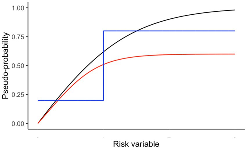
Figure 1. Examples of scaling pseudo-probabilities from a risk variable. Black line is used in the Antarctic krill example below to represent scaling of predation pressure using (h = 3; v = 3; X₅₀ = 0.5; X₀ = 0; X₁ = 4; Y₀ = 0; Y_r = 1). Red line shows similar curvature to the black line but with a maximum value less than one. The blue line shows a threshold scaling, where the importance is at a minimum below the threshold risk and at a maximum above it.

$\mathrm{Y}=Y_0+Y_r\left[\frac{l\left(X\right)-l\left(X_0\right)}{l\left(X_1\right)-l\left(X_0\right)}\right]$

where $l\left(X\right)=\frac{1}{{\left(1+e^{-h\left(X-X50\right)}\right)}^{1/v}}$

$\begin{array}{ll}{Y}_0+Y_r\le 1& (3)\end{array}$

and the symbols are: Y₀ (Y intercept), Y_r (range of Y), X (value of risk to be scaled), X₀ (minimum risk), X₁ (maximum risk), h (steepness), X₅₀ (risk at which half of Y_r is reached), v (shape).

2.1.3. Critical value of the risk index

Once the pseudo-probabilities of the risks relative to fishing level have been determined for a given area, the fishing level in that area could be that at which the resultant risk index is at a satisfactory low level, i.e., a target level, R.. In the first instance, the target level may be determined from the combination of critical levels for each risk, r., such that, using Equation 2:

$\begin{array}{ll}\stackrel{•}{R}=1-\underset{n}{\Pi }(1-{\stackrel{•}{r}}_n)& (4)\end{array}$

Meeting the target level in Equation 4 by reducing some risks may result in other risks being left at too high a level. Care will be needed in how target composite risks are applied.

2.1.4. Region-wide mean risk

The region-wide mean risk is the sum across all areas, a, of the area-specific risk, weighted by the size of areas, A_a, in which the area-specific risk index is assessed. It can be used as a guide to the consequences of different spatially-distributed fishing strategies in the region, including the use of closed areas for moderating risk:

$\begin{array}{ll}\stackrel{\wedge }{R}=\frac{{\Sigma }_a{A}_a{R}_a\left(F_a\right)}{{\Sigma }_a{A}_a}& (5)\end{array}$

We have focussed on heterogeneity of risks in space within the region of a stock for developing the framework. The framework could be further extended for a suite of fisheries with different spatial structures and for when fishing in one area impacts on the ecosystem in other areas (Constable, 2014).

2.2. Using the risk index for spreading risk during developing fisheries

Knowledge on the relationship of many ecosystem risks and the magnitude of fishing is often only coarse (Smith et al., 2007). Nevertheless, a first step for identifying spatial variation in ecosystem properties can be to assess spatial structure in the system from satellite-obtained environmental data (Constable, 2011). This spatial structure can then be refined and potential risks from fishing identified with the addition of field observations, species distribution modelling, dynamic modelling and other tools (Melbourne-Thomas et al., 2017; Brasier et al., 2019; McCormack et al., 2021). We extend the framework above to spread the fishery to reduce risks while the fishery develops and data on risks to the ecosystem from different levels of fishing and its distribution are obtained. The aim is to guide the fishery to have a higher fishing pressure, such as catch density, in lower risk areas than higher risk areas.

2.2.1. Baseline regional risk

First consider the baseline strategy for distributing a developing fishery. Neutral pressure of the fishery on a target stock is to apportion catch in a given area according to the proportion of the target stock in that area. This neutral pressure is then adjusted to account for local area ecosystem vulnerabilities, thereby reducing the fishery in higher risk areas. The resulting distribution is the baseline catch vector with an attendant baseline regional risk to the ecosystem.

Neutral fishing pressure ( ${\dot{F}}_a$ ) is the proportions of the region-wide catch or effort that could be taken from the respective local areas and/or times that result in the same fishing pressure on the target stock in each area. For example, this fishing pressure could be according to the proportions of the stock in each area, determined from the respective measures of density, D, and the surface area of the area, A:

$\begin{array}{ll}{\dot{F}}_a=\frac{D_a{A}_a}{{\Sigma }_{a^{\prime }}{D}_{a^{\prime }}{A}_{a^{\prime }}}& (6)\end{array}$

where a’ refers here and in the following equations to all areas in the assessment.

Equation 2 provides the basis for assessing ecosystem risks and using pseudo-probabilities to assess overall risk from fishing in a local area. As the risk may not be able to be quantified directly in the first instance, we use the term vulnerability, in the interim, to reflect how, for a particular attribute, v_n, one area may vary from another in terms of its vulnerability to fishing (discussed further in the next subsection), such that:

$R=1-\underset{n}{\Pi }\left(1-v_n\right)$

$\begin{array}{ll}\mathrm{where}0\le v_n\le 1& (7)\end{array}$

In this case, vulnerabilities may be ranked differences between areas or some quantitative metric for each area not yet adjusted to risk. In these cases, the metrics will need to be scaled between 0 and 1, such as by using Equation 3.

The equation for determining the proportion, α_a,t (also termed alpha in the text), of catch or effort in each area and time, t, is:

$\begin{array}{ll}{\alpha }_{a,t}=\frac{{\dot{F}}_{a,t}\left(1-R_{a,t}\right)}{{\Sigma }_{a^{\prime },t^{\prime }}{\dot{F}}_{a^{\prime },t^{\prime }}\left(1-R_{a^{\prime },t^{\prime }}\right)}& (8)\end{array}$

where t’ refers here and in the following equations to all time periods in the assessment.

The vector of alphas for all areas in the region is the distribution of catch or effort that spreads the ecosystem risk. The contribution to regional risk of the local area in a time period is the product of α_a,t and R_a,t. The baseline risk to fishing is then the catch or effort weighted risk from across the region, which is the sum of the local area contributions to risk:

$\begin{array}{ll}\widehat{R}={\displaystyle \sum _{a,t}{\alpha }_{a,t}}{R}_{a,t}& (9)\end{array}$

2.2.2. Accounting for preferred fishing patterns

Preferred fishing patterns will likely be different from the baseline alpha vector. The fishing industry may have preferred locations or wish to concentrate on the target species in areas of greatest value, such as greater abundances or areas where schooling occurs naturally and predictably. Other factors may influence fishing; sea ice cover is an important consideration in Antarctica. Areas may not allow fishing such as areas for purposes of biodiversity conservation, recovery of stocks, refugia, or reference areas for scientific or management purposes. A method is needed to take account of these desirable fishing patterns while ensuring baseline risk, $\widehat{R},$ is not exceeded, i.e., by reducing the total catch in the overall region.

The method for accounting for desirable fishing patterns has two steps. The first is to determine an initial alternative catch vector of alphas, ${\alpha }^{\prime }.$ The second step is to modify the vector if the resulting catch-weighted region-wide risk is greater than the baseline risk.

The initial vector ${\alpha }^{\prime }$ could be determined in many ways. One approach would be to develop an index for desirability, D, of the different areas and times in the same way the risk index is developed, but for desirability factors rather than risks, and include this in Equation 8, such that

$\begin{array}{ll}{{\alpha }^{\prime }}_{a,t}^{}=\frac{{\dot{F}}_{a,t}\left(1-R_{a,t}\right)D_{a,t}}{{\Sigma }_{a^{\prime },t^{\prime }}{\dot{F}}_{a^{\prime },t^{\prime }}\left(1-R_{a^{\prime },t^{\prime }}\right)D_{a^{\prime },t^{\prime }}}& (10)\end{array}$

Another approach may be to simply nominate the vector of ${\widehat{R}}^{\prime }$ , if there was an identifiable preference of where to concentrate fishing.

Following Equation 9, the new region-wide risk, ${\widehat{R}}^{\prime }$ , is determined by substituting ${\alpha }_{a,t}$ with ${{\alpha }^{\prime }}_{a,t}^{}$ . If the new region-wide risk is greater than the baseline then strategies need to be employed to reduce ${\widehat{R}}^{\prime }$ until it is less than or equal to $\widehat{R}$ . According to the formulation in this paper, the reduction could be achieved by scaling the catch vector by $\frac{\widehat{R}}{{\widehat{R}}^{\prime }}$ , reducing the overall regional catch. Alternatively, consideration could be given to modifying the catch vector to offset risks by closing high risk areas or the like until equality with the baseline is achieved.

This method for distributing the fishery when only vulnerabilities are known is the focus for the remainder of the paper.

2.2.3. Including closed areas for offsetting risks or conserving biodiversity

Setting fishing to zero in closed areas is one method for offsetting risk before a reduction in overall catch limit. Closing areas of high conservation value is also important for achieving objectives for conserving biodiversity. Incorporating closed areas into the calculations is achieved after the calculation of the baseline catch vector, by modifying each neutral fishing pressure in which there is a closed area (surface area, C) for inclusion in Equation 10:

$\begin{array}{ll}{\dot{F}}_a=\frac{D_a\left(A_a-C_a\right)}{{\Sigma }_{a^{\prime }}{D}_{a^{\prime }}{A}_{a^{\prime }}}& (11)\end{array}$

Care is needed in applying such offsets in order to avoid increasing risks to unacceptable levels for some factors in other areas. The effects of offsets can be determined by examining the risks for individual factors under candidate scenarios, a recommended step in all analyses.

2.2.4. Illustration

A simple example to illustrate this method is given in Table 1 and Figure 2. It has two parts. First, the calculation of the baseline catch vector and the baseline catch-weighted region-wide risk. This shows how the catch is moved away from the high risk areas and added to the lower risk (in this case, no risk) areas. Note, if the risk for any area is equal to 1 then no catch will be taken from those areas. Second, it illustrates how a preferred fishing strategy may result in lower region-wide catches than expected when the region-wide risk under the preferred strategy is adjusted to be no more than the baseline risk. This is because the catch vector needs to not exceed the risk in any one local area.

TABLE 1

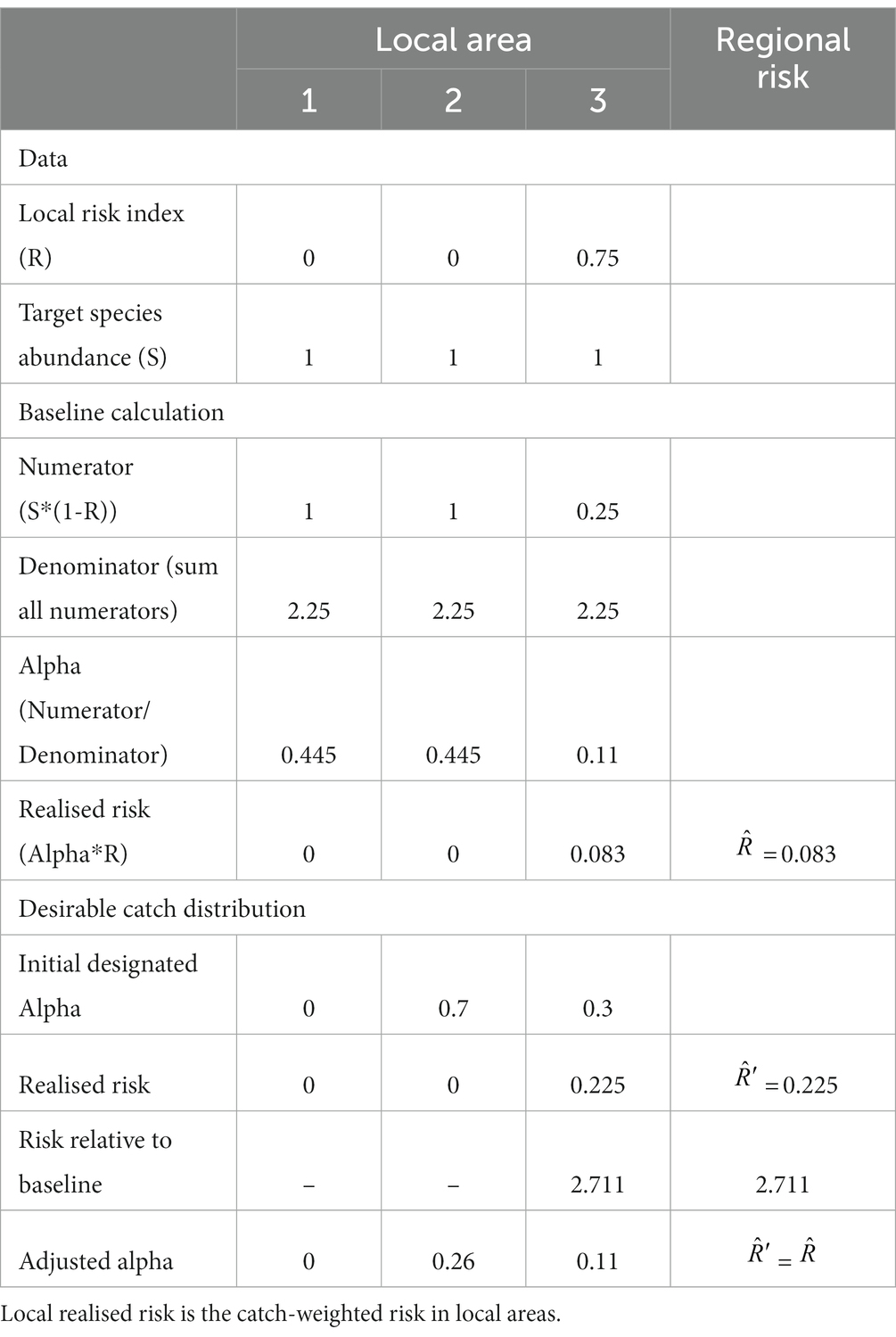
Table 1. Simple example of distributing catch amongst three areas (see Figure 2 for an illustration of the baseline scenario), along with assessment of risk for an example of proposed distribution of catches between areas.

FIGURE 2

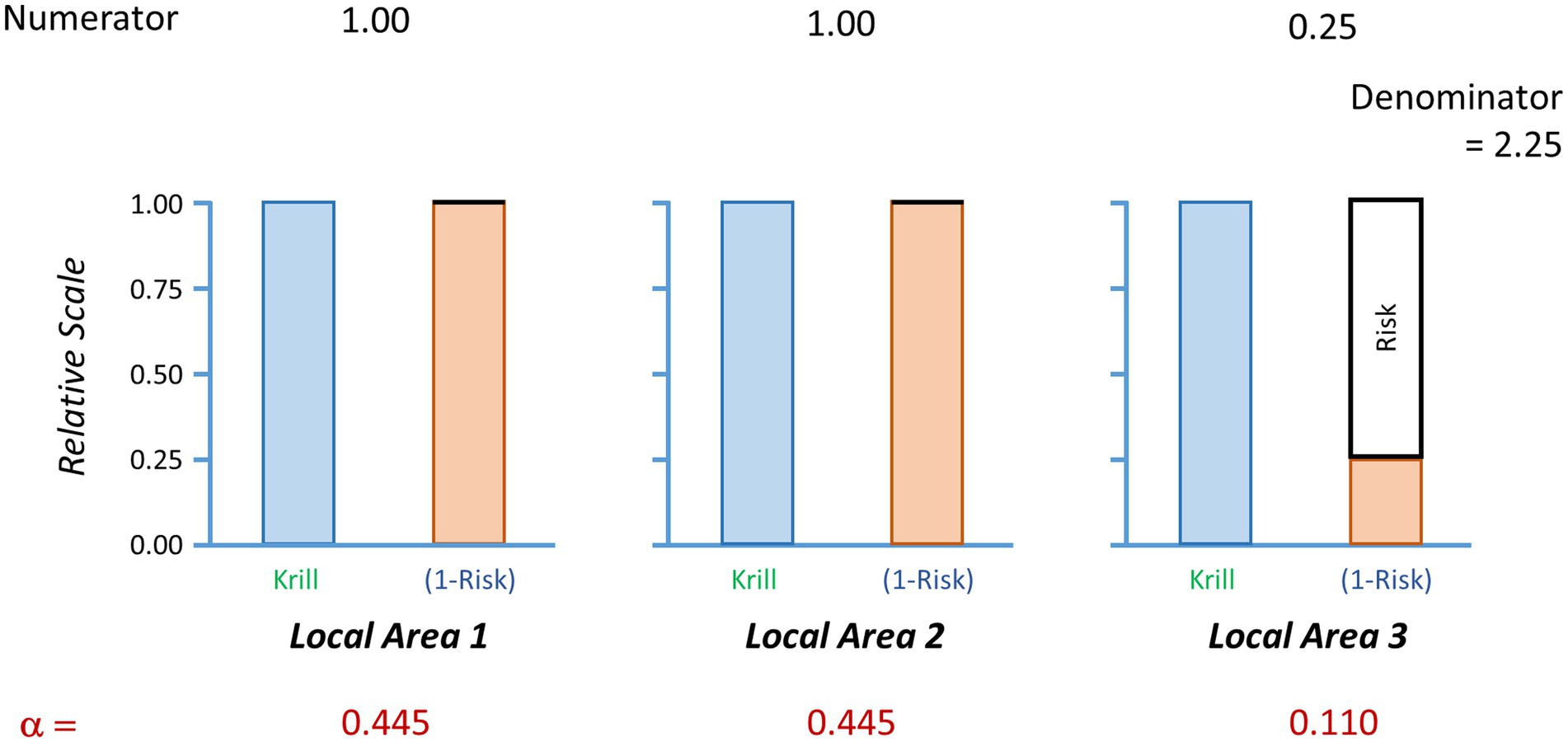
Figure 2. Illustration of the calculations of a baseline catch vector. In this case, the region is divided into three local areas. The ecosystem risks in each local area are shown in the solid black boxes above the orange bars. Local areas 1 and 2 have zero risks while local area 3 has ecosystem risks of 0.75. The target species (blue bars) has the same relative abundance equalling 1 in each local area. The values of the numerator show the multiplication of krill abundance times the value of one minus the risk (orange bars). The denominator is the sum of the values in the numerator. Alpha is the proportion of the regional catch limit to be assigned to each local area. Each alpha is determined by the division of the respective numerator by the denominator. A regional risk is calculated as the sum of the local realised risks, which are the multiplications of alpha times the risk. Here, the baseline regional risk is 0.083 (Table 1).

2.2.5. Accounting for uncertainty

Most inputs will have some degree of uncertainty. Randomisation methods are suitable for estimating a catch vector to distribute the fishery. Two steps are needed: (i) randomise inputs to give a replicate set of baseline catch and local risk vectors across areas, and (ii) use the replicate vectors for establishing a catch vector for the fishery.

The first step is dependent on the values used to develop inputs to the formulae, along with their errors. The approach would be to have a large number of trials, each randomly sampling the values for undertaking the calculations from their respective statistical distributions and then determining the baseline catch vector for a trial. The second step, itself, has two parts. The estimated baseline catch vector for the fishery can simply be estimated as the mean of the replicate baseline catches for each area and ensuring the consequent proportions of the region-wide catch sum to one. Implementation of a preferred option, either wishing to apply the neutral catch vector (as the proportion of the stock in each area) or a specified fishing pattern, may require a downward adjustment of the regional catch.

In order to account for the uncertainty in a preferred option, we suggest the adjustment, if needed, is determined using the following method. First, for each randomisation trial, the regional risk is calculated from the replicate vectors of local risk combined with the estimated baseline catch vector, as well as with the preferred vector, giving replicate values of regional risk for each. As in Section 2.2.2, the adjustment for each trial is calculated as the quotient of the regional risks of baseline over preferred. The median of these adjustments could be used as the overall adjustment of the region-wide catch.

An illustration of this approach is in Table 2 and Figure 3 with the implementation in Supplementary material (SM Table 1). Results in Figure 3D show the estimated baseline catch (alpha) reduces the regional risk distribution across the trials compared to the distribution when the individual trial catch vectors are used, probably from keeping catches lower in many trials. The neutral and specified catch vectors increase the regional risk. In the latter case, the median downward adjustment of the specified catch vector is 0.54.

TABLE 2

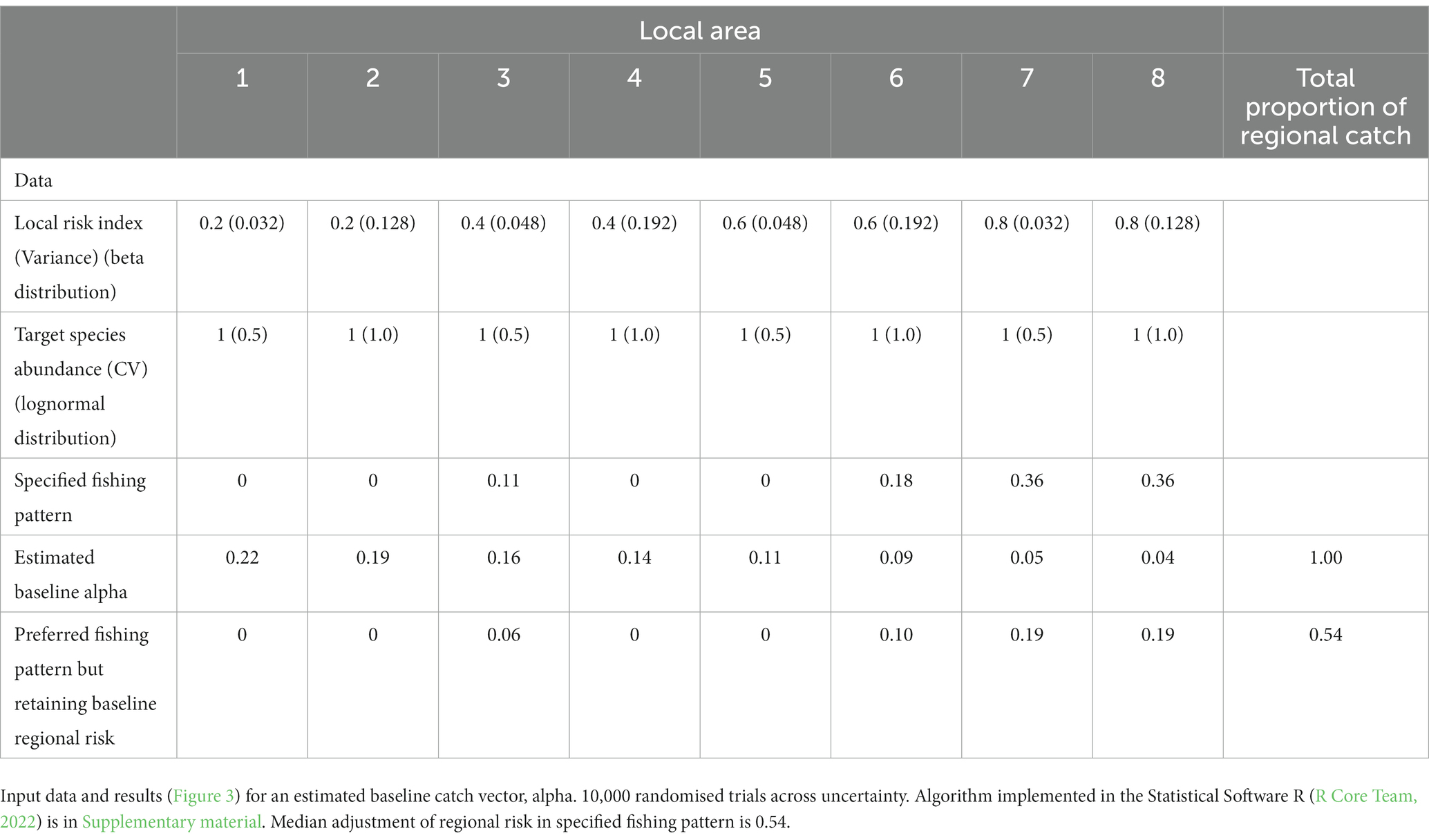
Table 2. Illustration for accounting for uncertainty in spreading risk amongst 8 areas.

FIGURE 3

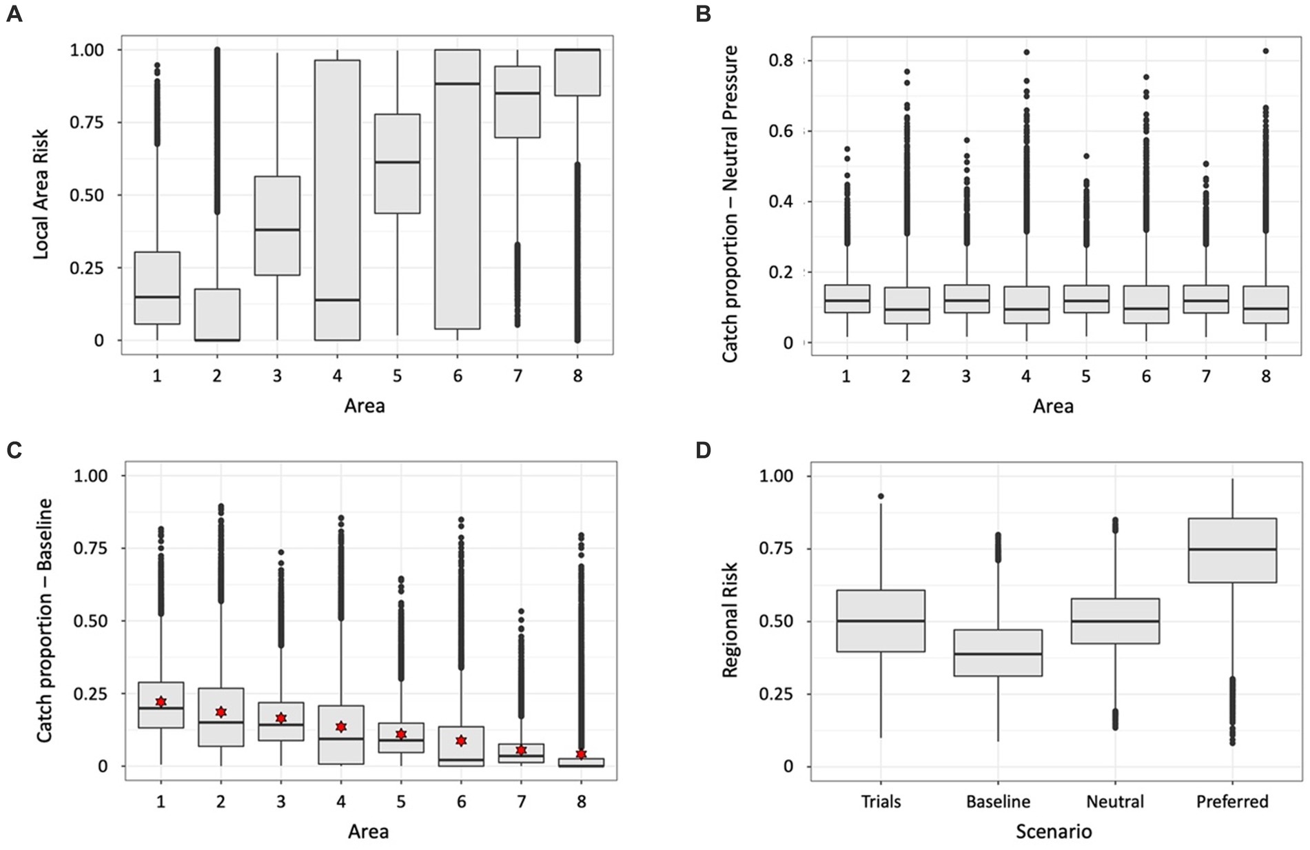
Figure 3. Results of illustration of estimating baseline catch vector by randomising (10,000 trials) across uncertainty, using the input parameters in Table 2. Boxplots showing the distributions across all trials of (A) local area risks in each of the eight illustrative local areas, (B) proportions of catch from each local area under neutral fishing pressure, i.e., the proportion of the target species in a local area, (C) proportion of catch in the baseline catch vectors calculated in each trial – red stars indicate the estimated catch vector for use as baseline, and (D) regional risk, as calculated using the risk vector in each trial combined with the following catch vectors – ‘Trials’ uses the respective catch vectors in each trial, ‘Baseline’ uses the estimated catch vector indicated by the stars in (C), ‘Neutral’ uses the catch vector from proportions of the target species in each area derived using the mean abundances from each area in Table 2, ‘Preferred’ is the vector specified in Table 2.

3. Example: Antarctic krill fishery in FAO Statistical Area 48

An important focus of ecosystem-based management of fisheries (EBFM) is to limit alteration of food webs from the cascading effects of removing target and by-catch species (Fulton et al., 2019), an especially important issue for wasp-waist fisheries where target species are important prey of many predators in the food web (Atkinson et al., 2014). Conserving predators is often not straight forward when predators interact at many different spatial scales relative to the target species, the fishery will often prefer to target the same prey aggregations as the predators, and the expansion of the fishery may be faster than the acquisition of data on the requirements for conserving predators (Constable, 2006).

A staged approach to the development of the fishery is needed for ensuring conservation of predators is achieved while gathering data and developing suitable EBFM strategies (Constable, 2006; Constable, 2011; SC-CAMLR, 2011).

Scientists under the auspices of the Commission for the Conservation of Antarctic Marine Living Resources (CCAMLR) have been considering a precautionary EBFM approach for Antarctic krill predators since its inception, including developing an ecosystem monitoring program (Agnew, 1997), considering approaches to subdivide the krill catch limit for FAO Statistical Area 48 into Subareas (Hewitt and Watters, 1992), determining areas of predator demand for krill as a means of determining areas where predators would be vulnerable to fishing for krill (Agnew and Phegan, 1995), and, since 2001 (Constable, 2001; SC-CAMLR, 2001; Constable, 2002), considering spatial management strategies and the use of spatially structured models to evaluate their ability to manage the food web effects of fishing (Constable, 2004; SC-CAMLR, 2004; Constable, 2005; Watters et al., 2013; Klein et al., 2018). The primary management outcomes for conserving krill predators in CCAMLR has been (i) allowing for escapement of krill to provide for predators in the decision rule used to establish catch limits for krill (Constable et al., 2000) in Conservation Measure 51–01 (CCAMLR, 2021), (ii) establishing in Conservation Measure 51–01 (CCAMLR, 2021) an interim limit, known as the ‘trigger level’, of 620,000 tonnes in Area 48 until a means of subdividing the krill catch into smaller management units has been determined (Constable, 2006), and (iii) subdividing the krill trigger level amongst Statistical Subareas in Area 48 in Conservation Measure 51–07 (CCAMLR, 2021). The latter was established for the 2009 season because of concerns that the trigger level might impact on krill predators if all the catch was concentrated in a small area (SC-CAMLR, 2008a; Watters et al., 2013, 2020). Of note in adopting this Conservation Measure, the Commission reiterated its objectives for krill predators in the preambular paragraphs that:

• “.the need to distribute the krill catch in Statistical Area 48 in such a way that predator populations, particularly land-based predators, would not be inadvertently and disproportionately affected by fishing activity,”

• “.that large catches up to the trigger level from areas smaller than Subareas should be avoided,” and

• “.that the distribution of the trigger level needs to provide for flexibility in the location of fishing in order to (i) allow for interannual variation in the distribution of krill aggregations, and (ii) alleviate the potential for adverse impacts of the fishery in coastal areas on land-based predators.”

Despite this work, there remains no accepted measures for managing the food web effects of fishing at the scale of krill predator populations in CCAMLR. In the absence of being able to set local area catch limits based on local risks of ecosystem effects (Equations 1–5), we use the vulnerability assessment (Equations 7–10) to illustrate how to spread the risk of the krill trigger level. We derive data from historical literature for CCAMLR Statistical Area 48 that has been accepted for use in the Scientific Committee of the Commission for the Conservation of Antarctic Marine Living Resources (Constable et al., 2000; SC-CAMLR, 2006, 2008b, 2016a), and use these in conjunction with updated estimates of krill distribution and abundance in the area (Krafft et al., 2021). Here, we step through the implementation of the method and conclude with available outcomes on risk based on these data.

3.1. Spatial and temporal scales for assessing risk

Antarctic krill, Euphausia superba, is widely distributed in the Southern Ocean (Marr, 1962; Mackintosh, 1972, 1973), with a number of recent reviews describing the factors influencing its distribution, dynamics and long-term change; 70% of the Antarctic krill stock is concentrated between 0°W and 90°W (Area 48), with 87% of the stock over deep oceanic water (>2000 m) (Atkinson et al., 2019; Meyer et al., 2020; Johnston et al., 2022). Biomass estimates at this large geographic scale are derived from three international multi-ship acoustic surveys, undertaken during the summers of 1981 (Trathan et al., 1995), 2000 (Fielding et al., 2011) and 2019 (Krafft et al., 2021). Krafft et al. (2021) reported that while variation in the distribution of krill may occur between years, there is no evidence of a general regional decline in the last 20 years. Smaller, regional acoustic surveys of krill biomass reflect high levels of intra-and inter-annual variability in stock density and biomass, but reveal no trend in abundance (Reiss et al., 2008; Reid et al., 2010; Fielding et al., 2014; Trathan et al., 2022a). However, these surveys do show differences in distribution and biomass between summer and winter (Saunders et al., 2007; Reiss et al., 2017), including with biomass occurring deeper vertically in the water column during winter (Lascara et al., 1999).

The mesoscale distribution of krill is thought to be related to sea ice, shelf bathymetry, and ocean currents, particularly the fronts in the Antarctic Circumpolar Current (ACC) (Johnston et al., 2022) or further south (Trathan et al., 2022a). Although there are no consistent environmental relationships apparent across regions in space and time (Silk et al., 2016), the ACC plays an important role in transporting krill across the region, beginning in the west Antarctic Peninsula and southern Weddell Sea (Hofmann and Murphy, 2004; Thorpe and Murphy, 2022), indicating that the ‘stock’ of krill extends across the south Atlantic, at least to CCAMLR Subareas 48.1, 48.2, 48.3, and 48.4, but probably more extensively.

Risks to predators occur at two main spatial scales within the region of the stock. Land-based predators, such as seals and penguins, operate at local scales near to their breeding colonies, while pelagic predators, such as whales, fish and pack ice seals, are distributed more across the region depending on their feeding grounds (Bestley et al., 2020). Subareas are likely to be insufficient to manage local scale risks. In 2002, the Scientific Committee of CCAMLR determined small-scale management units (SSMUs) in Area 48 to manage local-scale effects of krill fishing (Figure 4; Constable and Nicol, 2002; SC-CAMLR, 2002; Hewitt et al., 2004b). While it is 20 years since those SSMUs were cast and that it is time for their review, they still form a suitable basis on which to consider how to spread risk and conserve predators at their ecologically-relevant scale.

FIGURE 4

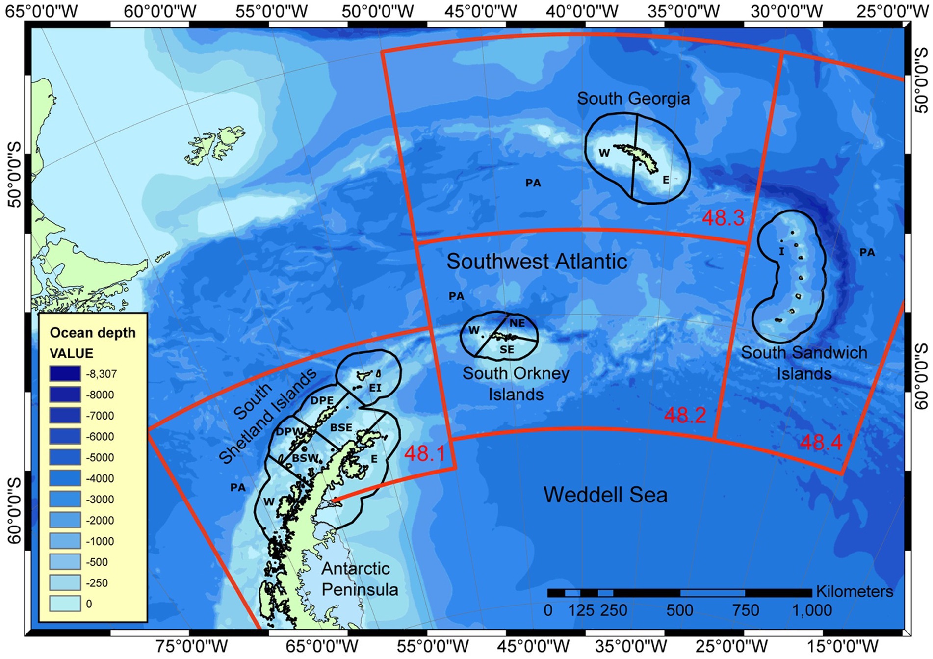
Figure 4. Small-scale management units in FAO Statistical Area 48 established by the Scientific Committee of CCAMLR in 2002 (SC-CAMLR, 2002). FAO Subareas (numbers shown in red) are 48.1 (Antarctic Peninsula, AP), 48.2 (South Orkney, SO), 48.3 (South Georgia, SG) and 48.4 (South Sandwich, SS). Small-Scale Management Units are shown with acronyms relating to the Subareas: PA, Pelagic Area; E, East; NE, North East; SE, South East; W, West; BSE, Bransfield Straight East; BSW, Bransfield Straight West; DPE, Drake Passage East; DPW, Drake Passage West; EI, Elephant Island; I, Islands. Full acronym for an SSMU used in later figures and tables have the Subarea acronym as the first two letters combined with the relevant SSMU acronym used here.

The time-period for the application of a catch limit is the overall temporal scale of the assessment, usually 1 year. For polar regions, there is extreme seasonality giving rise to production occurring in spring and summer and stasis or attrition in autumn and winter. This is exemplified by many life histories. For example, whales and many seals migrate to the north of the Antarctic region in winter and many predators tied to land in summer during the breeding season will forage more widely and away from their colonies in winter (Bestley et al., 2020).

Individual krill live for a number of years, with a plausible maximum age of around six-plus (Quetin and Ross, 2003). Somatic growth is seasonal, with an increase in body size during spring and summer with possible shrinkage over winter (Ikeda, 1985; Constable and Kawaguchi, 2017). Observations suggest winter shrinkage is most apparent in adult females but not males, based on the tracking of modal size classes over seasons and sex-ratio patterns; other explanatory factors, such as differential mortality, immigration and emigration, do not explain the observed differences (Tarling and Fielding, 2016). Growth rates are thought to be greater where primary production is higher, but with limitations imposed by sea ice and sea surface temperature (e.g., with elevated growth in spring around South Georgia; Murphy et al., 2017).

The risks to krill and predators from krill fishing are therefore not the same throughout the year. Here, we divide the year into two seasons, summer and winter, to take account of this variation and compare this to an assessment without considering season.

3.2. Neutral fishing pressure for krill

Neutral fishing pressure for krill was determined from the proportion of biomass in each area. Densities of Antarctic krill were derived from the results of two regional surveys in austral summer of Area 48: 1999–2000 (Watkins et al., 2004; Hewitt et al., 2004a) and 2018–2019 (Krafft et al., 2021). The two surveys have been analysed using the same stratification (Table 3a), with island strata (areas near to the islands) in each of Subareas 48.1 (South Shetlands), 48.2 (South Orkney), 48.3 (South Georgia), 48.4 (South Sandwich), and larger pelagic strata encompassing much of the remainder of the Subareas.

TABLE 3

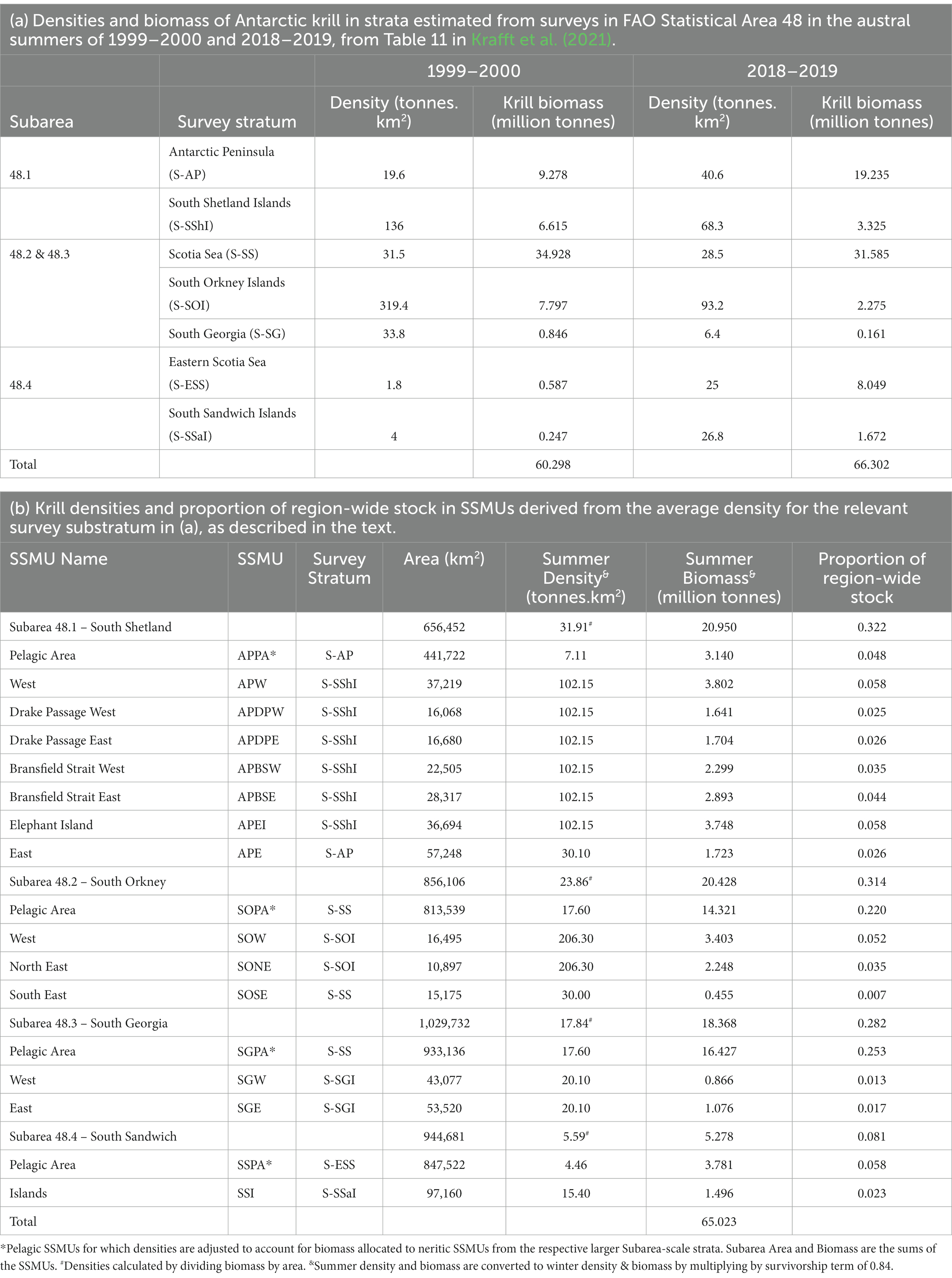
Table 3. Derivation of densities of Antarctic krill for small-scale management units (SSMUs) in FAO Statistical Area 48 and consequent proportions of the region-wide biomass in each SSMU for use in the risk assessment.

Hewitt et al. (2004a) used the densities in the island strata to represent densities in each of the neritic (non-pelagic) SSMUs. In their paper, the pelagic SSMUs were given the densities of the pelagic strata in the surveys. That approach for neritic SSMUs was used here, taken as the mean density from across the two surveys in the relevant island survey strata. The Antarctic Peninsula East SSMU was not surveyed in either survey. The density in Antarctic Peninsula East was approximated as the mean density of the Antarctic Peninsula stratum from across the two surveys. In the South Orkneys, the island stratum encompassed the neritic SSMUs of South Orkney Islands West and North East. The South East SSMU had the mean density of the pelagic stratum applied because of the substantial difference of this stratum to the other neritic strata (Krafft et al., 2018).

In order to ensure the biomass in a Subarea was consistent with estimates from the surveys, the biomass in the respective pelagic SSMUs was calculated as the mean biomass in the Subarea from across the two surveys less the summed biomass from the neritic SSMUs in that Subarea, excluding the Antarctic Peninsula East SSMU. Note the Scotia Sea stratum encompasses Subareas 48.2 and 48.3, which was accounted for in this formulation.

The derived krill densities for each SSMU and the Subareas are given in Table 3b (see also Figure 5), along with the spatial areas of each, and the consequent biomass and proportion of the region-wide stock found in each area.

FIGURE 5

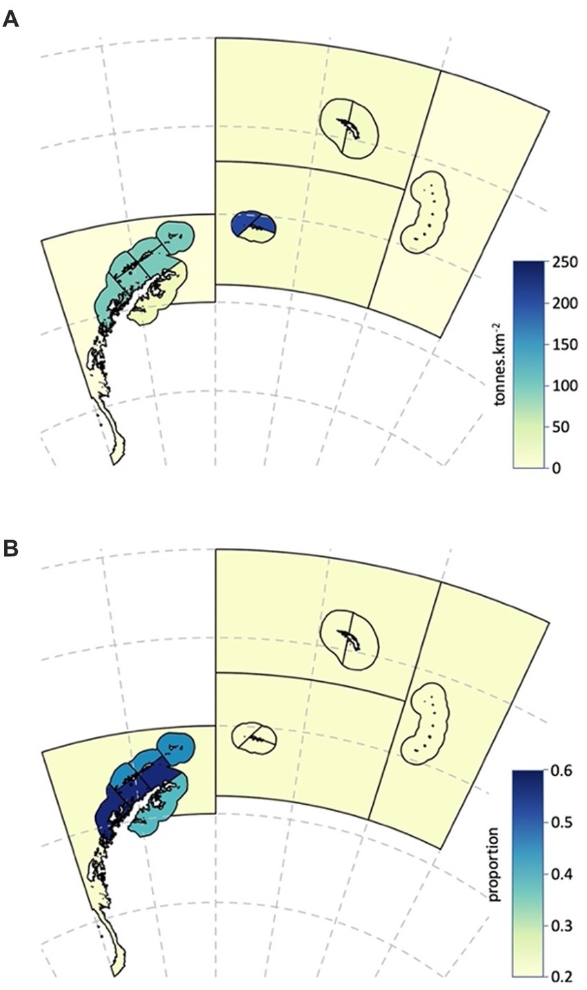
Figure 5. Spatial characteristics of the Antarctic krill population used in the risk assessment. (A) Densities of Antarctic krill (tonnes.km⁻²). (B) Median annual proportion of Antarctic krill less than 35 mm in length in the population.

At present, there are no consistent estimates tracking biomass within SSMUs from summer to winter. In order to partition the year into two seasons, krill densities in winter were approximated from applying constant mortality (M = 0.8 yr⁻¹) (Constable and de la Mare, 1996) giving an average biomass over winter months (May to October) of approximately 0.84 of the average over the summer months (November to April) (Constable, 2000). While this is only an approximation in the absence of other data, we multiply the summer estimates of density/biomass by 0.84 to reflect a difference in winter density/biomass.

3.3. Vulnerabilities of krill

Risks to Antarctic krill from fishing relate to the importance of areas as source areas for adults and recruitment areas for juveniles.

Advection is considered to play a central role in distributing krill across Area 48 with the Antarctic Peninsula being an important source area for krill that then move with the Antarctic Circumpolar Current along the Scotia Arc to the east. Areas where juveniles recruit follow this pattern. While early life stages may be present in most areas where krill are found (Meyer et al., 2020), the population is dependent on successful recruitment, which occurs primarily in the Antarctic Peninsula with advection from this Subarea to the other Subareas (Reiss, 2016).

Spawning is episodic, with multiple spawning events within a year (Quetin and Ross, 2003). Recruitment is episodic and regional, with models showing that the seasonal location of sea ice is the main limiting factor for successful larval recruitment (Thorpe et al., 2019). Spawning in January leads to the greatest extent of viable larval recruitment habitat, while later spawning in February, when sea ice is at a minimum, generally provides insufficient time for larvae to reach a viable developmental stage before the winter sea ice advances (Thorpe et al., 2019).

Generally krill exist within different aggregation states, with swarms, layers and individuals, but with the numbers and sizes of swarms in an area changing across space and time. Smaller, more widely dispersed swarms occur in summer, whilst larger, more infrequent swarms occur in winter, with the patterns and seasonal changes unlikely to be simply the consequence of oceanographic circulation (Lascara et al., 1999). Other behavioural aspects of krill life history also challenge our understanding; for example, it has been observed, at least along the west Antarctic Peninsula, that the length frequency distributions of krill collected by nets exhibits an across-shelf pattern of larger (>40 mm) krill located offshore smaller krill (<38 mm) in all seasons except winter. Such data, coupled with historical observations suggest that there is a seasonal shift in the primary habitat of krill and that changes in behaviour are an important factor in krill distribution. Similar assortative length frequency patterns are also evident within individual swarms, where differences in size between adjacent swarms are probably due to a length-dependent sorting mechanism that restricts the size range of krill in a swarm (Watkins, 1986).

The geographic domain that encompasses the life cycle of krill is unclear. However, deep water is thought to be a prerequisite for successful spawning (Hofmann and Hüsrevoğlu, 2003), as eggs need at least 700 m water depth to fulfil their development before the larvae rise again to the sea surface (Hofmann and Hüsrevoğlu, 2003; Thorpe et al., 2019). Temporal and spatial coherence in patterns of early life-history stages are evident across the Atlantic sector (Perry et al., 2019); however, mechanisms whereby adult life-history stages migrate back onto the shelf after spawning (Siegel, 1988) remain uncertain, particularly given regions of complex bathymetry and strong ocean currents. Transport in oceanographic currents has certainly been a topic of much debate (Renner et al., 2012). Nevertheless, understanding how krill behaviour, recruitment, and movement in ocean currents interact remains elusive, but a key challenge for understanding ecosystem functioning.

Resolving these issues will help increase understanding about the potential for some areas to act as krill sources, or krill sinks. So far, several studies have already begun to consider the complexity of krill movement in relation to local oceanography within the southwest Atlantic, and particularly along the west Antarctic Peninsula region. For example, Capella et al. (1992) reported that the Bransfield Strait and the South Shetland Islands receive krill larvae from the Bellingshausen Sea to the west, the Weddell Sea to the east and from north of the South Shetland Island arc (Figure 4; see also Trathan et al., 2022b). Subsequently, Piñones et al. (2011, 2013a), calculated residence times for biological hotspots using a Lagrangian model, inferring that particle (=krill) retention was aided by certain physical features, including proximity to deep depressions and shelter from wider shelf circulation. Piñones et al. (2013b) and Capella et al. (1992) noted that off-shelf transport from the west Antarctic Peninsula supports the hypothesis that spawning contributes to populations downstream across the southwest Atlantic. Further, age-dependent sea-ice associated behaviour may be important in the transport and distribution of krill populations (Thorpe et al., 2007). Diel vertical migration (DVM) over a 24 h period may also have implications for krill availability. However, Piñones et al. (2013b) noted that DVM made little (< 10%) difference in the horizontal and vertical dispersion of particles.

The relative importance of SSMUs for recruiting krill juveniles is reflected by the proportion of the population in an area comprising animals less than 35 mm in length, the length being sufficient to encompass animals in Year 1 (de la Mare, 1994). The U.S. AMLR program provides a time series of length frequency data from regular surveys in Subarea 48.1, data from which these proportions can be derived.¹ We use the surveys in early summer (January–February; Leg 1) for the period 1996 to 2011 to calculate the proportion of the population in their strata that comprise juveniles. The importance of an SSMU as a recruitment area is determined as the median of the time series of observations from the survey stratum in which the SSMU resides (Table 4 and Figure 5). Juvenile krill have been observed in the other Subareas but only sporadically (e.g., Krafft et al., 2018). For this reason, we apply a recruitment value from the Antarctic Peninsula Pelagic SSMU to the SSMUs of the other Subareas.

TABLE 4

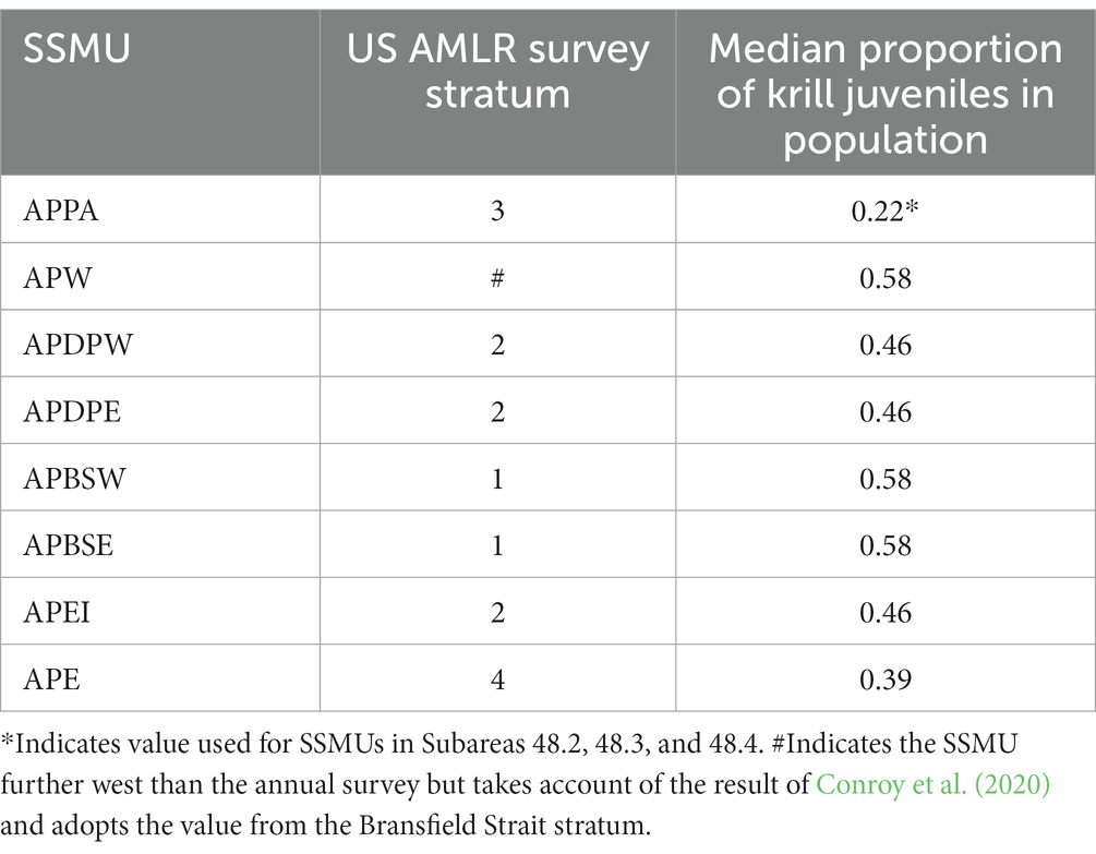
Table 4. Median annual proportion of Antarctic krill less than 35 mm in length in the population in Antarctic Peninsula SSMUs derived from time series of length frequencies in survey strata from early summer by the US AMLR program from 1996 to 2011.

3.4. Vulnerabilities of krill predators

Risks to krill predators include the removal of krill from feeding grounds and the potential disruption of krill availability to predators.

A broad guild of predators feed on krill (Croxall et al., 1985; Trathan and Hill, 2016), made possible by its wide geographic distribution and its various aggregation states. A corollary of this is that krill swarm structure is also thought to be a fundamental response for avoiding predation, whilst krill themselves continue to mate, spawn and feed (Tarling and Fielding, 2016). The dominance of smaller krill swarms in summer along the west Antarctic Peninsula (Lascara et al., 1999) coincides with the feeding activity of numerous central-place foraging seabirds and seals provisioning offspring. The reduction in this concentrated foraging pressure after these land-based predators complete breeding also coincides with the emergence of larger krill swarms in autumn and winter (Lascara et al., 1999). As such, the interplay between predators and krill may be important, even though the actions of individual predators might be relatively minor, the cumulative impacts of many predators may generate significant effects on local prey aggregation states. In this context, the recovery of baleen whales after historical over-exploitation might now have implications for krill aggregation states, given baleen whales feed in differing ways to those of penguins and seals.

Further, there is now also growing recognition that the demands made by land-based predators are likely to be eclipsed by other taxa (Hill et al., 2007; Warwick-Evans et al., 2022). Currently, a number of humpback whale stocks are thought to be close to pre-exploitation levels (Cooke, 2018c), yet other baleen whale species remain well below historical numbers (Cooke, 2018a; Cooke, 2018b). As these also recover, competitive effects are likely to change as species endeavour to re-occupy their historical niches, although whether such niches now remain the same is uncertain, given ecological change (Nicol et al., 2010; Atkinson et al., 2019; Constable et al., 2022). Certainly, in recent years, some penguin species have shown shifts in population abundance, the causes of which have been attributed to climate, but which may equally be (at least partially) a result of changes in inter-specific competition for krill (Ainley et al., 2007; Trivelpiece et al., 2011). Determining how predator dominance changes as baleen whales recover, will be a key topic for future research.

Central-place foraging predators are constrained by the need to provision offspring during the summer breeding season (Figure 6). However, other predators considered to have an ideal-free distribution (Fauchald, 2009), such as baleen whales, fish and squid are not so constrained and so are more likely to track shifting prey resources. Outside the breeding season, central-place foragers are also no longer constrained and may go to regions with more abundant or predictable prey resources. This means that there are distinct spatial patterns of consumption which are predictable within and between years (Trathan et al., 1998; Warwick-Evans et al., 2018, 2019). However, in addition to apparent spatial differences in consumption, all krill-dependent predators also show temporal patterns of consumption across the annual cycle. For example, macaroni penguins, Eudyptes chrysolophus, show different profiles of demand during the year compared with Antarctic fur seals, Arctocephalus gazella, (Boyd, 2002), whilst within a given species, different demographic categories can show subtly different annual profiles across the year (e.g., Adélie penguins, Pygoscelis adeliae – Southwell et al., 2015). Baleen whales may also have different periods of feeding intensity, with particularly hyperphagic periods when they first return to their summer feeding grounds (Baines et al., 2022).

FIGURE 6

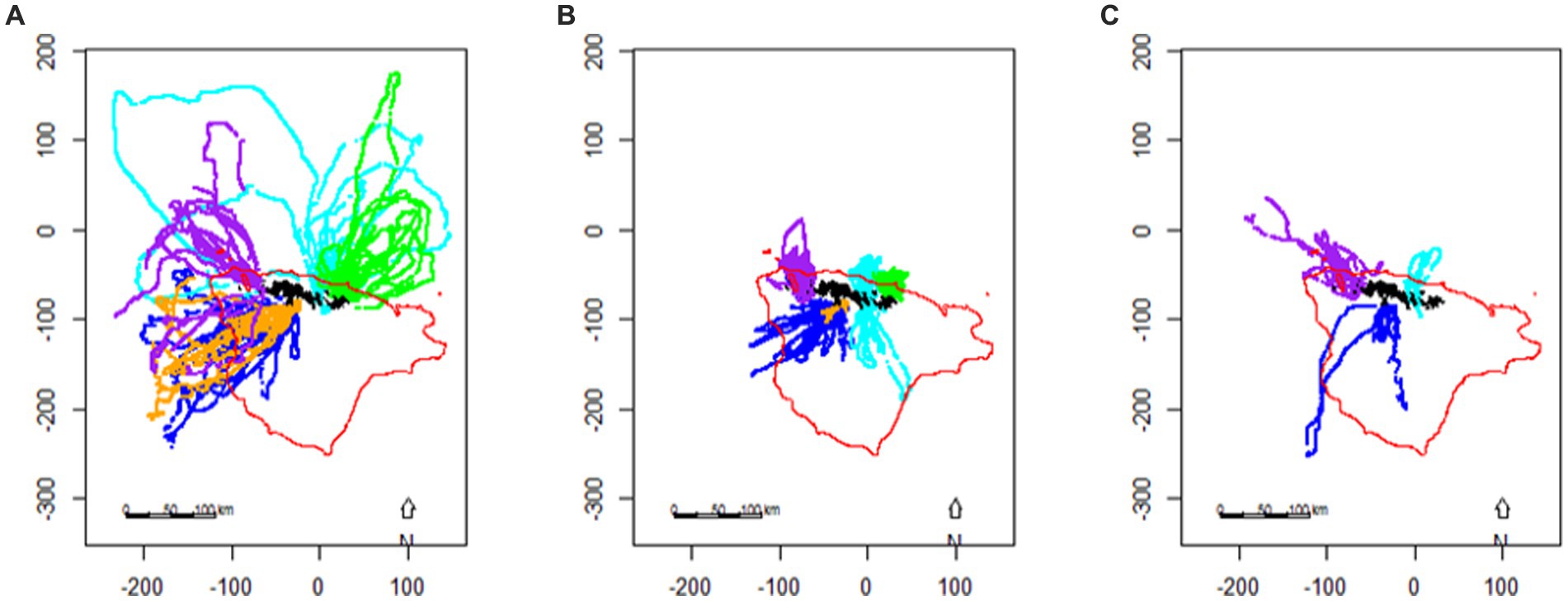
Figure 6. The location of foraging dives made by chinstrap penguins, Pygoscelis antarctica, breeding on the South Orkney Islands during (A) incubation, (B) brood, and (C) crèche based on telemetry data (from Warwick-Evans et al., 2018), axes are shown with units of km (see Figure 4 for location). Colours represent different sites/years: Powell Island (pale blue), Monroe Island (purple), Laurie Island (green), Signy Island 2013 (orange), and Signy Island 2015 (blue). The 500 m isobath, representing the shelf-edge, is indicated in red.

While clear examples exist of spatial overlap between the fishery and various predators (Trathan et al., 2018; Warwick-Evans et al., 2018; Trathan et al., 2022b), there is no evidence as yet on the potential for fishing to interfere with the local availability of krill to predators. Predators have a variety of feeding behaviours, probably arising from the variable aggregation states of krill. Some predator species may feed off individual krill, some skim, whilst some lunge and require krill swarms to feed efficiently. Removal of krill by fishing vessels, or disturbance so that swarm-structure is disrupted into a different aggregation state may displace predators from preferred predictable areas. However, to date little work has been undertaken to assess predator (or fishery) krill aggregation preferences, but the fact that vessels periodically move (SC-CAMLR, 2016b Annex 6, paragraphs 2.215 to 2.221; Santa Cruz et al., 2018) suggests that the potential exists for disturbance competition.

3.4.1. Spatial distribution of krill predation

Predator demand for krill is a product of the abundance of a population (colony) and the per capita consumption of the population. The distribution of predator demand for a population will vary between times of year and between years, particularly for species tied to colonies during breeding, and will depend on the foraging behaviour of the species.

The average annual density (tonnes.km⁻²) of predator demand for krill in small areas was developed from Hill et al. (2007), given the publication of the per annum estimates of summer demand by SC-CAMLR (2011); see Annex 4, Table 3. The winter and summer demand was estimated for all predators combined (fish, whales, fur seals and penguins) in each small-scale management unit according to the parameters and calculations of Hill et al. (2007). Krill-eating fish included in those calculations were nototheniid and channichthyid species in the on-shelf areas and myctophid species in off-shelf areas. Hill et al. (2007) provide the details of these calculations. Table 5a gives the population size of fish, whales, penguins and fur seals in each SSMU along with per capita consumption of krill (g) in each SSMU for summer and winter.

TABLE 5

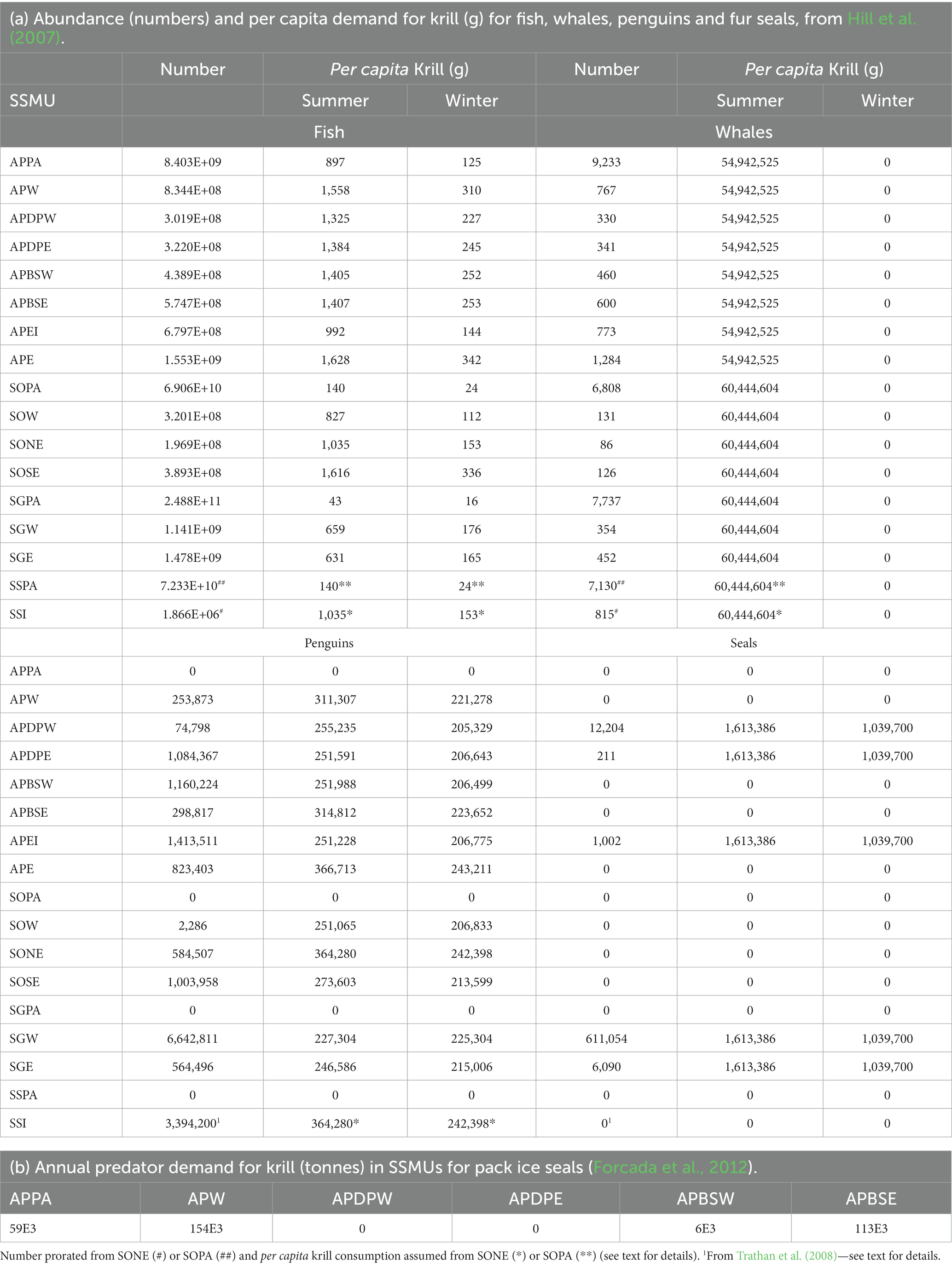
Table 5. Data for calculating predator demand for krill.

The data to calculate predator demand for the SSMUs in Subarea 48.4 were not available except as provided by Trathan et al. (2008) for the numbers of penguins. Trathan et al. (2008) provide a census of fur seal pups, showing only a low abundance of seals on the islands. Without an estimate of abundance of adults, the population of seals was assumed to be zero. For the purposes of developing this example of the risk assessment, we approximated the abundance of whales and fish using proxy methods. The densities of mesopelagic fish and the general attributes of the ocean environment are of similar characteristics between Subarea 48.2 and the area around the South Sandwich Islands (Dornan et al., 2022). We therefore applied the same density of fish and whales in the pelagic and north east SSMUs in Subarea 48.2, along with the consumption rates, to the pelagic and island SSMUs, respectively, in Subarea 48.4. For penguins, we applied the consumption rates from the north east SSMU in Subarea 48.2.

Annual krill consumption by pack ice seals in the SSMUs of Area 48 are available in Forcada et al. (2012) (Table 5b). These are included in the calculations of total predator demand by allocating 60% to summer and 40% to winter, following the partition of demand by fur seals between summer and winter.

These calculations do not include the consumption of krill by flying seabirds. Warwick-Evans et al. (2022) show that flying seabirds consume ~2% during summer around the Antarctic Peninsula. Methods for including flying seabirds in future calculations will be important as predator demand is currently underestimated.

3.4.2. Risks

For Antarctic krill predators, fishing will have the highest risk in areas where there is naturally greater pressure for krill. Predation pressure is the ratio of the predator demand density for krill and the available krill density in an area, i.e., an indicator of the potential for competition amongst predators. Areas with higher predation pressure would be expected to be more vulnerable to the effects of fishing than areas with lower pressure. Here, we evaluate predation pressure for land-based predators and other predators that are more likely to forage according to an ‘ideal-free’ distribution. Data in Tables 3b, 5 are used to calculate predation pressure in each SSMU (Table 6 and Figure 7). Note that winter predation pressure is based on summer krill densities adjusted for expected survivorship after 6 months (Table 3b). The annual predation pressure is an average of the summer and winter pressures.

TABLE 6

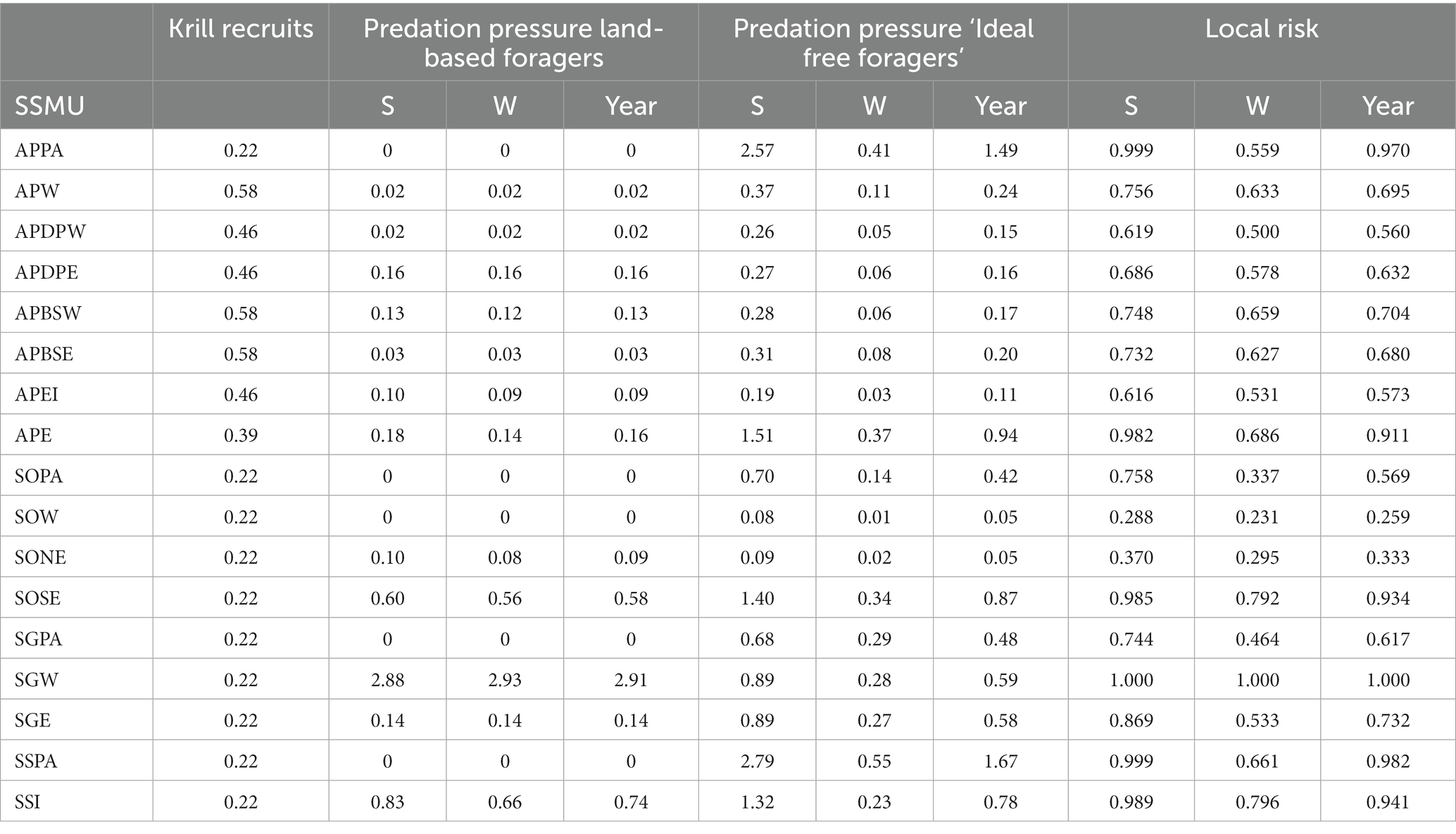
Table 6. Vulnerabilities (krill recruitment and predation pressures) and consequent local area risk in each SSMU for a ‘whole year’ assessment and an assessment with seasons – summer (S) and winter (W).

FIGURE 7

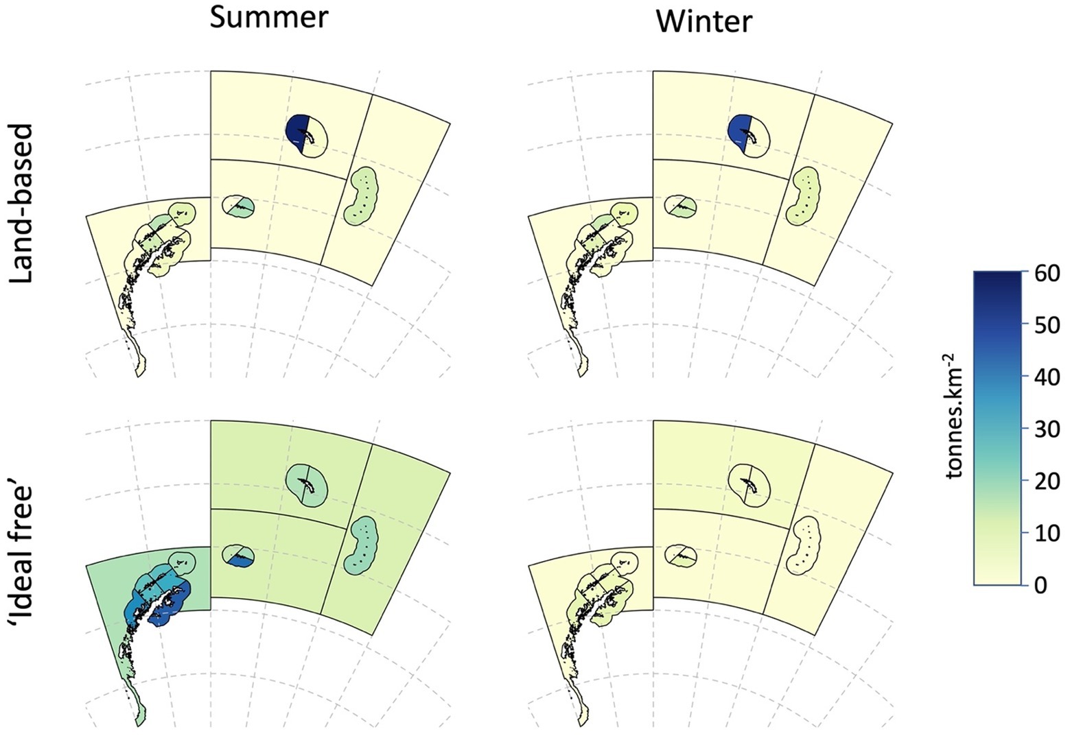
Figure 7. Demand density for Antarctic krill (tonnes.km⁻²) in summer and winter, aggregated for land-based predators and predators that are likely to concentrate foraging in areas of higher densities of krill, termed ‘ideal-free’ foragers.

3.5. Baseline catch distribution and region-wide risk

Baseline Alphas as proportions of the catch limit and the consequent baseline region-wide risks were calculated for two examples: local catches distributed across the SSMUs (i) for the whole year, and (ii) for when the fishery is separated into summer and winter. These examples applied Equations 6–8. The examples developed here are provided in an Excel spreadsheet in Supplementary Material Table 2.

The local risks, $R_{a,t}$ , arising from applying Equation 7 are presented in Table 6 for the two examples, along with the data on the three vulnerabilities – krill recruits, and predation pressure for each of land-based predators and ‘ideal free’ foragers. Krill recruits remained unscaled. Predation pressure was scaled between 0 and 1 using the logistic function in Equation 3 (h = 3; v = 3; X₅₀ = 0.5; X₀ = 0; X₁ = 4; Y₀ = 0; Y_r = 1,illustrated as the black line in Figure 1).

The neutral fishing pressure, ${\dot{F}}_{a,t},$used for calculating the baseline alpha levels, ${\alpha }_{a,t},$ (Equation 8) is the proportion of the region-wide stock in each SSMU shown in Table 3b. The Baseline Alphas for the two examples are presented in Table 7.

TABLE 7

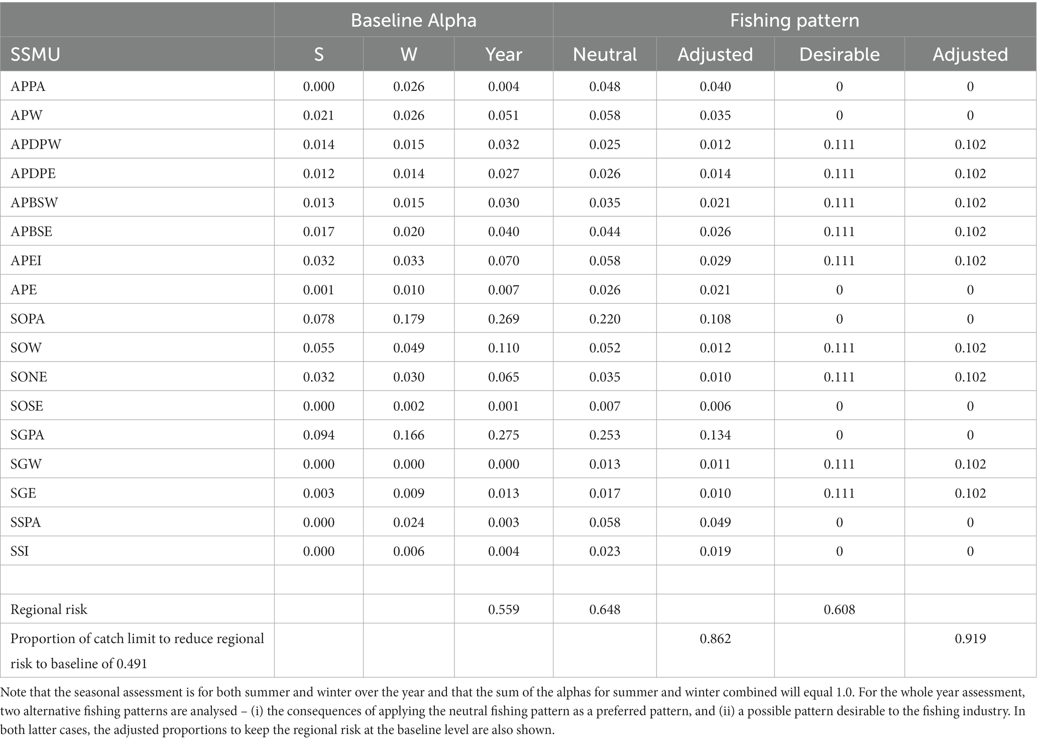
Table 7. Baseline Alpha (proportion of total catch limit) for each SSMU for a ‘whole year’ assessment and an assessment with seasons – summer (S) and winter (W).

The local risks and baseline alphas for the whole year example and for the summer-winter examples are illustrated in Figure 8. The baseline regional risk (Equation 9) for the whole year assessment was 0.559 (Table 7).

FIGURE 8

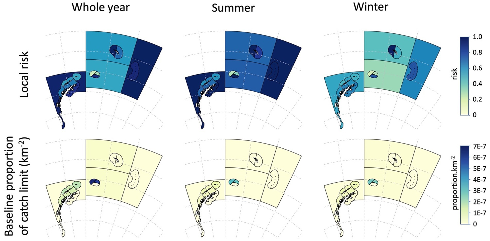
Figure 8. Local risk in each assessment area (Table 6) and the baseline proportion of the catch (alpha) (Table 7) displayed as proportion per km² for the whole year, and for the seasonal assessment splitting the year into summer and winter (see Table 7 and the text for details).

3.6. The krill fishery and managing preferred fishing patterns

The vast majority of the krill stock occurs in deep oceanic water but is unpredictable in location and often at low density in this habitat (Figure 5). Therefore, over time, the fishery has coalesced into areas where krill are more predictable and at levels of abundance that are desirable to fishery operators. These areas tend to be over shallower shelf waters, or at the shelf edge, such that the fishery now generally operates close to island archipelagos within the southwest Atlantic (Santa Cruz et al., 2018). Recent studies have highlighted the potential for the krill fleet to locally deplete levels of krill (or disturb the swarm structure) such that vessels relocate, with catch rates per hour in fishing hotspots gradually declining over four or 5 days (SC-CAMLR, 2016b Annex 6, paragraphs 2.215 to 2.221). Such a result highlights the potential for the fishery to compete with predators. At these scales of operation, managers need to understand the critical levels of krill density preferred by different predators, and the time taken for an area to recover to a given density level after depletion (Trathan et al., 2022b).

We illustrate how to manage preferred fishing patterns if the baseline alphas do not seem satisfactory. First, we examine the unweighted fishing pattern of neutral fishing pressure based on krill densities might be managed. Table 7 shows how the regional risk (Equation 9) is increased to 0.648, greater than the baseline risk of 0.559. The proportion of catches in each SSMU need to be adjusted downward by 0.138 in order to retain the regional risk at the baseline level. The second scenario was for a pattern with a desirability of the fishery to operate around the Antarctic Peninsula and adjacent to islands. In this case, we set equal catches to be taken from the SSMUs near to land (Table 7). The consequent regional risk is 0.608, requiring an adjustment of catches downwards by 0.081 to satisfy the baseline risk.

4. Concluding remarks

The risk assessment procedure presented here provides a method for combining risks to conservation from fisheries into a single metric and to use this to identify areas of higher overall risk. The procedure then has mechanisms to spread the fishery away from higher risk areas, to adjust catch limits to reduce risks if the fishery cannot avoid such areas, and to also allow for closed areas to help compensate for higher risks in other areas. It also includes the rationale for how adjustments to fishing patterns can be implemented to appropriately spread risks arising from fisheries when a full risk assessment is not possible. We used the Antarctic krill fishery as a case study but this framework can be readily applied to other fisheries. The method allows for the seamless inclusion of new data when they become available, but can be implemented with existing data. A further feature of this method is that the risk of impacts can be assessed for individual areas of interest based on more detailed information for that area whilst including it in a wider assessment across many areas, thereby enabling broader ecological considerations to be incorporated. In conclusion, spatial ecosystem-based management strategies for fisheries can proceed from the outset of a fishery using suitable proxies for ecosystem vulnerabilities within a risk framework.

Data availability statement

The original contributions presented in the study are included in the article/Supplementary material (Table 1 - code for undertaking the uncertainty simulation; Table 2 - the data and working of the Antarctic krill fishery example), further inquiries can be directed to the corresponding author.

Author contributions

AC conceived of the project, developed the framework, undertook the simulations, and led the writing of the manuscript. SK, PT, and VW-E contributed to detailing the Antarctic marine ecosystem, trialling the framework, and writing the manuscript. MS contributed to analytical support and mapping. All authors contributed to the article and approved the submitted version.

Funding

AC, SK, and MS were supported by the Australian Antarctic Division. AC was also supported by the Australian Cooperative Research Centre program through the Antarctic Climate and Ecosystems Cooperative Research Centre, and through a Pew Fellowship in Marine Conservation. VW-E was funded through Darwin Plus (grant DPLUS072) and the Pew Charitable Trusts (grant no. PA00034295). PT was funded through the NERC BAS-ALI Science budget, with a collaborative study trip to Hobart funded by the Pew Charitable Trusts (grant no. PA00034295).

Acknowledgments

Thanks to many colleagues in the Scientific Committee for the Conservation of Antarctic Marine Living Resources who contributed to many discussions through 2016, based on the original paper (WG-EMM-16/69). Thanks also to Bill de la Mare, Jess Melbourne-Thomas, and Rowan Trebilco for stimulating discussions on the application of risk methodologies in fisheries and ecosystem management. Thanks to many colleagues in the Australian Antarctic Division and the Antarctic Climate and Ecosystems Cooperative Research Centre for discussions and reviewing the original manuscript submitted to WG-EMM.

Conflict of interest

The authors declare that the research was conducted in the absence of any commercial or financial relationships that could be construed as a potential conflict of interest.

Publisher’s note

All claims expressed in this article are solely those of the authors and do not necessarily represent those of their affiliated organizations, or those of the publisher, the editors and the reviewers. Any product that may be evaluated in this article, or claim that may be made by its manufacturer, is not guaranteed or endorsed by the publisher.

Supplementary material

The Supplementary material for this article can be found online at: https://www.frontiersin.org/articles/10.3389/fevo.2023.1043800/full#supplementary-material

Footnotes

1. ^KRILLBASE at https://doi.org/10.5285/8b00a915-94e3-4a04-a903-dd4956346439

References

Agnew, D. J. (1997). The CCAMLR ecosystem monitoring programme. Antarct. Sci. 9, 235–242. doi: 10.1017/S095410209700031X

CrossRef Full Text | Google Scholar

Agnew, D. J., and Phegan, G. (1995). Development of a fine-scale model of land-based predator foraging demands in the Antarctic. CCAMLR Sci. 2, 99–100.

Google Scholar

Ainley, D., Ballard, G., Ackley, S., Blight, L. K., Eastman, J. T., Emslie, S. D., et al. (2007). Paradigm lost, or is top-down forcing no longer significant in the Antarctic marine ecosystem? Antarct. Sci. 19, 283–290. doi: 10.1017/s095410200700051x

CrossRef Full Text | Google Scholar

Atkinson, A., Hill, S. L., Barange, M., Pakhomov, E. A., Raubenheimer, D., Schmidt, K., et al. (2014). Sardine cycles, krill declines, and locust plagues: revisiting ‘wasp-waist’ food webs. Trends Ecol. Evol. 29, 309–316. doi: 10.1016/j.tree.2014.03.011

PubMed Abstract | CrossRef Full Text | Google Scholar

Atkinson, A., Hill, S. L., Pakhomov, E. A., Siegel, V., Reiss, C. S., Loeb, V. J., et al. (2019). Krill (Euphausia superba) distribution contracts southward during rapid regional warming. Nat. Clim. Chang. 9, 142–147. doi: 10.1038/s41558-018-0370-z

CrossRef Full Text | Google Scholar

Baines, M., Jackson, J. A., Fielding, S., Warwick-Evans, V., Reichelt, M., and Trathan, P. N. (2022). Ecological interactions between Antarctic krill (Euphausia superba) and baleen whales in the South Sandwich Islands region – exploring predator-prey biomass ratios. Deep Sea Res. 189:103867. doi: 10.1016/j.dsr.2022.103867

CrossRef Full Text | Google Scholar

Bestley, S., Ropert-Coudert, Y., Bengtson Nash, S., Brooks, C. M., Cotté, C., Dewar, M., et al. (2020). Marine ecosystem assessment for the Southern Ocean: birds and marine mammals in a changing climate. Front. Ecol. Evol. 8:566936. doi: 10.3389/fevo.2020.566936

CrossRef Full Text | Google Scholar

Boyd, I. (2002). Estimating food consumption of marine predators: Antarctic fur seals and macaroni penguins. J. Appl. Ecol. 39, 103–119. doi: 10.1046/j.1365-2664.2002.00697.x

CrossRef Full Text | Google Scholar

Brasier, M. J., Constable, A., Melbourne-Thomas, J., Trebilco, R., Griffiths, H., Van de Putte, A., et al. (2019). Observations and models to support the first marine ecosystem assessment for the Southern Ocean (MEASO). J. Mar. Syst. 197:103182. doi: 10.1016/j.jmarsys.2019.05.008

CrossRef Full Text | Google Scholar

Capella, J. E., Quentin, L. B., Hofmann, E. E., and Ross, R. M. (1992). Models of the early life history of Euphausia superba - Part II Lagrangian calculations. Deep Sea Res 39, 1201–1220. doi: 10.1016/0198-0149(92)90064-Z

CrossRef Full Text | Google Scholar

CCAMLR (2021). Schedule of conservation measures in force, 2021/2022, adopted by the Commission for the Conservation of Antarctic marine living resources at the fortieth meeting, 18 to 29 October 2021 (https://www.ccamlr.org/en/system/files/e-schedule2021-22.pdf). CCAMLR, Hobart, Australia.

Google Scholar

Conroy, J. A., Reiss, C. S., Gleiber, M. R., and Steinberg, D. K. (2020). Linking Antarctic krill larval supply and recruitment along the Antarctic peninsula. Integr. Comp. Biol. 60, 1386–1400. doi: 10.1093/icb/icaa111

PubMed Abstract | CrossRef Full Text | Google Scholar

Constable, A. (2000). Examination of potential changes in gamma arising from the yield calculations as a result of surveying biomass after different fractions of the year. Report of the nineteenth meeting of the scientific Committee for the Conservation of Antarctic marine living resources, Annex 4, Appendix E (https://meetings.ccamlr.org/en/sc-camlr-xix). (Hobart Tasmania Australia).

Google Scholar

Constable, A. J. (2001). The ecosystem approach to managing fisheries: achieving conservation objectives for predators of fished species. CCAMLR Sci. 8, 37–64.

Google Scholar

Constable, A. J. (2002). CCAMLR ecosystem monitoring and management: future work. CCAMLR Sci. 9, 233–253.

Google Scholar

Constable, A. J. (2004). Managing fisheries effects on marine food webs in Antarctica: trade-offs among harvest strategies, monitoring, and assessment in achieving conservation objectives. Bull. Mar. Sci. 74, 583–605.

Google Scholar

Constable, A. J. (2005). A possible framework in which to consider plausible models of the Antarctic marine ecosystem for evaluating krill management procedures. CCAMLR Sci. 12, 99–117.

Google Scholar

Constable, A. J. (2006). “Setting management goals using information from predators” in Top predators in marine ecosystems. eds. I. L. Boyd, S. Wanless, and C. J. Camphuysen (Cambridge: Cambridge University Press), 324–346.

Google Scholar

Constable, A. J. (2011). Lessons from CCAMLR on the implementation of the ecosystem approach to managing fisheries. Fish Fish. 12, 138–151. doi: 10.1111/j.1467-2979.2011.00410.x

CrossRef Full Text | Google Scholar

Constable, A. (2014). “A simulation model for evaluating management strategies to conserve benthic habitats (vulnerable marine ecosystems) which are potentially vulnerable to impacts from bottom fisheries” in Demersal fishing interactions with marine benthos in the Australian EEZ of the Southern Ocean: An assessment of the vulnerability of benthic habitats to impact by demersal gears. eds. D. Welsford, G. Ewing, A. Constable, T. Hibberd, and R. Kilpatrick (Hobart, Australia: The Department of the Environment, Australian Antarctic Division and the Fisheries Research and Development Corporation), 247–258.

Google Scholar

Constable, A. J., and de la Mare, W. K. (1996). A generalised model for evaluating yield and the long term status of fish stocks under conditions of uncertainty. CCAMLR Sci. 3, 31–54.

Google Scholar

Constable, A. J., de la Mare, W. K., Agnew, D. J., Everson, I., and Miller, D. (2000). Managing fisheries to conserve the Antarctic marine ecosystem: practical implementation of the convention on the conservation of Antarctic marine living resources (CCAMLR). ICES J. Mar. Sci. 57, 778–791. doi: 10.1006/jmsc.2000.0725

CrossRef Full Text | Google Scholar

Constable, A. J., Harper, S., Dawson, J., Holsman, K., Mustonen, T., Piepenburg, D., et al. (2022). “Polar Regions” in Climate change 2022: Impacts, adaptation, and vulnerability. Contribution of working group II to the sixth assessment report of the intergovernmental panel on climate change. eds. H.-O. Pörtner, D. C. Roberts, M. Tignor, E. S. Poloczanska, K. Mintenbeck, and A. Alegría, et al. (Cambridge: Cambridge University Press).

Google Scholar

Constable, A. J., and Kawaguchi, S. (2017). Modelling growth and reproduction of Antarctic krill, Euphausia superba, based on temperature, food and resource allocation amongst life history functions. ICES J. Mar. Sci. 75, 738–750. doi: 10.1093/icesjms/fsx190

CrossRef Full Text | Google Scholar

Constable, A. J., and Nicol, S. (2002). Defining smaller-scale management units to further develop the ecosystem approach in managing large-scale pelagic krill fisheries in Antarctica. CCAMLR Sci. 9, 117–131.

Google Scholar

Cooke, J. (2018a). Balaenoptera musculus ssp. intermedia. The IUCN red list of threatened species 2018: e.T41713A50226962. (Accessed May 3, 2022).

Google Scholar

Cooke, J. (2018b). Balaenoptera physalus. The IUCN red list of threatened species 2018: e.T2478A50349982. (Accessed May 3, 2022).

Google Scholar

Cooke, J. (2018c). Megaptera novaeangliae. The IUCN red list of threatened species 2018: e.T13006A50362794. (Accessed May 3, 2022).

Google Scholar

Croxall, J. P., Prince, P. A., and Rickets, C. (1985). “Relationships between prey life-cycles and the extent, nature and timing of seal and seabird predation in the Scotia Sea” in Antarctic nutrient cycles and food webs. eds. W. R. Siegfried, P. R. Condy, and R. M. Laws (Berlin, Heidelberg: Springer-Verlag), 516–533.

Google Scholar

de la Mare, W. K. (1994). Estimating krill recruitment and its variability. CCAMLR Sci. 1, 55–69.

Google Scholar

Dornan, T., Fielding, S., Saunders, R. A., and Genner, M. J. (2022). Large mesopelagic fish biomass in the Southern Ocean resolved by acoustic properties. Proc. Biol. Sci. 289:20211781. doi: 10.1098/rspb.2021.1781

PubMed Abstract | CrossRef Full Text | Google Scholar

FAO (1996). “Precautionary approach to capture fisheries and species introductions. Elaborated by the technical consultation on the precautionary approach to capture fisheries. Lysekil, Sweden, 6–13 June 1995.” In: FAO technical guidelines for responsible fisheries (Rome: United Nations Food and Agriculture Organisation).

Google Scholar

FAO (2003). Fisheries management. The ecosystem approach to fisheries. FAO Tech. Guidelines Res. Fish. 4, 1–121.

Google Scholar

Fauchald, P. (2009). Spatial interaction between seabirds and prey: review and synthesis. Mar. Ecol. Prog. Ser. 391, 139–151. doi: 10.3354/meps07818

CrossRef Full Text | Google Scholar

Fenton, N., and Neil, M. (2013). Risk assessment and decision analysis with Bayesian networks. Boca Raton: CRC Press.

Google Scholar

Fielding, S., Watkins, J.L., Cossio, A, and Reiss, C. (2011). The ASAM 2010 assessment of krill biomass for area 48 from the Scotia Sea CCAMLR 2000 synoptic survey. Paper WG-EMM-11/20, SC-CAMLR working group on ecosystem monitoring and management.

Google Scholar

Fielding, S., Watkins, J. L., Trathan, P. N., Enderlein, P., Waluda, C. M., Stowasser, G., et al. (2014). Interannual variability in Antarctic krill (Euphausia superba) density at South Georgia, Southern Ocean: 1997–2013. ICES J. Mar. Sci. 71, 2578–2588. doi: 10.1093/icesjms/fsu104

CrossRef Full Text | Google Scholar

Forcada, J., Trathan, P., Boveng, P., Boyd, I., Burns, J., Costa, D., et al. (2012). Uncertainty in the assessment of responses of Antarctic pack-ice seals to environmental change and increasing krill fishing. Biol. Conserv. 149, 40–50. doi: 10.1016/j.biocon.2012.02.002

CrossRef Full Text | Google Scholar

Fulton, E. A., Punt, A. E., Dichmont, C. M., Harvey, C. J., and Gorton, R. (2019). Ecosystems say good management pays off. Fish Fish. 20, 66–96. doi: 10.1111/faf.12324

CrossRef Full Text | Google Scholar

Grorud-Colvert, K., Sullivan-Stack, J., Roberts, C., Constant, V., Horta e Costa, B., Pike, E. P., et al. (2021). The MPA guide: a framework to achieve global goals for the ocean. Science 373:eabf0861. doi: 10.1126/science.abf0861

PubMed Abstract | CrossRef Full Text | Google Scholar

Hewitt, R. P., Watkins, J., Naganobu, M., Sushin, V., Brierley, A. S., Demer, D., et al. (2004a). Biomass of Antarctic krill in the Scotia Sea in January/February 2000 and its use in revising an estimate of precautionary yield. Deep Sea Res II 51, 1215–1236. doi: 10.1016/S0967-0645(04)00076-1

CrossRef Full Text | Google Scholar

Hewitt, R. P., and Watters, G. (1992). Alternative methods for determining subarea or local area catch limits for krill in statistical area 48. SC-CAMLR Select. Sci. Pap. 9, 237–249.

Google Scholar

Hewitt, R. P., Watters, G., Trathan, P. N., Croxall, J. P., Goebel, M. E., Ramm, D., et al. (2004b). Options for allocating the precautionary catch limit of krill among small-scale management units in the Scotia Sea. CCAMLR Sci. 11, 81–97.

Google Scholar

Hill, S. L., Reid, K., Thorpe, S. E., Hinke, J., and Watters, G. M. (2007). A compilation of parameters for ecosystem dynamics models of the Scotia Sea-Antarctic peninsula region. Ccamlr Sci. 14, 1–25.

Google Scholar

Hofmann, E. E., and Hüsrevoğlu, Y. S. (2003). A circumpolar modeling study of habitat control of Antarctic krill Euphausia supurba reproductive success. Deep Sea Res. II 50, 3121–3142. doi: 10.1016/j.dsr2.2003.07.012

CrossRef Full Text | Google Scholar

Hofmann, E. E., and Murphy, E. J. (2004). Advection, krill and Antarctic marine ecosystems. Antarct. Sci. 16, 487–499. doi: 10.1017/S0954102004002275

CrossRef Full Text | Google Scholar

Ikeda, T. (1985). Life history of Antarctic krill Euphausia superba: a new look from an experimental approach. Bull. Mar. Sci. 37, 599–608.

Google Scholar

Johnston, N. M., Murphy, E. J., Atkinson, A. A., Constable, A. J., Cotté, C. S., Cox, M., et al. (2022). Status, change and futures of zooplankton in the Southern Ocean. Front. Ecol. Evol. 9:624692. doi: 10.3389/fevo.2021.624692

CrossRef Full Text | Google Scholar

Klein, E. S., Hill, S. L., Hinke, J. T., Phillips, T., and Watters, G. M. (2018). Impacts of rising sea temperature on krill increase risks for predators in the Scotia Sea. PLoS One 13:e0191011. doi: 10.1371/journal.pone.0191011

PubMed Abstract | CrossRef Full Text | Google Scholar

Krafft, B. A., Krag, L. A., Knutsen, T., Skaret, G., Jensen, K. H. M., Krakstad, J. O., et al. (2018). Summer distribution and demography of Antarctic krill Euphausia superba Dana, 1850 (Euphausiacea) at the South Orkney Islands, 2011–2015. J. Crustac. Biol. 38, 682–688. doi: 10.1093/jcbiol/ruy061

CrossRef Full Text | Google Scholar

Krafft, B., Macaulay, G., Skaret, G., Knutsen, T., Bergstad, O., Lowther, A., et al. (2021). Standing stock of Antarctic krill (Euphausia superba Dana, 1850) (Euphausiacea) in the Southwest Atlantic sector of the Southern Ocean, 2018–19. J. Crustac. Biol. 41, 1–17. doi: 10.1093/jcbiol/ruab046

CrossRef Full Text | Google Scholar

Lascara, C. M., Hofmann, E. E., Ross, R. M., and Quetin, L. B. (1999). Seasonal variability in the distribution of Antarctic krill, Euphausia superba, west of the Antarctic peninsula. Deep Sea Res. I 46, 951–984. doi: 10.1016/S0967-0637(98)00099-5

CrossRef Full Text | Google Scholar

Mackintosh, N. (1972). Life cycle of Antarctic krill in relation to ice and water conditions. Discov. Rep. 36, 1–94.

Google Scholar

Mackintosh, N. (1973). Distribution of post-larval krill in the Antarctic. Discov. Rep. 36, 95–156.

Google Scholar

Marr, J. W. S. (1962). The natural history and geography of the Antarctic krill (Euphausia superba Dana). Discovery Reports 32, 33–464.

Google Scholar

McCormack, S. A., Melbourne-Thomas, J., Trebilco, R., Griffith, G., Hill, S. L., Hoover, C., et al. (2021). Southern Ocean food web modelling: progress, prognoses, and future priorities for research and policy makers. Front. Ecol. Evol. 9:624763. doi: 10.3389/fevo.2021.624763

CrossRef Full Text | Google Scholar

Melbourne-Thomas, J., Constable, A. J., Fulton, E. A., Corney, S. P., Trebilco, R., Hobday, A. J., et al. (2017). Integrated modelling to support decision-making for marine social–ecological systems in Australia. ICES J. Mar. Sci. 74, 2298–2308. doi: 10.1093/icesjms/fsx078

CrossRef Full Text | Google Scholar

Meyer, B., Atkinson, A., Bernard, K. S., Brierley, A. S., Driscoll, R., Hill, S. L., et al. (2020). Successful ecosystem-based management of Antarctic krill should address uncertainties in krill recruitment, behaviour and ecological adaptation. Communications Earth & Environment 1:28. doi: 10.1038/s43247-020-00026-1

CrossRef Full Text | Google Scholar

Murphy, E. J., Thorpe, S. E., Tarling, G. A., Watkins, J. L., Fielding, S., and Underwood, P. (2017). Restricted regions of enhanced growth of Antarctic krill in the circumpolar Southern Ocean. Nat. Sci. Rep. 7:6963. doi: 10.1038/s41598-017-07205-9

CrossRef Full Text | Google Scholar

Nicol, S., Bowie, A., Jarman, S., Lannuzel, D., Meiners, K. M., and Van Der Merwe, P. (2010). Southern Ocean iron fertilization by baleen whales and Antarctic krill. Fish Fish. 11, 203–209. doi: 10.1111/j.1467-2979.2010.00356.x

CrossRef Full Text | Google Scholar

Perry, F. A., Atkinson, A., Sailley, S. F., Tarling, G. A., Hill, S. L., Lucas, C. H., et al. (2019). Habitat partitioning in Antarctic krill: spawning hotspots and nursery areas. PLoS One 14:e0219325. doi: 10.1371/journal.pone.0219325

PubMed Abstract | CrossRef Full Text | Google Scholar

Piñones, A., Hofmann, E. E., Daly, K. L., Dinniman, M. S., and Klinck, J. M. (2013a). Modeling environmental controls on the transport and fate of early life stages of Antarctic krill (Euphausia superba) on the western Antarctic peninsula continental shelf. Deep Sea Res. I Oceanogr. Res. Pap. 82, 17–31. doi: 10.1016/j.dsr.2013.08.001

CrossRef Full Text | Google Scholar

Piñones, A., Hofmann, E. E., Daly, K. L., Dinniman, M. S., and Klinck, J. M. (2013b). Modeling the remote and local connectivity of Antarctic krill populations along the western Antarctic peninsula. Mar. Ecol. Prog. Ser. 481, 69–92. doi: 10.3354/meps10256

CrossRef Full Text | Google Scholar

Piñones, A., Hofmann, E. E., Dinniman, M. S., and Klinck, J. M. (2011). Lagrangian simulation of transport pathways and residence times along the western Antactic peninsula. Deep Sea Res. II 58, 1524–1539. doi: 10.1016/j.dsr2.2010.07.001

CrossRef Full Text | Google Scholar

Quetin, L. B., and Ross, R. M. (2003). Episodic recruitment in Antarctic krill Euphausia superba in the palmer LTER study region. Mar. Ecol. Prog. Ser. 259, 185–200. doi: 10.3354/meps259185

CrossRef Full Text | Google Scholar

R Core Team (2022). R: A language and environment for statistical computing. Vienna, Austria: R Foundation for Statistical Computing.

Google Scholar

Reid, K., Watkins, J. L., Murphy, E. J., Trathan, P. N., Fielding, S., and Enderlein, P. (2010). Krill population dynamics at South Georgia: implications for ecosystem-based fisheries management. Mar. Ecol. Prog. Ser. 399, 243–252. doi: 10.3354/meps08356

CrossRef Full Text | Google Scholar

Reiss, C. S. (2016). “Age, growth, mortality, and recruitment of Antarctic krill, Euphausia superba” in Biology and ecology of Antarctic krill. ed. V. Siegel (Cham: Springer International Publishing), 101–144.

Google Scholar

Reiss, C. S., Cossio, A. M., Loeb, V., and Demer, D. A. (2008). Variations in the biomass of Antarctic krill (Euphausia superba) around the South Shetland Islands, 1996–2006. ICES J. Mar. Sci. 65, 497–508. doi: 10.1093/icesjms/fsn033

CrossRef Full Text | Google Scholar

Reiss, C. S., Cossio, A., Santora, J. A., Dietrich, K. S., Murray, A., Mitchell, B. G., et al. (2017). Overwinter habitat selection by Antarctic krill under varying sea-ice conditions: implications for top predators and fishery management. Mar. Ecol. Prog. Ser. 568, 1–16. doi: 10.3354/meps12099

CrossRef Full Text | Google Scholar

Renner, A. H. H., Thorpe, S. E., Heywood, K. J., Murphy, E. J., Watkins, J. L., and Meredith, M. P. (2012). Advective pathways near the tip of the Antarctic peninsula: trends, variability and ecosystem implications. Deep Sea Res. Part I Oceanogr. Res. Pap. 63, 91–101. doi: 10.1016/j.dsr.2012.01.009

CrossRef Full Text | Google Scholar

Santa Cruz, F., Ernst, B., Arata, J. A., and Parada, C. (2018). Spatial and temporal dynamics of the Antarctic krill fishery in fishing hotspots in the Bransfield Strait and South Shetland Islands. Fish. Res. 208, 157–166. doi: 10.1016/j.fishres.2018.07.020

CrossRef Full Text | Google Scholar

Saunders, R. A., Brierley, A. S., Watkins, J. L., Reid, K., Murphy, E. J., Enderlein, P., et al. (2007). Intra-annual variability in the density of Antarctic krill (Euphausia superba) at South Georgia, 2002-2005: within-year variation provides a new framework for interpreting previous 'annual' estimates of krill density. CCAMLR Sci. 14, 27–41.

Google Scholar

SC-CAMLR (2001). Annex 4: Report of the working group on ecosystem monitoring and management, in Report of the twentieth meeting of the scientific committee. (Hobart, Australia: Commission for the Conservation of Antarctic Marine Living Resources).

Google Scholar

SC-CAMLR (2002). Annex 4, Appendix D: Report of the workshop on small-scale management units, such as predator units, in Report of the twenty-first meeting of the scientific committee. Hobart, Australia: Commission for the Conservation of Antarctic Marine Living Resources). 203–280

Google Scholar

SC-CAMLR (2004). "Annex 4, Appendix D: Report of the workshop on plausible ecosystem models for testing approaches to krill management," in Report of the twenty-third meeting of the scientific committee. Hobart, Australia: Commission for the Conservation of Antarctic Marine Living Resources, 231–337

Google Scholar

SC-CAMLR (2006). "Annex 4: report of the working group on ecosystem monitoring and management," in Report of the twenty-fifth meeting of the scientific committee. Hobart, Australia: Commission for the Conservation of Antarctic Marine Living Resources, 158–258.

Google Scholar

SC-CAMLR (2008a). "Annex 4: report of the working group on ecosystem monitoring and management," in Report of the twenty-seventh meeting of the scientific committee. Hobart, Australia: Commission for the Conservation of Antarctic Marine Living Resources, 175–304.

Google Scholar

SC-CAMLR (2008b). Report of the joint CCAMLR-IWC workshop. Annex 12, report of the twenty-seventh meeting of the scientific committee. Hobart, Australia: CCAMLR.

Google Scholar

SC-CAMLR (2011). "Report of the thirtieth meeting of the scientific committee (SC-CAMLR XXX), annex 4, report of the working group on ecosystem monitoring and management ". (Hobart, Australia: CCAMLR).

Google Scholar

SC-CAMLR (2016a). Annex 6: report of the working group on ecosystem monitoring and management, in Report of the thirty-fifth meeting of the scientific committee. (Hobart, Australia: Commission for the Conservation of Antarctic Marine Living Resources), 195–344.

Google Scholar

SC-CAMLR (2016b). "Report of the thirty-fifth meeting of the scientific committee (SC-CAMLR XXXV) ". (Hobart, Australia: CCAMLR).

Google Scholar

Siegel, V. (1988). “A concept of seasonal variation of krill (Euphausia superba) distribution and abundance west of the Antarctic peninsula” in Antarctic Ocean and resources variability. ed. D. Sahrhage (Berlin Heidelberg: Springer-Verlag), 219–230.

Google Scholar

Silk, J. R. D., Thorpe, S. E., Fielding, S., Murphy, E. J., Trathan, P. N., Watkins, J. L., et al. (2016). Environmental correlates of Antarctic krill distribution in the Scotia Sea and southern Drake Passage. ICES J. Mar. Sci. 73, 2288–2301. doi: 10.1093/icesjms/fsw097

CrossRef Full Text | Google Scholar

Smith, A. D. M., Fulton, E. A., Hobday, A. J., Smith, D. C., and Shoulder, P. (2007). Scientific tools to support the practical implementation of ecosystem-based fisheries management. ICES J. Mar. Sci. 64, 633–639. doi: 10.1093/icesjms/fsm041

CrossRef Full Text | Google Scholar

Southwell, D., Emmerson, L., Forcada, J., and Southwell, C. (2015). A bioenergetics model for estimating prey consumption by an Adélie penguin population in East Antarctica. Mar. Ecol. Prog. Ser. 526, 183–197. doi: 10.3354/meps11182

CrossRef Full Text | Google Scholar

Tarling, G. A., and Fielding, S. (2016). “Swarming and behaviour in Antarctic krill” in Biology and ecology of Antarctic krill. ed. V. Siegel (Cham: Springer International Publishing), 279–319.

Google Scholar

Thorpe, S. E., and Murphy, E. J. (2022). Spatial and temporal variability and connectivity of the marine environment of the South Sandwich Islands, Southern Ocean. Deep Sea Res. II Top. Stud. Oceanogr. 198:105057. doi: 10.1016/j.dsr2.2022.105057

CrossRef Full Text | Google Scholar

Thorpe, S. E., Murphy, E. J., and Watkins, J. L. (2007). Circumpolar connections between Antarctic krill (Euphausia superba Dana) populations: investigating the roles of ocean and sea ice transport. Deep Sea Res. I 54, 792–810. doi: 10.1016/j.dsr.2007.01.008

CrossRef Full Text | Google Scholar

Thorpe, S. E., Tarling, G. A., and Murphy, E. J. (2019). Circumpolar patterns in Antarctic krill larval recruitment: an environmentally driven model. Mar. Ecol. Prog. Ser. 613, 77–96. doi: 10.3354/meps12887

CrossRef Full Text | Google Scholar

Trathan, P.N., Cooper, A.P.R., and Biszczuk, M. (2008). Proposed small-scale management units for the krill fishery in subarea 48.4 and around the South Sandwich Islands. Paper WG-EMM-08/11 delivered to CCAMLR working group on ecosystem monitoring and management).

Google Scholar

Trathan, P. N., Everson, I., Miller, D. G. M., Watkins, J. L., and Murphy, E. J. (1995). Krill biomass in the Atlantic. Nature 373, 201–202. doi: 10.1038/373201b0

CrossRef Full Text | Google Scholar

Trathan, P. N., Fielding, S., Warwick-Evans, V., Freer, J., Perry, F., and Demer, D. (2022a). Seabird and seal responses to the physical environment and to spatio-temporal variation in the distribution and abundance of Antarctic krill at South Georgia, with implications for local fisheries management. ICES J. Mar. Sci. 79, 1–24. doi: 10.1093/icesjms/fsac168

CrossRef Full Text | Google Scholar

Trathan, P. N., and Hill, S. L. (2016). “The importance of krill predation in the Southern Ocean” in Biology and ecology of Antarctic krill. ed. V. Siegel (Cham: Springer International Publishing), 321–350.

Google Scholar

Trathan, P. N., Murphy, E. J., Croxall, J. P., and Everson, I. (1998). Use of at-sea distribution data to derive potential foraging ranges of macaroni penguins during the breeding season. Mar. Ecol. Prog. Ser. 169, 263–275. doi: 10.3354/meps169263

CrossRef Full Text | Google Scholar

Trathan, P. N., Warwick-Evans, V., Hinke, J. T., Young, E. F., Murphy, E. J., Carneiro, A. P. B., et al. (2018). Managing fishery development in sensitive ecosystems: identifying penguin habitat use to direct management in Antarctica. Ecosphere 9, 1–18. doi: 10.1002/ecs2.2392

CrossRef Full Text | Google Scholar

Trathan, P. N., Warwick-Evans, V., Young, E. F., Friedlaender, A., Kim, J. H., and Kokubun, N. (2022b). The ecosystem approach to management of the Antarctic krill fishery - the ‘devils are in the detail’ at small spatial and temporal scales. J. Mar. Syst. 225:103598. doi: 10.1016/j.jmarsys.2021.103598

CrossRef Full Text | Google Scholar

Trivelpiece, W. Z., Hinke, J. T., Miller, A. K., Reiss, C. S., Trivelpiece, S. G., and Watters, G. M. (2011). Variability in krill biomass links harvesting and climate warming to penguin population changes in Antarctica. Proc. Natl. Acad. Sci. U. S. A. 108, 7625–7628. doi: 10.1073/pnas.1016560108

PubMed Abstract | CrossRef Full Text | Google Scholar

Warwick-Evans, V., Downie, R., Santos, M., and Trathan, P. N. (2019). Habitat preferences of Adélie Pygoscelis adeliae and chinstrap penguins Pygoscelis antarctica during pre-moult in the Weddell Sea (Southern Ocean). Polar Biol. 42, 703–714. doi: 10.1007/s00300-019-02465-9

CrossRef Full Text | Google Scholar

Warwick-Evans, V., Kelly, N., Dalla Rosa, L., Friedlaender, A., Hinke, J. T., Kim, J. H., et al. (2022). Using seabird and whale distribution models to estimate spatial consumption of krill to inform fishery management. Ecosphere 13, 1–24. doi: 10.1002/ecs2.4083

CrossRef Full Text | Google Scholar

Warwick-Evans, V., Ratcliffe, N., Lowther, A. D., Manco, F., Ireland, L., Clewlow, H. L., et al. (2018). Using habitat models for chinstrap penguins Pygoscelis antarcticato advise krill fisheries management during the penguin breeding season. Divers. Distrib. 24, 1756–1771. doi: 10.1111/ddi.12817

CrossRef Full Text | Google Scholar

Watkins, J. L. (1986). Variations in the size of Antarctic krill, Euphausia superba Dana, in small swarms. Mar. Ecol. Prog. Ser. 31, 67–73. doi: 10.3354/meps031067

CrossRef Full Text | Google Scholar

Watkins, J. L., Hewitt, R., Naganobu, M., and Sushin, V. (2004). The CCAMLR 2000 survey: a multinational, multi-ship biological oceanography survey of the Atlantic sector of the Southern Ocean. Deep Sea Res. Part II 51, 1205–1213. doi: 10.1016/S0967-0645(04)00075-X

CrossRef Full Text | Google Scholar

Watters, G. M., Hill, S. L., Hinke, J. T., Matthews, J., and Reid, K. (2013). Decision-making for ecosystem-based management: evaluating options for a krill fishery with an ecosystem dynamics model. Ecol. Appl. 23, 710–725. doi: 10.1890/12-1371.1

PubMed Abstract | CrossRef Full Text | Google Scholar

Watters, G. M., Hinke, J. T., and Reiss, C. S. (2020). Long-term observations from Antarctica demonstrate that mismatched scales of fisheries management and predator-prey interaction lead to erroneous conclusions about precaution. Sci. Rep. 10:2314. doi: 10.1038/s41598-020-59223-9

PubMed Abstract | CrossRef Full Text | Google Scholar

World Commission on Environment and Development (1987). Our common future. (New York: United Nations).

Google Scholar