An artificial intelligence-based assessment of soil erosion probability indices and contributing factors in the Abha-Khamis watershed, Saudi Arabia

1. Introduction

Soil erosion is aggravated by abrupt climate variability, exploitation of natural resources, land degradation, etc. As a result, soil erosion and its environmental consequences are growing concerns worldwide (Gilani et al., 2022; Tsesmelis et al., 2022). Over the last few decades, it has become increasingly clear that soil erosion poses a significant risk to long-term soil sustainability, leading to soil management scenarios and practical conservation practices to preserve soil against erosive forces (Telak et al., 2021; Tesfahunegn et al., 2021; Khalil and Aslam, 2022). As a deterministic factor in soil erosion, vegetation cover can protect soil from erosive agents. The presence of vegetation in an area contributes significantly to the management of soil and water resources through interception of rainfall and regulation of surface run-off (Zhang et al., 2014). The leaves, stems, and root systems of plants collectively act as a control mechanism for surface water, effectively reducing erosion and conserving soil and water resources (Stagnari et al., 2010; Jiang et al., 2017).

However, in recent decades soils have become increasingly susceptible to water because of the rapid changes in the land use pattern and land composition, mainly due to intense agricultural practices and deforestation. Furthermore, human activities such as urbanization and characteristics such as population growth have accelerated vegetation eradication from the surface and the acceleration of soil displacement (Esa et al., 2018; Gong et al., 2022). Therefore, long-term strategic plans and efficient management are the only ways to protect the environment from rapid decline and keep the soil productive indefinitely. In addition, land degradation directly affects sediment formation and leads to accelerated sedimentation in watersheds. Globally, about 1964.4 million hectares (Mha) of soil were degraded due to anthropogenic activities, with 1903 M ha enhanced by water erosion (Pal, 2016). India is classified as humid subtropical, and one of the most significant threats to the country’s fertile topsoil is soil erosion. According to the National Bureau of Soil Survey and Land Use Planning (NBSS&LUP), nearly 146.8 million ha (45%) of land in the country is at risk of soil erosion, most of which is due to surface run-off (Bhattacharyya et al., 2015; Pal et al., 2022; Saha et al., 2022). As a result, appropriate soil management practices must be implemented to prevent accelerated soil erosion through a comprehensive study of area-specific original data sets.

Several empirical and physical models for predicting soil erosion, soil loss, and sediment yield have been used by various researchers, such as the Morgan and Finney (MMF) model (Kumar and Pani, 2022), the European Soil Erosion Model (EUROSEM; Bora et al., 2022), Griffith University Erosion System Template (GUEST; Raza et al., 2021), the Water Erosion Prediction Project (WEPP; Meinen and Robinson, 2021; Mirzaee and Ghorbani-Dashtaki, 2021), Chemicals, Run-off, and Erosion from Agricultural Management System (CREAMS; Shi et al., 2022), Kinematic Runoff and Soil Erosion Model (KINEROS; Duarte et al., 2022), Soil & Water Assessment Tool (SWAT; Naseri et al., 2021), Agricultural Non-Point Source Pollution (AGNPS; Shrestha et al., 2021), Areal Nonpoint Source Watershed Environment Response Simulation (ANSWERS; Pandey et al., 2021), and others. However, insufficient spatial data makes these models ill-suited for fitting with small- to medium-sized watersheds, particularly in developing nations such as India. Hence, a model such as USLE (Universal Soil Loss Equation) was developed to forecast soil losses on agricultural land by Wischmeier and Smith in 1978. Later Revised Universal Soil Loss Equation (RUSLE) model was developed by Renard in 1997. It employs a framework similar to USLE but is more streamlined to best use the available data sources. Since 1990, it has been extensively employed in predicting soil water erosion (Millward and Mersey, 1999; Toy et al., 1999; Nyakatawa et al., 2001; Dissanayake et al., 2019; Kebede et al., 2021). RUSLE employs the same empirical principles as USLE but with more accurate factor calculation (McCool et al., 1987; Nearing et al., 2005; Das et al., 2020).

However, the mentioned methods are mostly qualitative methods based on remote sensing databases, which lack the ground validation and measurement. In the present study, we have planned to use an empirical model. The empirical models consider several elements such as the primary particles, the concentration of organic matter, the permeability, and the structure of the soil. The slope’s steepness and concavity or convexity, the amount of pore space filled by air, the residual effects of sod crops, the aggregation, the parent material, and the many interactions between these factors all have a role (Olaniya et al., 2020). There are a number of different indicators of soil erodibility, some of which include the aggregation of soil and the proportion of water stable aggregates (Zuo et al., 2020; Rieke et al., 2022). Soil erodibility is reportedly affected by soil aggregation, which in turn is affected by land use system (Wassie, 2020). Researchers employ a variety of indicators, including quantitative indices for soil erodibility, to better comprehend the susceptibility of soil to erosion. Three of these are particularly popular: the Clay Ratio (CR), the Modified Clay Ratio (MCR), and the Critical Level of Soil Organic Matter (CLOM; Olaniya et al., 2020; Babur et al., 2021; Senanayake and Pradhan, 2022). Soil conservation priorities can be set with the help of indices like the clay ratio, the modified clay ratio, and the CLOM (Vitali et al., 2019; Olaniya et al., 2020; de Almeida Valente et al., 2023).

Despite the availability of various methods for assessing and quantifying soil erosion, some approaches have been limited to incorporating only two or three parameters, while others have included multiple parameters. But no study has been conducted to incorporate both equation-based soil erosion and weighting-based soil erosion models together. In the present study, we used several equation-based indices for quantifying the probability of soil erosion like clay ratio (CR), modified soil erosion (MCR), and CLOM, as well as weighting-based SEI to measure soil erosion probability. However, in the present study, we attempted to merge all the available erodibility indices and provide one erodibility indices with high accuracy.

Soil erosion is a significant environmental problem, which leads to soil degradation, loss of fertile land, and ecological imbalance. Therefore, accurate and reliable soil erodibility indices (SEIs) are necessary for effective soil erosion management. Various methods have been proposed for calculating SEIs, including CR, MCR, CLOM, and PCA-based models. However, identifying the best SEI model among them is challenging due to the complexity of the soil-landscape system and the involvement of numerous variables. To address this issue, researchers proposed using Artificial Neural Network (ANN) models to identify the best SEI for soil erosion prediction. The study utilized ANN to model nonlinear relationships and identify key variables for predicting soil erosion. Four SEI models were compared using ANN, with hyper-parameters optimized via grid search. Model performance was evaluated using R², Root Mean Squared Error (RMSE), Mean Squared Error (MSE), and Mean Absolute Error (MAE).

Moreover, the addition of explainable artificial intelligence in the form of SHAP (Shapley Additive Explanations) made a significant contribution to soil erosion management. After identifying the best SEI model, the researchers introduced explainable artificial intelligence (XAI) techniques to quantify the influence of individual parameters in the model (Arrieta et al., 2020; Vilone and Longo, 2021; Al-Najjar et al., 2022). Specifically, SHAP (Shapley additive explanations) values were used to estimate the contribution of each variable in the model (García and Aznarte, 2020), which can be used to develop management strategies for reducing soil erosion. SHAP is a model-agnostic method that identifies the most influential variables and the magnitude of their influence on the model’s output. By utilizing SHAP, it is possible to identify the critical parameters that contribute to soil erosion and develop targeted management strategies. Overall, the combination of ANN and SHAP has great potential for identifying the best SEI model and developing effective soil erosion management strategies. This research has theoretical implications for the development of soil erosion models and practical implications for the implementation of soil erosion management practices.

This study aims to address the issue of identifying the best SEIs for effective soil erosion management. The study utilizes ANN to model nonlinear relationships and identify key variables for predicting soil erosion, with four SEI models compared using ANN. The study’s objective is to determine the best SEI model for soil erosion prediction, evaluate the performance of the models, and identify the influential parameters using XAI techniques. The novelty of the study lies in the application of ANN models and XAI techniques to identify the best SEI model and quantify the importance of individual parameters in the model. The addition of XAI in the form of SHAP made a significant contribution to soil erosion management by identifying the most influential variables and the magnitude of their influence on the model’s output, which can be used to develop management strategies for reducing soil erosion. Overall, the study’s findings have both theoretical implications for the development of soil erosion models and practical implications for the implementation of soil erosion management practices.

2. Materials and methodology

2.1. Study area

Abha-Khamis Watershed, located in the South-Western region of Saudi Arabia, has a semiarid climate and hilly topography. The watershed encompasses an area of 1,773 kilometers (Figure 1). Aseer’s terrain is rugged, with high peaks that are about 2,990 meters above sea level. The highest peaks of the watershed are located in Jabal Alsouda. Some small Wadi (valley/riverbed which is either permanently or intermittently dry) occur in the higher mountains because to the great amount of precipitation received by the higher mountains, however none of the Wadi flow for more than 50 kilometers before entering the Wadi plains (Vincent, 2008). The semi-arid South-Western Coast of Saudi Arabia is surrounded by mountainous terrain, where strong rainstorms occur irregularly throughout the year (Mallick, 2016). Wet oceanic currents cause the region to get rainfall from the South-Western monsoon (Vincent, 2008). High summer temperatures over the peninsula have contributed to the formation of tropical continental air, which is a component of the monsoon with low circulation in the northwest of India (Vincent, 2008). From March to June, the regions receive the most precipitation, and flash floods are reported in the downstream regions (Mallick, 2016). April receives the most precipitation, with an annual average of 244 millimeters. In the Aseer region, rainfall originates from orographic convection over the scarp, particularly during the late summer monsoon season. Rainfall over 200 mm per year is restricted to a 20–30 km wide zone along the crest.

FIGURE 1

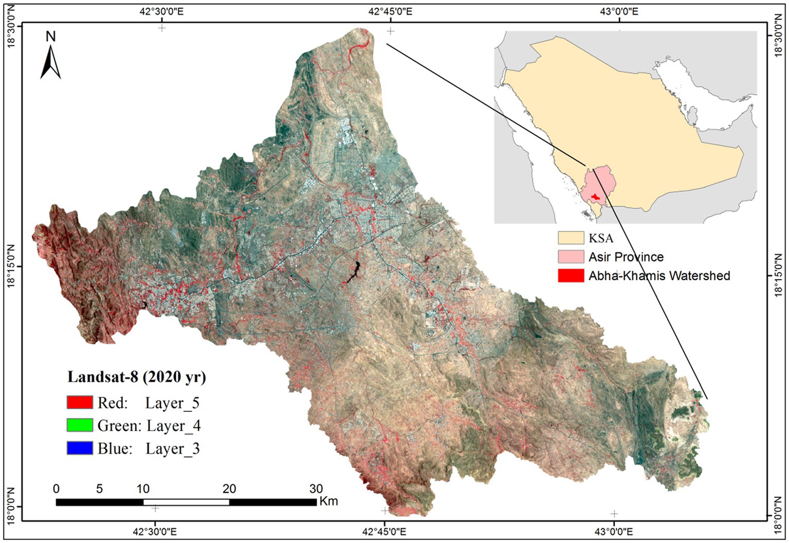
Figure 1. Location of the study area as Abha-Khamis watershed, Saudi Arabia.

2.2. Sampling of soils with laboratory analysis

Using a Global Positioning System (GPS) model GPS 38S, soil samples were gathered from the study region during dry weather conditions using a stratified technique, i.e., an area separated into areas with similar topography, soil moisture, and land cover. A total of one hundred thirty five (135) soil samples were taken from each site, with two replicates separated by 2–3 meters and 0–30 centimeters in depth. After air-drying soil samples at 102°C for 24 h in an oven, they were carefully homogenized, sieved through a 2-mm mesh, and then analyzed for their qualities, including soil texture and organic matter content, according to Carter’s standard process (1993). Using a muffle furnace at 350–600°C for 2 h, the organic matter content was determined. The precision of the measurements is specified to be 1.5% of the amount observed, with a detection limit of 0.02% (Hill and Schütt, 2000). Using the hydrometer method and Stokes’ law, the soil samples were analyzed for texture (Sheldrick and Wang, 1993).

2.3. Method for computing soil erodibility indices

In the present study, we have computed three conventional SEIs and proposed one PCA based SEI method for investigating the soil erodibility.

2.3.1. Computation of clay ratio

The clay ratio is an evaluation of the quantity of the binding agent clay that securely binds the soil particles, making it difficult for the particle to be detached by the external forces in the presence of a larger number of clay particles (Bouyoucos, 1935). Ten percent minimum clay content is required for any interpretation (Bryan, 1968). Soil erodibility decreases as CR rises. The computation of clay ratio Eq. 1 is mentioned below

$\begin{array}{ll}CR=\left(\%\mathit{sand}+\%\mathit{silt}\right)/\%\mathit{clay}& (1)\end{array}$

2.3.2. Computation of modified clay ratio

Correlation analyses between soil characteristics have shown that the modified clay ratio may be used as an alternative measure of soil erodibility, as reported by Mukhi (1988) and Tarafdar and Ray (2005). They found that in high-organic-content soil, MCR was a better explanation of erodibility than CR. It can be computed using Eq. 2:

$\begin{array}{ll}MCR=\left(\%\mathit{sand}+\%\mathit{silt}\right)/\left(\%\mathit{clay}+\%OM\right)& (2)\end{array}$

2.3.3. Computation of critical level of soil organic matter

An indication of how susceptible soil is to erosion is referred to as the critical level of soil organic matter (CLOM). CLOM, according to Pieri (2012), has an effect on soil structure, which provides resistance to erosion. In their research, if CLOM is 5% or below, soil structure is lost and erosion susceptibility is high, 5–7% is moderate, and >9% shows stable soil structure, enabling better erosion resistance. The following Eq. 3 was used to get an estimate for the Critical Soil Organic Matter:

$\begin{array}{ll}\mathit{CLOM}=\frac{OM}{\mathit{Clay}+\mathit{Silt}}& (3)\end{array}$

2.3.4. Computation of PCA based soil erodibility index

In the present study, we proposed a PCA-based soil erodibility index (PSEI) method for computing robust SEI, where different parameters can contribute. An indexing method was used to determine the SEI which has been shown to work well for small-scale applications, including on-filed studies (Andrews et al., 2002). A SEI is the result of three phases: (i) determination of the minimum dataset (MDS) of indicators with the best representation of the soil structure related to erosion; (ii) standardization of MDS indicators; and (iii) combining the scores of the indicators.

Principal component analysis (PCA) was used to refine indicators suitable for the MDS. PCA reduces dimensionality and minimizes information loss. This is done by constructing unrelated variables called principal components (PCs), which are arranged so that the first few retain most of the volatility of the original data. The 9 previously standardized soil chemical and physical variables were subjected to PCA analysis. Standardized variables contain unit variance, so the PCA variance is equal to the number of observed variables. An eigenvalue is the numerical representation of a PC’s proportional contribution to the total variance. Using the eigenvalue criterion one (Kaiser, 1960) and the Scree test, the number of components was reduced (Cattell, 1966). Any component with an eigenvalue greater than 1.00 should be retained. Due to the fact that each of the observed standardized variables contributes one unit of variance, a PC with an eigenvalue less than 1.00 can be said to represent less variation than a single standardized variable. The Scree test plots the eigenvalues of each PC in descending order, picking the PC’s up to the bend in the graph.

Component loading or variable weights under a PC have been used to reduce the number of variables. For each PC, we considered only those variables that were in the top 10% in terms of absolute component loading (Wander and Bollero, 1999). Correlation analysis was used to assess whether heavily weighted factors were redundant and could be reduced further. The MDS indicators were converted into unitless combinable values from 0 to 1 to account for their contribution to soil functions. Wymore (1993) provided an equation for constructing three scoring curves: higher is better, lower is better, and optimal (a bell-shaped curve). A thorough knowledge of the relationship between the indicator and the quality of the soil is necessary to determine which function accomplishes what, i.e., the best shape for each indication. More is better should be used when increasing the level of the indicator improves the quality of the soil. The indicators whose increment decreases the quality of the soil correspond to the curve less is better. The optimal curve ranks indicators having a positive relationship with soil quality up to an ideal threshold, above which the SQ decreases.

After determining the type of indicator curve, the baseline, thresholds, and slope of the scoring function should be defined to account for deviations in the expected ranges due to soil, climate, and crop. The literature review and researchers’ opinions were used to determine the function and critical limits of each indicator.

After obtaining the S values for all of the indicator parameters, the PCA statistics were used to weight each characteristic. Each PC was responsible for explaining a particular percentage (%) of the whole data set’s variance. Once S and W were determined, the PSEI for each location could be computed using Eq. (4). When the index score is higher, it indicates that the erodability of the soil is higher.

$\begin{array}{ll}\mathit{PSEI}={\displaystyle \sum }_{i=1}^{n}S{E}_j\times S& (4)\end{array}$

2.4. Application of statistical tests for finding out the differences among the soil erodibility indices

The pairwise t-test was used to compare the means of each SEI with every other index prepared in this study. A t-test is a statistical test that is used to determine if the means of two groups are significantly different from each other. The t-test calculates two outputs: the t-value and the value of p. The t-value measures the difference between the means of the two groups relative to the variance within the groups, while the value of p measures the probability of observing a t-value as extreme as the one calculated if the means of the two groups were actually equal. If the value of p is less than a pre-determined significance level (usually 0.05), it is concluded that there is a statistically significant difference between the two indices being compared. By using a pairwise t-test, we can identify which indices have significantly different means from each other and thus provide insights into the differences between the soil erodibility indices.

2.5. Application of artificial neural network to find out best SEI

Artificial Neural Networks (ANN) is a class of machine learning algorithms that are inspired by the structure and functioning of the human brain (Boger and Guterman, 1997). ANN models consist of layers of interconnected artificial neurons that process and transmit information. ANN has been widely used in the field of agriculture and soil science for various applications, including soil erosion prediction (Garg et al., 2022; Egbueri et al., 2023).

In this study, TensorFlow and Keras were used to implement an ANN regression model to predict the soil erodibility indices based on the given features. The four soil erodibility indices CR, MCR, CLOM, and PCA were considered as the target variables, and the other relevant soil properties were considered as features. The ANN regression model is trained using a large dataset of soil properties and particular SEI. The process is repeated for four times, because we have four target variables with the same model architecture. During the training process, the model learns to optimize the weights of its connections by minimizing the error between the predicted and actual values (Nouri et al., 2023). The model’s performance is evaluated using metrics such as Mean Squared Error (MSE), Root Mean Squared Error (RMSE), R-squared (R²), and Mean Absolute Error (MAE). The ANN model’s architecture consists of an input layer, two hidden layers, and an output layer. Each layer contains a set of neurons that perform a specific computation. The input layer receives the input features, and the output layer produces the predicted soil erodibility indices. The hidden layers perform intermediate computations between the input and output layers, and each neuron’s output is determined by an activation function. The activation function introduces non-linearity into the model and enables it to learn complex relationships between the input features and the target variables (Nouri et al., 2023).

The model’s performance can be improved by tuning its hyperparameters such as the number of hidden layers, number of neurons per layer, learning rate, batch size, and number of epochs. These hyperparameters are optimized using techniques such as Grid Search, Random Search, and Bayesian optimization. Once the model is trained and optimized, it can be used to predict the soil erodibility indices for new soil samples. The model’s prediction accuracy can be further improved by using a larger and more diverse dataset for training and by including additional relevant features.

2.6. Improving the soil erosion management decision making using ANN derived SHAP model

Shapley additive explanations is a popular model-agnostic interpretability technique used to explain the predictions of machine learning models, including ANN models (Wieland et al., 2021). The SHAP values are calculated for each input feature and indicate the contribution of each feature to the model’s output (Al-Najjar et al., 2022).

In this study, the SHAP values were derived from the ANN model to identify which input features are responsible for soil erosion and their impact on the soil erodibility indices. The SHAP values can be used to generate a summary plot that displays the feature importance rankings in descending order (Tang et al., 2022). This summary plot can be used for soil erosion management purposes to identify the most important features and develop effective strategies to manage soil erosion (Zhang et al., 2020; Mohammadifar et al., 2021). The SHAP values are calculated using game theory concepts and define the contribution of each feature by comparing the model’s predictions with and without that feature. The SHAP values are additive, meaning that the sum of the SHAP values for all features equals the difference between the model’s output and the baseline prediction (Tang et al., 2022). The summary plot generated from the SHAP values displays the most important features at the top of the plot, with the corresponding SHAP values indicating the feature’s impact on the soil erodibility indices. The summary plot can be used to identify the most important features and develop effective strategies to manage soil erosion. For example, if the summary plot shows that rainfall intensity is the most important feature contributing to soil erosion, then soil conservation strategies could focus on reducing runoff and increasing infiltration.

3. Results

3.1. Descriptive assessment and spatial mapping of soil parameters

To assess the impact of land management techniques on soil quality, it is essential to evaluate various physicochemical parameters of the soil, including sand, silt, clay, soil density, moisture content, porosity, and the status of soil organic matter. The results of the SEI are presented in Figure 2, which confirms that SOC, soil density, porosity, and soil particles exhibit significant differences in soil quality/physicochemical properties at the 95% level of statistical confidence (Figure 2). Without a correlation between soil physicochemical properties, identification of underlying factor patterns would not be possible (Brejda et al., 2000). However, the two-tailed correlation matrix for the soil properties in the samples retrieved from the study area showed several correlations among the variables, with significant relationships (p < 0.05) being identified among the maximum number of possible soil properties. This large amount of correlation indicates that they can be grouped into a homogeneous set of variables based on their correlation patterns. Thus, these variables can be used as indicators of soil quality in conjunction with the land use management categories identified in the study area. The correlation between soil properties and SEI suggests that soil quality increased as soil properties such as SOC, porosity, and moisture content increased.

FIGURE 2

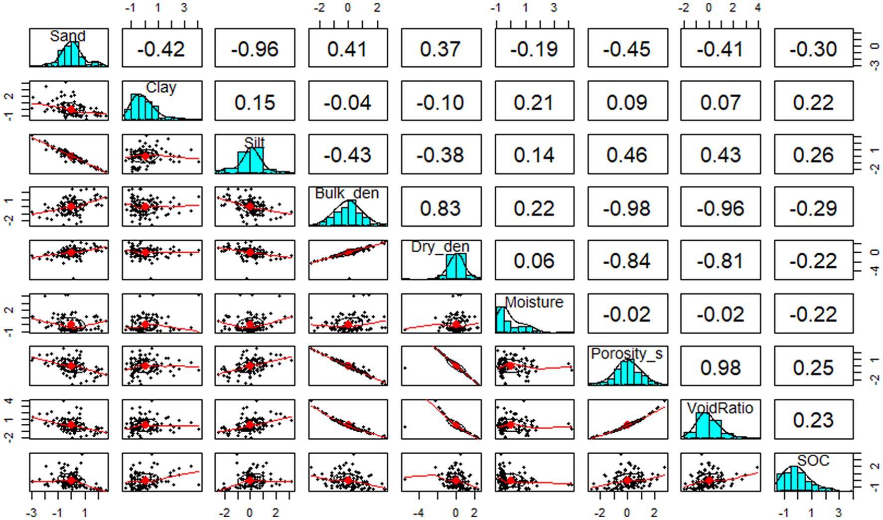
Figure 2. Relationship between different soil parameters using Pearson’s correlation coefficient technique.

Soil texture is a crucial characteristic that influences the infiltration rates of water from the soil surface (Figures 3A-I). Additionally, soil texture plays a significant role in the soil’s capacity to retain water and nutrients. The concentration of sand in the soil remained low in most of the study area, particularly in the northwestern site, while it increased in other areas of the study (Figures 3A,C). The northwestern site showed a high silt content that decreased in other regions of the study area. The textural classification of the northwestern area remained as sandy to silty loam texture. The distribution of clay concentration in the soil of the study area indicated a very low class distributed from the northeastern area to the southeastern area. A slightly higher level of clay content was observed in the northwestern part of the study area. The distribution of clay in soil samples suggested that the studied soils have low erodibility due to the cohesiveness of clay particles that form soil aggregates. This study revealed that clay had a negative correlation with soil erodibility (sand particles). The content of clay varied in the study area due to factors such as parent material, mineral characteristics, and weathering processes.

FIGURE 3

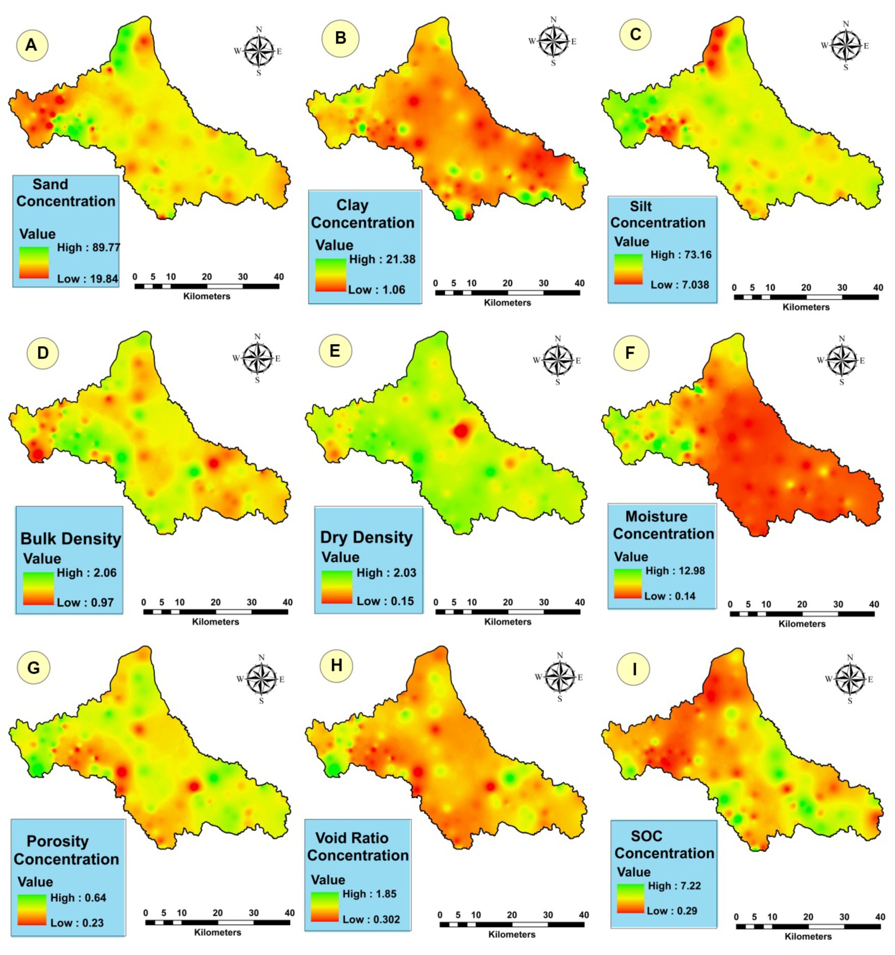
Figure 3. Spatial mapping of the concentration of different physical and chemical parameters, such as (A) sand, (B) clay, (C) silt, (D) bulk density, (E) dry density, (F) moisture, (G) porosity, (H) void ratio, (I) SOC.

The soil density was found to be high throughout the study area, as shown in Figures 3D,E. The decrease in soil attributes such as moisture content, porosity, and SOC content, along with an increase in bulk density, indicates that intensive tillage practices and lower plant productivity negatively affected soil compaction, microbial attributes, and soil aggregation. Annual tillage activities can disrupt soil aggregates and reduce physical protection of organic matter content, leading to lower SOC content and labile fractions in tilled soils compared to no-tilled soils (Green et al., 2007). The lower SOC content in cultivated soils can also have a negative impact on soil chemical, physical, and microbial properties (Ding et al., 2013; Zandi et al., 2017; Nabiollahi et al., 2018). Figure 3I shows that some areas have increased SOC content, which may be due to higher plant litter inputs and no-till practices during the restoration period, resulting in greater carbon inputs into the soil (Guo et al., 2017).

3.2. Modeling and proposing of SEIs

3.2.1. Analysis of the conventional SEIs

In this study, we investigated the soil erodibility condition of the study area using three conventional SEIs, namely CR, MCR, and CLOM (Figure 4). The CR values in the study area ranged from moderate to high, with lower values observed in the Western part of the area. However, since CR is a ratio between erosion-susceptible primary particles and clay, it cannot provide conclusive information on erosion proneness. To draw meaningful conclusions, it is recommended that the clay content in the cultivated soil be more than 10% (Bryan, 1968), which was the case for all the samples in the study area. However, due to the absence of any scale for erosion proneness, conclusive interpretation could not be drawn for the present study.

FIGURE 4

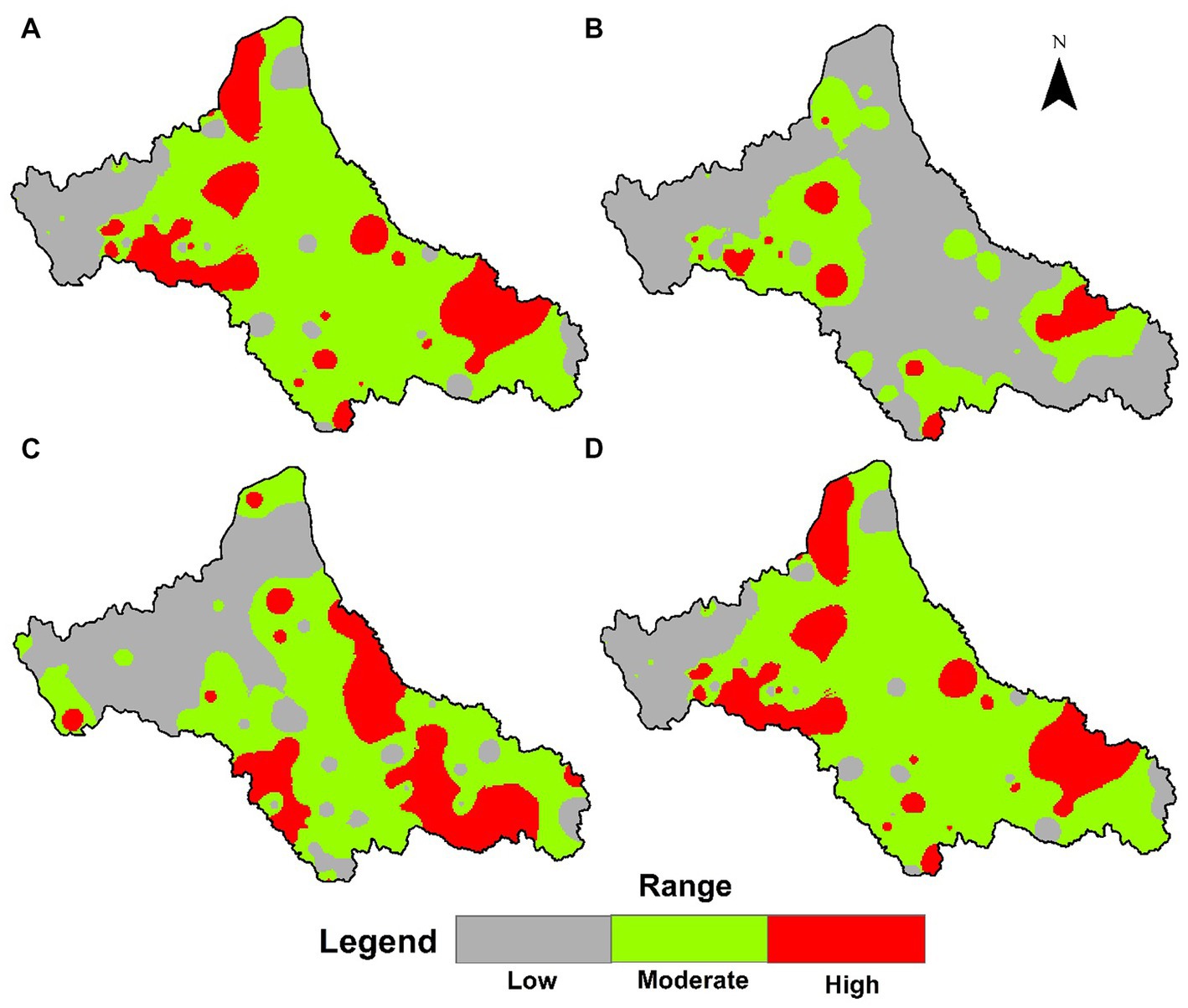
Figure 4. Computed soil erodibility indices, such as (A) CR, (B) MCR, (C) CLOM, and (D) PCA based SEI model for the Asir.

Other studies have suggested modified clay ratio (MCR) as another index for soil erosion due to the effects of wind, water, or other natural events (Mukhi, 1988; Tarafdar and Ray, 2005). In this study, the MCR values for the study area ranged from low to high, with most of the soil showing low MCR and a moderate trend of CR. Although the MCR values did not provide conclusive information on the erosion proneness of the soil according to land uses, the low average values indicated that the soils in the study area were not highly susceptible to erosion.

The results showed significant differences among CR and CLOM, with the contribution of 25–27% (Figure 4) accounting for >89% of the total variability. Moreover, significant correlations were observed between the CR and CLOM, with both contributing to the SEI of the study soils.

The CLOM values ranged from low to high, with 40% of the soil showing low CLOM, 40% showing moderate CLOM, and the remaining 20% showing high CLOM (Figure 4). These findings indicate that the soils in the study area had moderate to stable soil structure and offered resistance to erosion. Soil aggregate stability is related to soil organic matter, and the study area showed a range of soil organic carbon levels between 0.29 and 7.22% (Figure 3I). This is consistent with the CLOM findings, which revealed a positive correlation between soil stability and the amount of soil organic matter. However, it is important to note that these methods are entirely based on the developed equation.

3.2.2. Proposing PCA based SEI

In this study, instead of relying on equation-based SEIs, we employed a PCA-based weighting technique to develop a new SEI. The PCA analysis indicated that the first three principal components (PCs) accounted for over 10% of the total variance (Figure 5) and explained more than 68.4% of the variability among the various soil properties studied for SEI development. Bulk density is widely recognized as a reliable indicator of soil compaction, and the distribution map revealed a strong correlation between soil density and sand concentration, indicating that higher sand content in soils tends to result in higher bulk density due to the lower total pore space in sandy soils compared to silt or clay soils. Conversely, soils with finer textures, such as silt and clay loams, that display good structure tend to have higher pore space and lower bulk density compared to sandy soils. In our study, we also developed an index based on weights using the first PC of PCA. The weights were computed from the field-based data patterns obtained from Figure 5, rather than relying solely on equations. By using the weights generated from field-based data, we were able to compute erodibility in a more accurate and reliable way. The SEI developed using this approach revealed that 68% of the study area was covered by moderately erosion-prone areas, followed by 9 and 23% of the area being low and high erosion-prone, respectively (Figure 4D).

FIGURE 5

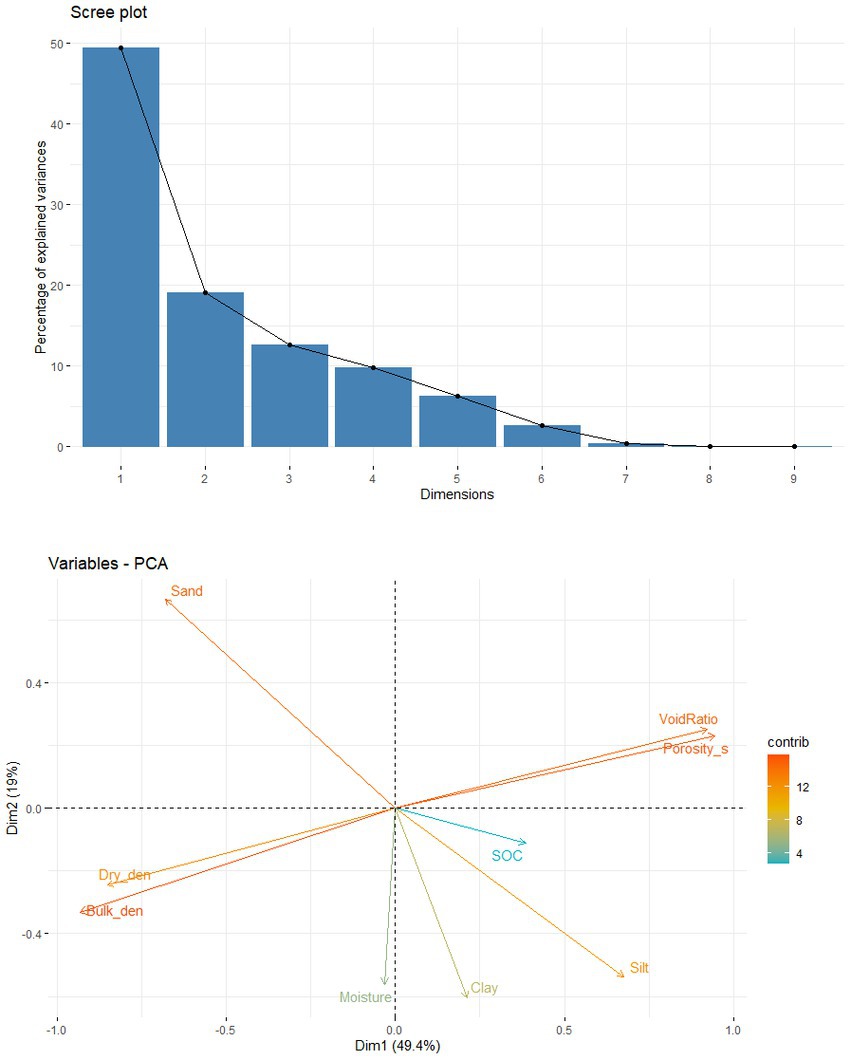
Figure 5. Application of PCA for feature selection.

3.3. Analysis of the difference among SEIs

In this study, the heatmap of correlation shows the correlations between the four soil erodibility indices - CR, MCR, CLOM, and PCA (Figure 6). The correlation coefficients show the strength and direction of the relationship between two variables. According to the heatmap, CR has a relatively strong positive correlation of 0.65 with PCA and an even stronger positive correlation of 0.75 with MCR. On the other hand, the correlation between CR and CLOM is weak with a coefficient of 0.036. This suggests that CR and MCR are likely to be highly related to each other, while CLOM may be less related to the other indices. CLOM has a weak negative correlation with PCA, with a coefficient of −0.047, indicating that these two indices are slightly negatively related to each other. Additionally, CLOM has a moderate negative correlation of −0.28 with MCR, suggesting that these two indices may be somewhat negatively related.

FIGURE 6

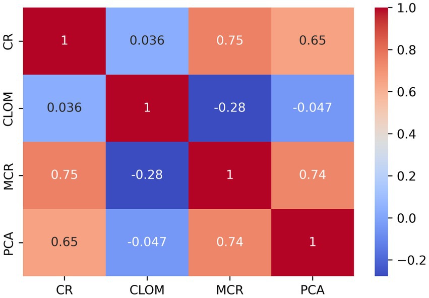
Figure 6. Correlation coefficient analysis among four SEIs for understanding the difference among them.

Finally, MCR has a strong positive correlation of 0.74 with PCA, indicating that these two indices are highly related to each other. This correlation is similar in strength to the correlation between CR and MCR, suggesting that both CR and MCR are highly related to PCA.

The results of the T-tests provide additional information on the differences between the four soil erodibility indices. A T-test is a statistical test used to determine if there is a significant difference between the means of two groups.

The T-test results show that there is a significant difference between the means of each pair of soil erodibility indices. The T-test for CR vs. CLOM shows a large t-value of 43.638 and a value of p of 0.00001, indicating a very significant difference between the means of these two indices. Similarly, the T-test for CR vs. MCR shows a large t-value of 33.643 and a value of p of 0.00001, indicating a very significant difference between the means of CR and MCR. The T-test for CR vs. PCA also shows a large t-value of 48.209 and a value of p of 0.00001, indicating a very significant difference between the means of CR and PCA. The T-test for CLOM vs. MCR shows a negative t-value of −11.072 and a value of p of 0.00001, indicating a significant difference between the means of these two indices, with CLOM having a lower mean than MCR. The T-test for CLOM vs. PCA shows a positive t-value of 14.615 and a value of p of 0.00001, indicating a significant difference between the means of these two indices, with PCA having a higher mean than CLOM. Finally, the T-test for MCR vs. PCA shows a positive t-value of 18.327 and a value of p of 0.00001, indicating a significant difference between the means of MCR and PCA, with PCA having a higher mean than MCR.

Based on the T-test results, CR is significantly different from CLOM, MCR, and PCA, while CLOM is significantly different from MCR and PCA, and MCR is significantly different from PCA.

3.4. Best SEI selection using ANN

We optimized the ANN model using grid search to find the best hyper-parameters. The best hyper-parameters are alpha = 0.17060, beta_1 = 0.0001, beta_2 = 0.0289, hidden_layer_sizes = 2, learning_rate_init = 0.0030, max_iter = 971, random_state = 42. These hyper-parameters are fixed for four models means CR with all parameters, MCR with all parameters, CLOM with all parameters, PCA with all parameters.

Figure 7 was used to illustrate the relationship between actual and predicted SEI values for the training and testing datasets for each of the four models. The R²values for CR were 0.93 and 0.82 for the training and testing datasets, respectively (Figures 7A,B). The R² values for MCR were 0.78 and 0.70 for the training and testing datasets, respectively (Figures 7C,D). The R² values for CLOM were 0.98 and 0.95 for the training and testing datasets, respectively (Figures 7E,F). The R² values for PCA were 0.73 and 0.60 for the training and testing datasets, respectively (Figures 7G,H).

FIGURE 7

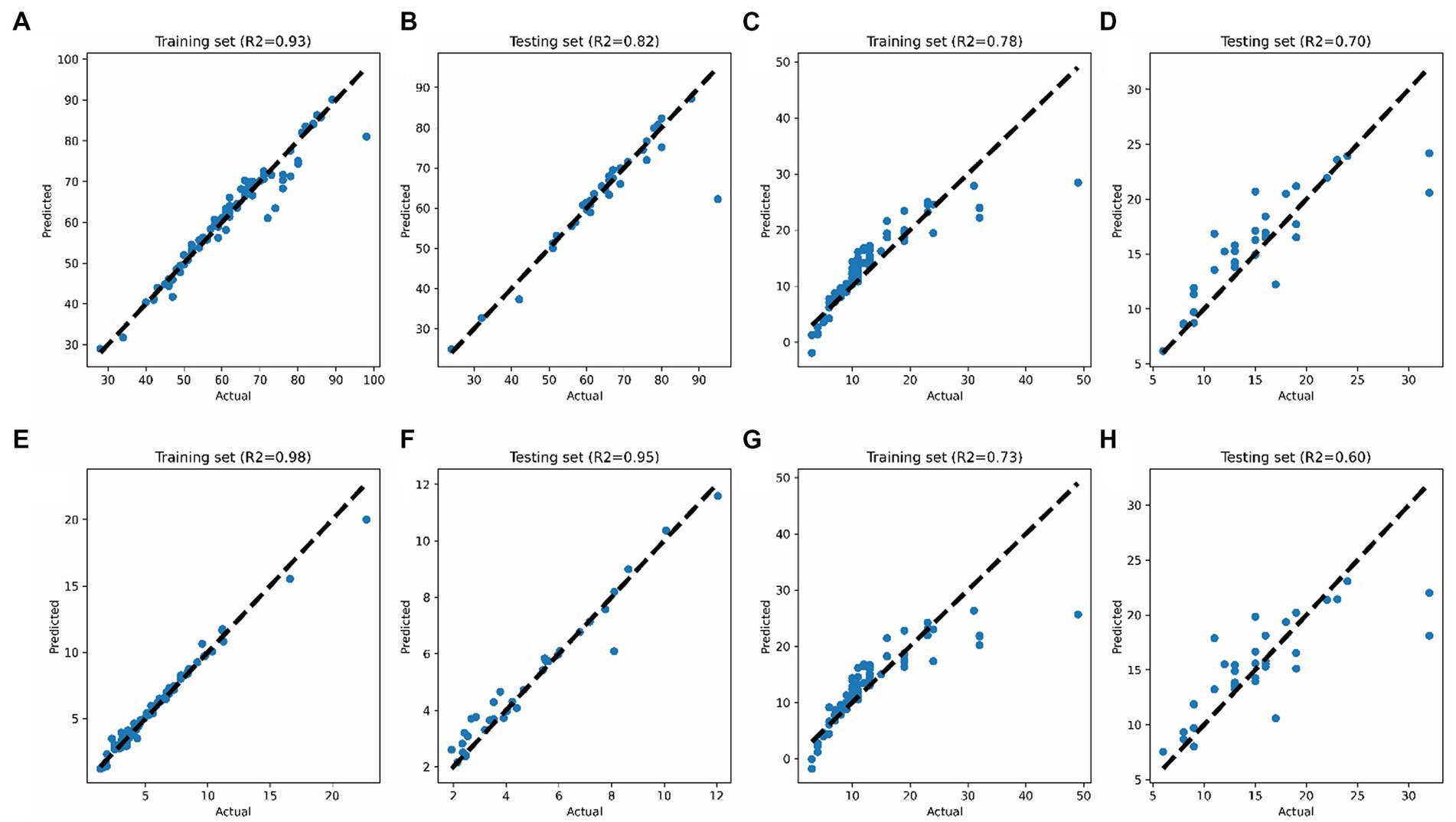
Figure 7. Selection of best SEI using optimized ANN model, for (A) training of CR, (B) testing of CR, (C) training of MCR, (D) testing of MCR, (E) training of CLOM, (F) testing of CLOM, (G) training of PCA, and (H) testing of PCA.

FIGURE 8

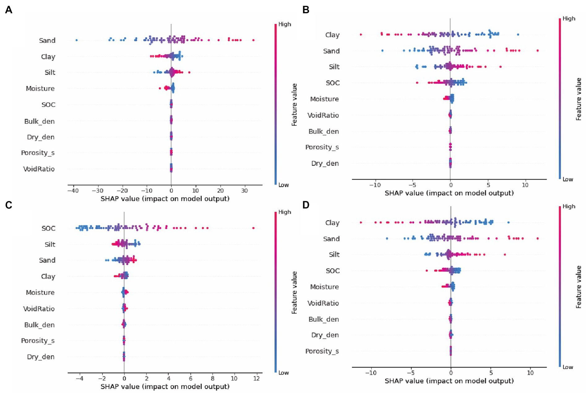
Figure 8. SHAP computation for (A) CR, (B) MCR, (C) CLOM, and (D) PCA based model.

The results of the ANN implementation show that CLOM is the best model for finding out soil erodibility based on the performance indices. This conclusion is based on the evaluation of the four models using R², RMSE, MSE, and MAE. The training and testing RMSE, MSE, and MAE values for CLOM were significantly lower than the values for the other models, indicating that the predictions made by the CLOM model are more accurate than those made by the other models.

The CLOM model had lower RMSE values than the other models, with values of 0.4781 for training and 0.5377 for testing. The superior performance of the CLOM model was further confirmed by the MSE and MAE values. Specifically, the MSE values for the CLOM model were 0.2286 for training and 0.2891 for testing, which were significantly lower than the values for the other models. Furthermore, the MAE values for the CLOM model were 0.2998 for training and 0.3489 for testing, which were again significantly lower than the values for the other models.

Therefore, it can be concluded that the CLOM model is the best model for finding out soil erodibility, and this information can be used for soil erosion management practices. The significantly lower values of performance indices indicate that the predictions made by the CLOM model are more accurate, which can help in developing more effective soil erosion management practices.

3.5. Improving decision making using SHAP

In this study, we used Artificial Neural Network (ANN) models to predict the SEI and calculated the SHAP values to identify the most influential variables for each of the four models, namely CR, MCR, CLOM, and PCA (Figure 8). The results showed that sand and silt were the most important variables for CR model, while clay, sand, silt, SOC, and moisture were highly influential for the MCR model. For the CLOM model, SOC, sand, moisture, and void ratio were found to be responsible for soil erosion, while silt and clay played a negative role. These findings have important implications for decision-making in soil erosion management. For example, the study suggests that sand and silt content are crucial factors that need to be monitored and managed to prevent soil erosion. This can be achieved through various management strategies, such as planting vegetation or using conservation tillage techniques. Additionally, the study highlights the importance of monitoring the anthropogenic activities that affect the soil properties, such as land use changes or tillage practices, which can have a significant impact on soil erosion.

4. Discussion

The study focused on the use of SEIs to effectively manage soil erosion, which is a significant environmental problem leading to soil degradation, loss of fertile land, and ecological imbalance. Several SEI models were compared using ANN model, and the best model was identified. To further improve soil erosion management, explainable artificial intelligence in the form of SHAP was introduced to quantify the influence of individual parameters in the model.

This study has provided insights into the effects of land use changes on soil recovery in native upland rangeland ecosystems. While soil quality index has been previously used to evaluate soil degradation and the effects of land conversion on soil quality (Li et al., 2013; Raiesi, 2017; Nabiollahi et al., 2018), this approach (use of AI for SEI assessment) has not been used to study the effects of cropland abandonment on soil recovery. The current study has used SEIs to determine soil physicochemical properties after a sequence of land use changes in native rangelands. The results indicated that the long-term activities for crop production on soil had a stronger influence on the quality of these soils, with lower values of SEI, moisture content, void ratio, and SOC observed in the study soils.

Different land use activities can negatively affect the soils, leading to decreases in SOM, soil moisture content, and soil structural stability, which can increase soil erodibility (Harris, 2010; Li et al., 2013; Raiesi and Riahi, 2014). The low values of SEI in soils suggest that the current cropland soils are in a degradation process, primarily due to the loss of soil structure, SOM, soil moisture content, and other physicochemical properties of soil (Raiesi and Salek-Gilani, 2020).

The observed deterioration of soil properties and function is likely due to low SOC input, soil moisture, and soil disturbance by human activities. Consistent with our observations, previous studies have reported soil quality degradation in cropland soils due to frequent tillage practices and little accumulation of plant residues in the surface soils (Raiesi, 2017; Zhang et al., 2019).

Our results showed that SEI values in the North-Western area were higher than those in other areas, which is likely due to the low SOC content at these sites (Figure 3I). In other areas of the study sites, SEI values were slightly higher, suggesting that soil quality can be restored when other physicochemical properties of soils are improved (Raiesi and Salek-Gilani, 2020). Therefore, the addition of SOC through improved cropping systems and the establishment and development of natural vegetation on eroded cropland soils in the study area can switch soil degradation to soil quality, except in the North-Western area.

The study findings indicate that ANN models can be highly accurate in predicting SEI, and the selection of the best model for predicting soil erodibility can be achieved by utilizing four indices, including CR, MCR, CLOM, and PCA. The results of the study showed that CLOM was the best model among the four indices, and the significant factors in predicting soil erodibility included SOC, silt, clay, sand, moisture, and void ratio.

The results of this study suggest that SOC and moisture content are critical variables for the CLOM model, indicating that management practices such as conservation tillage or adding organic matter to the soil can help to increase SOC content and improve soil moisture, thereby reducing soil erosion (Rojas et al., 2016; de Moraes Sa et al., 2018; Yang et al., 2019). Monitoring the void ratio can also help to prevent soil compaction and promote better soil structure. These findings have significant implications for soil erosion management, as soil erosion can lead to severe consequences such as soil degradation, loss of biodiversity, and reduced agricultural productivity.

To address this problem, management strategies should be proposed based on the significant factors identified in this study. Efforts can be made to increase the amount of clay and moisture in the soil, while reducing the amount of sand and silt, to reduce soil erosion. Additionally, anthropogenic activities should be monitored to determine their impact on soil erosion. Overall, the study demonstrates that the use of ANN models and SHAP values can provide valuable insights into the factors that contribute to soil erosion, and the findings can help policymakers and soil management practitioners in developing more effective management strategies to prevent soil erosion and preserve soil health.

This study also highlights the need for further research to assess the applicability of these findings across different soil types and geographic locations. It is important to note that while the study was conducted in a specific area, the results can be used as a foundation for future research in other locations.

The study may also provide valuable insights into the factors that influence soil erodibility, which can be used to develop effective soil erosion management strategies. By implementing these strategies, it is possible to minimize the adverse impact of soil erosion on the environment, agriculture, and society. Therefore, it is crucial for researchers to conduct further studies to validate and expand upon these findings, ultimately leading to better soil erosion management practices globally.

In inference, the study demonstrates the potential of using ANN models and SHAP values to predict soil erodibility with high accuracy. These findings provide significant implications for soil erosion management and suggest that promoting conservation practices and monitoring anthropogenic activities can help prevent soil erosion and preserve soil health. With further research, the findings can be applied globally, leading to more effective soil erosion management practices and a healthier environment.

5. Conclusion

This study provides a comprehensive assessment of different conventional SEI and proposed PCA based SEI with ANN model. Also, the most influencing parameters for SEI have been identified using XAI in the form of SHAP for explaining the interconnection between management practices, soil quality, and crop yields. Significant differences were observed among CR and CLOM with the contribution of 25–27% accounted for >89% of the total variability. The MCR for the 70% of the study area was observed as low, 20% moderate and 10% as high. CLOM for the study area ranged from low to high; where 40% of soil showed low CLOM, 40% of soil showed moderate and remaining 20% of soil fall under high CLOM. Based on the T-test results, CR is significantly different from CLOM, MCR, and PCA, while CLOM is significantly different from MCR and PCA, and MCR is significantly different from PCA. The ANN implementation demonstrated that the CLOM model had the highest accuracy for predicting soil erodibility, with SOC, sand, moisture, and void ratio being the most important variables. The SHAP analysis confirmed the importance of these variables for each of the four ANN models. These results highlight the importance of implementing effective soil erosion management strategies, especially in urban areas where erosion rates are highest. The results also suggest that monitoring and controlling anthropogenic activities that affect these variables, such as land use changes, construction, and irrigation practices, can help reduce soil erosion rates. Overall, these findings can inform policymakers and land managers on effective soil erosion management practices that can help protect soil health and ensure sustainable land use for future generations.

Despite the comprehensive approach used in this study to develop a standard SEI, there are limitations that should be considered. First, the study was conducted in a specific region, and the results may not be applicable to other regions with different soil types and environmental conditions. Second, the study only considered a limited number of soil attributes and did not incorporate biological indicators of soil quality, which are essential for the long-term sustainability of soil health. Finally, while the ANN models showed high accuracy in predicting soil erodibility, further research is needed to validate the results and assess their applicability to other regions.

Future research can build on the findings of this study to improve the accuracy and applicability of SEI models for different regions and soil types. Incorporating biological indicators of soil quality, such as microbial activity and biodiversity, can provide a more comprehensive understanding of soil health and sustainability. Additionally, the use of remote sensing techniques can help in the rapid assessment of soil erosion rates and inform soil erosion management strategies in real-time.

Data availability statement

The raw data supporting the conclusions of this article will be made available by the authors, without undue reservation.

Author contributions

JM, ST, and SA: conceptualization and formal analysis. JM and ST: data curation, methodology, software, and writing – original draft. SA: funding acquisition. JM: project administration, supervision, and validation. MA: resources and writing – review and editing. All authors contributed to the article and approved the submitted version.

Funding

Funding for this research was given under award numbers RGP2/185/43 by the Deanship of Scientific Research; King Khalid University, Ministry of Education, Kingdom of Saudi Arabia.

Acknowledgments

The authors extend their appreciation to the Deanship of Scientific Research at King Khalid University for funding this work through the Research Group under grant number RGP2/185/43. The authors are also thankful to the USGS Earth Explorer for making the LANDSAT data freely available.

Conflict of interest

The authors declare that the research was conducted in the absence of any commercial or financial relationships that could be construed as a potential conflict of interest.

Publisher’s note

All claims expressed in this article are solely those of the authors and do not necessarily represent those of their affiliated organizations, or those of the publisher, the editors and the reviewers. Any product that may be evaluated in this article, or claim that may be made by its manufacturer, is not guaranteed or endorsed by the publisher.

References

Al-Najjar, H. A., Pradhan, B., Beydoun, G., Sarkar, R., Park, H. J., and Alamri, A. (2022). A novel method using explainable artificial intelligence (XAI)-based Shapley additive explanations for spatial landslide prediction using time-series SAR dataset. Gondwana Res. doi: 10.1016/j.gr.2022.08.004

CrossRef Full Text | Google Scholar

Andrews, S. S., Karlen, D. L., and Mitchell, J. P. (2002). A comparison of soil quality indexing methods for vegetable production systems in Northern California. Agric. Ecosyst. Environ. 90, 25–45. doi: 10.1016/S0167-8809(01)00174-8

CrossRef Full Text | Google Scholar

Arrieta, A. B., Díaz-Rodríguez, N., Del Ser, J., Bennetot, A., Tabik, S., Barbado, A., et al. (2020). Explainable artificial intelligence (XAI): concepts, taxonomies, opportunities and challenges toward responsible AI. Inf. Fusion 58, 82–115. doi: 10.1016/j.inffus.2019.12.012

CrossRef Full Text | Google Scholar

Babur, E., Kara, O., Fathi, R. A., Susam, Y. E., Riaz, M., Arif, M., et al. (2021). Wattle fencing improved soil aggregate stability, organic carbon stocks and biochemical quality by restoring highly eroded Mountain region soil. J. Environ. Manag. 288:112489. doi: 10.1016/j.jenvman.2021.112489

PubMed Abstract | CrossRef Full Text | Google Scholar

Bhattacharyya, R., Ghosh, B. N., Mishra, P. K., Mandal, B., Rao, C. S., Sarkar, D., et al. (2015). Soil degradation in India: challenges and potential solutions. Sustainability 7, 3528–3570. doi: 10.3390/su7043528

PubMed Abstract | CrossRef Full Text | Google Scholar

Boger, Z., and Guterman, H., (1997) Knowledge extraction from artificial neural network models. In 1997 IEEE International Conference on Systems, Man, and Cybernetics. Computational Cybernetics and Simulation 4, 3030–3035). IEEE.

Google Scholar

Bora, M. J., Bordoloi, S., Pekkat, S., Garg, A., Sekharan, S., and Rakesh, R. R. (2022). Assessment of soil erosion models for predicting soil loss in cracked vegetated compacted surface layer. Acta Geophys. 1–15. doi: 10.1007/s11600-021-00698-z

CrossRef Full Text | Google Scholar

Bouyoucos, G. J. (1935). Clay ratio as a criterion of susceptibility of soils to erosion. J. Am. Soc. Agron. 27, 738–741.

Google Scholar

Brejda, J. J., Karlen, D. L., Smith, J. L., and Allan, D. L. (2000). Identification of regional soil quality factors and indicators II. Northern Mississippi Loess Hills and Palouse Prairie. Soil Sci. Soc. Am. J. 64, 2125–2135. doi: 10.2136/sssaj2000.6462125x

CrossRef Full Text | Google Scholar

Bryan, P. R. (1968). Measures of the degree of chemical weathering of rocks. J. Geol. 76, 518–527.

Google Scholar

Cattell, R. B. (1966). The Scree test for the number of factors. Multivar. Behav. Res. 1, 245–276. doi: 10.1207/s15327906mbr0102_10

PubMed Abstract | CrossRef Full Text | Google Scholar

Das, S., Deb, P., Bora, P. K., and Katre, P. (2020). Comparison of RUSLE and MMF soil loss models and evaluation of catchment scale best management practices for a mountainous watershed in India. Sustainability 13:232. doi: 10.3390/su13010232

CrossRef Full Text | Google Scholar

de Almeida Valente, F. D., de Castro, M. F., Lustosa Filho, J. F., de Carvalho Gomes, L., Neves, J. C. L., da Silva, I. R., et al. (2023). Native multispecies and fast-growing forest root biomass increase C and N stocks in a reclaimed bauxite mining area. Environ. Monit. Assess. 195:129. doi: 10.1007/s10661-022-10720-6

CrossRef Full Text | Google Scholar

de Moraes Sa, J. C., Potma Goncalves, D. R., Ferreira, L. A., Mishra, U., Inagaki, T. M., Ferreira Furlan, F. J., et al. (2018). Soil carbon fractions and biological activity based indices can be used to study the impact of land management and ecological successions. Ecol. Indic. 84, 96–105. doi: 10.1016/j.ecolind.2017.08.029

CrossRef Full Text | Google Scholar

Ding, F., YL, Y. L. H., Li, L. J., Li, A., Shi, S., Lian, P. Y., et al. (2013). Changes in soil organic carbon and total nitrogen stocks after conversion of meadow to cropland in Northeast China. Plant Soil 373, 659–672. doi: 10.1007/s11104-013-1827-5

CrossRef Full Text | Google Scholar

Dissanayake, D. M. S. L. B., Morimoto, T., and Ranagalage, M. (2019). Accessing the soil erosion rate based on RUSLE model for sustainable land use management: A case study of the Kotmale watershed, Sri Lanka. Model. Earth Syst. Environ. 5, 291–306. doi: 10.1007/s40808-018-0534-x

CrossRef Full Text | Google Scholar

Duarte, A. C., Ferreira, C., and Vitali, G. (2022). “Use of simulation models to aid soil and water conservation actions for sustainable agro-forested systems,” in Natural Resources Conservation and Advances for Sustainability. Elsevier, 389–412.

Google Scholar

Egbueri, J. C., Igwe, O., Omeka, M. E., and Agbasi, J. C. (2023). Development of MLR and variedly optimized ANN models for forecasting the detachability and liquefaction potential index of erodible soils. Geosyst. Geoenviron. 2:100104. doi: 10.1016/j.geogeo.2022.100104

CrossRef Full Text | Google Scholar

Esa, E., Assen, M., and Legass, A. (2018). Implications of land use/cover dynamics on soil erosion potential of agricultural watershed, northwestern highlands of Ethiopia. Environ. Syst. Res. 7, 1–14. doi: 10.1186/s40068-018-0122-0

CrossRef Full Text | Google Scholar

García, M. V., and Aznarte, J. L. (2020). Shapley additive explanations for NO2 forecasting. Eco. Inform. 56:101039. doi: 10.1016/j.ecoinf.2019.101039

CrossRef Full Text | Google Scholar

Garg, A., Wani, I., and Kushvaha, V. (2022). Application of artificial intelligence for predicting erosion of biochar amended soils. Sustainability 14:684. doi: 10.3390/su14020684

CrossRef Full Text | Google Scholar

Gilani, H., Ahmad, A., Younes, I., and Abbas, S. (2022). Impact assessment of land cover and land use changes on soil erosion changes (2005–2015) in Pakistan. Land Degrad. Dev. 33, 204–217. doi: 10.1002/ldr.4138

CrossRef Full Text | Google Scholar

Gong, C., Tan, Q., Liu, G., and Xu, M. (2022). Impacts of mixed forests on controlling soil erosion in China. Catena 213:106147. doi: 10.1016/j.catena.2022.106147

PubMed Abstract | CrossRef Full Text | Google Scholar

Green, V. S., Stott, D. E., Cruz, J. C., and Curi, N. (2007). Tillage impacts on soil biological activity and aggregation in a Brazilian Cerrado Oxisol. Soil Tillage Res. 92, 114–121. doi: 10.1016/j.still.2006.01.004

CrossRef Full Text | Google Scholar

Guo, D., Wang, J., Fu, H., Wen, H., and Luo, Y. (2017). Cropland has higher soil carbon residence time than grassland in the subsurface layer on the Loess Plateau, China. Soil Tillage Res. 174, 130–138. doi: 10.1016/j.still.2017.07.003

CrossRef Full Text | Google Scholar

Harris, R. B. (2010). Rangeland degradation on the Qinghai-Tibetan Plateau: A review of the evidence of its magnitude and causes. J. Arid Environ. 74, 1–12. doi: 10.1016/j.jaridenv.2009.06.014

CrossRef Full Text | Google Scholar

Hill, J., and Schütt, B. (2000). Mapping complex patterns of erosion and stability in dry Mediterranean ecosystems. Remote Sens. Environ. 74, 557–569. doi: 10.1016/S0034-4257(00)00146-2

CrossRef Full Text | Google Scholar

Jiang, X. J., Liu, W., Wu, J., Wang, P., Liu, C., and Yuan, Z. Q. (2017). Land degradation controlled and mitigated by rubber-based agroforestry systems through optimizing soil physical conditions and water supply mechanisms: a case study in Xishuangbanna. Land Degrad. Develop. 28, 2277–2289. doi: 10.1002/ldr.2757

CrossRef Full Text | Google Scholar

Kaiser, H. F. (1960). The application of electronic computers to factor analysis. Educ. Psychol. Meas. 20, 141–151. doi: 10.1177/001316446002000116

PubMed Abstract | CrossRef Full Text | Google Scholar

Kebede, Y. S., Endalamaw, N. T., Sinshaw, B. G., and Atinkut, H. B. (2021). Modeling soil erosion using RUSLE and GIS at watershed level in the Upper Beles, Ethiopia. Environ. Challenges 2:100009. doi: 10.1016/j.envc.2020.100009

CrossRef Full Text | Google Scholar

Khalil, U., and Aslam, B. (2022). Geospatial-based soil management analysis using novel technique for better soil conservation. Model. Earth Syst. Environ. 8, 259–275. doi: 10.1007/s40808-020-01078-0

CrossRef Full Text | Google Scholar

Kumar, H., and Pani, P. (2022). Soil erosion assessment in a part of gully affected Chambal region, Uttar Pradesh (India), using Morgan–Morgan–Finney model. Model. Earth Syst. Environ. 8, 5279–5288. doi: 10.1007/s40808-022-01375-w

CrossRef Full Text | Google Scholar

Li, X., Gao, J., Brierley, G., Qiao, Y., Zhang, J., and Yang, Y. (2013). Rangeland degradation on the Qinghai-Tibet Plateau: implications for rehabilitation. Land Degrad. Dev. 24, 72–80. doi: 10.1002/ldr.1108

CrossRef Full Text | Google Scholar

Mallick, J. (2016). Geospatial-based soil variability and hydrological zones of Abha semi-arid mountainous watershed, Saudi Arabia. Arab Jour Geosci 9:281. doi: 10.1007/s12517-015-2302-9

CrossRef Full Text | Google Scholar

McCool, D. K., Brown, L. C., Foster, G. R., Mutchler, C. K., and Meyer, L. D. (1987). Revised slope steepness factor for the Universal Soil Loss Equation. Transac ASAE 30, 1387–1396. doi: 10.13031/2013.30576

PubMed Abstract | CrossRef Full Text | Google Scholar

Meinen, B. U., and Robinson, D. T. (2021). Agricultural erosion modelling: Evaluating USLE and WEPP field-scale erosion estimates using UAV time-series data. Environ. Model Softw. 137:104962. doi: 10.1016/j.envsoft.2021.104962

CrossRef Full Text | Google Scholar

Millward, A., and Mersey, J. (1999). Adapting the RUSLE to Model Soil Erosion Potential in a Mountainous Tropical Watershed. Catena 38, 109–129. doi: 10.1016/S0341-8162(99)00067-3

CrossRef Full Text | Google Scholar

Mirzaee, S., and Ghorbani-Dashtaki, S. (2021). Calibrating the WEPP model to predict soil loss for some calcareous soils. Arab. J. Geosci. 14, 1–10. doi: 10.1007/s12517-021-08646-3

CrossRef Full Text | Google Scholar

Mohammadifar, A., Gholami, H., Comino, J. R., and Collins, A. L. (2021). Assessment of the interpretability of data mining for the spatial modelling of water erosion using game theory. Catena 200:105178. doi: 10.1016/j.catena.2021.105178

CrossRef Full Text | Google Scholar

Mukhi, A. K. (1988). Credibility of some vertisols. J. Indian Soc. Soil Sci. 36, 532–535.

Google Scholar

Nabiollahi, K., Golmohamadi, F., Taghizadeh-Mehrjardi, R., Kerry, R., and Davari, M. (2018). Assessing the effects of slope gradient and land use change on soil quality degradation through digital mapping of soil quality indices and soil loss rate. Geoderma 318, 16–28. doi: 10.1016/j.geoderma.2017.12.024

CrossRef Full Text | Google Scholar

Naseri, F., Azari, M., and Dastorani, M. T. (2021). Spatial optimization of soil and water conservation practices using coupled SWAT model and evolutionary algorithm. Int. Soil Water Conserv. Res. 9, 566–577. doi: 10.1016/j.iswcr.2021.04.002

CrossRef Full Text | Google Scholar

Nearing, M. A., Jetten, V., Baffaut, C., Cerdan, O., Couturier, A., Hernandez, M., et al. (2005). Modeling response of soil erosion and runoff to changes in precipitation and cover. Catena 61, 131–154. doi: 10.1016/j.catena.2005.03.007

PubMed Abstract | CrossRef Full Text | Google Scholar

Nouri, A., Esfandiari, M., Eftekhari, K., Torkashvand, A. M., and Ahmadi, A. (2023). Development support vector machine, artificial neural network and artificial neural network–genetic algorithm hybrid models for estimating erodible fraction of soil to wind erosion. Int. J. River Basin Manage. 1–10. doi: 10.1080/15715124.2022.2153856

CrossRef Full Text | Google Scholar

Nyakatawa, E. Z., Reddy, K. C., and Lemunyon, J. L. (2001). Predicting soil erosion in conservation tillage cotton production systems using the revised universal soil loss equation (RUSLE). Soil Till. Res. 57, 213–224. doi: 10.1016/S0167-1987(00)00178-1

CrossRef Full Text | Google Scholar

Olaniya, M., Bora, P. K., Das, S., and Chanu, P. H. (2020). Soil erodibility indices under different land uses in Ri-Bhoi district of Meghalaya (India). Sci. Rep. 10, 1–13. doi: 10.1038/s41598-020-72070-y

CrossRef Full Text | Google Scholar

Pal, S. (2016). Impact of Massanjore dam on hydro-geomorphological modification of Mayurakshi river, Eastern India. Environ. Dev. Sustain. 18, 921–944. doi: 10.1007/s10668-015-9679-1

CrossRef Full Text | Google Scholar

Pal, S., Paul, S., and Debanshi, S. (2022). Identifying sensitivity of factor cluster based gully erosion susceptibility models. Environ. Sci. Pollut. Res. 29, 90964–90983. doi: 10.1007/s11356-022-22063-3

PubMed Abstract | CrossRef Full Text | Google Scholar

Pandey, S., Kumar, P., Zlatic, M., Nautiyal, R., and Panwar, V. P. (2021). Recent advances in assessment of soil erosion vulnerability in a watershed. Int. Soil Water Conserv. Res. 9, 305–318. doi: 10.1016/j.iswcr.2021.03.001

CrossRef Full Text | Google Scholar

Pieri, C. J. (2012). Fertility of soils: A future for farming in the West African savannah, vol. 10. Springer-Verlag, Berlin: Springer Science & Business Media.

Google Scholar

Raiesi, F. (2017). A minimum data set and soil quality index to quantify the effect of land use conversion on soil quality and degradation in native rangelands of upland arid and semiarid regions. Ecol. Indic. 75, 307–320. doi: 10.1016/j.ecolind.2016.12.049

CrossRef Full Text | Google Scholar

Raiesi, F., and Riahi, M. (2014). The influence of grazing exclosure on soil C stocks and dynamics, and ecological indicators in upland arid and semi-arid rangelands. Ecol. Indic. 41, 145–154. doi: 10.1016/j.ecolind.2014.01.040

CrossRef Full Text | Google Scholar

Raiesi, F, and Salek-Gilani, S., (2020). Development of a soil quality index for characterizing effects of land-use changes on degradation and ecological restoration of rangeland soils in a semi-arid ecosystem. Land Degrad. Dev. 31, 1533–1544. doi: 10.1002/ldr.3553

CrossRef Full Text | Google Scholar

Raza, A., Ahrends, H., Habib-Ur-Rahman, M., and Gaiser, T. (2021). Modeling approaches to assess soil erosion by water at the field scale with special emphasis on heterogeneity of soils and crops. Land 10:422. doi: 10.3390/land10040422

CrossRef Full Text | Google Scholar

Rieke, E. L., Bagnall, D. K., Morgan, C. L., Flynn, K. D., Howe, J. A., Greub, K. L., et al. (2022). Evaluation of aggregate stability methods for soil health. Geoderma 428:116156. doi: 10.1016/j.geoderma.2022.116156

PubMed Abstract | CrossRef Full Text | Google Scholar

Rojas, J. M., Prause, J., Sanzano, G. A., Arce, O. E. A., and Sánchez, M. C. (2016). Soil quality indicators selection by mixed models and multivariate techniques in deforested areas for agricultural use in NW of Chaco, Argentina. Soil Tillage Res. 155, 250–262. doi: 10.1016/j.still.2015.08.010

CrossRef Full Text | Google Scholar

Saha, S., Sarkar, D., and Mondal, P. (2022). Assessing and mapping soil erosion risk zone in Ratlam District, Central India. Reg. Sustain. 3, 373–390. doi: 10.1016/j.regsus.2022.11.005

CrossRef Full Text | Google Scholar

Senanayake, S., and Pradhan, B. (2022). Predicting soil erosion susceptibility associated with climate change scenarios in the Central Highlands of Sri Lanka. J. Environ. Manag. 308:114589. doi: 10.1016/j.jenvman.2022.114589

PubMed Abstract | CrossRef Full Text | Google Scholar

Sheldrick, B. H., and Wang, C. (1993). “Particle Size Analysis” in Soil sampling and methods of analysis. ed. M. R. Carter (Boca Raton: Lewis Publishers), 499–517.

Google Scholar

Shi, P., Li, P., Li, Z., Sun, J., Wang, D., and Min, Z. (2022). Effects of grass vegetation coverage and position on runoff and sediment yields on the slope of Loess Plateau. Agric Water Manag 259:107231. doi: 10.1016/j.agwat.2021.107231

CrossRef Full Text | Google Scholar

Shrestha, N. K., Rudra, R. P., Daggupati, P., Goel, P. K., and Shukla, R. (2021). A comparative evaluation of the continuous and event-based modelling approaches for identifying critical source areas for sediment and phosphorus losses. J. Environ. Manag. 277:111427. doi: 10.1016/j.jenvman.2020.111427

PubMed Abstract | CrossRef Full Text | Google Scholar

Stagnari, F., Ramazzotti, S., and Pisante, M. (2010). “Conservation agriculture: a different approach for crop production through sustainable soil and water management: a review” in Organic farming, pest control and remediation of soil pollutants. ed. E. Lichtfouse (Dordrecht: Springer), 55–83.

Google Scholar

Tang, Y., Duan, A., Xiao, C., and Xin, Y. (2022). The prediction of the Tibetan Plateau thermal condition with machine learning and Shapley additive explanation. Remote Sens. 14:4169. doi: 10.3390/rs14174169

CrossRef Full Text | Google Scholar

Tarafdar, P. K., and Ray, R. (2005). Effect of trees on improvement of physical environment and fertility in soils of West Bengal. Bull. Nat. Inst. Ecol. 16, 129–136.

Google Scholar

Telak, L. J., Dugan, I., and Bogunovic, I. (2021). Soil management and slope impacts on soil properties, hydrological response, and erosion in hazelnut orchard. Soil Syst. 5:5. doi: 10.3390/soilsystems5010005

CrossRef Full Text | Google Scholar

Tesfahunegn, G. B., Ayuk, E. T., and Adiku, S. G. K. (2021). Farmers’ perception on soil erosion in Ghana: Implication for developing sustainable soil management strategy. PLoS One 16:e0242444. doi: 10.1371/journal.pone.0242444

PubMed Abstract | CrossRef Full Text | Google Scholar

Toy, T. J., Foster, G. R., and Renard, K. G. (1999). RUSLE for mining, construction and reclamation lands. J. Soil Water Conserv. 54, 462–467.

Google Scholar

Tsesmelis, D. E., Karavitis, C. A., Kalogeropoulos, K., Zervas, E., Vasilakou, C. G., Skondras, N. A., et al. (2022). Evaluating the degradation of natural resources in the Mediterranean environment using the water and land resources degradation index, the case of Crete Island. Atmos. 13:135. doi: 10.3390/atmos13010135

CrossRef Full Text | Google Scholar

Vilone, G., and Longo, L. (2021). Notions of explainability and evaluation approaches for explainable artificial intelligence. Inform. Fus. 76, 89–106. doi: 10.1016/j.inffus.2021.05.009

PubMed Abstract | CrossRef Full Text | Google Scholar

Vincent, P. Saudi Arabia: an environmental overview (2008). CRC Press. Available at: https://www.routledge.com/Saudi-Arabia-An-Environmental-Overview/Vincent/p/book/9780367387815

Google Scholar

Vitali, F., Mandalakis, M., Chatzinikolaou, E., Dailianis, T., Senatore, G., Casalone, E., et al. (2019). Benthic prokaryotic community response to polycyclic aromatic hydrocarbon chronic exposure: Importance of emission sources in Mediterranean ports. Front. Mar. Sci. 6:590. doi: 10.3389/fmars.2019.00590

CrossRef Full Text | Google Scholar

Wander, M. M., and Bollero, G. A. (1999). Soil quality assessment of tillage impacts in Illinois. Soil Sci. Soc. Am. J. 63, 961–971. doi: 10.2136/sssaj1999.634961x

CrossRef Full Text | Google Scholar

Wassie, S. B. (2020). Natural resource degradation tendencies in Ethiopia: a review. Environ. Syst. Res. 9, 1–29. doi: 10.1186/s40068-020-00194-1

CrossRef Full Text | Google Scholar

Wieland, R., Lakes, T., and Nendel, C. (2021). Using Shapley additive explanations to interpret extreme gradient boosting predictions of grassland degradation in Xilingol. Geosci. Model Dev. 14, 1493–1510. doi: 10.5194/gmd-14-1493-2021

CrossRef Full Text | Google Scholar

Wymore, A.W. (1993) Model-based systems engineering. 1st, CRC Press, Boca Raton.

Google Scholar

Yang, Y., Tilman, D., Furey, G., and Lehman, C. (2019). Soil carbon sequestration accelerated by restoration of grassland biodiversity. Nat. Commun. 10:718. doi: 10.1038/s41467-019-08636-w

CrossRef Full Text | Google Scholar

Zandi, L., Erfanzadeh, R., and Jafari, H. (2017). Rangeland use change to agriculture has different effects on soil organic matter fractions depending on the type of cultivation. Land Degrad. Dev. 28, 175–180. doi: 10.1002/ldr.2589

CrossRef Full Text | Google Scholar

Zhang, Y., Xu, X., Li, Z., Liu, M., Xu, C., Zhang, R., et al. (2019). Effects of vegetation restoration on soil quality in degraded karst landscapes of southwest China. Sci. Total Environ. 650, 2657–2665. doi: 10.1016/j.scitotenv.2018.09.372

PubMed Abstract | CrossRef Full Text | Google Scholar

Zhang, K., Xu, P., and Zhang, J. (2020). “Explainable AI in deep reinforcement learning models: A shap method applied in power system emergency control” in In 2020 IEEE 4th Conference on Energy Internet and Energy System Integration (EI2) ( IEEE), 711–716.

Google Scholar

Zhang, X., Yu, G. Q., Li, Z. B., and Li, P. (2014). Experimental study on slope runoff, erosion and sediment under different vegetation types. Water Resour. Manag. 28, 2415–2433. doi: 10.1007/s11269-014-0603-5

CrossRef Full Text | Google Scholar

Zuo, F. L., Li, X. Y., Yang, X. F., Wang, Y., Ma, Y. J., Huang, Y. H., et al. (2020). Soil particle-size distribution and aggregate stability of new reconstructed purple soil affected by soil erosion in overland flow. J. Soils Sediments 20, 272–283. doi: 10.1007/s11368-019-02408-1

CrossRef Full Text | Google Scholar