Integrating machine learning and species distribution models for predicting the potential hazard areas of Marmota baibacina in Xinjiang, China

Introduction: Under global climate change and intensified human activities, species distributions are undergoing significant shifts. Marmota baibacina, a representative keystone species among Central Asian high-altitude species, exacerbates vegetation degradation and soil erosion through herbivory and burrowing activities. As the primary reservoir of Yersinia pestis, it poses a significant public health threat.

Methods: This study integrated five machine learning models (XGBoost, RF, SVM, LogBoost) and the MaxEnt model to predict the current (1970–2000) and future (2041–2100) distribution of Marmota baibacina under three climate scenarios (SSP126, SSP370, SSP585), utilizing 111 occurrence records and 29 environmental variables spanning climatic, topographic, edaphic, and vegetation dimensions.

Results: The results indicated that (1) All five models demonstrated high predictive accuracy with AUC values exceeding 0.9. After screening 29 environmental variables, machine learning models identified 10 key variables with high feature importance, while MaxEnt selected 16 environmental variables; (2) Dominant drivers revealed that Bio18 (warmest quarter precipitation), Bio2 (diurnal temperature range), Bio11 (coldest quarter temperature), and Bio15 (precipitation seasonality) collectively contributed >70% to machine learning models, whereas MaxEnt prioritized slope, NDVI, and Bio18; (3) Under current climatic conditions, the potential suitable habitats of Marmota baibacina in Xinjiang are primarily concentrated in the central Tianshan Mountains, with core distribution centers in Bayingolin Mongolian Autonomous Prefecture (Hejing County), Ili Kazakh Autonomous Prefecture, and the western part of Bortala Mongolian Autonomous Prefecture, The total suitable habitat area estimated by the five models ranged from 2.75 × 10⁴ km² to 13.59 × 10⁴ km² under the current climate; (4) Future projections under all scenarios indicated an overall decreasing trend in suitable habitat area, with habitat contraction particularly pronounced in the southern Tianshan under SSP585.

Discussion: Such distributional shifts may intensify competition between marmots and livestock, accelerate alpine meadow degradation, and elevate zoonotic plague transmission risks due to population aggregation. This study provides critical insights for balancing alpine ecosystem conservation and plague prevention strategies, offering actionable guidance for safeguarding ecological security and public health in Xinjiang’s ethnically diverse pastoral regions.

1 Introduction

Plague is a serious infectious and zoonotic disease whose primary host is rodents (Eisen et al., 2007; Stenseth et al., 2008). It has caused at least three large-scale epidemics (Stenseth et al., 2008). China is the largest and most extensive source of plague, and rodents are widely distributed across mountains, deserts, forests, and steppe (Addink et al., 2010), and most of them live in subterranean burrowing systems, which cause massive soil erosion and lead to degradation of ecosystems (Linné Kausrud et al., 2007; Addink et al., 2010; Prakash and Ghosh, 2012). Under global warming and intensified anthropogenic activities, shifts in Marmota baibacina’s habitat range and population dynamics may further threaten ecological balance and pastoral livelihoods. Therefore, accurately predicting its potential distribution and responses to climate change is crucial for balancing alpine ecosystem conservation and plague prevention in Xinjiang.

The Marmota baibacina is a representative keystone species among Central Asian high-altitude species. This large, social rodent primarily inhabits alpine meadows and steppes at elevations between 2,500 and 4,000 meters, where it constructs complex burrow systems (Koshkina et al., 2020). Its foraging and extensive burrowing activities significantly influence soil properties, hydrology, and plant community structure, classifying it as an ecosystem engineer (Addink et al., 2010). Beyond its ecological role, Marmota baibacina is the primary natural reservoir of Yersinia pestis, the bacterium responsible for plague, posing a substantial zoonotic threat to human populations (Davis et al., 2004). While not currently assessed on the IUCN Red List, its populations face growing pressures from climate change and anthropogenic activities. Its conservation status is intrinsically linked to its role as a disease reservoir, often leading to population control measures that may disrupt its ecological function. The primary threats to Marmota baibacina include climate-driven habitat shifts, which may alter the availability of its preferred mesic environments, and intensified competition with livestock for forage in degraded grasslands (Wang et al., 2024). Understanding its habitat requirements and distribution is therefore critical not only for biodiversity conservation but also for public health planning.

Xinjiang’s steppe covers an area of approximately 513,000 square kilometers, accounting for 30% of the total area of the region (An et al., 2023). Xinjiang’s grasslands are not only a critical component of Central Asian alpine ecosystems but also the cornerstone of livelihoods for local ethnic minorities, particularly Kazakh and Mongolian herders who rely heavily on livestock grazing. The degradation of grasslands caused by marmot burrowing and foraging directly threatens the sustainability of mutton and beef production, which are primary protein sources for these communities. Given the dual role of Marmota baibacina as an ecosystem engineer and a zoonotic reservoir, its population dynamics under climate change could exacerbate both ecological and socio-economic vulnerabilities in this ethnically diverse region. Marmota baibacina’s burrowing and foraging behaviors cause steppe degradation and soil erosion, and competition with livestock exacerbates this degradation (Davis et al., 2004; Addink et al., 2010). Furthermore, Marmota baibacina is a primary host for the plague bacterium, transmitting the disease to humans and other animals through fleas, posing a severe public health threat (Davis et al., 2004; Jäkel et al., 2016). With the intensification of climate change, Marmota baibacina’s habitat range and behaviors may change, leading to even greater impacts on ecosystems and human life (Koshkina et al., 2020). Therefore, studying the potential suitable habitat of Marmota baibacina under future climate scenarios will help to assess the effects of climate change on steppe ecological balance and provides scientific evidence for plague prevention.

Species distribution models (SDMs) serve as core tools for analyzing species-environment relationships and projecting habitat suitability (Yang et al., 2023; Zhao et al., 2023). Currently, increasing researches use SDMs to predict species distribution dynamics (Liu et al., 2023; Mo et al., 2023). SDMs utilize species occurrence data and predictor variables to model potential species distributions under changing climatic conditions (Jia et al., 2017; Zhang et al., 2023). With the development of computer technology and ecological modeling methods, multiple SDMs have been developed and applied to different research scenarios, such as Extreme Gradient Boosting (XGBoost), Random Forest (RF), Support Vector Machine (SVM), Logistic Boosting (LogBoost), and Maximum Entropy Model (MaxEnt). Depending on the data requirements for species distribution, models can be divided into two categories: profile techniques (e.g., BIOCLIM, MaxEnt, and GARP) requiring only species presence data; and group discrimination techniques (e.g., RF, SVM, ANN, and GBM) needing presence-absence data. Since the advent of R language, most algorithms used for species distribution analysis and prediction can run on the same data platform, making R the most commonly used modeling environment in species distribution modeling (Guisan et al., 2017). For example, Li et al. (2017) and Yang et al. (2015) used RF and SVM methods to establish fish egg distribution and prediction models, comparing them with traditional methods, and found that machine learning models outperformed others. Peters et al. (2007) used RF and multiple logistic regression models to predict vegetation species distribution in the Belgian valley and found that RF outperformed other models in terms of accuracy. Luo et al. (2017) used giant panda data to evaluate the performance of Biomod and MaxEnt distribution predictions, showing that Biomod performed better when distribution points were sparse. Zhai and Li (2012) used nine models in Biomod to simulate the suitable habitats of the crested ibis from 1950 to 2000 and predict its potential habitat range in 2020, 2050, and 2080. Zhang et al. (2011) compared random forests, generalized boosting methods, Neural Ensembles, generalized linear models, generalized additive models, and classification regression trees. They simulated and analyzed the suitable habitat of Masson pine under future climate scenarios, with RF performing the best. An et al. (2023) analyzed the impact of future climate change on the suitable habitat area and distribution pattern of Eolagurus luteus in Xinjiang, finding that its habitat area continued to decrease. Moreover, the MaxEnt model has been used to predict suitable habitats for plant species such as Parnassia wightiana (Dai et al., 2022), Jatropha curcas (Liu and Mai, 2022), and Polygonatum kingianum (Guo et al., 2023), achieving good results. These studies not only predicted the effects of future climate change on species’ suitable habitats but also explored the role of historical climate change in species distribution, further deepening the understanding of species’ mechanisms for responding to climate change. Reliable species absence data are usually unavailable; thus, background or pseudo-absence points are typically used instead. Related research has shown that models based on species presence/absence data typically outperform those based on species presence data alone (Liu et al., 2013). Currently, species distribution prediction models are widely applied in biogeography, and the choice of model can significantly influence the prediction results. MaxEnt is widely recognized for its robustness in handling presence-only data, which is particularly valuable when reliable absence data of species are scarce (Phillips et al., 2006). This advantage makes it suitable for studies on Marmota baibacina, as obtaining comprehensive absence records in the vast alpine regions of Xinjiang is logistically challenging. In contrast, the four machine learning models (XGBoost, RF, SVM, LogBoost) require presence-absence data and excel at capturing complex nonlinear relationships between species and environmental variables (Elith et al., 2008). By integrating MaxEnt with these machine learning models, we can not only leverage the strengths of each model—such as MaxEnt’s adaptability to limited data and RF’s ability to handle high-dimensional variables—but also conduct cross-validation to reduce prediction biases, thereby improving the reliability of habitat suitability assessments for Marmota baibacina.

Current research on Marmota baibacina’s habitat ecology remains insufficient, particularly regarding its dual ecological roles as both an ecosystem engineer through burrowing activities that exacerbate steppe degradation and a zoonotic reservoir for plague transmission. To address these knowledge gaps, this study employs an integrated modeling approach, utilizing comprehensive occurrence data from Xinjiang and 29 bioclimatic, topographic, and environmental variables. Through the R software platform, we implemented five distinct species distribution models (XGBoost, RF, SVM, LogBoost, and MaxEnt) to predict current and future habitat suitability across the Tianshan Mountains’ altitudinal gradient under multiple climate scenarios (Guisan et al., 2017; Zhao et al., 2023). The study aims to: (1) identify and quantify key environmental determinants of Marmota baibacina distribution, establishing optimal ranges for critical variables; (2) project spatiotemporal patterns of habitat suitability shifts under climate change scenarios, providing evidence-based insights for plague prevention strategies in Xinjiang; (3) conduct comparative model performance evaluations to determine the most reliable predictive framework for alpine species distribution modeling.

2 Materials and methods

2.1 Study area

The study area is located on the northern and southern of the Tianshan Mountain range in Xinjiang, China, covering the central section of the Tianshan Mountain and the surrounding regions on both sides. This area is a key habitat for Marmota baibacina (Figure 1). The Tianshan Mountain range runs through the central part of Xinjiang, dividing the study area into northern and southern regions, forming an ecological transition zone with distinct dry and wet conditions (Wang et al., 2021). The northern lies at the southern edge of the Tianshan Mountain and the Junggar Basin. The climate is temperate and humid, with high annual precipitation (200–800 mm). Forests, steppe, and alpine meadows are mainly distributed here, making it a region rich in water resources and biodiversity (Zhang et al., 2024). Areas such as the Ili River Valley and the Bortala River Valley are known as the “Jiangnan of the North,” with favorable natural conditions. The southern of the Tianshan Mountain is characterized by a typical arid continental climate, with low annual precipitation, dominated by deserts, gobi, and oasis. The northern of the Tianshan Mountains includes administrative regions such as Ili Kazakh Autonomous Prefecture, Bortala Mongolian Autonomous Prefecture, Urumqi, Changji Hui Autonomous Prefecture, and Turpan, which are economically developed and are key agricultural, pastoral, and industrial areas in Xinjiang (Fang et al., 2024). The southern of the Tianshan Mountains includes parts of Bayingolin Mongolian Autonomous Prefecture and Aksu Prefecture, with an economy based on oasis agriculture and resource development, with Korla City as the core city on the southern. Overall, the northern and southern of the Tianshan Mountains have significant differences in natural geography and ecological environments, making them important regions for studying climate change, biodiversity conservation, and ecosystem services (Wang et al., 2024). Marmota baibacina is widely distributed in the alpine meadows, steppe, and surrounding mountainous areas of the Tianshan Mountains, primarily inhabiting the high-altitude regions between 2,500 and 4,000 meters above sea level (Sun et al., 2018). It relies on the unique ecological and climatic conditions of the area for survival (Du et al., 2022), as shown in Figure 1.

Figure 1

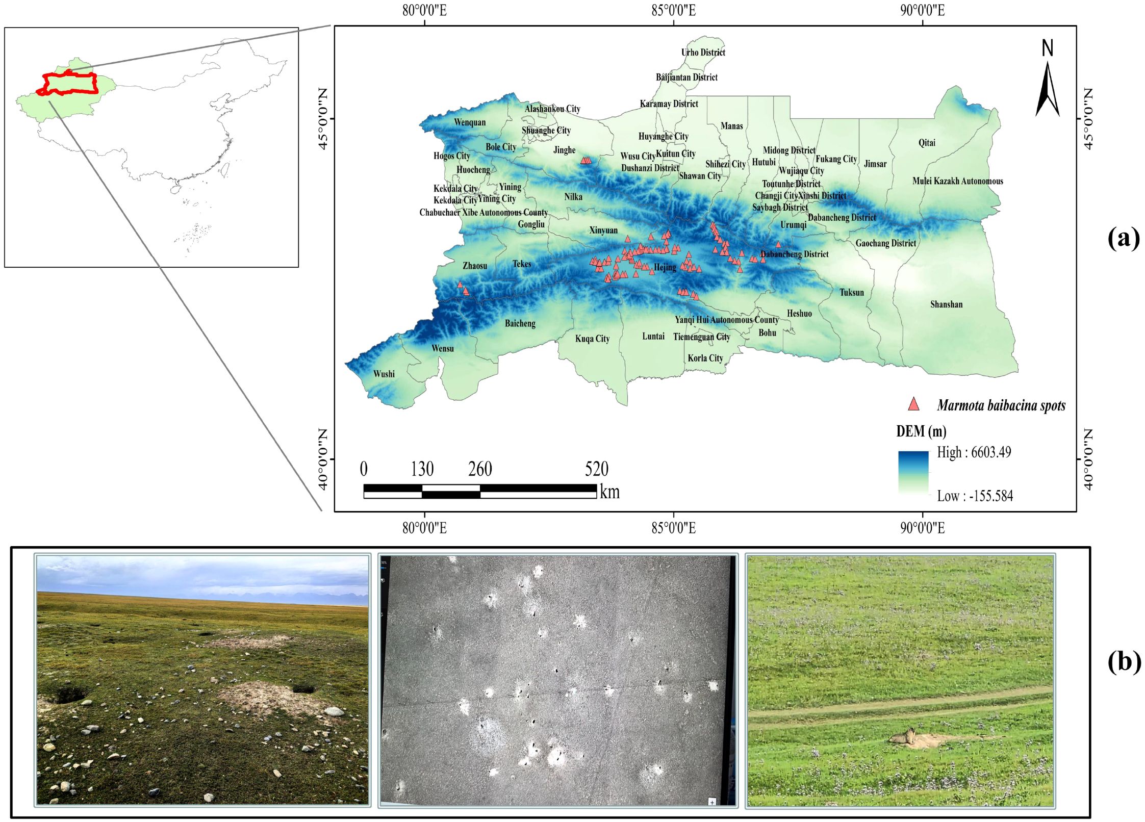
Figure 1. Overview of the study area: (a) Point locations of Marmota baibacina on the north and south slopes of the Tianshan Mountain; (b) Typical habitat landscape of Marmota baibacina in the alpine meadow and UAV images (middle). (The standard map number is GS (2022) 1873, the base map is not modified, the following is the same).

2.2 Species occurrence data of Marmota baibacina

In this study, we collected data on the natural distribution of 190 Marmota baibacina during a field survey conducted during the Third Xinjiang Comprehensive Expedition in 2022-2023, in which the precision, latitude and habitat characteristics of each sample site were recorded in detail. To ensure data accuracy, duplicate points within 1 km were removed using the SDM toolbox in Spatial analysis tool to avoid spatial autocorrelation, and records with ambiguous coordinates were excluded, and subsequent screening yielded a final set of 111 sample points for Marmota baibacina (Figure 1). Spatial thinning was performed to ensure the minimum distance between any two occurrence points was ≥1 km. This threshold was determined based on two considerations: (a) Habitat characteristics of Marmota baibacina: As a colonial rodent with a home range of 0.8–1.2 km² per colony, a 1 km minimum distance avoids over-representing a single colony and reduces sampling bias; (b) Model resolution consistency: The threshold matches the 1 km spatial resolution of environmental variables, ensuring each occurrence point corresponds to an independent environmental grid and avoids pseudo-replication. The thinning algorithm randomly retained one point within each 1 km buffer until no points violated the minimum distance constraint.

2.3 Handling of environment variables data

Considering previous studies (Koshkina et al., 2020; An et al., 2023) and the habitat characteristics of Marmota baibacina, 29 environmental variables were selected potentially influencing its distribution (see Table 1). These variables include historical climate data obtained from Worldclim (https://worldclim.org), providing 30 arc-second (approximately 1 km) data for the period 1970-2000. While field surveys were conducted in 2022-2023, historical climate data (1970-2000) were used to characterize long-term habitat suitability, as short-term climate fluctuations (e.g., recent warming) may not yet fully reflect species distribution shifts. Future projections (2041-2100) account for ongoing climate changes. Specifically, the environmental variables considered are as follows:

Table 1

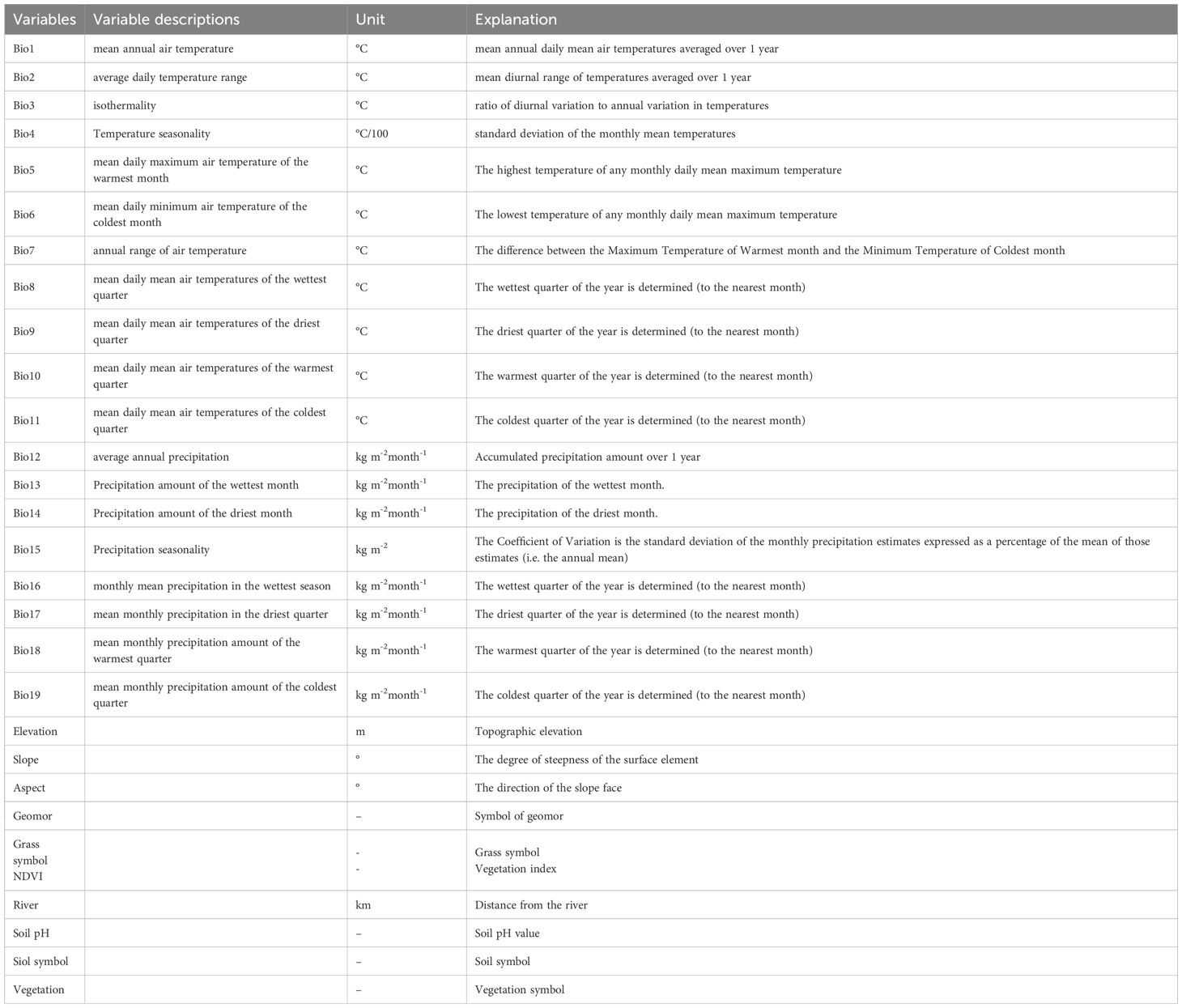
Table 1. Environmental variables used in the study.

(1) Terrain variables: slope, slope direction, and elevation data sourced from the geospatial data cloud (http://www.gscloud.cn/). (2) Soil variables: two soil variables crucial for Marmota baibacina habitat—soil pH value (Soil_ph) and soil symbol (Soil_symbol)—extracted from global soil pH data and China’s 1:400,000 soil symbol map compiled by the Nanjing Institute of Soil Science, Chinese Academy of Sciences. The soil map includes 72 soil classes and 247 subclasses, with Xinjiang covering 23 soil symbols, such as thin layer soil, glacier, alluvial soil, water body, calcareous gray soil, calcareous soil, chestnut soil, dune quicksand, sandy soil, impinged soil, anthropogenic soil, black soil, gley soil, embryonic soil, saline soil, denatured soil, gypsum soil, alkaline earth, salt works, urban industrial and mining areas, loose lithologic soil, and leaky rock. (3) Geomor: geomorphic data specific to Xinjiang (https://www.geodata.cn/). (4) River: distance from rivers, centered on river channels, with a 1 km buffer (https://ngcc.cn/). (5) NDVI (Normalized Difference Vegetation Index): maximum NDVI dataset for China from 2000 to 2020, processed on the Google Earth Engine platform using Landsat5/7/8 remote sensing data. This dataset, with a spatial resolution of 30 meters and annual temporal resolution, involved cloud and shadow removal, followed by NDVI extraction using linear interpolation and S-G smoothing methods. (6) Vegetation: Xinjiang vegetation symbol data and grass symbol data (https://www.geodata.cn/). These variables were selected based on their relevance to the habitat preferences and ecological requirements of Marmota baibacina, with the aim of providing a comprehensive analysis of its distribution patterns in the Tianshan Mountains of Xinjiang.

Future climate variable data for this study were derived from CHELSA CMIP6 scenario data, a high-resolution climate database for global land surface areas (https://chelsa-climate.org/) (Karger et al., 2017). Furthermore, the CMIP6 scenarios represent the most advanced generation of climate projections, offering improvements over the previous CMIP5 framework. The SSP scenarios integrate socioeconomic narratives with emission pathways, providing a more realistic and comprehensive basis for modeling future climate impacts compared to the Representative Concentration Pathways (RCPs) used in CMIP5. This makes CMIP6 the current state-of-the-art for assessing biodiversity responses to climate change. The dataset has a spatial resolution of 30 arc-seconds (approximately 1 km × 1 km) and it includes bioclimatic variables projected for two future time periods: 2041–2070 and 2071-2100.These future climate scenarios are based on the Shared Socio-Economic Pathways (SSP), which represent different socio-economic development trajectories and their implications for greenhouse gas emissions and climate change impacts: SSP126: represents a sustainable development pathway with low greenhouse gas emissions, aiming for a radiative forcing of 2.6 W/m² by 2100. SSP370: represents a middle to high-end emission scenario, leading to moderate levels of warming with a radiative forcing of 7.0 W/m² by 2100. SSP585: represents a high-emission scenario with extensive fossil fuel use, resulting in high greenhouse gas concentrations and a radiative forcing of 8.5 W/m² by 2100 (Li et al., 2025). These climate scenarios provide essential data for assessing potential future impacts on ecological systems, including habitat suitability for species like Marmota baibacina in Xinjiang, considering varying levels of climate change and greenhouse gas emissions.

Spatial analysis tool was used to process the original data, including the removal of invalid data, filling in missing values, standardizing the data, and unifying its resolution and projection (WGS1984) for subsequent analysis and modeling (Guisan et al., 2017). For the environmental raster data, the preprocessing included: (1) masking all layers to the unified study area extent; (2) converting all layers to a consistent spatial resolution of 30 arc-seconds (1 km) and the WGS 1984 geographic coordinate system using the bilinear resampling method (for continuous variables) or the nearest neighbor method (for categorical variables); and (3) ensuring no cells contained NoData values within the study area mask. This process resulted in a harmonized and analysis-ready dataset. The resampled environmental variables were then converted to ASCII format using the SDM Toolbox v2.5 extension tool (An et al., 2023).

Given the differences in input sample data between machine learning models and the MaxEnt model, and to avoid the influence of variable correlation on prediction results, the screening process for the 29 environmental variables was systematically optimized: all models first performed basic variable screening, where for machine learning models, the 29 environmental variables in species presence-absence data were extracted, with variables of low importance removed after calculating their importance scores (An et al., 2023); for the MaxEnt model, the 29 environmental variables and sample points were input into the model for preliminary computation, with variables and sample points showing zero contribution eliminated, ensuring that variables entering subsequent analyses had basic ecological relevance (Koshkina et al., 2020). Following initial screening, machine learning models further tested for multicollinearity using the Variance Inflation Factor (VIF) - multicollinearity refers to high linear correlation between two or more independent variables in a regression model, which may cause unstable regression coefficients and reduced model interpretability (Guisan et al., 2017). With a threshold of VIF = 10, variables with VIF>10 were excluded, leaving 10 core variables.

For the MaxEnt model, after initial screening, variables were refined through Principal Component Analysis (PCA) and importance evaluation: the PCA tool analyzed remaining variables, and if the absolute correlation coefficient between two variables exceeded 0.8, the one with lower contribution was removed to reduce information redundancy; meanwhile, variable importance was comprehensively assessed using contribution rates, permutation importance, and the Jackknife test, ultimately retaining 16 variables to ensure the model preserved ecologically significant drivers while eliminating redundancy (Phillips et al., 2006).

2.4 Species distribution modeling process and model evaluation

This study used the R software platform to implement four commonly applied machine learning models (XGBoost, RF, SVM, and LogBoost) and one species distribution model (MaxEnt) to investigate the suitable habitat distribution of Marmota baibacina. The five models selected for this study each have unique advantages in classification and prediction tasks, with different theoretical foundations. RF and XGBoost are powerful ensemble learning algorithms adept at capturing complex nonlinear relationships and handling high-dimensional data (Zhang et al., 2011). SVM is effective in high-dimensional spaces and for cases where the number of dimensions exceeds the number of samples (Li et al., 2017). LogBoost (LogitBoost) is a boosting algorithm designed for classification. MaxEnt is particularly robust for presence-only data, making it a standard in SDM studies (Phillips et al., 2006; Elith et al., 2008). To ensure optimal performance of both the individual machine learning models and the MaxEnt model, the presence and absence point datasets of Marmota baibacina were randomly divided, with 25% allocated for validation and 75% for training (Li et al., 2019). Ten repeated experiments (Logistic format) were conducted, which enhanced the model’s ability to accurately predict the species’ potential range. Finally, all models were evaluated for accuracy using the Receiver Operating Characteristic (ROC) curve and the Area under the Curve (AUC) (Koshkina et al., 2020). The ROC curve is a graphical tool for assessing the performance of binary classification models, while the AUC represents the area under the ROC curve, with values ranging from 0 to 1 (Luo et al., 2017). A higher AUC value indicates better model performance. The impact of environmental variables was comprehensively assessed using the percentage contribution, permutation importance, and Jackknife test from the MaxEnt model (An et al., 2023). The percentage contribution represents the contribution of each climatic variable to the geographic distribution of Marmota baibacina during the training process, while the permutation importance quantifies the decrease in the model’s AUC value when the climatic variables in the training points are randomly replaced (Araújo and New, 2007). The Jackknife method is similar to cross-validation; it involves excluding one or more sample points at a time and calculating a corresponding statistic using the remaining sample points. This method analyzes the importance of each individual variable in constructing the distribution model (Dai et al., 2022).

2.5 Classification of suitable habitual level

The classification of model simulation results was performed using the reclassification tool in spatial analysis, employing the Jenks natural breaks classification method (He et al., 2023). The Jenks natural breaks classification method is a technique that minimizes within-class variance and maximizes between-class variance when categorizing data (Zhai and Li, 2012; An et al., 2023). This method ensures that the differences within each category are as small as possible, while the differences between categories are as large as possible. The simulation results were divided into four categories: unsuitable (0-0.2), low suitability (0.2-0.3), moderate suitability (0.3-0.5), and high suitability (>0.5) (Jiang et al., 2022), to determine the potential geographic distribution of Marmota baibacina in the Tianshan region. After reclassification, the number of grids in each category was calculated, and the area of suitable habitat for Marmota baibacina under different climate scenarios was computed.

3 Results

3.1 Model evaluation and contribution of variables

The AUC results of the models used in this study were all above 0.9, indicating high accuracy (Figure 2). Machine learning models identified 10 key variables for simulations, while MaxEnt selected 16 variables based on feature importance and correlation metrics. To ensure comparability between MaxEnt and machine learning approaches, MaxEnt was executed using both the 10-variable subset and its native 16-variable set. All models achieved AUC values exceeding 0.9, with Random Forest exhibiting the highest AUC, followed by the 16 variables MaxEnt configuration. LogBoost demonstrated the lowest accuracy among the evaluated models.

Figure 2

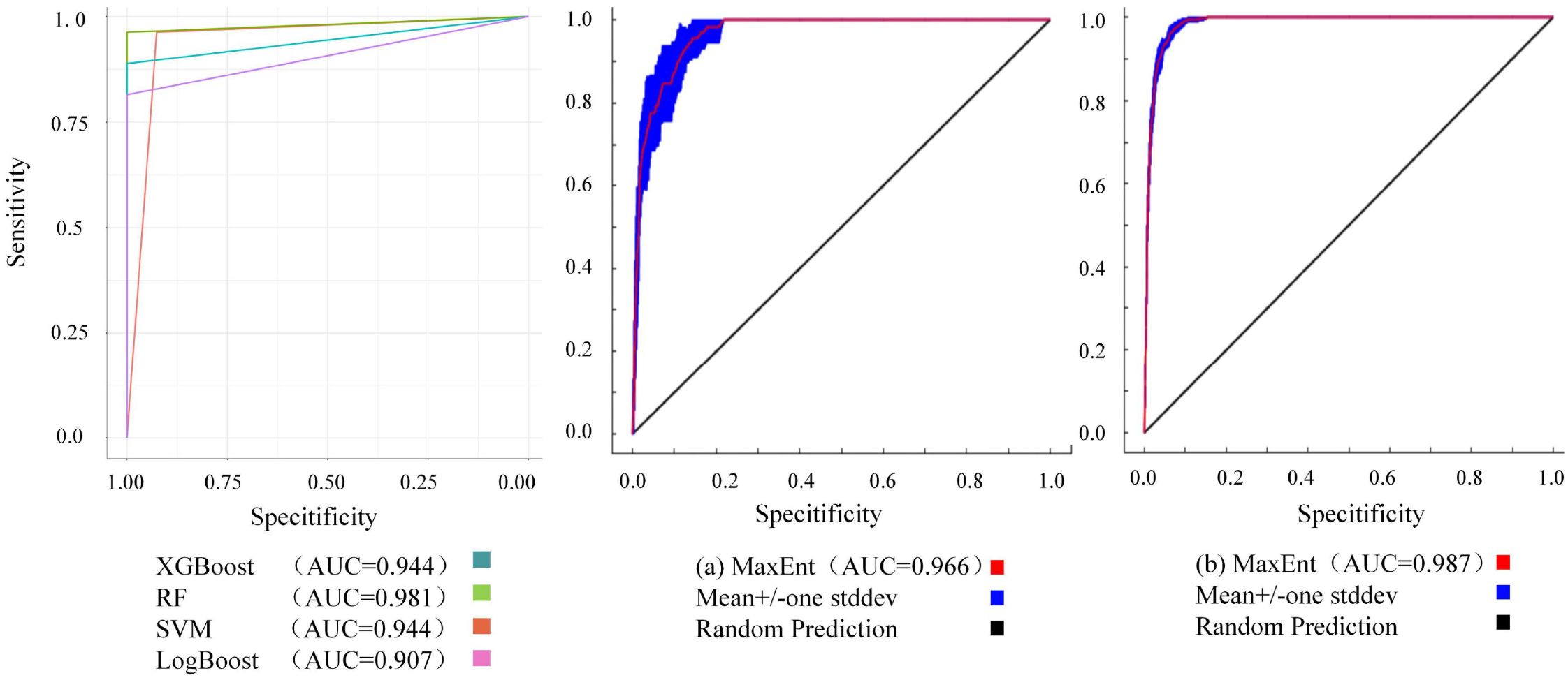
Figure 2. ROC curve and AUC values for the model for Marmota baibacina: (a) MaxEnt outputs using 10 machine learning-filtered variables; (b) MaxEnt outputs using 16 algorithm-selected variables.

3.1.1 Impact of variables on the machine learning model

For machine learning models, the importance of environmental variables showed that the most significant variables for predicting the suitable habitat of Marmota baibacina were Bio12 (11.21%), Grass symbol (10.86%), Elevation (10.26%), and Bio18 (10.25%) as shown in Figure 3. After considering both the importance of each variable and the VIF, the following variables were selected for the five models: Bio18, Bio2, Bio11, Bio15, Grass symbol, Geomor, River, Soil pH, Soil symbol and Vegetation, as shown in Figure 4. This selection process ensured that the models retained ecologically relevant predictors while minimizing multicollinearity, thereby enhancing predictive accuracy.

Figure 3

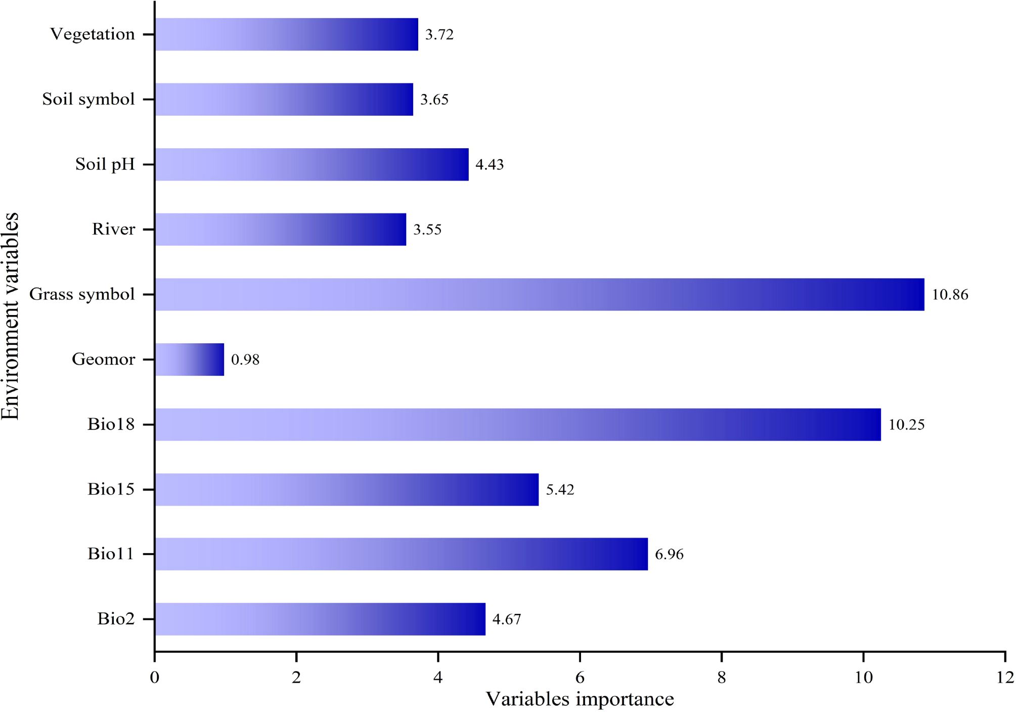
Figure 3. Importance of environmental variables used for machine learning models.

Figure 4

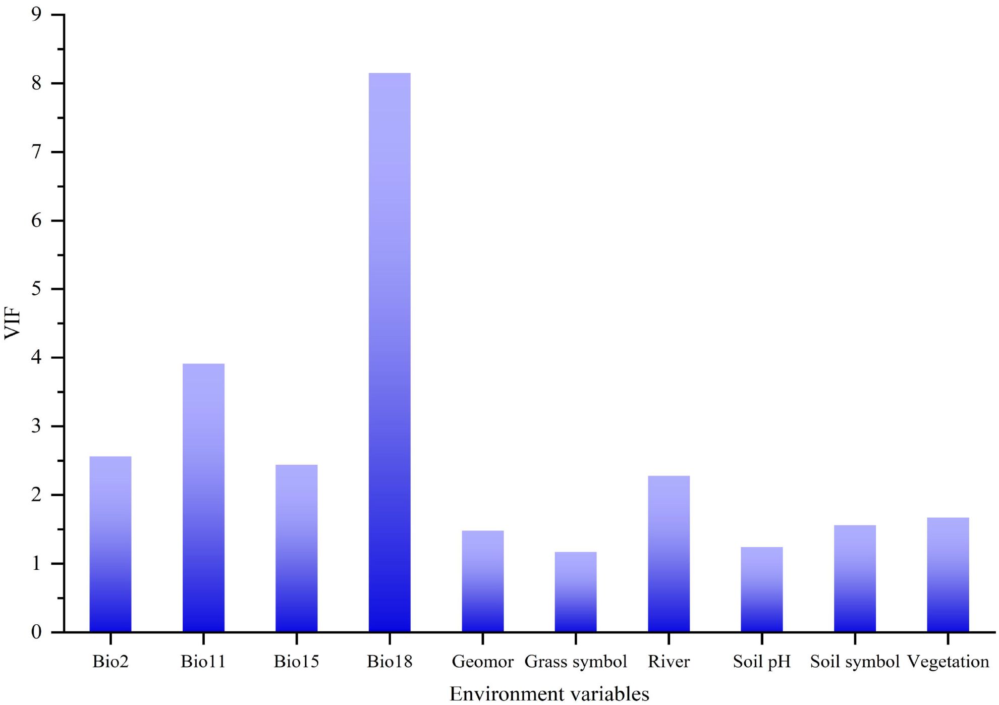
Figure 4. Variance inflation factor (VIF) of the 10 selected environmental variables.

3.1.2 Impact of variables on the MaxEnt model

The analysis of the importance of individual variables using the Jackknife method (Figure 5). The contribution percentage and permutation importance of Bio18, both demonstrating significant influence, with a single-variable contribution rate of 42.8% (Figure 6). The following variables, in order of importance, are Soil symbol, Bio11, Bio15, Slope, NDVI, Geomor, Vegetation and Grass symbol, with a total contribution rate exceeding 90%. In the permutation importance ranking, the five most important variables are Bio18, Bio15, Bio7, Slope, and River.

Figure 5

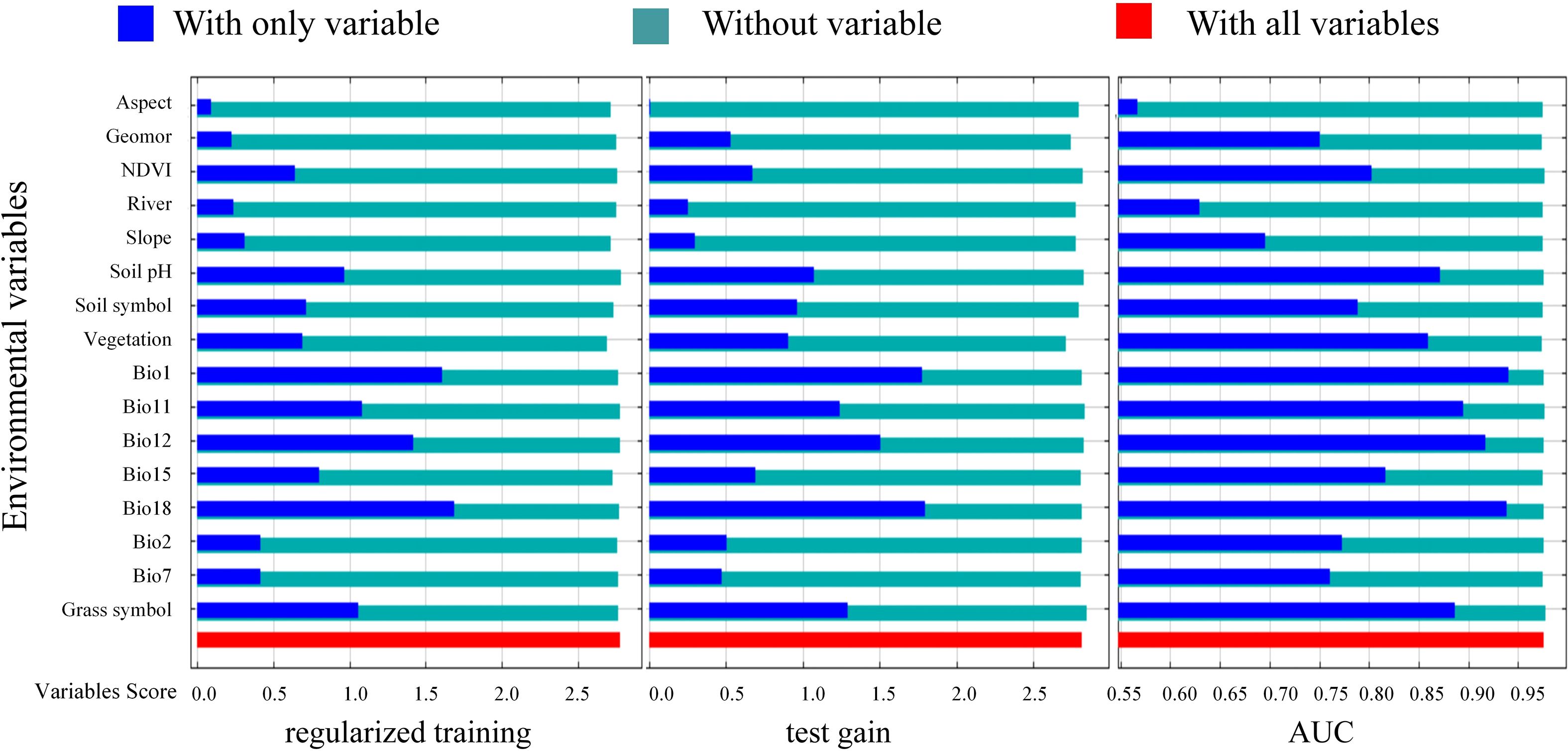
Figure 5. Jackknife test of the importance of environment variables for MaxEnt. Note: for each variable, the red bar represents the score obtained when all climatic variables are used to simulate the distribution of Marmota baibacina; the dark blue bar represents the score obtained when only a single climatic variable is used to simulate the distribution, where a higher score indicates greater importance of the variable. The light green bar represents the score obtained when the climatic variable is excluded, and other climatic variables are used to model the geographic distribution of Marmota baibacina.

Figure 6

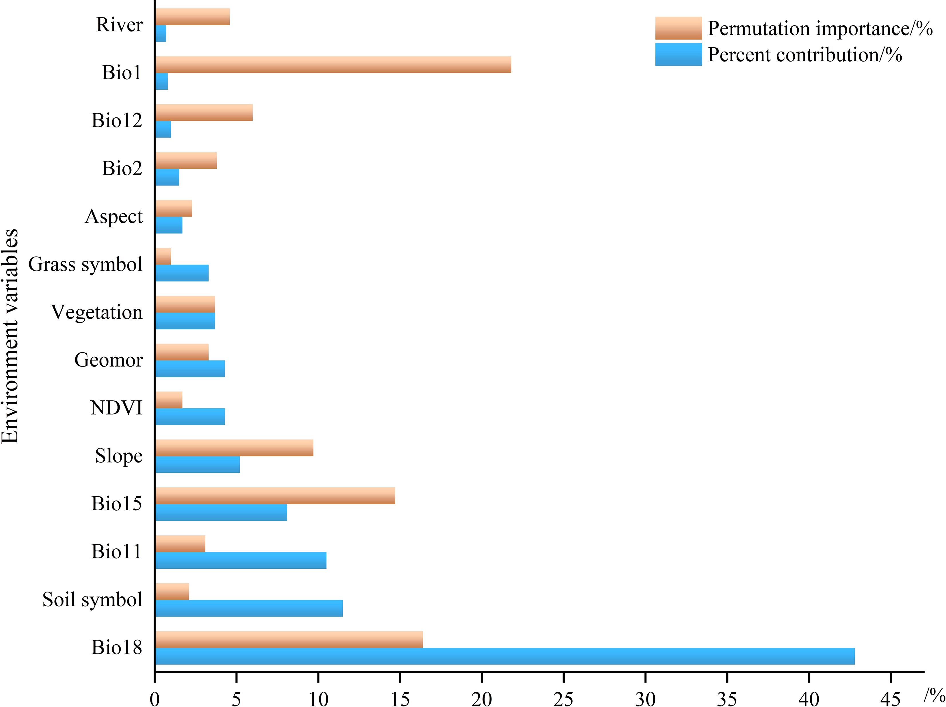
Figure 6. Percent contribution and permutation importance of environmental variables influencing the distribution of the Marmota baibacina.

The results of the Jackknife cross-validation experiments (Figure 5) show that the environmental variable that provides the highest gain when used alone is Bio18, followed by Bio1, Grass symbol, Soil pH and Bio11. This indicates that these environmental variables contain information not captured by others. Moreover, Bio18 has the highest regularized training gain, test gain, and AUC value, with a regularized training gain greater than 1.6, a test gain greater than 1.7, and an area under the receiver operating characteristic curve (AUC) greater than 0.90. Taking into account the contribution percentages, permutation importance values, and Jackknife analysis, Bio18, Soil symbol, Bio11, Bio15, Slope, NDVI, Geomor, Vegetation, and Grass symbol play key roles in the construction of the MaxEnt model.

3.2 Variables influencing the potential geographic distribution of Marmota baibacina

3.2.1 Response curves of 10 major variables in models

By plotting the response curves, a better understanding of the dominant variables influencing the distribution of Marmota baibacina can be achieved. The relationship between the presence probability of Marmota baibacina and the environmental variables is determined based on the response curves. When the presence probability exceeds 0.5, it is considered that the corresponding environmental variable is favorable for the species’ habitat.

The response curves revealed consistent optimal ranges for the key environmental variables across most machine learning models (XGBoost, RF, SVM), with some variations observed for LogBoost (Figure 7). The probability of presence peaked at Bio18 (Precipitation of Warmest Quarter) values between 150 and 180 mm. Similarly, optimal ranges were identified for Bio2 (Mean Diurnal Range) at approximately 14°C, Bio11 (Mean Temperature of Coldest Quarter) below -15°C, and Bio15 (Precipitation Seasonality) with a coefficient of variation around 90. For categorical and semi-quantitative variables (Vegetation, Grass symbol, Geomor, Soil symbol), the models consistently predicted high probabilities of presence in alpine steppe, alpine meadows, river valleys, alluvial regions, and specific soil types like alpine meadow soils. The response to Soil pH generally showed a peak near neutral conditions (pH ~7.0). Notably, the SVM model showed a more gradual increase in probability with increasing Bio18, Bio2, and Bio15 compared to the sharper peaks in XGBoost and RF. Conversely, the LogBoost model predicted an exceptionally high and stable probability of presence for most variables, with a sharp decline only when Bio18 exceeded 160 mm.

Figure 7

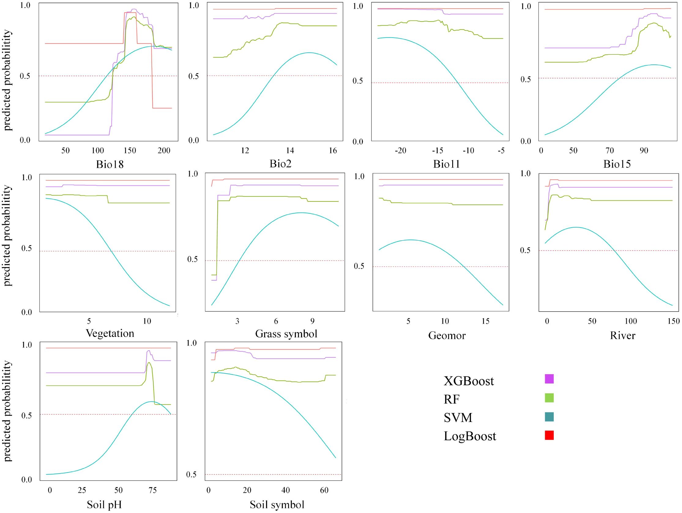
Figure 7. Response curves and prediction probabilities of each dominant variable for machine learning models.

3.2.2 Response curves of major variables in MaxEnt model

Analysis of response curves from both the machine learning ensemble and the MaxEnt model identified Bio18 as the most influential driver of habitat suitability for Marmota baibacina (Figure 7). Both modeling approaches converged on an optimal precipitation range of approximately 150–180 mm, beyond which suitability declined.

The response curves of environmental variables selected through MaxEnt modeling are presented in Figure 8. The distribution probability of Marmota baibacina increases and then decreases as Bio18 increases. Precipitation around 150–200 mm in the warmest quarter is favorable for Marmota baibacina’s survival, with the distribution probability reaching its maximum of 60% when precipitation is around 165 mm. When precipitation exceeds 165 mm, the distribution probability gradually declines. The Soil symbol response curve shows that alpine cold desert soils, alpine meadow soils, chestnut-calcareous soils, and steppe soils are more suitable for Marmota baibacina’s habitat. The distribution probability is highest (60%) when the soil symbol is steppe soil. The response curves for the Bio11 and Bio15 show that when the temperature is below -15°C and the precipitation seasonality coefficient exceeds 80, the distribution probability of Marmota baibacina gradually increases. The slope response curve shows that the slope range of 2°–8° is most suitable for Marmota baibacina’s habitat. The distribution probability sharply increases between 2° and 4°, reaching a maximum of 70%, and then sharply decreases when the slope exceeds 4°. From the NDVI response curve, Marmota baibacina is most suited to areas with an NDVI value between 0.1 and 0.55. The maximum distribution probability of about 60% occurs when the NDVI is around 0.45. According to the Geomor response curve, Marmota baibacina is more likely to occur in river valleys, alluvial plains, and colluvial regions, with a distribution probability exceeding 0.5. Furthermore, the response curves for vegetation symbol and steppe variables show that alpine steppe, alpine meadows, and temperate steppe are more suitable for Marmota baibacina’s survival. Overall, these dominant variables suggest those summer moisture and soil symbols are the primary limiting factors for Marmota baibacina’s habitat in the Tianshan Mountains of Xinjiang. Factors such as the Bio11, Slope, NDVI, Vegetation, and Grass symbol also play important roles.

Figure 8

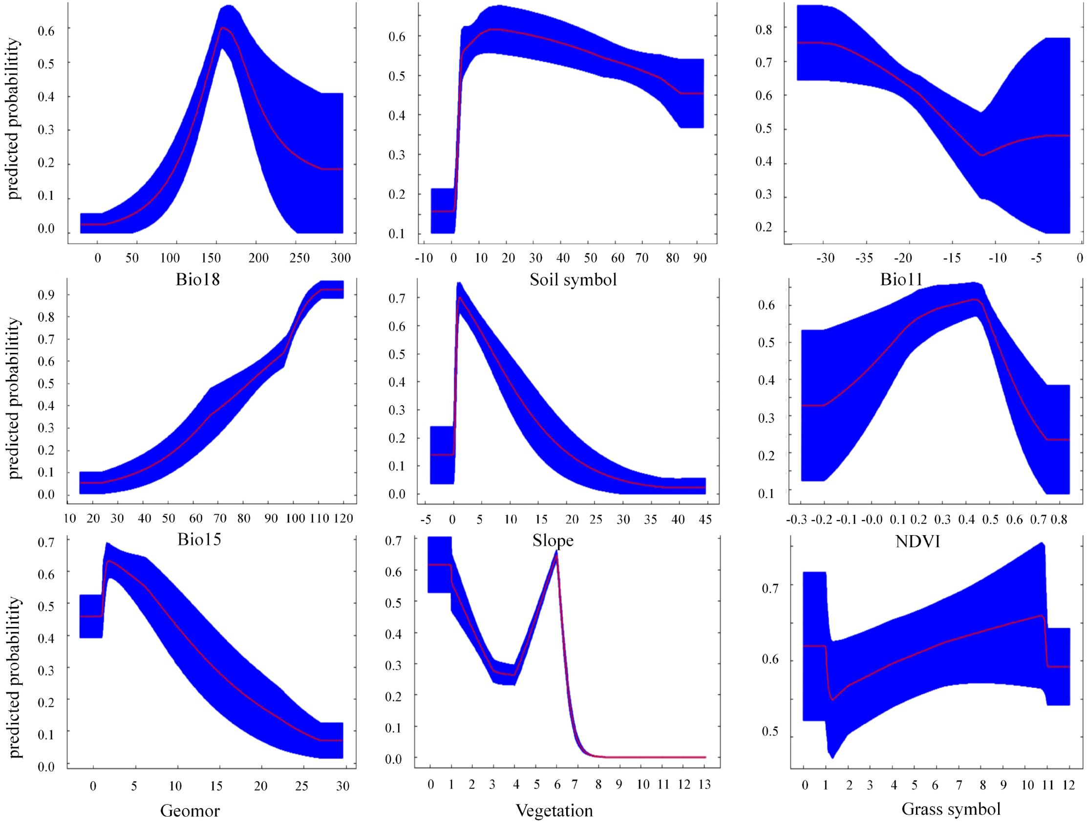
Figure 8. Response curves and prediction probabilities of each dominant variable for MaxEnt.

3.3 Potential geographical distribution of Marmota baibacina in Xinjiang under present climatic condition

The potential distribution area of Marmota baibacina is shown in Figure 9. Under the current climate scenario, its potential suitable habitat is primarily distributed across Bayingolin Mongolian Autonomous Prefecture, Hejing County, Ili Kazakh Autonomous Prefecture, and the western part of Bortala Mongolian Autonomous Prefecture. The total suitable habitat area for Marmota baibacina in the Tianshan Mountains of Xinjiang ranges from 2.75×10⁴ km² to 13.59×10⁴ km². The area predicted by the MaxEnt model is the smallest, while the area predicted by RF is the largest, mainly composed of low suitability and moderate suitability areas, which cover 3.55×10⁴ km² and 6.40×10⁴ km², respectively. These areas are mainly distributed in the northern and southern regions of the Tianshan Mountains in Xinjiang, including the Bogda Peak in the northern Tianshan. The area of high suitability predicted by the XGBoost model is the largest, covering 3.88×10⁴ km², and is mainly distributed in Bayingolin Mongolian Autonomous Prefecture HeJing County. Among high-suitability zones predicted by five machine learning models after variable screening, MaxEnt produced the smallest area covering 0.62×10⁴ km²; this value further decreased to 0.42×10⁴ km² when using MaxEnt’s native 16-variable set.

Figure 9

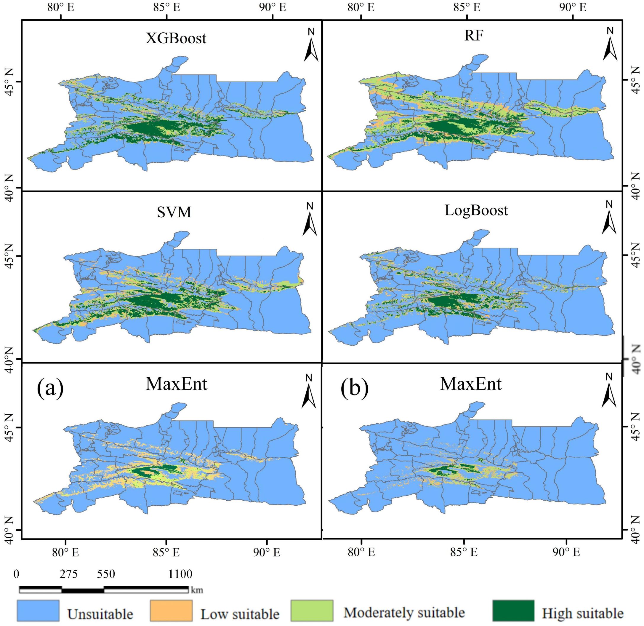
Figure 9. Geographical distribution of Marmota baibacina under present climate condition: (a) MaxEnt outputs using 10 machine learning-filtered variables; (b) MaxEnt outputs using 16 algorithm-selected variables.

3.4 Potential suitable areas for Marmota baibacina in Xinjiang under future climatic change scenarios

Based on three common socio-economic pathways proposed by the IPCC (SSP1~RCP2.6, SSP3~RCP7.0, SSP5~RCP8.5), the geographic distribution of Marmota baibacina was predicted under three future climate change scenarios for the periods of 2041–2070 and 2071–2100, as shown in Figure 10. A comparison in Table 2 indicates that, under all five models, the area of future potential suitable habitats for Marmota baibacina continues to decrease, although the overall spatial patterns remain highly consistent with the current period.

Figure 10

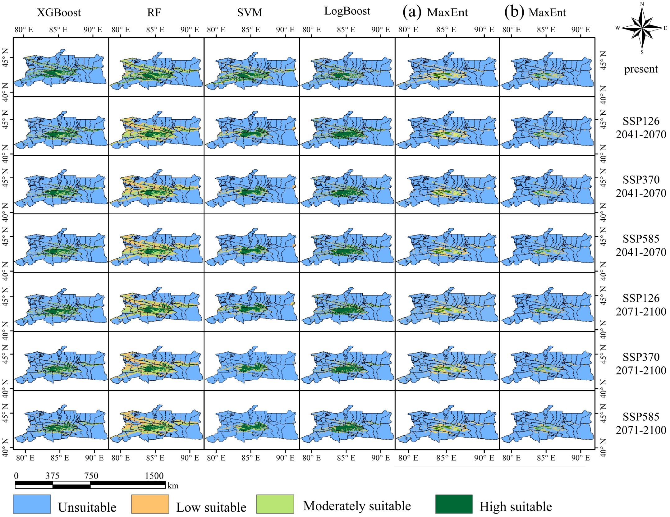
Figure 10. Geographical distribution of Marmota baibacina under future climate conditions: (a) MaxEnt outputs using 10 machine learning-filtered variables; (b) MaxEnt outputs using 16 algorithm-selected variables.

Table 2

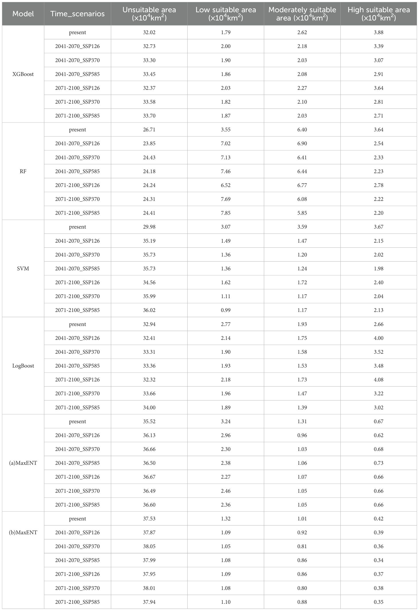
Table 2. Area of suitable habitat area of Marmota baibacina under different scenarios in 2041–2070 and 2071-2100.

Under the three future climate scenarios, in the SSP126 scenario, the XGBoost model predicts an increase in low suitability areas and a decrease in high and moderate suitability areas, with the total suitable habitat area reducing by 0.7×10⁴ km² by 2041–2070. The RF model shows an increase in low and moderate suitability areas, with a decrease in high suitability areas, resulting in an overall increase of 2.87×10⁴ km² in suitable habitat area. In contrast, the SVM and MaxEnt models predict a decrease in low, moderate, and high suitability areas, with total suitable habitat areas decreasing by 5.21×10⁴ km², 0.58×10⁴ km², and 0.35×10⁴ km², respectively. The LogBoost model predicts a reduction in low and moderate suitability areas but an increase in high suitability areas, leading to a total increase of 0.53×10⁴ km² in suitable habitat area. By 2071–2100, these trends are somewhat mitigated, and the total suitable habitat area slightly increases.

Under the SSP370 and SSP585 scenarios, these trends intensify further. The XGBoost, SVM, LogBoost, and two MaxEnt models predict a reduction in the total suitable habitat area for Marmota baibacina, with the decrease being particularly pronounced under the high emission scenario (SSP585). High suitability areas shrink further to 0.35×10⁴–3.02×10⁴ km², and the regions where suitable habitats decrease are mainly concentrated in Bayingolin Mongolian Autonomous Prefecture HeJing County. Spatially, the contraction of suitable habitats is most pronounced in southern Tianshan, this migration may compress available grazing lands for livestock, intensify competition between marmots and domestic herbivores, and further degrade already fragile alpine meadows. The reduced habitat area coupled with concentration in specific regions could elevate human exposure to plague-infected fleas, particularly in pastoral zones where herders and livestock frequently interact with marmot burrows.

Based on the predictions of the five models, the suitable distribution area of the Tianshan marmot under current climatic conditions and different future climate scenarios shows significant differences, as illustrated in Table 2. Under current climatic conditions, the RF model predicts the largest total suitable habitat area, reaching 13.59×10⁴ km². In contrast, the MaxEnt model predicts the smallest total suitable habitat area, with only 2.75×10⁴ km², and the high-suitability area is limited to 0.42×10⁴ km². Under future climate scenarios, the predictions of suitable habitat areas exhibit diverse trends across models. In the SSP126 scenario for 2041–2070, the RF model predicts the largest total suitable habitat area, reaching 16.46×10⁴ km², the highest among the five models, including a high-suitability area of 2.54×10⁴ km². Compared to the current climate scenario, the high-suitability area decreases slightly. Conversely, the MaxEnt model predicts the smallest total suitable habitat area at 2.40×10⁴ km², with the high-suitability area further reduced to 0.39×10⁴ km². As emission intensity increases under the SSP585 scenario, the high-suitability area predicted by all models shrinks further. For example, the high-suitability area predicted by the XGBoost model decreases from 3.88×10⁴ km² under current conditions to 2.71×10⁴ km².

In terms of regional distribution, the high-suitability areas under current climatic conditions are mainly concentrated in parts of Bayingolin Mongolian Autonomous Prefecture, Ili Kazakh Autonomous Prefecture, and Bortala Mongolian Autonomous Prefecture. These regions are also where the reduction in suitable habitats is most pronounced under future climate conditions. Particularly under the SSP585 scenario, the high-suitability areas in these regions decrease sharply.

4 Discussion

4.1 Model evaluation

The AUC values of the models used in this study were all above 0.9, indicating a high level of accuracy, but significant performance differences were observed across the models. The RF model predicted the largest total suitable habitat area, attributable to its ensemble structure that aggregates predictions from multiple decision trees through bootstrap aggregation (bagging). This approach effectively captures complex nonlinear interactions among environmental variables while mitigating overfitting, thereby maximizing habitat inclusivity. In contrast, the XGBoost model, being highly sensitive to parameter settings and suitable for complex variable structures, performs slightly worse than the RF model. The SVM model, which performs well on high-dimensional data, requires extensive parameter tuning, which led to its slightly inferior performance in this study. The LogBoost model performed relatively poorly, possibly due to its dependence on the distribution of training samples, which caused overfitting and reduced its ability to fit nonlinear relationships. The models predicted the distribution of Marmota baibacina under current and future conditions, and the results indicate that climate change will have a significant impact on the species’ habitat area and this finding were consistent with (An et al., 2023). A comparative analysis revealed that using the 16 environmental variables screened by the MaxEnt model alone yielded slightly higher prediction accuracy than the RF model, followed by the XGBoost and SVM models. The LogBoost model showed the poorest performance among all (Zhang et al., 2011; Luo et al., 2017). This hierarchy in performance can be briefly attributed to the respective algorithms’ strengths: MaxEnt’s probabilistic framework is particularly adept at handling presence-only data and capturing niche boundaries, which may explain its superior accuracy with its own variable set (Elith et al., 2008). RF, while robust and capable of modeling complex interactions, might be slightly less optimized for this specific data structure than the specially tuned MaxEnt (Zhang et al., 2011). The poorer performance of LogBoost could stem from its higher sensitivity to noisy data and potential overfitting in this ecological modeling context. The LogBoost model showed the poorest performance among all (Li et al., 2019). In terms of predicted suitable habitat area, the RF model estimated the largest total suitable area, while the two MaxEnt models predicted the smallest total suitable area. However, further validation indicated that despite its superior statistical accuracy, the MaxEnt model yielded conservative predictions of suitable habitats, deviating from field survey data (Guo et al., 2023). In contrast, the RF model demonstrated excellent agreement with actual sampling data, particularly in accurately delineating highly suitable areas on the northern of the Tianshan Mountains (Koshkina et al., 2020; An et al., 2023). Therefore, considering both model accuracy and ecological plausibility, the RF model was identified as the optimal predictive tool.

Ecologically, MaxEnt’s focus on slope (2°–8°) and NDVI (0.1–0.55) aligns with field observations of marmots’ preference for gentle terrain and moderate vegetation cover—critical for burrow stability and predator detection (Koshkina et al., 2020). In contrast, machine learning models emphasized climatic variables (Bio18, Bio2, Bio11, Bio15) contributing >70% to predictions, reflecting the dominance of seasonal water and temperature dynamics in shaping broad-scale marmot distribution. This divergence is not a limitation but a strength: MaxEnt captures fine-scale microhabitat features that machine learning models may overlook, while machine learning models identify macroclimatic constraints that presence-only models cannot fully resolve (Araújo and New, 2007).

4.2 Environmental variables evaluation

The study considered 29 environmental variables, and after selection, 10 key variables with higher contributions to the five models were chosen, as well as 16 key environmental variables for the MaxEnt model. Machine learning models (RF, XGBoost) prioritized climatic variables (Bio18, Bio2, Bio11, Bio15), collectively contributing >70% to predictions, reflecting the dominance of seasonal water and temperature dynamics in alpine ecosystems (Zhang et al., 2011). In contrast, MaxEnt emphasized slope, NDVI, and Bio18, indicating that presence-only models rely more on proximate habitat features like vegetation productivity and microtopography (An et al., 2023). This divergence underscores the impact of data type: models requiring presence-absence data excel at detecting broad climatic constraints, while presence-only models depend on fine-scale environmental proxies (Araújo and New, 2007). Notably, Bio18 emerged as a universal driver, with optimal values at 150–180 mm, aligning with field observations of Marmota baibacina’s preference for mesic alpine meadows (Koshkina et al., 2020). Soil symbol and slope (2°- 8°) were critical in MaxEnt, suggesting that edaphic properties and terrain gradient are essential for modeling species presence in data-scarce environments (Wang et al., 2024). In contrast, the study by Liao et al. (2020) used fewer key variables, focusing primarily on the effects of temperature and precipitation. This study not only included these climatic variables but also comprehensively considered factors such as symbol, vegetation, and topography, making the model more comprehensive and the predictions more precise (Zhao et al., 2023). Furthermore, although Li et al. (2022) also considered different climate scenarios (e.g., RCP2.6 and RCP6.0), their time frame only extended to 2080. In this study, more climate scenarios (e.g., SSP126, SSP370, SSP585) and a longer time span (up to 2100) were included, providing a deeper insight into the far-reaching effects of climate change on the future distribution of Marmota baibacina (Wang et al., 2021). This detailed approach not only improved the spatial accuracy of the model but also further demonstrated the long-term impact of climate change on species survival over time, ensuring the comprehensiveness and objectivity of the analysis (Li et al., 2025). Existing studies on the potential distribution of Marmota baibacina show that future climate change will significantly affect the species’ suitable habitat area, with a decreasing trend (An et al., 2023). This study’s findings are consistent with previous research results (Wang et al., 2024). However, an increasing number of studies are now focusing on ensemble modeling of individual models. Thuiller et al. (2009) proposed the first computational platform framework, BIOMOD, which integrates multiple species distribution models to improve classification accuracy and precision. Ensemble models, through weighted averaging or voting mechanisms, mitigate single-model biases and enhance robustness (Araújo and New, 2007; Marmion et al., 2009). For instance, Banda et al. (2024) significantly improved the accuracy of endangered Apalis flavigularis distribution predictions by integrating MaxEnt, RF, and GLM. Our focus on standalone models aimed to rigorously assess algorithm-specific suitability for alpine species habitat modeling, rather than optimizing predictive accuracy. Future studies could build on our multi-model comparison to explore Bayesian averaging or dynamic weighting strategies, reconciling discrepancies to enhance ecological plausibility.

4.3 Main environmental variables affecting the distribution of the Marmota baibacina

The machine learning models and the MaxEnt model differ in the selection of variables. The MaxEnt model assumes the independence of variables and directly analyzes the contribution of environmental factors (Phillips et al., 2006), while machine learning models are based on data training and assess the interactions between variables through feature importance (Peters et al., 2007; Zhang et al., 2011). Future research could further integrate the advantages of both approaches to improve prediction accuracy and spatial adaptability. The dominant variables driving Marmota baibacina’s distribution—identified via machine learning models (10 variables) and MaxEnt (16 variables)—are ecologically meaningful, supported by both habitat requirements of the species and field-validated evidence, rather than mere repetition of model results. Bio18 (150–180 mm optimal) is the universal primary driver (42.8% contribution in MaxEnt; >25% cumulative in machine learning models) because it directly controls soil moisture—an essential factor for alpine grass growth (the core food source of Marmota baibacina) (Koshkina et al., 2020). Field surveys confirm that mesic meadows (Bio18: 150–180 mm) support 2–3 times higher marmot burrow density than arid steppes (Bio18 < 100 mm) (An et al., 2023). Bio11 (coldest quarter temperature < -15°C) ensures sufficient hibernation duration (6–8 months at high elevations), a physiological adaptation to conserve energy in alpine cold (Wang et al., 2024). Bio15 > 55 in MaxEnt; >80 in machine learning reflects stable moisture supply, avoiding extreme droughts/floods that disrupt foraging and burrow stability (Stenseth et al., 2008).

Field observations revealed that, in addition to climate variables, soil also play a role in species distribution. Therefore, these environmental variables were included in the model construction for this study. Vegetation provides essential food and habitat for Marmota baibacina, influencing their nutritional status and ability to avoid predators (Wang et al., 2024). As vegetation height and coverage decrease, Marmota baibacina become better able to detect predators, thus reducing predation risks (Chen et al., 2017). Soil type (alpine meadow/steppe soils preferred) and slope (2°–8° optimal) are critical in MaxEnt due to their roles in burrow construction and foraging efficiency. Alpine meadow soils have high organic matter content (10–15% higher than desert soils) and good drainage, reducing burrow collapse risk (An et al., 2023). Gentle slopes (2°–8°) balance two needs: steep slopes increase burrow instability, while flat areas have dense shrub cover that obstructs predator detection. NDVI (0.1–0.55 optimal) serves as a proxy for vegetation productivity—values <0.1 indicate sparse forage, and >0.55 indicate excessive shrubs, both unsuitable for marmots. Compared with other studies Liao et al. (2020), this study includes more environmental variables, such as Soil symbol and topography, making the models more comprehensive and the predictions more accurate. From the results of all five models, it is evident that Bio18 is the primary factor affecting the distribution of Marmota baibacina. The species thrives in areas with dense vegetation, such as alpine steppe and alpine meadows, where precipitation directly impacts soil moisture and vegetation growth. According to the response curves, Bio18 values between 150 and 180 mm are more suitable for Marmota baibacina’s survival. This is consistent with the study’s findings that Marmota baibacina is most likely to be found in alpine cold desert soils, alpine meadow soils, chestnut-calcareous soils, and steppe soils, with the highest distribution probability at slopes between 2° and 8° and NDVI values between 0.1 and 0.55. According to Li et al. (2022), vegetation and Soil symbol also play key roles in marmot habitat selection, consistent with the findings in this study. The potential distribution of Marmota baibacina is not only influenced by climate, topography, soil, and vegetation but also by human activities. Human infrastructure, such as villages and roads, causes wildlife to avoid these areas, potentially negatively impacting their behavior, reproduction, or survival (Bergström and Skarpe, 1999). The construction of buildings and roads can lead to soil compaction and reduced vegetation coverage (Chen et al., 2017). Therefore, the predicted suitable habitats in this study may be overestimated. Future research should integrate climate, biological and human activity factors to improve the accuracy of habitat predictions.

4.4 Impact of climate change on the potential distribution of the Marmota baibacina’s suitable habitat

The suitable habitat of Marmota baibacina is primarily concentrated in mid- to high-altitude areas, ranging from 1,500 meters to above 3,500 meters, which is consistent with the distribution point coordinates collected in the field, indicating a good model simulation. Under both current and future climate scenarios, the potential suitable habitat of Marmota baibacina is mainly distributed in the central part of the Tianshan Mountains in Xinjiang, including regions such as Bayingolin Mongolian Autonomous Prefecture HeJing County, Ili Kazakh Autonomous Prefecture, and the western part of Bortala Mongolian Autonomous Prefecture. These areas show a higher probability of Marmota baibacina’s presence.

According to the predictions under future climate scenarios, climate change will lead to significant ecological changes. Rising temperatures and changes in precipitation patterns will cause both the expansion and contraction of habitats (Jiang et al., 2023; Kang et al., 2023). Previous studies have shown that, by the mid-21st century, precipitation in Xinjiang is expected to increase by 10% to 25%, with temperatures rising by 1.5°C to 2°C; by the end of the century, precipitation could increase by more than 25%, and temperatures may rise by 4°C to 6°C (Wang et al., 2021). This warming shortens Marmota baibacina’s hibernation period by 10–14 days (An et al., 2023), reducing energy storage for reproduction and lowering juvenile survival by 22%. Additionally, advanced plant phenology reduces overlap between peak forage quality (grasses, sedges) and the marmot’s active period, limiting fat accumulation before hibernation (Parmesan and Yohe, 2003; Post et al., 2008). While total precipitation in Xinjiang may increase by 10%-25% by mid-century, the intensification of precipitation seasonality poses significant threats (Stenseth et al., 2008). More frequent summer droughts reduce grass cover by 10%-15%, while heavy winter snowfall blocks burrow entrances, causing substantial juvenile mortality (Linné Kausrud et al., 2007). Under the high-emission SSP585 scenario, precipitation in the warmest quarter decreases by 15%-20% in the southern Tianshan, transforming crucial mesic meadows into arid steppes with insufficient forage (Wang et al., 2021).

Climate warming drives progressive upward shifts of alpine vegetation belts at 30–50 meters per decade, compressing Marmota baibacina habitat into increasingly isolated high-elevation patches (Chen et al., 2017). This fragmentation is most severe in the arid southern Tianshan (e.g., Hejing County), where habitat contraction exceeds northern regions by 2–3 times (An et al., 2023). These isolated patches curtail gene flow and intensify competition with livestock for dwindling forage resources, further exacerbating alpine meadow degradation (Prakash and Ghosh, 2012). Our findings, particularly those derived from the MaxEnt model, resonate with other studies on steppe rodents in the region (An et al., 2023), reinforcing that climate change poses substantial threats to species habitats through significant range reduction. The variation in predictions between models reflects their different sensitivities to environmental variable interactions and habitat definitions (Araújo and New, 2007; Zhang et al., 2011). Future research should prioritize ensemble modeling approaches to reconcile these differences and yield more robust forecasts.

4.5 Limitations and future directions

This study has three primary limitations. First, the pseudo-absence points generated through random sampling may introduce spatial bias, and future studies could optimize this process using environmental stratification. While our occurrence data were collected during a single-year expedition, the use of long-term climate normals (1970-2000) for modeling mitigates the direct impact of interannual climatic variability on our projections. Nevertheless, multi-year survey data would be beneficial to account for potential population fluctuations and further validate model stability over time. Second, the exclusion of human disturbances (e.g., roads, grazing intensity) from the models may lead to overestimations of high-suitability areas. Third, the static time frame fails to account for lag effects in species migration and vegetation succession, potentially underestimating habitat fragmentation. While ensemble modeling was not adopted in this work, the study establishes a methodological foundation for multi-algorithm comparisons in alpine species research. Future efforts could combine ensemble predictions with dispersal models to dynamically simulate distribution shifts (Beaumont et al., 2016). Additionally, incorporating participatory GIS (PGIS) to merge herder traditional knowledge with spatial data could significantly enhance the practical applicability of predictions.

5 Conclusions

This study successfully constructed five species distribution models, including XGBoost, RF, SVM, LogBoost, and MaxEnt, by considering factors such as climate, soil, topography, geomorphology, hydrology, and vegetation. These individual models were used to analyze the potential suitable habitat of Marmota baibacina under current and future climate change scenarios. The results show that key environmental factors influencing the geographic distribution of Marmota baibacina include Bio18, Bio11, Bio15, Grass symbol, Geomor, Soil pH, Soil symbol, and Vegetation. The study also predicted the potential geographic distribution of Marmota baibacina under the three shared socio-economic pathways (SSP126, SSP370, and SSP585) for the future. The results show that climate change will continue to impact the potential distribution of Marmota baibacina during the periods of 2041–2070 and 2071–2100. Currently, Marmota baibacina is mainly distributed across the northern and southern of the Tianshan Mountains in Xinjiang. Under future climate scenarios, the extent of low, moderate, and high suitability habitats for Marmota baibacina will change to varying degrees across different models, with high-suitability areas continually shrinking. Although the predicted suitable habitat for Marmota baibacina may decrease, its ecological adaptability and reproductive capacity may still pose a threat to steppe ecosystem security. The multi-model framework employed here not only quantifies climate-driven risks but also provides a decision matrix for balancing biodiversity conservation and public health priorities in Xinjiang’s ethnic pastoral communities. Therefore, this study provides scientific evidence for the monitoring of the potential distribution of Marmota baibacina and plague prevention.

Data availability statement

The original contributions presented in the study are included in the article/supplementary material. Further inquiries can be directed to the corresponding author.

Ethics statement

The manuscript presents research on animals that do not require ethical approval for their study.

Author contributions

QS: Conceptualization, Data curation, Formal analysis, Methodology, Writing – original draft, Writing – review & editing. KL: Data curation, Supervision, Writing – review & editing. M-AT: Data curation, Supervision, Writing – review & editing. AB: Supervision, Writing – review & editing. AK: Supervision, Writing – review & editing. YG: Data curation, Supervision, Writing – review & editing. JB: Supervision, Writing – review & editing. JL: Supervision, Writing – review & editing. XL: Supervision, Writing – review & editing. JZ: Data curation, Investigation, Supervision, Writing – review & editing.

Funding

The author(s) declare financial support was received for the research and/or publication of this article. This research was supported by The Third Xinjiang Scientific Expedition Program (2022xjkk0401), and Xinjiang “Tianshan Talents” program project (Grant No. 2023TSYCCX0086).

Acknowledgments

We are grateful to the reviewers and editors for providing constructive comments and suggestions.

Conflict of interest

The authors declare that the research was conducted in the absence of any commercial or financial relationships that could be construed as a potential conflict of interest.

Generative AI statement

The author(s) declare that no Generative AI was used in the creation of this manuscript.

Any alternative text (alt text) provided alongside figures in this article has been generated by Frontiers with the support of artificial intelligence and reasonable efforts have been made to ensure accuracy, including review by the authors wherever possible. If you identify any issues, please contact us.

Publisher’s note

All claims expressed in this article are solely those of the authors and do not necessarily represent those of their affiliated organizations, or those of the publisher, the editors and the reviewers. Any product that may be evaluated in this article, or claim that may be made by its manufacturer, is not guaranteed or endorsed by the publisher.

References

Addink E., De Jong S., Davis S., Dubyanskiy V., Burdelov L., and Leirs H. (2010). The use of high-resolution remote sensing for plague surveillance in Kazakhstan. Remote Sens. Environ. 114, 674–681. doi: 10.1016/j.rse.2009.11.015

Crossref Full Text | Google Scholar

An Q., Zheng J., Guan J., Wu J., Lin J., Ju X., et al. (2023). Predicting the effects of future climate change on the potential distribution of Eolagurus luteus in Xinjiang. Sustainability 15, 7916. doi: 10.3390/su15107916

Crossref Full Text | Google Scholar

Araújo M. B. and New M. (2007). Ensemble forecasting of species distributions. Trends Ecol. Evol. 22, 42–47. doi: 10.1016/j.tree.2006.09.010

PubMed Abstract | Crossref Full Text | Google Scholar

Banda L. B., Dejene S. W., Mzumara T. I., McCarthy C., and Pangapanga-Phiri I. (2024). An ensemble model predicts an upward range shift of the endemic and endangered Yellow-throated Apalis (Apalis flavigularis) under future climate change in Malawi. Ecol. Evol. 14, e11283. doi: 10.1002/ece3.11283

PubMed Abstract | Crossref Full Text | Google Scholar

Beaumont L. J., Graham E., Duursma D. E., Wilson P. D., Cabrelli A., Baumgartner J. B., et al. (2016). Which species distribution models are more (or less) likely to project broad-scale, climate-induced shifts in species ranges? Ecol. Model. 342, 135–146. doi: 10.1016/j.ecolmodel.2016.10.004

Crossref Full Text | Google Scholar

Bergström R. and Skarpe C. (1999). The abundance of large wild herbivores in a semi-arid savanna in relation to seasons, pans and livestock. Afr. J. Ecol. 37, 12–26. doi: 10.1046/j.1365-2028.1999.00165.x

Crossref Full Text | Google Scholar

Chen J., Yi S., and Qin Y. (2017). The contribution of plateau pika disturbance and erosion on patchy alpine grassland soil on the Qinghai-Tibetan Plateau: Implications for grassland restoration. Geoderma 297, 1–9. doi: 10.1016/j.geoderma.2017.03.001

Crossref Full Text | Google Scholar

Dai X., Wu W., Ji L., Tian S., Yang B., Guan B., et al. (2022). MaxEnt model-based prediction of potential distributions of Parnassiawightiana (Celastraceae) in China. Biodivers Data J. 10, e81073. doi: 10.3897/BDJ.10.e81073

PubMed Abstract | Crossref Full Text | Google Scholar

Davis S., Begon M., De Bruyn L., Ageyev V. S., Klassovskiy N. L., Pole S. B., et al. (2004). Predictive thresholds for plague in Kazakhstan. Science 304, 736–738. doi: 10.1126/science.1095854

PubMed Abstract | Crossref Full Text | Google Scholar

Du M., Wang D., Liu S., Lv C., and Zhu Y. (2022). Rodent hole detection in a typical steppe ecosystem using UAS and deep learning. Front. Plant Sci. 13, 992789. doi: 10.3389/fpls.2022.992789

PubMed Abstract | Crossref Full Text | Google Scholar

Eisen R. J., Enscore R. E., Biggerstaff B. J., Reynolds P. J., Ettestad P., Brown T., et al. (2007). Human plague in the southwestern United States 1957–2004: spatial models of elevated risk of human exposure to Yersinia pestis. J. Med. Entomol 44, 530–537. doi: 10.1093/jmedent/44.3.530

PubMed Abstract | Crossref Full Text | Google Scholar

Elith J., Leathwick J. R., and Hastie T. (2008). A working guide to boosted regression trees. J. Anim. Ecol. 77, 802–813. doi: 10.1111/j.1365-2656.2008.01390.x

PubMed Abstract | Crossref Full Text | Google Scholar

Fang Y., Zhao X., Liu N., Zhang W., and Shi W. (2024). Analyzing spatiotemporal variations and driving factors of grassland in the arid region of northwest China surrounding the tianshan mountains. Remote Sens. 16, 1952. doi: 10.3390/rs16111952

Crossref Full Text | Google Scholar

Guisan A., Thuiller W., and Zimmermann N. E. (2017). Habitat suitability and distribution models: with applications in R (Cambridge, UK: Cambridge University Press).

Google Scholar

Guo Y., Zhang S., Tang S., Pan J., Ren L., Tian X., et al. (2023). Analysis of the prediction of the suitable distribution of Polygonatum kingianum under different climatic conditions based on the MaxEnt model. Front. Earth Sci. 11, 1111878. doi: 10.3389/feart.2023.1111878

Crossref Full Text | Google Scholar

He Y., Ma J., and Chen G. (2023). Potential geographical distribution and its multi-factor analysis of Pinus massoniana in China based on the maxent model. Ecol. Indic. 154, 110790. doi: 10.1016/j.ecolind.2023.110790

Crossref Full Text | Google Scholar

Jäkel T., Mouaxengcha K., Nuber U., and Douangboupha B. (2016). Integrated rodent management in outbreak-prone upland rice growing areas of Northern Laos. Crop Prot. 79, 34–42. doi: 10.1016/j.cropro.2015.10.003

Crossref Full Text | Google Scholar

Jia X., Ma F., Zhou W., Zhou L., Yu D., Qin J., et al. (2017). Impacts of climate change on the potential geographical distribution of broadleaved Korean pine (Pinus koraiensis) forests. Acta Ecol Sin. 37, 464–473. doi: 10.5846/stxb201508101680

Crossref Full Text | Google Scholar

Jiang Y., Wang X., Liu Y., Jia X., and Fang Q. (2022). Prediction of potential suitable area of Medicago edgeworthii in China based on MaxEnt model. Grassland Turf 42, 67–73. doi: 10.13817/j.cnki.cyycp.2022.02.010

Crossref Full Text | Google Scholar

Jiang D., Zhao X., López-Pujol J., Wang Z., Qu Y., Zhang Y., et al. (2023). Effects of climate change and anthropogenic activity on ranges of vertebrate species endemic to the Qinghai–Tibet Plateau over 40 years. Conserv. Biol. 37, e14069. doi: 10.1111/cobi.14069

PubMed Abstract | Crossref Full Text | Google Scholar

Kang Y., Wang Z., Yao B., An K., Pu Q., Zhang C., et al. (2023). Environmental and climatic drivers of phenotypic evolution and distribution changes in a widely distributed subfamily of subterranean mammals. Sci. Tot Environ. 878, 163177. doi: 10.1016/j.scitotenv.2023.163177

PubMed Abstract | Crossref Full Text | Google Scholar

Karger D. N., Conrad O., Böhner J., Kawohl T., Kreft H., Soria-Auza R. W., et al. (2017). Climatologies at high resolution for the earth’s land surface areas. Sci. Data 4, 1–20. doi: 10.1038/sdata.2017.122

PubMed Abstract | Crossref Full Text | Google Scholar

Koshkina A., Grigoryeva I., Tokarsky V., Urazaliyev R., Kuemmerle T., Hölzel N., et al. (2020). Marmots from space: assessing population size and habitat use of a burrowing mammal using publicly available satellite images. Remote Sens. Ecol. Conserv. 6, 153–167. doi: 10.1002/rse2.138

Crossref Full Text | Google Scholar

Li J., Chang H., Liu T., and Zhang C. (2019). The potential geographical distribution of Haloxylon across Central Asia under climate change in the 21st century. Agric. For. Meteorol 275, 243–254. doi: 10.1016/j.agrformet.2019.05.027

Crossref Full Text | Google Scholar

Li X., Gong L., Wei B., Ding Z., Zhu H., Li Y., et al. (2022). Effects of climate change on potential distribution and niche differeftiation of Picea schrenkiana in Xinjiang. Acta Ecol Sin. 42, 4091–4100. doi: 10.5846/stxb202105111226

Crossref Full Text | Google Scholar

Li T., Song F., Bao J., De Maeyer P., Yuan Y., Huang X., et al. (2025). Historical and projected cropland impacts of heatwaves in central Asia under climate change. Earth's Future 13. doi: 10.1029/2024EF005595

Crossref Full Text | Google Scholar

Li Z., Wan R., Ye Z., Chen Y., Ren Y., Liu H., et al. (2017). Use of random forests and support vector machines to improve annual egg production estimation. Fisher Sci. 83, 1–11. doi: 10.1007/s12562-016-1033-5

Crossref Full Text | Google Scholar

Liao J., Yi Z., Li S., and Xiao L. (2020). Maxent modeling for predicting the potentially geographical distribution of Miscanthus nudipes under different climate conditions. Acta Ecol Sin. 40, 8297–8305. doi: 10.5846/stxb201911092361

Crossref Full Text | Google Scholar

Linné Kausrud K., Viljugrein H., Frigessi A., Begon M., Davis S., Leirs H., et al. (2007). Climatically driven synchrony of gerbil populations allows large-scale plague outbreaks. Proc. R. Soc. B: Biol. Sci. 274, 1963–1969. doi: 10.1098/rspb.2007.0568

PubMed Abstract | Crossref Full Text | Google Scholar

Liu F., Li S., and Li D. (2013). The review of methods for mapping species spatial distribution using presence / absence data. Acta Ecol Sin. 33, 7047–7057. doi: 10.5846/STXB201207171015

Crossref Full Text | Google Scholar

Liu G. and Mai J. (2022). Habitat shifts of Jatropha curcas L. in the Asia-Pacific region under climate change scenarios. Energy 251, 123885. doi: 10.1016/j.energy.2022.123885

Crossref Full Text | Google Scholar

Liu Y., Miao C., and Wang H. (2023). Influence of climate change on distribution of suitable areas of Larix plantation in China. Acta Ecol Sin. 43, 9686–9698. doi: 10.20103/j.stxb.202205101305

Crossref Full Text | Google Scholar

Luo M., Wang H., and Lyu Z. (2017). Evaluating the performance of species distribution models Biomod2 and MaxEnt using the giant panda distribution data. Chin. J. Appl. Ecol. 28, 4001–4006. doi: 10.13287/j.1001-9332.201712.011

PubMed Abstract | Crossref Full Text | Google Scholar

Marmion M., Parviainen M., Luoto M., Heikkinen R. K., and Thuiller W. (2009). Evaluation of consensus methods in predictive species distribution modelling. Diversity Distribut 15, 59–69. doi: 10.1111/j.1472-4642.2008.00491.x

Crossref Full Text | Google Scholar

Mo Z., Kang G., Yu H., and Zhao C. (2023). Prediction of Potential Suitable Areas of Wild Allium macrostemon in China under Future Climate. J. Chin. Med Mat 46, 1894–1900. doi: 10.13863/j.issn1001-4454.2023.08.009

Crossref Full Text | Google Scholar

Parmesan C. and Yohe G. (2003). A globally coherent fingerprint of climate change impacts across natural systems. nature 421, 37–42. doi: 10.1038/nature01286

PubMed Abstract | Crossref Full Text | Google Scholar

Peters J., De Baets B., Verhoest N. E., Samson R., Degroeve S., De Becker P., et al. (2007). Random forests as a tool for ecohydrological distribution modelling. Ecol. Model. 207, 304–318. doi: 10.1016/j.ecolmodel.2007.05.011

Crossref Full Text | Google Scholar

Phillips S. J., Anderson R. P., and Schapire R. E. (2006). Maximum entropy modeling of species geographic distributions. Ecol. Model. 190, 231–259. doi: 10.1016/j.ecolmodel.2005.03.026

Crossref Full Text | Google Scholar

Post E., Pedersen C., Wilmers C. C., and Forchhammer M. C. (2008). Warming, plant phenology and the spatial dimension of trophic mismatch for large herbivores. Proc. R. Soc. B: Biol. Sci. 275, 2005–2013. doi: 10.1098/rspb.2008.0463

PubMed Abstract | Crossref Full Text | Google Scholar

Prakash I. and Ghosh P. K. (2012). Rodents in desert environments (Dordrecht, The Netherlands: Springer Science & Business Media).

Google Scholar

Stenseth N. C., Atshabar B. B., Begon M., Belmain S. R., Bertherat E., Carniel E., et al. (2008). Plague: past, present, and future. PloS Med. 5, e3. doi: 10.1371/journal.pmed.0050003

PubMed Abstract | Crossref Full Text | Google Scholar

Sun D., Zheng J. H., Ma T., Chen J. J., and Li X. (2018). The analysis of burrows recognition accuracy in Xinjiang's pasture area based on UAV visible images with different spatial resolution. Int. Arch. Photogram Remote Sens. Spatial Inf. Sci. 42, 1575–1579. doi: 10.5194/isprs-archives-XLII-3-1575-2018

Crossref Full Text | Google Scholar

Thuiller W., Lafourcade B., Engler R., and Araújo M. B. (2009). BIOMOD–a platform for ensemble forecasting of species distributions. Ecography 32, 369–373. doi: 10.1111/j.1600-0587.2008.05742.x

Crossref Full Text | Google Scholar

Wang Z., Deng Y., Kang Y., Wang Y., Bao D., Tan Y., et al. (2024). Impacts of climate change and human activities on three Glires pests of the Qinghai–Tibet Plateau. Pest Manage. Sci. 80, 5233–5243. doi: 10.1002/ps.8250

PubMed Abstract | Crossref Full Text | Google Scholar

Wang Z., Gao X., Tong Y., Han Z., and Xu Y. (2021). Future climate change projection over Xinjiang based on an ensemble of regional climate model simulations. Chin. J. Atmospher Sci. 45, 407–423. doi: 10.3878/j.issn.1006-9895.2006.20108

Crossref Full Text | Google Scholar

Yang W., Sun S., Wang N., Fan P., You C., Wang R., et al. (2023). Dynamics of the distribution of invasive alien plants (Asteraceae) in China under climate change. Sci. Tot Environ. 903, 166260. doi: 10.1016/j.scitotenv.2023.166260

PubMed Abstract | Crossref Full Text | Google Scholar

Yang S., Zhang Y., Zhang H., and Fan W. (2015). Comparison and analysis of different model algorithms for CPUE standardization in fishery. Trans. Chin. Soc. Agric. Eng. 31, 259–264. doi: 10.11975/j.issn.1002-6819.2015.21.034

Crossref Full Text | Google Scholar

Zhai T. and Li X. (2012). Climate change induced potential range shift of the crested ibis based on ensemble models. Acta Ecol Sin. 32, 2361–2370. doi: 10.5846/stxb201103110297

Crossref Full Text | Google Scholar

Zhang S., Gao R., Gao M., Han S., Zhang W., and Zhao J. (2023). Prediction of the potential distribution pattern of Pinus sylvestris var. mongolica in China under climate change. J. Zhejiang A&F Univ. 40, 560–568. doi: 10.11833/j.issn.2095-0756.20220451

Crossref Full Text | Google Scholar

Zhang Y., Zhang P., Gu X., and Long A. (2024). Projections of temperature and precipitation changes in Xinjiang from 2021 to 2050 based on the CMIP6 model. PloS One 19, e0307911. doi: 10.1371/journal.pone.0307911

PubMed Abstract | Crossref Full Text | Google Scholar

Zhang L., Zhang S., Sun P., and Wang T. (2011). Comparative evaluation of multiple models of the effects of climate change on the potential distribution of Pinus massoniana. Chin. J. Plant Ecol. 35, 1091–1105. doi: 10.3724/SP.J.1258.2011.01091

Crossref Full Text | Google Scholar

Zhao Y., Wen Y., Zhang W., Wang C., Yan Y., Hao S., et al. (2023). Distribution pattern and change prediction of Phellodendron habitat in China under climate change. Ecol. Evol. 13, e10374. doi: 10.1002/ece3.10374

PubMed Abstract | Crossref Full Text | Google Scholar