The Role of Heat Transfer Limitations in Polymer Pyrolysis at the Microscale

Introduction

Pyrolysis of polymers is a crucial process in fire safety, thermal recycling, and power generation. For example, pyrolysis of agriculture waste produces high-quality oils and biochar (Ranzi et al., 2016). In a fire, pyrolysis controls the burning rate of a polymer, and subsequently the fire dynamics in many cases (Rein, 2008). Fundamentally, pyrolysis is controlled by kinetics as well as heat and mass transfer. Kinetics is studied at the microscale with residual mass-temperature histories of mg-samples from a small furnace, called a thermogravimetric analyser (TGA). In these experiments, the residual mass of the sample and temperature of the fluid surrounding the sample over time are measured. Two temperature histories are used in the literature: isothermal (constant temperature) and non-isothermal (constant heating rate). The temperature of the fluid is assumed equal to the surface temperature of the sample (negligible interparticle heat transfer). Further, the temperature gradient within the sample is assumed negligible (negligible intraparticle heat transfer). Similar assumptions are made for mass transfer. In short, the sample in a TGA experiment should be sufficiently small for heat and mass transfer effects to be negligible, so that the degradation of a polymer is purely kinetically controlled. If the sample is insufficiently small—meaning the sample mass is too large—the true sample and the measured fluid temperature will differ, due to either inter- or intraparticle heat transfer. This difference between the two temperatures is called thermal lag, and occurs even with commonly used sample masses (Narayan and Antal, 1996). Thermal lag masks the true chemistry of degradation and, therefore, leads to inaccurate kinetic parameters.

Currently, thermal lag is either assumed negligible (sufficiently small samples) or corrected with numerical and analytical models. For example, Antal (Narayan and Antal, 1996) and Bilbao (Bilbao et al., 1991) both studied interparticle heat transfer with a surface energy balance and a source term calculated by a kinetic model or from an experiment respectively. They and others (Bilbao et al., 1991; Narayan and Antal, 1996; Stenseng et al., 2001; Lin et al., 2009; Lédé and Authier, 2015) found that thermal lag—difference between sample and fluid temperature—is significant even for sample sizes below 10 mg. All of the above studies did not study intraparticle heat transfer. Lyon et al. (2012) developed a threshold between sample mass and heating rate for intraparticle heat transfer, and recommended to study synthetic polymers below 10 K/min with sample masses below 10 mg. They (Lyon et al., 2012) did not study interparticle heat transfer. Burnham and colleagues wrote two brief reviews of heat transfer studies (intra- and interparticle heat transfer) under non-isothermal conditions recently (Burnham et al., 2015; Burnham, 2017). Various other authors (Prins et al., 2006; Hayhurst, 2013; Paulsen et al., 2013) found that the sample size has to be reduced with increasing temperature under isothermal conditions from mm-scale at low temperatures (below 300°C) to μm-scale at high temperatures (above 550°C). These authors considered both inter-and intraparticle heat transfer but did not extend their analysis to non-isothermal conditions.

These models and studies have varying results due to differences in input parameters and formulation. Here, we aim to systematically analyse the role of heat transfer in TGA experiments, quantify the uncertainty of current models, and provide a novel threshold for maximum sample size. We concentrate on heat transfer as it is faster than intra- and interparticle mass transfer, based on the Lewis number (below one) (Chan et al., 1985) and experimental evidence (Lin et al., 2009).

In the first half of the paper, we present the sensitivity studies of the model formulation and input parameters to correct thermal lag. Then, in the second half, we derive thresholds for inter- and intraparticle heat transfer respectively and jointly discuss their agreement with the literature.

Sensitivity Study

Formulation of Mathematical Model

In this section, we outline the formulation of the only three methods from the literature—Lin (Lin et al., 2009), Antal (Narayan and Antal, 1996), Bilbao (Bilbao et al., 1987)—to estimate and correct thermal lag (difference between surface and fluid temperature). All described equations and system of equations were implement in Matlab R2015a and solved with a stiff numerical solver.

Lin et al. (2009) measured the heat release during their experiments, from which they found a constant C to correct the measured fluid temperature (T_f = T₀ + βt) to get the surface temperature (T_s) as in Equation (1).

$\begin{array}{rc}{T}_s=T_0+\beta (t-C)& (1)\end{array}$

Antal (Narayan and Antal, 1996) and Bilbao (Bilbao et al., 1987) used a thermal model instead to get T_s from T_f, after obtaining the experimental data (step 1 in Figure 1). In the Antal method, one chooses a thermal (heat transfer) model and a kinetic model which are coupled through the source term (step 2 in Figure 1). In the Bilbao method, one chooses a thermal model and takes the residual mass and temperature (T_f) histories from the experiment. In other words, the Antal methods calculates the residual mass and fluid temperature (T_f) histories, while the Bilbao methods takes them directly from the experiments. Solving the respective system (step 3), either Bilbao or Antal, one obtains the thermal lag history of the sample. The surface temperature (T_s) of the sample is then found by subtracting the thermal lag from the fluid temperature (T_f) (last step in Figure 1). Notably, in Figure 1 we display the original methodology by Antal, where the residual mass history is calculated based on the surface temperature but presented as function of fluid temperature. Hence, the degradation is shifted to higher fluid temperatures on the graph. In the Bilbao method the results are presented in terms of surface temperature (degradation shifts to lower temperatures after accounting for thermal lag).

FIGURE 1

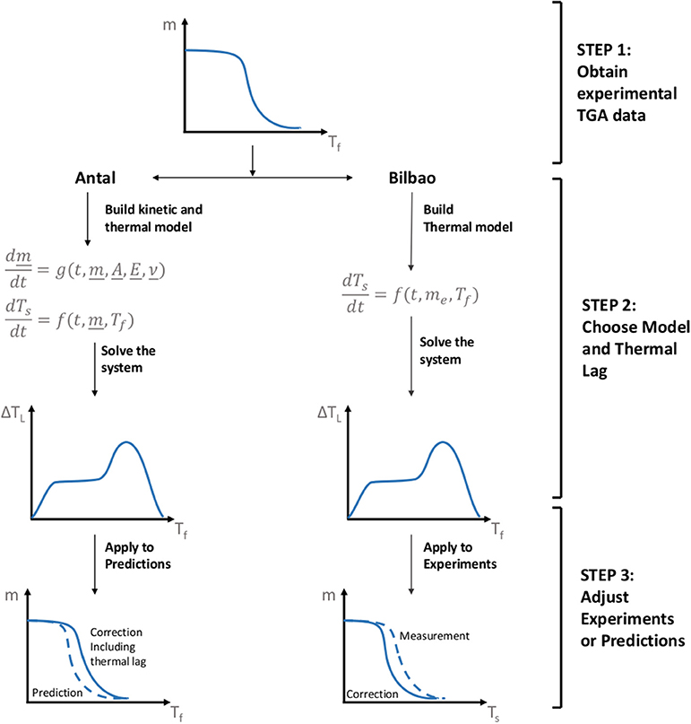
Figure 1. Overview of the two methodologies for estimating thermal lag in the literature. Both the method by Antal and Bilbao use an energy balance at the surface of the particle (assume lumped capacitance) as a thermal model, but Antal finds the source term from a kinetic model, while Bilbao finds the source term from a measurement.

The thermal model, in both methods, is an energy balance on the surface of the sample. Assuming the sample as an opaque, small, thermally thin spherical particle with surface area S in a large, open, heated environment yields (Equation 2)

$hS\left(T_f-T_s\right)+ϵ\sigma S\left(T_f^4-T_s^4\right)=m_{0}m\prime c\frac{d{T}_s}{dt}-m_0\frac{dm\prime }{dt}\Delta H(2)$

Where the left-hand side is the heat exchange with the environment. The first term on the right is the enthalpy change of the solid and the second term on the right is the enthalpy change due to the degradation of the solid (Atreya, 1998). Any released gas is assumed to be immediately transported away from the surface (Rein et al., 2006). The conservation of mass is expressed as in Richter and Rein (2017) and shown in simplified version in Equation (3).

$\begin{array}{rc}\frac{dm}{dt}=-mA{e}^{-E/R_u{T}_s}& (3)\end{array}$

Where m is the residual mass, A the pre-exponential factor, E the activation energy, and R_u is the universal gas constant. The reaction order is assumed to be one and the order of oxidation zero (pyrolysis reaction).

Rearranging Equation (2) gives Equation (4), which is in the same form as the conservation of mass.

$\begin{array}{rc}\frac{d{T}_s}{dt}=\frac{1}{m_{0}m\prime c}\left[hS(T_f-T_s)+ϵ\sigma S\left(T_f^4-T_s^4\right)+m_0\frac{dm\prime }{dt}\Delta H\right]& (4)\end{array}$

Assuming a shrinking spherical particle (Lin et al., 2012), we estimate the instantaneous surface area S and the convective heat transfer coefficient h as in Equations (5)–(7).

$\begin{array}{cc}R={\left(\frac{3}{4\pi }\frac{m_{0}m\prime }{\rho }\right)}^{1/3}& (5)\end{array}$

$S=4\pi R^2(6)$

$h=\frac{Nu{k}_f}{2R}\approx \frac{k_f}{R},assumingRe\to 0,soNu\to 2(7)$

In Equation (7) we assumed that the Nu → 2, which applies to a spherical particle moving with the flow (no relative velocity) (Hayhurst, 2013). It follows that Re → 0. Our estimation puts the Reynolds number (Re = UR/ν) at 2.4, based on flow velocity of 100 ml/min (Lin et al., 2009) in duct with a 12 mm diameter (Kislinger, 2016), a particle radius of R = 0.0013 m (~5 mg), and ν = 1.57 x 10⁻⁵ kg/m−s (Lemmon et al., 2016). This estimate supports the above assumption.

Method of Sensitivity Study

Here, we outline the procedure of the sensitivity study of the model formulations and the input parameters. The sensitivity of a thermal model was studied by comparing different formulations of the energy balance, which were coupled with the same kinetic model (Antal method). We compare five models labeled A to E. The first one, model A, is simulating just the mass loss, so that T_S = T_f. This case is the mode commonly found in the literature. The second one, model B, is the simulation of the surface temperature with a thermal model as given by Equations (4–7). The third one, model C, is model B with ϵ = 0. The fourth one, model D, is also model B, but with ϵ = 0 and assuming hS = 2.25 x 10⁻³ J s⁻² K (Lin et al., 2009) (just Equation 4). This last assumption represents a sphere of constant volume with diminishing density (Narayan and Antal, 1996). In the last one, model E, we use the kinetic and thermal model by Narayan and Antal (1996) as in Lin et al. (2009), where the kinetic model is expressed in mass conversion instead of residual mass. For all models we simulated the experiment of Lin et al. (2009) at 150 K/min to show the largest possible difference between the assumptions. The parameters for all simulations are given in Table 1.

TABLE 1

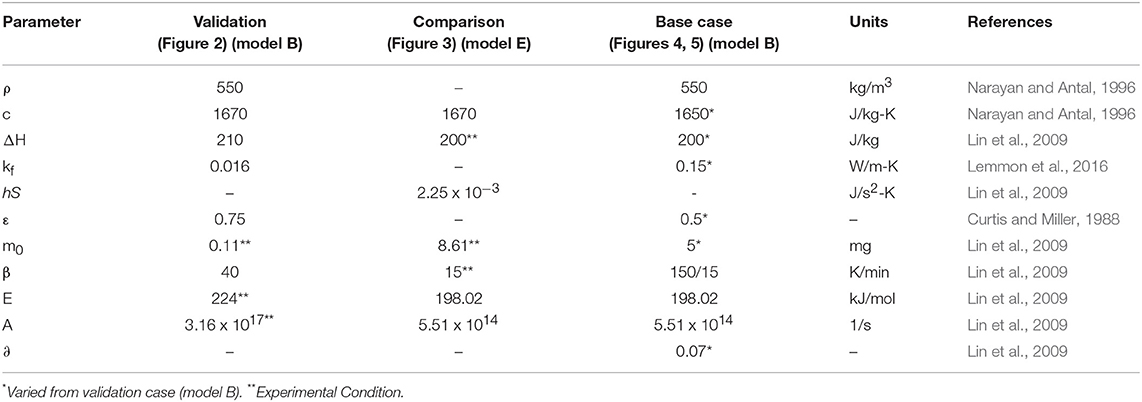
Table 1. Parameters for the validation and sensitivity study of the models.

A sensitivity coefficient was used to quantify the uncertainty due to the input parameters. The sensitivity coefficient for the maximum thermal lag is defined in Equation (8) (Wang and Sheen, 2015):

$s_j=\frac{\log \left(\Delta T_L^b\right)-log\left(\Delta T_L^m\right)}{\log \left(x_j^b\right)-log\left(x_j^m\right)}(8)$

Where $\Delta T_L^b$ is the maximum thermal lag in the base case, $\Delta T_L^m$ is the maxium thermal lag for the case with the modified parameter $x_j^m$, $x_j^b$ is the value in the base case for the jth parameter, and s_j is the sensitivity coefficient for the jth parameter. The parameters for the base case (model B) are reported in Table 1, and represent a typical experiment in a TGA. Each parameter was varied by ±25% and ±50% from its base value. The sensitivity coefficient reported here is the mean of these four simulations. Model B is used for the sensitivity study of the input parameters.

Selection of Input Parameters

This section describes the input parameters for each simulation in the subsequent sections of the paper. The validation was done with Model B and the parameters from Lin et al. (2009), fluid conductivity of nitrogen from Lemmon et al. (2016), and the initial and boundary conditions from Grønli et al. (1999). The analysis of the Antal and Bilbao method was done with Model E and the kinetic parameters, material properties, and experimental data from Lin et al. (2009). This formulation was chosen for consistency with the literature (Grønli et al., 1999; Lin et al., 2009). The density and the emissivity, not given by Lin et al, were taken from Narayan and Antal (1996) and Curtis and Miller (1988) respectively. The parameters of model B were modified from the validation case for the base case of the sensitivity study in order to vary them conveniently in their physical range. For all models, other than Model E, a char yield is required in the kinetic model. We estimated this missing char yield from the experiments by Lin et al. (2009).

Results

Comparison and Validation of Methods to Estimate Thermal Lag

Here, we validate and compare the three methods (Lin, Antal, Bilbao) to correct and estimate thermal lag in TGA experiments. Grønli et al. (1999) conducted three experiments to show the increase in thermal lag with sample mass using cellulose. To validate the Antal method, we corrected—by subtracting the thermal lag at each time step from the reported temperature (T_f) to obtain the surface temperature (T_s)–these measurements, as shown in Figure 2. All corrected measurements overlap—meaning that we eliminated thermal lag—so that we can judge the Antal method with our set of input parameters as valid for Avicel PH-101 cellulose.

FIGURE 2

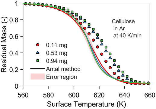
Figure 2. Validation of the Antal method using model B and a kinetic model expressed in mass conversion. The experiments and corresponding kinetic model are taken from Grønli et al. (1999). The material properties and heat of pyrolysis from Narayan and Antal (1996) (same author and cellulose as in the shown experiments). The shadow area represents the random error (2 K) in TGA. The symbols are the measurements by Grønli et al. (1999), and the lines are the corrected measurements using the Antal method.

To evaluate the difference between the Antal and Bilbao method we applied both methods to study the experiments of Lin et al. (2009). As shown in Figure 3, we compare the surface temperature, residual mass, mass loss rate, and thermal lag between the two methods at different heating rates. Figures 3A,D show that Antal's method predicts an earlier and lower thermal lag than Bilbao. Thermal lag is caused by the thermal inertia of the sample and the heat consumption of pyrolysis counteracted by the heat supply via convection and radiation. We had, therefore, expected the maximum thermal lag at the point of maximum heat consumption (peak mass loss rate in Figure 3C). The maximum thermal lag, however, occurs after the peak mass loss rate—roughly between 660 and 720 K—when the mass loss rate decayed. Cellulose has a sharp mass loss rate peak (around 650 K) at which the heat supply is small compared to the heat consumption. The thermal lag increases during this period (around 650 K), and only decreases when the mass loss rate decays (reduction in heat consumption). In other words, when the heat supply starts to becomes important again. Hence, the predicted peak thermal lag is delayed to the decay period of the mass loss rate, and higher for the Bilbao method, which predicts a longer decay (Figures 3B,C). The difference between the methods in magnitude (4 K) and position (20 K) is, however, small.

FIGURE 3

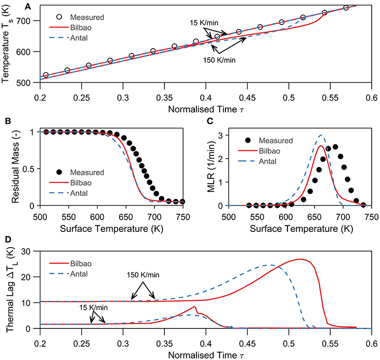
Figure 3. Comparison of the Antal (kinetic model) and Bilbao (no kinetic model) method using the thermal model E. All material properties, kinetic parameters, initial conditions, and boundary conditions are taken from Lin et al. (2009) for each shown simulation. (A) Comparison between measured (Lin et al., 2009) and corrected surface temperature by the Bilbao and Antal method of a cellulose particle at 15 and 150 K/min in helium. The normalized time is defined as τ = βt/(T_{t = ∞}−T₀). (B) Comparison between measured (Lin et al., 2009) and corrected residual mass–temperature history by the Bilbao and Antal method of a cellulose particle at 150 K/min in helium. (C) Comparison between measured (Lin et al., 2009) and corrected mass loss rate by the Bilbao and Antal method of a cellulose particle at 150 K/min in helium. (D) Comparison between calculated thermal lag by the Bilbao and Antal method of a cellulose particle at 15 K/min and 150 K/min in helium.

Lin et al. (2009) (Equation 1) also found a small difference between the Antal method and their own. Both methods yield the same kinetic parameters within 15% for the pre-exponential factor and 0.5 % for the activation energy. All three methods (Lin, Antal, Bilbao) yield, therefore, the same results. The method of Lin, however, is restricted to cellulose and similar polymers as it uses an empirical constant. Antal and Bilbao methods are instead valid generally by choosing the input parameters accordingly.

Uncertainty Quantification: Parameter Uncertainty vs. Model Uncertainty

In order to rigorously quantify the uncertainties of the predictions, we analyzed both the influence of model formulation and input parameters. Figure 4 presents the sensitivity study of the model formulation of the thermal model. It compares the different forms of the energy balance, model B to E, with the predicted residual mass, model A. Thermal lag (average: 16 K) is significant at this heating rate, but the exact formulation of the energy balance is not. All results (model B–E) adjusted with an energy equation lie closely together (Figure 4) with an average deviation of 2 K. This fact holds for both the residual mass and mass loss rate. For example, take model B and C that differ only by the radiation term. The maximum difference between the two is small (~5 K) compared to the actual thermal lag (~20 K). Hence, convection dominates the heat transfer, and the exact form of the energy equation is unimportant. Consequently, the uncertainty in the model assumptions (model uncertainty) is small.

FIGURE 4

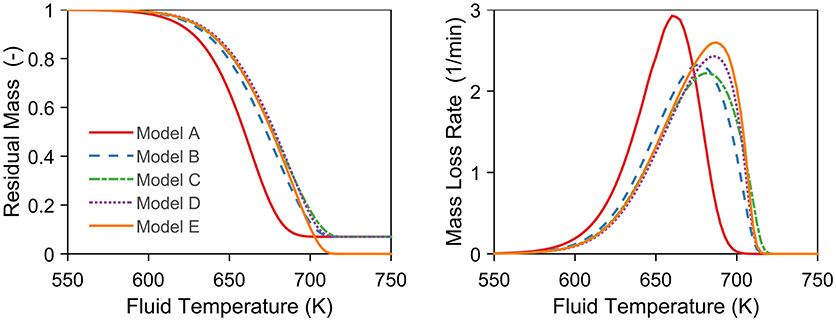
Figure 4. Sensitivity study of the model formulation of the thermal model. The simulations represent a 5 mg cellulose sample in inert atmosphere at 150 K/min. Model E has not been corrected with the final residual mass in this case.

Another source of uncertainty are the input parameters for which the sensitivity study is shown in Figure 5. Parameters which enhance thermal contact between the particle and fluid (k_f, ϵ) show a negative correlation with maximum thermal lag, as shown in Figure 5. On the other hand, parameters which reduce thermal contact, increase heat storage or consumption (m₀, ρ, c, ΔH) show a positive correlation with thermal lag. The most sensitive parameter, ΔH, is also the least known parameter for cellulose and biomass, varying by two orders of magnitude and the sign (endothermic or exothermic) (Roberts, 1971; Atreya and Baum, 2002; Anca-Couce, 2016). With a sensitivity factor of 0.84, this means that a thermal lag of 1 K could vary by 84 K which is significantly larger than the variation due to the choice of method (~20 K) or formulation (~5 K). It follows that uncertainty due to model formulation (model assumption) is small compared to the uncertainty in the input parameters. Bal and Rein (2013) previously discussed this trade-off between model and parameter uncertainty for polymers at the mesoscale (g-samples). Their discussion suggested that models should be kept simple (model D) until the uncertainty in the input parameters has been reduced. Further, it follows that one should only use the above methods to estimate uncertainties instead of correcting measurements, until the input parameter become more certain.

FIGURE 5

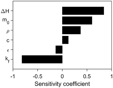
Figure 5. The sensitivity coefficient of the different input parameters of the thermal model. The coefficients were calculated from the maximum thermal lag at 15 K/min of the variation of the base case and have been averaged from four simulations (±25 and ±50%). The base case conditions and parameters are given in Table 1.

Discussion and Derivation of Thresholds

Intraparticle Heat Transfer

In order to study the intraparticle heat transfer, we derive a threshold of the sample mass below which temperature non-uniformities within the sample are negligible. We quantify the temperature uniformity within the sample by a temperature difference between the surface and center temperature (shown later). A temperature difference is a more convenient choice than a thermal gradient, as it allows us to define temperature uniformity independent of sample size. A negligible temperature gradient follows from a negligible temperature difference, and the two terms are used interchangeably.

We model the microscale sample as a particle. Let us write the heat-diffusion equation for an inert, solid cellulose particle—cellulose's heat of pyrolysis only reduces thermal differences (Appendix)—of outer radius R in perfect thermal contact with the surrounding fluid (h → ∞, Bi → ∞) as in Equation (9):

$\frac{\partial T}{\partial t}=\frac{\alpha }{r^2}\frac{\partial }{\partial r}\left(r^2\frac{\partial T}{\partial r}\right)(9)$

With the following boundary and initial conditions

$T\left(r,0\right)=T_{0}T\left(r=R,t\right)=T_s=T_0+\beta t(10)$

The Biot number (Bi = ∞) suggest significant thermal differences for all heating rates for this case. However, the analytical solution (Carslaw and Jaeger, 1959) to Equation (9) is Equation (11)

$\begin{array}{l}T\left(r,t\right)=T_0+\beta \left[t-\frac{R^2-r^2}{6\alpha }\right]\\ +\frac{2\beta R^3}{\alpha {\pi }^{3}r}{\displaystyle \sum _{n=1}^{\infty }\frac{{\left(-1\right)}^{n+1}}{n^3}{e}^{-n^2{\pi }^2\alpha t/R^2}\sin \frac{n\pi r}{R}}& (11)\end{array}$

As the surface of the particle is heated at a constant rate, we define in Equation (12) the temperature difference with respect to the surface temperature

$\Delta T_I\left(r,t\right)=T_s-T\left(r,t\right)(12)$

Now we can insert (Equations 10, 11) into (Equation 12) to obtain Equation (13)

$\begin{array}{l}\Delta T_I\left(r,t\right)=\beta \frac{R^2-r^2}{6\alpha }-\frac{2\beta R^3}{\alpha {\pi }^{3}r}\\ {\displaystyle \sum _{n=1}^{\infty }\frac{{\left(-1\right)}^{n+1}}{n^3}{e}^{-n^2{\pi }^2\alpha t/R^2}\sin \frac{n\pi r}{R}}& (13)\end{array}$

Examining Equation (13) reveals two things. Firstly, that the temperature difference is directly proportional to the ratio of heating rate and thermal diffusivity. Secondly, that there are two distinct terms one independent of, the first, and one depend on, the second, time. Hence, the evolution of ΔT_I is solely governed by the evolution of the second term. Closer inspection of this term reveals that its temporal behavior is governed by the exponential e^{−n2π2αt/R2}. As this term is negative, it follows from Equation (13) that ΔT_I is bounded by the following two extremes (Equations 14, 15)

$\Delta T_I\left(r,t\to 0\right)\to 0(14)$

$\Delta T_I\left(r,t\to \infty \right)\to \beta \frac{R^2-r^2}{6\alpha }(15)$

Consequently, thermal differences depend on the heating rate, which is not captured by the Biot number. From Equation (15) it follows that the maximum temperature difference occurs as t → ∞ and r → 0 and is given by Equation (16)

$\Delta T_I^{\infty }=\frac{\beta R^2}{6\alpha }(16)$

Therefore, the temperature difference reaches a steady state where it only depends on the radius, heating rate, and thermal diffusivity. For a 10 mg particle this state is reached within 10 s and for a 2 mg particle within 2 s (Appendix).

For comparison, Lyon (Lyon et al., 2012) and Melling (Melling et al., 1969) found a steady state of $\Delta T_I^{\infty }=\beta L^2/2\alpha$ and $\Delta T_I^{\infty }=\beta R^2/4\alpha$for a constantly heated slab and cylinder respectively. None of the above showed that the steady state also represents the maximum temperature difference.

Combining Equation (16) with Equation (5) yields the following expression (Equation 17) for thermal lag in terms of the initial sample mass:

$\Delta T_I^{\infty }=\frac{\beta {\left(\frac{3}{4\pi }\frac{m}{\rho }\right)}^{2/3}}{6\alpha }=C\beta m^{2/3}whereC=\frac{{\left(\frac{3}{4\pi \text{ρ}}\right)}^{2/3}}{6\alpha }(17)$

Let us define an upper bound or critical mass m_c below which thermal differences are small in terms of the maximum allowed temperature difference ($\Delta T_I^{\infty })$. We set the acceptable threshold as 1 K which could yield an error up to 5% in the kinetic parameters (Vyazovkin et al., 2011). Rearranging Equation (17) gives the critical mass in Equation (18).

$m_c={\left(\frac{\Delta T_I^{\infty }}{C\text{β}}\right)}^{3/2}(18)$

Figure 6 shows the dependence of the threshold on the heating rate. Our analysis is conservative as we have neglected internal heat consumption as well as assumed perfect thermal contact. In reality, h is finite which means that the heating rate experienced by the sample will be lower than recorded. Therefore, masses above the critical value might satisfy the criteria of a temperature difference below 1 K.

FIGURE 6

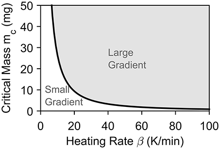
Figure 6. Shows the evolution of m_c against heating rate β for a maximum temperature difference of 1 K for a particle in perfect thermal contact with the surrounding (Bi = ∞). The area below the curve will experience insignificant thermal differences, while the area above the curve is likely to experience significant thermal differences.

Minimize Both Internal and External Heat Transfer Limitation

We can merge the results on inter- and intraparticle heat transfer through dimensional analysis as described in this section. For a sample to be kinetically controlled, the timescales of kinetics (τ_c), intraparticle heat transfer (τ_I), and interparticle heat transfer (τ_E) need to follow the order: τ_c > τ_E > τ_I. The maximum sample size can be estimated using the Biot and Damkohler number, which have to be below 0.1 (Prins et al., 2006; Hayhurst, 2013; Paulsen et al., 2013). Hayhurst (2013) found that the Biot number—ratio of intraparticle to interparticle heat transfer—is independent of the sample size as shown in Equation (19). The expression suggests to use a carrier gas of low k_f (Hayhurst, 2013). A lower k_f, however, also increases the Damkohler number, Equation (20). One can, therefore, only achieve kinetic-limited conditions if either the sample size is very small (Prins et al., 2006; Hayhurst, 2013; Paulsen et al., 2013) or the correct carrier gas is used. As shown in Figure 7, only a small number of carrier gases would be allowed even at low temperatures (340°C), when using dimensional analysis.

$Bi=\frac{{\tau }_I}{{\tau }_E}=\frac{0.3Nu{k}_f}{k_s}(19)$

$\begin{array}{ll}Da=\frac{{\tau }_E}{{\tau }_c}=\frac{2\rho c{R}^2\eta }{3k_f\text{Nu}}& (20)\end{array}$

This analysis applies only to isothermal conditions, while in non-isothermal conditions negligible temperature differences can be achieved even if Bi>0.1 (section Intraparticle Heat Transfer). Figure 8 shows the above analysis applied to non-isothermal experiments. The Biot number was replaced with our analytical threshold (solid blue line), (Equation 18), which shows good agreement with Lyon's threshold (gray dashed line) for intraparticle temperature differences (Lyon et al., 2012). Lyon's threshold is based on a sample of a synthetic polymer modeled as a slab with insignificant heat release, small thermal differences, and one-step kinetics. In comparison, our analysis is based on a particle of a natural polymer valid for all thermal differences and kinetics. Despite these difference, the thresholds agree closely because of the similar heat of reaction (Burnham et al., 2015) and kinetics between the two polymers.

FIGURE 7

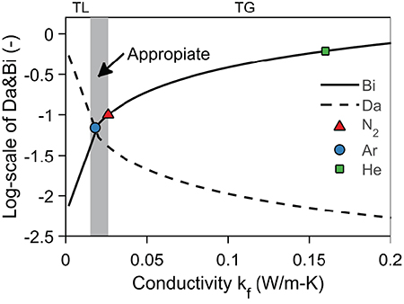
Figure 7. Illustrates the limited mechanism of heat transfer. TG stands for thermal differences and TL stands for thermal lag. The definition of the Bi and Da are given in Equations (19, 20). Kinetic parameters are taken from Lin et al. (2009), material properties from Narayan and Antal (1996) and fluid conductivities from Lemmon et al. (2016). The chemical time is taken at 340°C, upper limited of region where volatile production dominates (Bradbury et al., 1979). The length scale of the sample is taken as 560 μm (Paulsen et al., 2013) and the Nusselt number as 2.

FIGURE 8

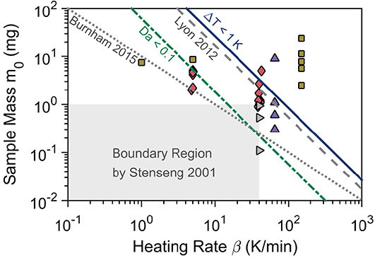
Figure 8. Summary of derived and literature thresholds for transport limitations together with high-quality experiments. The threshold by Burnham et al. (2015) (m_c = 10/β) is for both intra-and interparticle heat transfer. The threshold Da<0.1 (Equation 21) is for interparticle heat transfer with log T_s = 2.5 + 0.047 log β. The threshold by Lyon et al. (2012) ($m_c={(1.1/\beta )}^{3/2}$) and the threshold of ΔT_I < 1 K (Equation 18) are for intraparticle heat transfer. The experiments are by: Gronli et al. (diamonds) (Grønli et al., 1999), Gronli et al. (thermal lag study)(triangle right) (Grønli et al., 1999), Antal et al. (triangle up) (Antal et al., 1998), and Lin et al. (squares) (Lin et al., 2009). All boundaries and experiments, except Lyon, are for cellulose. The graph is inspired by Lyon et al. (2012) and Burnham (2017).

Figure 8 also reveals that interparticle heat transfer limits the maximum sample size, as the threshold of the Damkohler number (green dashed-dotted line) is below the intraparticle heat transfer threshold (blue solid line). To apply the Damkohler number to non-isothermal experiments we took the temperature of the peak mass loss rate as the characteristics temperature, and derived its dependence on the heating rate from experiments (Antal et al., 1998; Grønli et al., 1999).

Our Damkohler threshold (Equation 21) compares well with the threshold of Burnham et al. (2015) (gray dotted line) and Stenseng et al. (2001) (gray region) at the most common heating rates, 1 to 20 K/min. Deviations are only significant at very high or low heating rates. At low heating rates (below 10 K/min), the Damkohler number seems to overestimate the upper bound (critical) sample mass. Stenseng et al., however, proposed that larger sample mass (above 1 mg) can be employed at low heating rates. At high heating rates (above 10 K/min) the Damkohler number seems to underestimate the upper bound (critical) sample mass. Grønli et al. (1999) (triangle right) found thermal differences with sample masses down to 0.11 mg which agrees well with the Damkohler number threshold. Further Lin et al. (2009) (squares) found negligible thermal lag (less than 0.5 K) with roughly 5 mg at 1 K/min but significant thermal lag (5 K) at 15 K/min, which also agrees with the Damkohler number. The results from the round robin study by Grønli et al. (1999) at 5 K/min (diamonds) further support the validity of this threshold. Similar conclusions can be drawn for the intraparticle heat transfer threshold which is supported by Gronli et al. (diamonds) and Antal et al. (triangle up), where the experiment at 9 mg was conducted to show thermal limitations. Hence the thresholds derived here agree with the literature.

The results of Gronli et al. at 40 K/min (diamonds), Antal et al. (triangle up) at 65 K/min, and Lin et al. (squares) at 150 K/min seemingly disagree with our thresholds. However, our boundaries are conservative as we assume the sample to be a particle. Accurate kinetics can be achieved even with higher sample masses through careful experiments.

$\begin{array}{l}{m}_c=\frac{0.0775\pi }{\sqrt{\rho }}{\left(\frac{k_f\text{Nu}}{c\eta }\right)}^{3/2}\text{ with }\eta =Aexp\left(-\frac{E}{R{T}_s}\right)\text{with}\\ log{T}_s=2.5+0.047log\beta & (21)\end{array}$

We identified three main limitations of this study. Firstly, we only studied cellulose, which shows a sharper mass loss rate peak and a higher heat of pyrolysis compared to biomass. Thermal lag is therefore more severe in cellulose and our thresholds are conservative for biomass. This argument is supported by the experimentally obtained thresholds of 5 mg for wood (Anca-Couce et al., 2012) and 1 mg for cellulose (Stenseng et al., 2001). The close agreement between Lyon (synthetic polymer) and our (natural polymer) threshold also suggests that the above analysis holds for synthetic polymers. Further, Burnham (2017) found reasonable agreement when applying Lyons threshold to fossil fuels. Our results should, therefore, be applicable to all polymers with similar material properties, or with the input parameters adjusted accordingly as long as the dominate transport and heat consumption mechanisms are similar (e.g., no melting).

Secondly, we modeled the sample as a particle, which may lead to an incorrect sample length. Comparing measured (Paulsen et al., 2013) and predicted sample sizes, we found reasonable agreement (Figure 9). We overpredict the sample size by 23% which means that our results are conservative. Thirdly, we only focused on inert atmospheres. For natural polymers in reactive atmosphere the only difference is the oxidation of char which releases roughly 50 times the amount of heat per kg-fuel as the pyrolysis consumes (Anca-Couce et al., 2012). The yield of char for natural polymers is below 25%, which would give a heat of release of roughly 12.5 times the heat consumption during pyrolysis. Taking the constant of Lin et al. (0.131 min) (Lin et al., 2009), we get a thermal lag of 2 K in inert atmosphere and a thermal lead of 25 K in reactive atmosphere at 15 K/min. Hence, sample masses have to be significantly smaller in reactive atmosphere. Song et al. (2017) derived a threshold for the maximum sample size in air of roughly 10 mg based on the diffusion of oxygen—mass transfer effects in reactive environment—which is well-above the threshold for heat transfer. Their analysis supports our assumption that heat transfer is slower than mass transfer and, therefore, is the limiting mechanism in TGA.

FIGURE 9

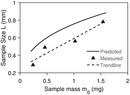
Figure 9. Comparison between predicted and measured length scale of sample in TGA. The measurements are from Paulsen et al. (2013).

The paper uses two definitions for the characteristic length in heat transfer. One, L₁, represents the smallest distance along the maximum temperature difference. For conduction in a spherical particle that is L₁ = R. The other, L₂, represents the average distance for heat conduction (volume divided by surface area). For a spherical particle $L_2=\frac{R}{3}$. The paper uses L₁ but also L₂ with regards to the previous work of Hayhurst (2013). L₁ is used in Equations (9–18) as well as Figures 6, 9. L₂ is used in Equations (19–21) as well as in Figures 7, 8.

Conclusion

In a TGA, samples should be sufficiently small for heat and mass transfer effects to be negligible. The aim of this study was to systematically analyse inter- and intraparticle heat transfer in TGA experiments, and to quantify the uncertainty in current methods to correct potential errors. We studied the first part by derive thresholds above which thermal lag and thermal gradients are significant. Our derived thresholds for intraparticle (Equation 18) and interparticle (Equation 21) heat transfer at the microscale compare well with the analytical and experimental thresholds from the literature up to 100 K/min. Comparing the intraparticle and interparticle threshold, we found that the sample size is always limited by interparticle heat transfer and has to be reduced with increasing heating rate and oxygen concentration. Our thresholds, however, are conservative, and larger sample masses could be used with careful verification.

Comparing three methods and their different formulations for correcting thermal lag in TGA experiments using uncertainty quantification methods, we found that the choice of method and formulation is negligible compared to the choice of input parameters. This fact stems from the large uncertainty in the input parameters compared to the uncertainty in the model formulation. As the input parameters are so uncertain, one should only use these methods to quantify uncertainties instead of correcting measurements of temperature in a TGA. Our results allow this quantification in published experiments, while our thresholds allow the design of appropriated future experiments. Comparison with the literature revealed that these results are valid for all natural polymers and likely for synthetics polymers as well. Hence, these results enable others to design or select appropriate TGA experiments, which will lead to a better understanding of the pyrolysis chemistry of polymers.

Author Contributions

FR and GR designed the research. FR carried out the research. FR and GR wrote the paper.

Funding

This work was financially supported by EPSRC (EP/M506345/1), Ove Arup, and the European Research Council (ERC) Consolidator Grant Haze (682587).

Conflict of Interest Statement

The authors declare that the research was conducted in the absence of any commercial or financial relationships that could be construed as a potential conflict of interest.

Acknowledgments

The authors would like to thank Dr Hafiz M. F. Amin and Matt Bonner from Imperial College London for their helpful comments.

References

Anca-Couce, A. (2016). Reaction mechanisms and multi-scale modelling of lignocellulosic biomass pyrolysis. Prog. Energy Combust. Sci. 53, 41–79. doi: 10.1016/j.pecs.2015.10.002

CrossRef Full Text | Google Scholar

Anca-Couce, A., Zobel, N., Berger, A., and Behrendt, F. (2012). Smouldering of pine wood: kinetics and reaction heats. Combust. Flame 159, 1708–1719. doi: 10.1016/j.combustflame.2011.11.015

CrossRef Full Text | Google Scholar

Antal, M. J., Varhegyi, G., and Jakab, E. (1998). Cellulose pyrolysis kinetics: revisited. Indus. Eng. Chem. Res. 37, 1267–1275. doi: 10.1021/ie970144v

CrossRef Full Text | Google Scholar

Atreya, A. (1998). Ignition of fires. Philos. Trans. R. Soc. Lond. A 356, 2787–2813. doi: 10.1098/rsta.1998.0298

CrossRef Full Text | Google Scholar

Atreya, A., and Baum, H. R. (2002). A model of opposed-flow flame spread over charring materials. Proc. Combust. Inst. 29, 227–236. doi: 10.1016/S1540-7489(02)80031-1

CrossRef Full Text | Google Scholar

Bal, N., and Rein, G. (2013). Relevant model complexity for non-charring polymer pyrolysis. Fire Safety J. 61, 36–44. doi: 10.1016/j.firesaf.2013.08.015

CrossRef Full Text | Google Scholar

Bilbao, R., Arauzo, J., and Millera, A. (1987). Kinetics of thermal decomposition of cellulose. Part II. Temperature differences between gas and solid at high heating rates. Thermochim. Acta 120, 133–141. doi: 10.1016/0040-6031(87)80212-5

CrossRef Full Text | Google Scholar

Bilbao, R., Murillo, M. B., Millera, A., and Mastral, J. F. (1991). Thermal decomposition of lignocellulosic materials : comparison of the results obtained in different experimental systems Thermochim. Acta 190, 163–173.

Google Scholar

Bradbury, A. G. W., Sakai, Y., and Shafizadeh, F. (1979). A kinetic model for pyrolysis of cellulose. J. Appl. Polym. Sci. 23, 3271–3280. doi: 10.1002/app.1979.070231112

CrossRef Full Text | Google Scholar

Burnham, A. K. (2017). Global Chemical Kinetics of Fossil Fuels. Cham: Springer International Publishing. doi: 10.1007/978-3-319-49634-4

CrossRef Full Text | Google Scholar

Burnham, A. K., Zhou, X., and Broadbelt, L. J. (2015). Critical review of the global chemical kinetics of cellulose thermal decomposition. Energy Fuels 29, 2906–2918. doi: 10.1021/acs.energyfuels.5b00350

CrossRef Full Text | Google Scholar

Carslaw, H. S., and Jaeger, J. C. (1959). Conduction of Heat in Solids, 2nd Edn. Oxford: Clarendon Press.

Chan, W.-C. R., Kelbon, M., and Krieger, B. B. (1985). Modelling and experimental verification of physical and chemical processes during pyrolysis of a large biomass particle. Fuel 64, 1505–1513. doi: 10.1016/0016-2361(85)90364-3

CrossRef Full Text | Google Scholar

Curtis, L. J., and Miller, D. J. (1988). Transport model with radiative heat transfer for rapid cellulose pyrolysis. Indus. Eng. Chem. Res. 27, 1775–1783. doi: 10.1021/ie00082a007

CrossRef Full Text | Google Scholar

Grønli, M., J., Antal, M., and Várhegyi, G. (1999). A round-robin study of cellulose pyrolysis kinetics by thermogravimetry. Indus. Eng. Chem. Res. 38, 2238–2244. doi: 10.1021/ie980601n

CrossRef Full Text | Google Scholar

Hayhurst, A. N. (2013). The kinetics of the pyrolysis or devolatilisation of sewage sludge and other solid fuels. Combust. Flame 160, 138–144. doi: 10.1016/j.combustflame.2012.09.003

CrossRef Full Text | Google Scholar

Kislinger, J. (2016). E-mail exchange about dimensions of a Mettler Toledo TGA furnance, Personal Communication.

Lédé, J., and Authier, O. (2015). Temperature and heating rate of solid particles undergoing a thermal decomposition. which criteria for characterizing fast pyrolysis? J. Anal. Appl. Pyrol. 113, 1–14. doi: 10.1016/j.jaap.2014.11.013

CrossRef Full Text | Google Scholar

Lemmon, E. W., McLinden, M. O., and Friend, D. G. (2016). “Thermophysical properties of fluid systems,” in NIST Chemistry WebBook, NIST Standard Reference Database Number 69, eds W. G. Linstrom and P.J. Mallard (Gaithersburg, MD: National Institute of Standards and Technology). Available online at: http://webbook.nist.gov (Accessed June 10).

Google Scholar

Lin, Y., Cho, J., Davis, J. M., and Huber, G. W. (2012). Reaction-transport model for the pyrolysis of shrinking cellulose particles. Chem. Eng. Sci. 74, 160–171. doi: 10.1016/j.ces.2012.02.016

CrossRef Full Text | Google Scholar

Lin, Y.-C., Cho, J., Tompsett, G. A., Westmoreland, P. R., and Huber, G. W. (2009). Kinetics and mechanism of cellulose pyrolysis. J. Phys. Chem. C 113, 20097–20107. doi: 10.1021/jp906702p

CrossRef Full Text | Google Scholar

Lyon, R. E., Safronava, N., Senese, J., and Stoliarov, S. I. (2012). Thermokinetic model of sample response in nonisothermal analysis. Thermochim. Acta 545, 82–89. doi: 10.1016/j.tca.2012.06.034

CrossRef Full Text | Google Scholar

Melling, R., Wilburn, F. W., and McIntosh, R. M. (1969). Study of thermal effects observed by differential thermal analysis. Theory and its application to influence of sample parameters on a typical DTA curve. Anal. Chem. 41, 1275–1286. doi: 10.1021/ac60279a009

CrossRef Full Text | Google Scholar

Narayan, R., and Antal, M. J. (1996). Thermal lag, fusion, and the compensation effect during biomass pyrolysis. Indus. Eng. Chem. Res. 35, 1711–1721. doi: 10.1021/ie950368i

CrossRef Full Text | Google Scholar

Paulsen, A. D., Mettler, M. S., and Dauenhauer, P. J. (2013). The role of sample dimension and temperature in cellulose pyrolysis. Energy Fuels 27, 2126–2134. doi: 10.1021/ef302117j

CrossRef Full Text | Google Scholar

Prins, M. J., Ptasinski, K. J., and Janssen, F. J. J. G. (2006). Torrefaction of wood. Part 1. Weight loss kinetics. J.Anal. Appl. Pyrol. 77, 28–34. doi: 10.1016/j.jaap.2006.01.002

CrossRef Full Text | Google Scholar

Ranzi, E., Faravelli, T., and Manenti, F. (2016). Chapter one – Pyrolysis, gasification, and combustion of solid fuels. Adv. Chem. Eng. 49, 1–94. doi: 10.1016/bs.ache.2016.09.001

CrossRef Full Text | Google Scholar

Rein, G. (2008). From pyrolysis kinetics to models of condense-phase burning. Revent Adv. Flame Retard. Polym. Mater. 19, 1–10.

Rein, G., Lautenberger, C. W., Fernandez-Pello, A. C., Torero, J. L., and Urban, D. L. (2006). Application of genetic algorithms and thermogravimetry to determine the kinetics of polyurethane foam in smoldering combustion. Combust. Flame 146, 95–108. doi: 10.1016/j.combustflame.2006.04.013

CrossRef Full Text | Google Scholar

Richter, F., and Rein, G. (2017). Pyrolysis kinetics and multi-objective inverse modelling of cellulose at the microscale. Fire Safety J. 91, 191–199. doi: 10.1016/j.firesaf.2017.03.082

CrossRef Full Text | Google Scholar

Roberts, A. F. (1971). The heat of reaction during the pyrolysis of wood. Combust. Flame 17, 79–86. doi: 10.1016/S0010-2180(71)80141-4

CrossRef Full Text | Google Scholar

Song, Z., Huang, X., Luo, M., Gong, J., and Pan, X. (2017). Experimental study on the diffusion–kinetics interaction in heterogeneous reaction of coal. J. Thermal Anal. Calorimetry 129, 1625–1637. doi: 10.1007/s10973-017-6386-1

CrossRef Full Text | Google Scholar

Stenseng, M., Jensen, A., and Dam-Johansen, K. (2001). Investigation of biomass pyrolysis by thermogravimetric analysis and differential scanning calorimetry. J. Anal. Appl. Pyrol. 58, 765–780. doi: 10.1016/s0165-2370(00)00200-x

CrossRef Full Text | Google Scholar

Vyazovkin, S., Burnham, A. K., Criado, J. M., Pérez-Maqueda, L. A., Popescu, C., and Sbirrazzuoli, N. (2011). ICTAC kinetics committee recommendations for performing kinetic computations on thermal analysis data. Thermochim. Acta 520, 1–19. doi: 10.1016/j.tca.2011.03.034

CrossRef Full Text | Google Scholar

Wang, H., and Sheen, D. A. (2015). Combustion kinetic model uncertainty quantification, propagation and minimization. Prog. Energy Combust. Sci. 47, 1–31. doi: 10.1016/j.pecs.2014.10.002

CrossRef Full Text | Google Scholar

Appendix

Reduction of Temperature Difference With an Endothermic Reaction

Cellulose pyrolysis is net endothermic (heat consumption), meaning that the reaction tends to cool the sample (Curtis and Miller, 1988). This effect is particularly strong in high temperature regions, where the reaction rate is also high. This argument is supported by the analysis below.

Let us assume a parabolic temperature profile in the particle

$T\propto r^2(\text{A}1)$

Let us now assume that the heat consumed is proportional to the reacting mass and that the rate constant is proportional to the temperature

$Q\propto \eta m(\text{A}2)$

$Q\propto \eta \rho S\delta (\text{A}3)$

$Q\propto \eta r^2(\text{A}4)$

$Q\propto r^4(\text{A}5)$

We can then write the temperature at each radius as

$T(r,t)T_{r=0}+C_1{r}^2(\text{A}6)$

and the reduction in temperature due to heat consumption at each radius as

$Q=C_2{r}^4(\text{A}7)$

Now we obtain the temperature difference, using Equations (27, 28), as

$\begin{array}{ll}\Delta T_I(r)\approx T_s-(T(r,t)-Q)& (\text{A}8)\end{array}$

$\begin{array}{ll}=T_s-(T_{r=0}+C_1{r}^2-C_2{r}^4)& (\text{A}9)\end{array}$

$\begin{array}{ll}=C_1\left(R^2-r^2\right)-C_2(R^4-r^4)& (\text{A}10)\end{array}$

Two things are evident from this analysis. Firstly, the temperature difference now contains two terms: one, the first, for thermal inertia and one, the second, for the chemical reaction. Secondly, the maximum temperature difference occurs when r = 0 and C₂ = 0. This highly simplified analysis confirms that heat consumption decreases the temperature difference inside the solid.

Rate of Convergence

Let us denote the steady state term, the first, by θ_s and the transient term, the second, by θ_t in Equation (12). We want to know when θ_t is neglectable with respect to θ_s. Therefore, we compare the evolution of the transient term divided by the steady state term, as shown below, and illustrated in Figure A1.

$\frac{{\theta }_t}{{\theta }_s}=\frac{12}{\frac{{\pi }^{3}r}{R}(1-r^2/R^2)}{\displaystyle \sum _{n=1}^{\infty }\frac{{\left(-1\right)}^{n+1}}{n^3}}{e}^{-}{n}^2{\pi }^2\alpha t/R^2\sin \frac{n\pi r}{R}(\text{A}11)$

The infinite series was solved for the first 5,000 terms and rapidly convergences to zero. Within 10 s it is negligible. The rate of convergence increases with decreasing sample mass as m → 0 which implies R → 0. Then the Fourier number (αt/R²) goes to infinity independent of the value of t, from which follows that θ_t → 0.

FIGURE A1

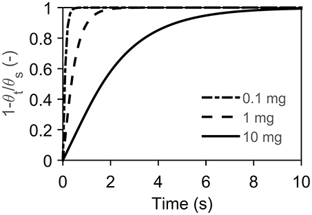
Figure A1. Shows the rate of convergence (independent of heating rate) for several mass at r/R = 0.1 due to the singularity at r/R = 0. The material properties are from Narayan and Antal (1996).

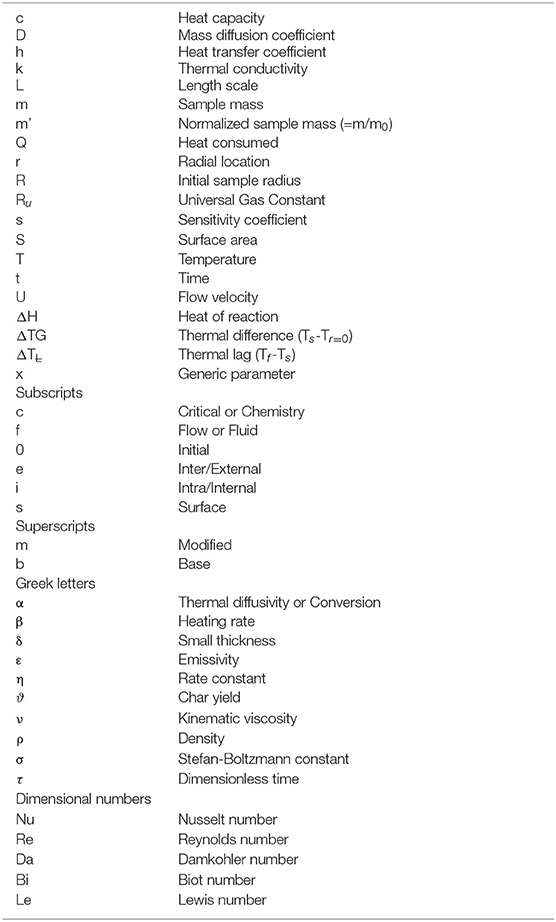
Nomenclature