Modeling Wind Direction Distributions Using a Diagnostic Model in the Context of Probabilistic Fire Spread Prediction

1. Introduction

The accurate prediction of wind fields across all types of terrain is fundamental to capturing the range of possible spreading patterns a fire can exhibit. Operational wind and fire spread models are typically deterministic; a single collection of input variables gives rise to a single and fixed prediction value. However, wind fields and fire spread are driven by a range of processes which can experience variations at multiple scales, some of which cannot be fully captured within operationally constrained models. This gives rise to uncertainty in predicted fire behaviors. To address this uncertainty, probabilistic modeling techniques have emerged in the field of fire prediction.

Newly developed fire modeling frameworks allow for the prediction of fire perimeters and characteristics with associated probabilities, resulting in scenarios being analyzed in the context of risk and likelihood. Cruz (2010) noted that ensemble predictions would extend the interpretation of predicted outcomes, not necessarily improving individual prediction accuracy but providing more information to model end users. Even in early fire modeling research, Kourtz (1972) indicated potential improvements in the reliability of predictions by using such techniques. More recently, it was demonstrated that the ensemble-based decision support tool, FireDST, was able to produce a probabilistic prediction that adequately covered the actual extent of an observed fire, as such implying that it is plausible to view the actual fire as a realization of the ensemble distribution. This approach allowed for the provision of detailed probabilistic information about exposure and potential losses (French et al., 2013). Such information could be scrutinized by emergency service managers to analyze the variety of potential outcomes and impacts from a single event.

To construct probabilistic predictions, frameworks such as SABRE (Twomey and Sturgess, 2016) and FireDST (French et al., 2013, 2014) developed in Australia, and FSPro (Finney et al., 2011) developing in the US, have considered such ensemble-based probabilistic approaches to fire modeling through variations of the input parameters using pre-determined distribution structures. Probabilistic prediction of terrain-modified wind fields is therefore vital to the accurate and informative modeling of fire spread as a key model input but also as a tool for identifying the varying likelihood of important fire behaviors, which can arise as a consequence of complex wind-terrain interaction (e.g., Sharples et al., 2012). The information gleaned from probabilistic wind models can also help identify parts of the landscape where three-way interactions between the wind, the terrain and a fire can dominate fire propagation; these are instances where coupled fire-atmosphere models may be required to overcome the limitations of traditional surface-based fire spread models.

However, the distribution structures used in current operational fire prediction, such as the Uniform, Gaussian or point distributions, may not be most representative of the true variability of factors driving surface fire behavior. In the context of fire spread prediction, wind fields have been considered in probabilistic terms in only a limited number of studies (e.g., Sharples et al., 2010). In contrast, the wind energy and environmental sciences sectors have contributed analyses that consistently show the variability of wind speed and direction to be more complex, exhibiting features such as skewness, multi-modality and non-stationarity (e.g., Carta et al., 2008a,b; Erdem and Shi, 2011; Alegría et al., 2016; Lagona and Picone, 2016). In addition, Quill (2017) highlighted that the structure of wind direction distributions can vary considerably through space.

For effective modeling of bushfire spread across complex landscapes, input variables need to be modeled at all relevant scales. Mesoscale Numerical Weather Prediction (NWP) systems provide accurate real-time weather predictions over a range of appropriate spatio-temporal scales but, with horizontal resolutions from 3km up to 12km, these models do not resolve winds at sufficient scales to capture detailed topographic effects that can influence surface fire behavior. In particular, Wagenbrenner et al. (2016) highlighted the limited ability of broad-scale weather prediction to capture the variability of wind fields across complex terrain and indicated the need for downscaling models to better predict meteorological variables at finer resolutions.

WindNinja is the primary down-scaling wind model for bushfire prediction across numerous countries, including Australia, Greece, Canada and the United States (Forthofer et al., 2014a). In particular, WindNinja is operationally applied within the Phoenix Rapidfire model utilized across Eastern Australia (Tolhurst et al., 2008), as well as within FARSITE, Behave and FlamMap, among others, which are routinely used across the US¹. WindNinja was originally developed due to a lack of operational down-scaling wind models available or widely used for bush-fire prediction (Forthofer, 2007) and, due to its success, few alternatives have been developed. As a deterministic diagnostic model, WindNinja is generally preferred for operations, as opposed to prognostic approaches using full computational fluid dynamics (CFD) models, due to the computational constraints on producing useful, fine-scale wind model outputs in real or near-real time (Forthofer et al., 2014b). It has also been shown that full physical wind models can be highly sensitive to input data such as surface roughness or boundary layer conditions over complex terrain, where these details are often not available in operational contexts (Lopes, 2003). However, due to the simplification of physical equations needed to obtain this computational efficiency, WindNinja is known to have significant limitations.

A number of evaluation studies throughout the development of the WindNinja software have compared the mass-consistent model to wind observations taken over complex terrain (Forthofer et al., 2014b; Butler et al., 2015; Wagenbrenner et al., 2016), as well as comparing fire spread prediction driven by the WindNinja model to those driven by a full CFD wind model (Forthofer et al., 2014a). Each of these studies has highlighted the greatest limitations of the model on leeward slopes where the complex nature of the flow field, including separation, can cause unsteady flow. It was noted by Wagenbrenner et al. (2016) that they were in fact to be expected since the version WindNinja 2.5.2 was designed to account for only mass-conservation across the landscape and did not take into consideration momentum conservation which causes features such as re-circulation on leeward slopes. Some of these issues were resolved by the addition of a momentum solver in later versions of the model (to be published), yet it is expected to have similar limitations on leeward slopes as seen by Forthofer et al. (2014b).

The limitations of models such as WindNinja are well documented and well understood. Forthofer et al. (2014b) warned that users should be aware of model limitations and interpret results cautiously where appropriate. The potential consequences of not capturing particular wind features in the context of fire modeling are significant, with characteristics such as flow separation on leeward slopes linked to extreme fire behaviors (Sharples et al., 2012; Simpson et al., 2013). However, the known limitations of deterministic wind field predictions have yet to be rigorously characterized for the purposes of quantifying error propagation or uncertainty in operational fire modeling.

In an investigation into the uncertainty of fire spread predictions, Cruz and Alexander (2013) suggested that, across the current global suite of fire models, percentage errors in the rates of spread predictions range from 20% up to 40%. The authors went as far as to say that “one could argue that perhaps the only certainty about wild-land fire behavior prediction is that it is extremely unlikely that a prediction will match the observed fire behavior characteristics” (Cruz and Alexander, 2013, p. 20). The main sources of uncertainty in fire rates of spread prediction have been cited as a lack of model applicability, internal model inaccuracy and input data errors (Albini, 1976; Alexander and Cruz, 2013). Operational settings have also been suggested to increase potential errors, particularly for data inputs, with greater uncertainty in weather forecasts and fuel variability (Cruz and Alexander, 2013).

There is currently limited literature quantifying uncertainty in operational fire prediction frameworks. Cruz (2010) noted that gaps in dealing with uncertainty exist in both literature and operations, and commented, for example, that the lack of confidence intervals for deterministic predictions leaves the onus of uncertainty estimation solely with the decision makers. Sensitivity analyses are one way to better understand the propagation of errors through a modeling framework and their impacts on final predicted outputs. One analysis of Phoenix Rapidfire, used in the Australian environment, was conducted by Penman et al. (2013) and concluded that fire weather (as characterized by the McArthur Forest Fire Danger Index) had the greatest influence on fire behavior, over suppression efforts and fuel treatments. The Forest Fire Danger Index (FFDI) is a function of temperature, relative humidity, wind speed, fuel moisture and fuel availability (Noble et al., 1980) and is classified into five categories. Penman et al. (2013) considered the sensitivity of fire outcomes in terms of these five categories, finding that increased FFDI led to reduced probability of containment, increased fire size and increased distance traveled by the fire. However, as far as the authors are aware, no detailed analysis of the influence of individual input parameters, such as wind speed, has been conducted. Although beyond the scope of this study, this research looks to drive toward such analysis.

The focus of this research is to consider wind direction, conditioned on wind speed, as an input variable to fire prediction. Clear links have been shown between wind speed and fire behavior through the traditional fire spread prediction models using tools such as the FFDI with broad-scale wind direction assumed to be the key driver of fire spread direction (Noble et al., 1980). Yet new research into extreme fires suggests that terrain-level wind direction can have significant impacts on fire behavior, including the generation of vorticity-driven lateral spread which can see fire propagate in directions perpendicular to the prevailing wind (Simpson et al., 2013). However, such behaviors are yet to be captured in traditional fire models.

Leading from the emergence of work in fire modeling, to better understand bushfire prediction uncertainty with the use of ensemble or stochastic modeling, this research reframes wind prediction in probabilistic terms. The study then aims to understand the capacity of the operational deterministic wind model WindNinja to capture terrain-level variability of wind fields. A novel application of the existing model is taken to predict the distribution of wind directions observed over complex terrain. By recasting wind fields in terms of probability distributions, the limitations of current modeling techniques can be quantified. Accurately modeled probability distributions of wind characteristics can feed directly into the ensemble-based fire modeling frameworks that are currently operational in Australia but require further uncertainty analysis. While this analysis remains beyond the scope of the present study, it is an important area of further research in the field and will help facilitate more informed decision making.

The remaining sections are organized as follows. Section 2 details the data collected and analyzed for this research, including the framing of wind direction distributions. Section 3 outlines the deterministic wind model WindNinja, using both mass-consistent and mass-and-momentum consistent solvers, as well as detailing the novel application of the model to predict wind direction distributions. Section 4 describes the comparison of wind model outputs with observed wind direction distributions, followed by a discussion of the results in section 5. Finally, section 6 concludes the study.

2. Observed Data

2.1. Case Study Region

Wind observations were taken across Flea Creek Valley (FCV) in the Brindabella National Park, approximately 40 km west of Canberra, Australia (Figure 1) (Quill and Sharples, 2018). The terrain across the broader region can be classified as rugged (McRae and Sharples, 2013), with elevation across the study area ranging from 767 m up to 1,077 m. The study area is dominated by Eucalyptus forest, with canopies up to approximately 15 m. The valley was heavily affected by fire in 2003, when atypical fire spread was observed in the region (McRae, 2004; Sharples et al., 2010).

FIGURE 1

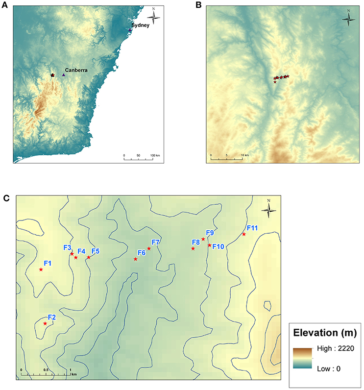
Figure 1. Maps showing the locations of weather station sites. (A) Shows south-eastern Australia, (B) shows the broad topography surrounding the study region, and (C) shows the location of the eleven weather stations F1–F11 across Flea Creek Valley.

The Bureau of Meteorology (BoM) have permanent automatic weather stations situated at Mount Ginini (approximately 20 km south) and Canberra Airport (approximately 40 km east) which reflect the broad scale meteorology experienced across the region. The synoptic patterns in the region are dominated by high-pressure weather systems which produce west-northwesterly (WNW) winds during the summer and westerly winds throughout the winter. Flea Creek Valley runs approximately North-South through the Brindabella Ranges, and so is aligned approximately perpendicularly to the dominant WNW prevailing wind direction.

Eleven Davis^® Vantage Pro 2 portable automatic weather stations with Weatherlink^® data loggers connected to Raspberry Pi^® microcomputers were used to collect data across Flea Creek Valley. The stations were set approximately 300–500 m apart along a 3–4 km East-West transect of the valley. The locations of the stations (F1 to F11) are indicated in Figure 1, and Table 1 outlines the vegetation and topographic details of each site. Topography was obtained through ArcGIS (ESRI, 2011) analysis of the SRTM 90m Digital Elevation Model.

TABLE 1

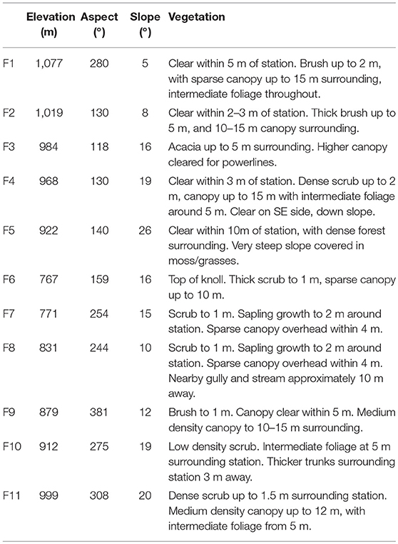
Table 1. Topographic and vegetation details for each site across Flea Creek Valley.

Each station recorded wind speed and wind direction at 5 meters above ground level using horizontal cup anemometers and wind vanes. Wind speeds were recorded at an accuracy of 0.4 ms⁻¹, while wind directions were recorded in 22.5° bins, corresponding to the 16 points of the compass. Data associated with very low wind speeds (below 0.4 ms⁻¹) were excluded from analysis. Data were collected at 1-min intervals from 10th July to 15th December 2014. With a station sampling frequency of 3 s, wind direction observations were recorded as the dominant wind direction sampled over 1 min, while wind speed observations were the average of wind speeds sampled over the minute. Table 2 details the number of non-zero observations taken for each wind characteristic (speed and direction) over the study period at each site across FCV.

TABLE 2

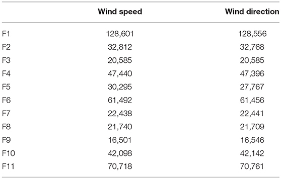
Table 2. Summary of sample sizes for observed non-zero (≥ 0.4 ms⁻¹) wind characteristics across Flea Creek Valley.

Wind data at these spatial and temporal resolutions, collected with these equipment, are limited to two-dimensional analysis of wind fields at the terrain scale. Although finer resolution three-dimensional data would allow more detailed analysis of fine-scale wind field movements, including the effects of the canopy and turbulence behavior, these are not within the scope of this study. The coarser resolution of this dataset allows for useful insights into terrain-level wind fields, at spatial resolutions akin to those predicted by operational down-scaling models like WindNinja, i.e., 90 m spatial resolutions (which are limited by availability of topography data) for real-time fire modeling at, say, 10-min intervals. An analysis, shown in later sections, also highlights consistent wind behaviors captured by this dataset, providing useful meteorological insights.

At 5 m above ground, the anemometers were located within the vegetation canopy, with efforts made to ensure stations were not directly impeded by vegetation, within a few meters (Table 1). Modeled wind fields were predicted at 5 m above the canopy and so cannot be directly compared due to the well-known effects of canopies on wind fields (e.g., Finnigan, 2000; Finnigan and Belcher, 2006; Belcher et al., 2012). In application to bushfire modeling, predicted wind speeds from above the canopy are transformed to within-canopy winds using wind reduction factors (Andrews, 2012; Quill et al., 2016; Moon et al., 2019). However, predicted wind directions undergo no such transformation. Therefore, in the context of bushfire prediction, wind directions modeled at 5 m above the canopy are equivalent to wind directions predicted within the canopy and, on this basis, are compared to those observed for this study.

Observed within-canopy wind directions across Flea Creek Valley show consistent behaviors across the study period, suggesting that winds beneath the canopy are structured in relation to the prevailing winds above the canopy, rather than dominated by canopy effects. Such wind field structures are important to the driving of fires beneath and within canopies and quantifying such behaviors (where they are not well modeled) is an important step in understanding uncertainty propagation in surface fire prediction.

2.2. Wind Observations

Figure 2 summarizes the winds observed over the collection period at each site across FCV. Wind data collected from the ridge top stations on both the western and eastern sides of the valley (F1, F2, and F11) indicate the most frequently observed westerly to north-westerly prevailing wind direction. Less frequent easterly prevailing winds were also observed at F1. On the western slopes of the valley (F3 and F4), the dominant easterly wind direction indicates the prevalence of wind reversals when these slopes were leeward to the westerly prevailing winds. At F5, on this western slope, south-westerly winds are experienced most frequently. The site is located on a steep south-facing slope and winds are likely impacted by mechanical or thermal flows driven by this sheer topography.

FIGURE 2

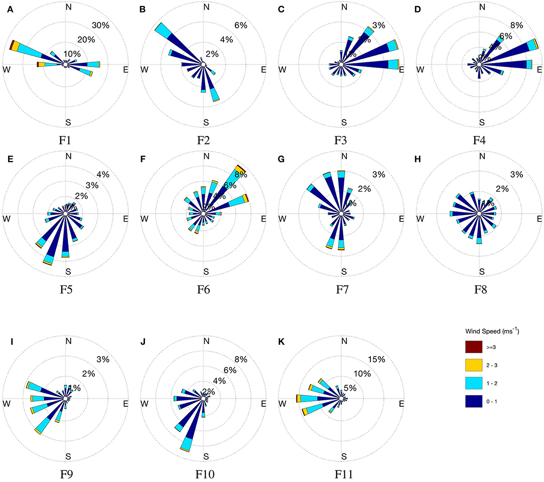
Figure 2. Observed wind roses for each site (A–K) F1 to F11, across Flea Creek Valley.

On the valley floor (F6 and F7), northerly and southerly modes (northeast and southwest at F6) suggest that channeling along the valley axis may have dominated wind movement through this region. On the eastern slope at F8, the wind speeds are very low, leading to considerable variability in wind direction. Finally, on the eastern slope (F9 and F10), south-westerly observations indicate a southerly bias in the winds, most often observed when this slope was windward to the WNW prevailing winds. Local topographical features such as small-scale gullies running up the side of Flea Creek Valley (see contours in Figure 1C) may also cause a deviation from the prevailing wind direction.

To better understand the drivers behind observed wind behaviors at each site, Figure 3 shows the average hourly wind speed and the average hourly wind direction at times which exemplify diurnal patterns, i.e., 03000 h, 0900 h, 1500 h, and 2100 h. Unfortunately, taking the mean of bimodal distributions such as those observed at F1, F2, and F7 can cause issues with such analysis. For instance, the northerly wind direction shown at F1 at 0900 h and 2100 h is not strongly indicated in Figure 2. These are in fact a result of significant intra-hourly west to north-westerlies despite more prominent easterlies over-night. Similarly, the south-western ridge top station at F2 shows SW winds in Figure 3, which result from averaging the NW and SE modes indicated in Figure 2. These intra-hour variations suggest no strong diurnal patterns, with mechanical forcing a more likely explanation for the bimodal wind directions.

FIGURE 3

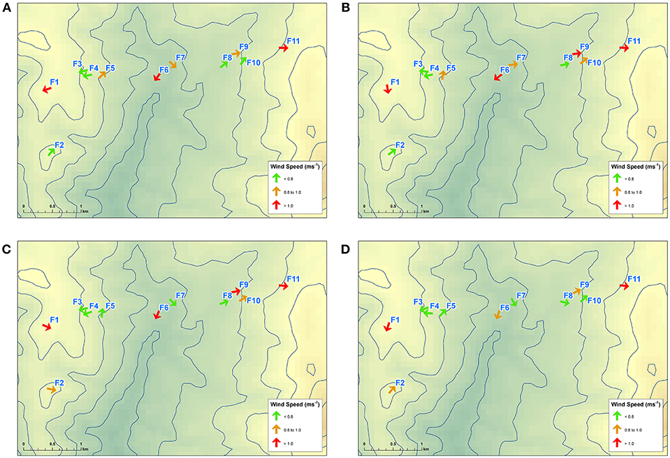
Figure 3. Observed average hourly wind directions at each site across Flea Creek Valley, at (A) 0300 h, (B) 0900 h, (C) 1500 h, and (D) 2100 h.

Despite the northerly bias, average hourly wind directions at the north-western ridge top station (F1) rotated from NE over-night (0300 h) through to NW in the afternoon (1500 h). The easterly shift in wind direction at F1 was echoed by a similar regional wind direction change observed at Canberra Airport, and was coupled with an increase in wind speed across the valley. The higher afternoon wind speeds were predominantly felt along the valley floor and on the west-facing (or windward) slope. The leeward slope winds remained relatively low during the afternoon period.

Despite the change in wind direction observed at F1, the remaining stations showed stable wind directions throughout Figure 3, corresponding to the unimodal distributions shown in Figure 2. Each other station experienced consistent wind directions throughout the night and day, suggesting that diurnal effects had little impact on wind flow beneath the canopy across the valley. Most prominently on the valley floor at F6, northerly average flows agreed with the dominant northerly and north-easterly modes shown in Figure 2. The average northerlies were experienced throughout the day and night, with no southerly hourly average wind direction shown across the 24 hour period. The strong southerly mode shown by F7 in Figure 2 appears to have been averaged out by consistent northerly winds. As suggested above, this lack of a clear diurnal pattern in the hourly averages suggests that channeling through the valley was mechanically, rather than thermally, driven.

On the western slope of the valley, F3 and F4 experienced consistent low speed easterly winds, directed up the slope of the valley wall. The easterlies experienced at 1500 h are in contrast with the westerlies observed at F1, indicating the existence of a recirculation region within the canopy. These average hourly wind directions concur with the wind roses in Figure 2 as well as the analysis conducted by Sharples et al. (2010) which showed the prevalence of lee-slope eddies across Flea Creek Valley.

Finally, on the eastern slopes (F8, F9, F10, and F11) consistent average westerly winds were observed throughout the day and night (Figure 3), in agreement with Figure 2. When easterlies were experienced at F1 on the western ridge top at 0300 h, westerlies were still recorded on the eastern slope. This identifies a second recirculation region on the leeward west-facing slope under easterly prevailing winds, i.e., the inverse to those shown at F3 and F4 on the east-facing slope under westerly winds at 1500 h.

2.3. Wind Direction Distributions

For input into ensemble-based fire prediction frameworks, it is useful to recast wind observations in a probabilistic context. To this end, the wind direction observations from Flea Creek Valley are represented as frequency distributions of all wind directions observed at each of the stations across the valley transect over the study period. These distributions provide a representation of the likelihood of each wind direction being experienced. Such probabilistic representation can be used to inform the construction of ensemble members for fire modeling and help to better understand uncertainty through the prediction process. Since wind speed and direction cannot be considered independently, the impact of wind speed on wind direction distributions is assessed using three minimum speed thresholds observed at the ridge top station F1; 0 ms⁻¹ (capturing all observed winds), 2 ms⁻¹ and 4 ms⁻¹.

The western ridge top site, F1, was used as an indicator of the prevailing wind conditions across the valley. In application to real-time fire modeling, the use of a local wind reference point is common place where observations are taken on the ground. Utilizing a local reference point in this research therefore helps to understand how such local observations relate to winds in the local region. To verify the choice of F1 as the reference station, comparison of data given by the BoM weather stations at Mount Ginini and Canberra Airport showed observed surface wind directions coincided with prevailing ones (Figure 4). Joint wind direction distributions between the BoM wind direction data and that from F1, indicate that dominant prevailing westerlies occurring at both Mount Ginini and Canberra Airport were experienced concurrently at F1, and similarly for the less dominant easterly prevailing winds.

FIGURE 4

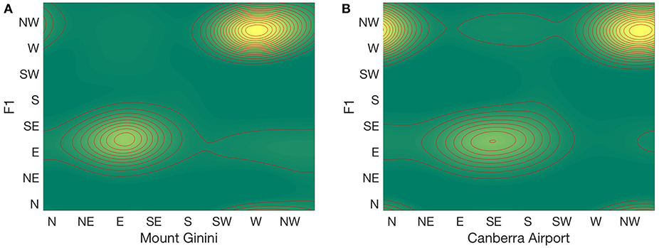
Figure 4. Joint wind direction distributions between F1 and (A) Mount Ginini and (B) Canberra Airport during the study period. Yellow coloring indicates higher frequency of wind direction pairs observed. Dotted line indicates equal wind direction at the two sites.

3. Methods

3.1. Conditional Wind Direction

The diagnostic wind model WindNinja was used to predict wind speed and wind direction across Flea Creek Valley using the SRTM 90 m digital elevation model, with the individual run calibrated to give a west-northwesterly wind direction at F1. Two solver options were used within the model; a mass conserving solver (packaged within WindNinja 2.5.2, referred to herein as the “native solver”), and a beta version of a mass and momentum conserving solver (later modified and released within WindNinja 3.0.0, referred to herein as the “momentum solver”). The model was run over a 10.3 km × 10.5 km domain with a vegetation choice of “Trees” and 1 ms⁻¹ domain-average wind speeds at 5 m above the vegetation layer. The selection of “Trees” allows a surface roughness length of 1 m with zero-plane displacement of 12 m (assuming a 15.4 m canopy height). The vegetation layer is also assumed to be uniform across the entire domain. Modeled wind directions were predicted to align with observations of WNW (298°) winds at F1 on the western ridge top. For each location, the modeled wind direction from a single model run was compared to the observed wind direction distributions, conditional on a WNW wind being observed at F1. Using a domain averaged wind speed of 1 ms⁻¹, modeled wind speeds at F1 were approximately 2 ms⁻¹ using both solvers.

As discussed previously, the wind field prediction was defined at 5 m above the vegetation layer, whereas wind observations were taken at 5 m above the ground within the approximately 15-m-high vegetation layer. To account for this in fire modeling applications, it is common to adjust wind speeds using wind reduction factors (e.g., Andrews, 2012; Quill et al., 2016; Moon et al., 2019), however wind directions are not transformed beneath the canopy. Therefore, the wind directions predicted at 5 m above the canopy using WindNinja are taken to indicate the predicted within-canopy wind directions used for operational fire modeling.

To compare the deterministically predicted wind direction to the observed conditional wind direction distribution, a percentage agreement value was calculated for the predicted wind direction segment. This was defined as the number of observations in the predicted segment as a proportion of the total observations for the time period.

3.2. Unconditional Wind Direction Distributions

For ensemble-based modeling of fire spread, input variables are varied around known distributions. For this purpose, it is therefore desirable to predict the probability distributions of wind speeds and directions. This study utilized a novel application of the deterministic WindNinja model to predict the distribution of wind direction at each location across Flea Creek Valley. Modeled unconditional wind direction distributions were constructed by running WindNinja with the momentum solver in an ensemble-type framework using the following procedure.

1. Generate look-up table: WindNinja was used to generate a wind direction look-up table for each site across the valley, using F1 as the reference station. Since the model is deterministic and the observations are discrete, it was only necessary to run WindNinja 16 times, each time calibrated to a different wind direction segment at F1. The look-up table therefore provided the modeled wind directions at each site, given the modeled wind direction at the reference station F1.

2. Model through time: Using the observed data at F1 as the representative domain average wind direction, the look-up table was cross-referenced to model wind direction at each site throughout the observation period. The look-up table, generated by the deterministic model, replaced the need to model the entire wind field at each time point.

3. Construct frequency distributions: The modeled time series were then used to construct modeled frequency distributions of wind direction at each site. The modeled wind direction distributions were compared to the unconditional distributions of all observed wind directions at each station site across the valley and throughout the study period.

To compare the modeled and observed unconditional wind direction distributions, both empirical and parametric measures are used. Firstly, the proportions of time that the predictions give a wind direction within the same wind direction sector, within one sector (±22.5°) and within two sectors (±45°) are calculated and analyzed. Secondly, the following 2-component mixture of von Mises distributions (often considered the circular equivalent to the Gaussian distribution) is fitted to the observed and predicted wind direction data (θ, in radians) for each site (Carta et al., 2008a);

$\begin{array}{rc}f(\theta ;p,{\mu }_1,{\kappa }_1,{\mu }_2,{\kappa }_2)=p\times g(\theta ;{\mu }_1,{\kappa }_1)+(1-p)\times g(\theta ;{\mu }_2,{\kappa }_2),& (1)\end{array}$

with

$\begin{array}{rc}g(\theta ;\mu ,\kappa )=\frac{1}{2\pi I_0(\kappa )}exp(\kappa cos(\theta -\mu )).& (2)\end{array}$

The function I₀(·) represents the modified Bessel function of the first kind and zeroth order, defined as

$\begin{array}{rc}{I}_0(\kappa )=\frac{1}{2\pi }{\displaystyle {\int }_0^{2\pi }}exp(\kappa cos\theta )d\theta .& (3)\end{array}$

The structures of the observed and predicted wind direction distributions are compared using the estimated parameters; p, the mixing proportions, μ_i, the mean direction of each component and κ_i, the concentration parameter of each component. Maximum likelihood estimation is used to fit the parameters of Equation (1) in MATLAB (2016).

4. Results

4.1. Deterministic Modeling of Conditional Wind Direction

Output from the single runs of both deterministic models (native solver and momentum solver) were analyzed in ArcGIS (ESRI, 2011) to generate the 5 meter predicted wind fields shown in Figures 5, 6. Table 3 shows the wind speed and wind direction outputs for each of the station sites. Using WindNinja with native solver (Figure 5), the predicted wind field was relatively smooth across the valley, maintaining a dominant WNW direction across both the leeward and windward slopes, as highlighted in the predictions given in Table 3. Wind speeds were highest across the western and eastern ridge tops, with very low speeds predicted on the valley floor.

FIGURE 5

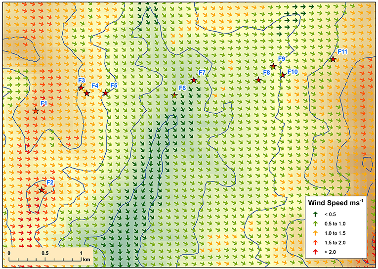
Figure 5. WindNinja with native solver prediction over Flea Creek Valley, using domain-average wind speeds of 1 ms⁻¹ and domain-average wind direction of 252°.

FIGURE 6

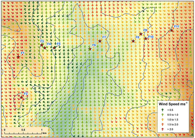
Figure 6. WindNinja with momentum solver prediction over Flea Creek Valley, using domain-average wind speeds of 1 ms⁻¹ and domain-average wind direction of 305°.

TABLE 3

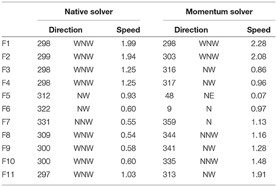
Table 3. Wind direction (°, compass point) and wind speed (ms⁻¹) predictions using WindNinja with native solver and momentum solver for each site across Flea Creek Valley.

Using the momentum solver (Figure 6), the domain-average wind direction was shifted significantly northward to achieve a WNW output at F1. This resulted in considerable northerly channeling through the valley. In addition, the predicted wind field using the momentum solver showed more spatial variation across the valley. This variation was most prominent on the leeward slope where, for instance, small lateral circulations were shown around gully features near F2 and F5. Wind speeds were again highest along the ridge tops, with the addition of some variations around small topographical features. In particular, wind speeds were shown to be much faster across the eastern windward slope around F10 and F12, as well as around F2 on the western ridge, than speeds modeled using the native solver.

Figure 7 shows the observed conditional wind direction distributions for a prevailing wind speed threshold of 0 ms⁻¹ and wind direction of WNW measured at F1. Predictions from Table 3 are shown in green for WindNinja with the native solver, and red for WindNinja with the momentum solver. Table 4 gives the proportion of the observed distributions that agree with each model prediction for increasing wind speed thresholds observed at F1. In general, the percentage agreements are low due to the deterministic nature of the individual predictions, with the individual model outputs not capable of capturing the variability of the observed wind direction distributions.

FIGURE 7

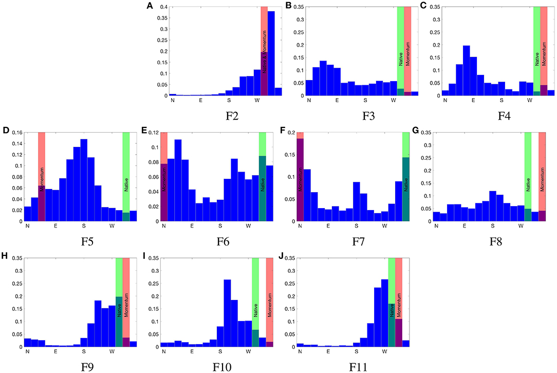
Figure 7. Observed wind direction distribution at sites (A–K) F1 to F11, across Flea Creek Valley, conditional on a WNW wind observed at F1. Predicted wind directions using WindNinja with native solver are indicated in green, and with momentum solver are indicated in red.

TABLE 4

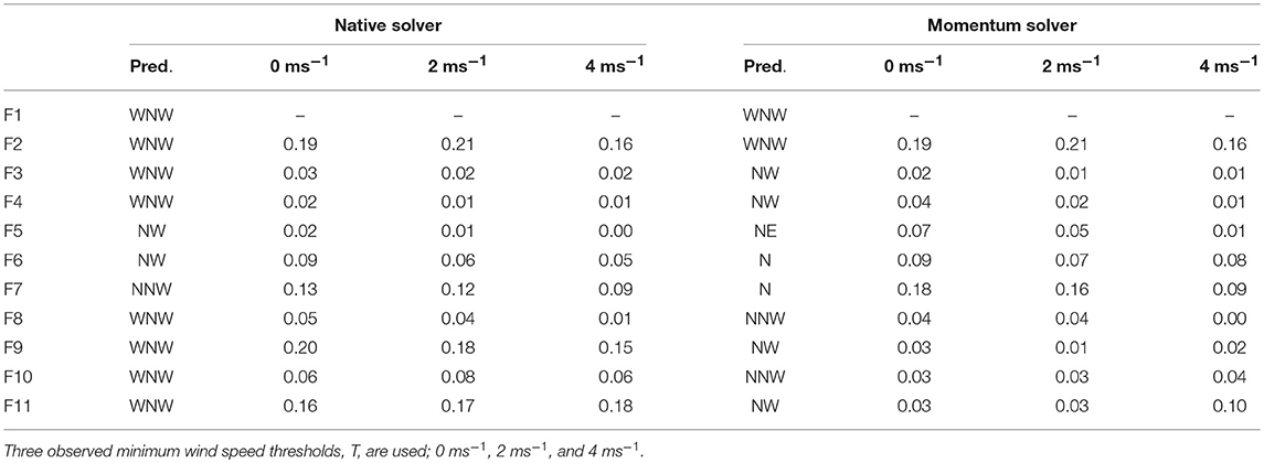
Table 4. Proportion of agreement between predicted wind direction (as compass point) and observed wind direction distribution at each site across Flea Creek Valley, conditional on observing a wind direction of WNW at F1.

The highest agreements for the deterministic predictions with either solver (Table 4), were found on the ridge tops (F2 and F11) and valley floor (F6 and F7) where the models predict the dominant wind direction modes of the broader scale wind field. On the western ridge top (F2), there is no difference between the predictions from either model, whereas on the eastern ridge top (F11) and valley floor (F6 and F7), the momentum solver prediction shows a bias toward northerly winds. This bias has little impact on the percentage agreements observed on the valley floor, but the agreement values between observation and prediction at F11 are much lower for the momentum solver than for the native solver at all wind speed thresholds, i.e., 2.5% at T = 0 ms⁻¹ as opposed to 15.6% for the native solver.

The highest individual deterministic agreement values were found at F2; with a wind speed threshold of 2 ms⁻¹, the percentage agreement reaches above 20% for both solvers. This agreement reduces at F2 as the wind speed threshold increases. Similar decreases in percentage agreement between model predictions and observations as wind speeds increase are shown across nearly all of the sites for both model versions.

On the western wall of the valley, leeward to the WNW prevailing winds, neither model predicts the easterly winds observed when applied as a single deterministic run. As seen in Figures 5, 6, the model with either solver predicts predominantly westerly flows across the entire valley when the prevailing winds are WNW. The observations at F3 and F4 clearly show dominant easterly modes at these stations (Figure 7), suggesting the existence of recirculation within the vegetation on the leeward slope. The discrepancies between predictions and observations result in extremely low agreement percentages of 3.2% or less for the native solver, and 3.7% or less for the momentum solver. This percentage agreements dropped to below 1% and 1.5% for the native and momentum solvers, respectively, as prevailing wind speeds increased.

Finally, on the eastern slope (F8, F9, and F10) single agreement percentages shown in Table 4 were larger than those shown for the western slope. The momentum solver predicts a considerable northerly bias to the flow through the valley, and this appears to have the greatest impact on the eastern slope. Therefore, the native solver performs better than the momentum solver at all three sites for all wind speed thresholds. In particular, at F9 the native solver predicts a WNW direction which captures the edge of the mode shown in Figure 7, while the momentum solver misses the mode by predicting a NW direction, resulting in agreement values of less than 3% as opposed to values up to 20% given by the native solver. This dramatic difference may in part be due to the discretization of wind direction, i.e., the binning of observations, which results in a significant difference in observations between two adjacent bins.

4.2. Modeling Unconditional Wind Direction Distributions

Figure 8 shows the observed unconditional wind direction distributions for each site across Flea Creek Valley (with a wind speed threshold of 0 ms⁻¹), as well as the predicted wind direction distributions produced using the probabilistic application of WindNinja with momentum solver. Table 5 shows the proportion of time that WindNinja, with the momentum solver, predicted the same wind direction as observed, or within one or two compass sectors (i.e., ±22.5° or ±45°). On the western and eastern ridge tops (F1 and F11, respectively), the predictions captured the dominant modal structures observed at the stations. In particular, at F1 the model captured the dominant WNW prevailing wind directions and the secondary easterly prevailing wind direction. At F11, although a bimodal distribution was predicted, the modes were concentrated, covering only a single wind direction bin.

FIGURE 8

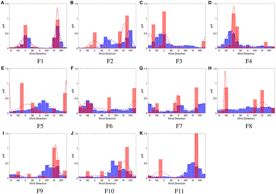
Figure 8. Observed (blue) and predicted (red, using momentum solver) unconditional wind direction distributions at sites (A–K) F1 to F11, across Flea Creek Valley. Dotted lines indicate fitted 2-component mixture von Mises distributions with parameters given in Table 6.

TABLE 5

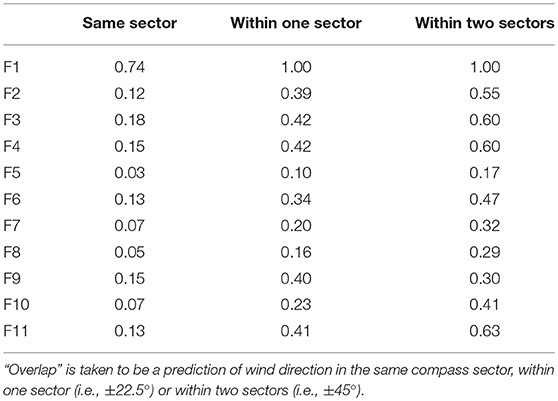
Table 5. Proportional overlap between predictions and observations at 1-min time steps.

For each site, the model generally predicts at least one mode coincident with the observed dominant wind direction shown in Figure 8. At F3 and F4, in contrast to the deterministic predictions, the predicted distributions pick up the wind reversal modes, i.e., the dominant easterly modes, with a relatively high prediction overlap of 60% within ±45° (Table 5). Similarly, at F9 and F10, the dominant westerly modes are better predicted than by the deterministic model. Through the valley floor (F6 and F7), the model indicates strong bimodal structures to the wind direction distributions which are somewhat evident in the observations but obscured by considerable variation.

Table 5 clearly shows the model to be accurate at the western ridge top (F1), with consistent wind direction predictions within one sector of the observations. At the remaining ridge top stations (F2 and F11), as well as on the western slope (F3 and F4) and on the eastern slope (F9), the model predicted wind directions within the same compass quadrant as those observed (i.e., within ±45°) over 50% of the time. As seen in the predicted distributions in Figure 8, these sites show the greatest similarity between the observed and predicted wind direction distributions.

The proportions of overlap between observed and predicted wind directions shown in Table 5 are lowest at locations across the valley where greater variation was observed (F5, F6, F7, F8, and F10). Table 5 shows an overlap within ±45° of 47% for F6, where a strong bimodal distribution was predicted, while a secondary wind direction mode was not strongly observed. The lowest overlap proportions are shown at F5, with only 17% overlap within two compass sectors. From the distribution shown in Figure 8, it is clear that the model did not capture the structure of the observed wind direction distribution.

Table 6 shows the maximum likelihood estimates for parameters of the 2-component mixture von Mises model used to fit the observed and predicted wind direction distributions. In general, the predicted distributions show modes with considerably higher concentration parameters, showing the models inability to capture the observed variability in wind direction. However, many location parameters were well predicted, with mismatched location estimates potentially due to small-scale topography or high variability which were unable to be resolved by the deterministic model, i.e., F2, F5, and F8.

TABLE 6

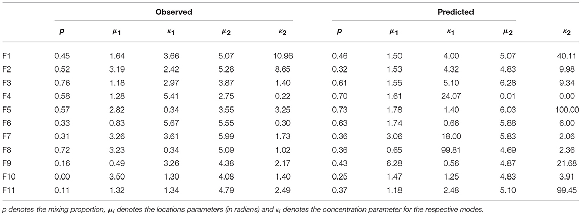
Table 6. Estimated parameters for a 2-component mixture von Mises model fit to the observed and predicted wind direction distributions across Flea Creek Valley.

For stations with clearly observed and predicted bimodal distributions, the 2-component mixture von Mises parameter estimates give similar location parameters, i.e., F1, F7, F9, F10, and F11. However, for other distributions (both observed and predicted) the 2-component mixture may not be the most appropriate fit. For example, F3 and F4 appear to show unimodal distributions, and so the estimated bimodal parameters either show an extremely unbalanced mix (i.e., predicted mixture at F4 gives κ₁ = 24.07 and κ₂ = 0.00), or modes at close locations (i.e., predicted mixture at F3 gives μ₁ = 1.55 and μ₂ = 6.28). For stations with very high observed variability such as F8, the predicted and observed parameter estimates were very poorly aligned; firstly, the location parameter for the observed distribution had limited meaning with such low concentration parameters, and secondly the predicted distribution had far greater concentrations than observed.

5. Discussion

5.1. Deterministic Modeling

In general, the best agreement between the individual deterministic predictions and the conditional wind direction distributions occurred on the ridges and valley floor. These areas can be thought to represent broader scale terrain features, while the valley sides represent areas where more complex physical features dominate wind flows, such as the recirculation regions on leeward slopes caused by flow separation over ridges. As discussed in the introduction, the modeling framework behind the WindNinja software simplifies some of the physical equations governing such flows to enable operational use, and thus is known to be limited in such areas (Forthofer et al., 2014b). The results of the deterministic application in this study further confirm this, but add probabilistic information to these limitations, finding that percentage agreements at individual sites can be extremely low.

With the addition of the momentum solver, WindNinja was able to better capture some topographic impacts on wind flow across the valley, including recirculation within gullies and on leeward slopes, and larger-scale channeling along the valley floor. With a comparison of only a select few individual sites, the ability of the momentum solver to capture some of these more complex flows is not shown with the analysis presented here. For example, on the leeward slope, recirculation is not predicted within the pixel overlapping the two observation sites, yet it is observed elsewhere on this slope in Figure 2. The discrete nature of the observed wind direction (22.5° sectors) may also contribute to some of the low percentage agreement values seen throughout this analysis. Through estimation of distributions in the ensemble-style analysis, some of these discrepancies may be smoothed.

Other broad-scale flows shown by the deterministic momentum solver prediction, such as the strong northerly bias on the eastern slopes, was not observed in the data. This northerly-skewed prediction by the momentum solver was due to the adaptation of input parameters to optimize the model run but led to lower performance on the windward slope—reducing percentage agreements from 20% with the native solver down to only 3%. In the context of fire, this significant difference between predicted and observed wind direction may cause considerable difference between predicted and observed fire spread.

Across the valley, it is shown that as observed wind speed thresholds increase, the percentage agreement between the individual predictions and observed conditional wind direction distributions decreases. This decrease is to be expected since analysis [not shown here, but also highlighted by Sharples et al. (2010)] indicates that the variance of dominant modes decreases as wind speed thresholds increase, resulting in a lower percentage agreement if the model does not accurately predict the key mode. Due to the relatively low wind speeds experienced throughout the study period the highest wind speed thresholds also have smaller sample sizes to construct the distributions for comparison, thus somewhat reducing the reliability of subsequent conclusions. Further model runs with higher domain-averaged wind speed, larger simulation domains and higher model resolution might also indicate different predicted behaviors across the region. However, it was found that increased wind speeds under the native solver had little impact on predicted wind direction.

The lack of a diurnal pattern at F3 and F4, as shown in Figure 3, and the persistence of lee-slope easterly modes under higher wind speed conditions suggests that they are due to recirculation eddies driven by flow separation over the leeward slope rather than upslope thermal winds. Analysis of the timing of similar easterly modes experienced in the same location across the valley by Sharples et al. (2010) also showed limited diurnal patterns, suggesting that this recirculation region is in fact an area of persistent lee-slope eddies within the vegetation layer. Another possibility is that the easterly modes could be due to pressure-driven recirculation under the canopy but given the agreement between these results and those of Sharples et al. (2010), which were obtained in the absence of an intact canopy, flow separation is likely the main driver. While WindNinja with either solver is not intended to predict within canopy flows, with no mechanism for wind direction adjustment, these eddies are consequently often not captured within fire modeling frameworks.

5.2. Modeling Wind Direction Distributions

The ensemble-style application of WindNinja, using wind libraries, allows for a prediction of the full distribution of wind direction at each point across the valley. This probabilistic representation of wind predictions is better suited to emerging ensemble-style fire modeling frameworks, where uncertainty can be quantified and analyzed. In general, the ensemble-style application of WindNinja with momentum solver predicted coincidental modes for wind direction distributions across the valley. However, the modeled data shows considerably lower variation than the observed.

The limited predicted variation is to be expected due to the deterministic nature of the model, with simplified physical equations. Equally, the model predicts above canopy winds while observations were taken beneath the canopy, thus influenced by additional turbulence. Despite this, the within canopy winds showed distinct structures which evidence the existence of consistent wind behaviors such as beneath canopy recirculation zones. Due to the lack in predicted variability, the model was least effective at the most variable sites, where wind speeds were low. In areas where wind directions were highly variable, overlap percentages (to within an entire compass quadrant) could be as low as 17%, and estimated location and concentration parameters were poorly aligned. However, it should be noted, that at some sites, the estimation of a 2-component mixture distribution may be inappropriate, leading to misalignment between observation and prediction estimates. A more flexible modeling approach may be required, where the number of mixture components is also a parameter to be estimated.

The high variation in the wind directions observed at the valley floor sites, reduces the efficacy of the prediction, but the variation itself may also be induced by local features affecting the wind field which are not adequately resolved by the model. For instance, F6 is located on top of a knoll at the bottom of the valley which may induce localized flows or eddies which cannot be represented at the resolution used to predict the wind field. This is again evident at F8 on the eastern slope; observed wind directions are almost uniform around the compass, whereas the model predicts an approximately bimodal distribution representative of mechanical valley winds.

Indeed, there are clearly other factors that influence the variability of wind directions (and wind speeds), aside from the prevailing wind direction. It is this heterogeneity in variation across the landscape (particularly in relation to deterministic predictions) that requires further study to understand how to best account for these factors in deterministic models (yet maintain computational efficiency). Probabilistic approaches may help to fill such gaps with efficient statistical wind models that can inherently capture heterogeneity in relationships between influencing factors across spatial domains.

6. Conclusion

In the pursuit of accurate fire spread prediction, the accuracy of model inputs must be considered. In emerging bushfire research, the accuracy of outputs is being framed in terms of uncertainty, with an increasing focus on ensemble methods and probabilistic representations. Traditional deterministic models must now be complemented with probabilistic information informed by empirical data. This study shows a stark comparison between the application of a diagnostic wind model using the traditional approach and a novel ensemble-style application. The demonstrated ability of this novel method in capturing observed wind field variability highlights a significant advance in modeling input variables (not limited to wind fields) and forms an understanding of the uncertainty in ensemble-based bushfire prediction.

The application of WindNinja with both native and momentum solvers is limited by its deterministic nature, leading to small agreement percentages between single predictions and observed wind direction distributions. As previously noted in the literature (Forthofer et al., 2014a,b; Butler et al., 2015; Wagenbrenner et al., 2016), the models perform poorly on the leeward slopes, with observations representative of recirculation regions not captured at the study sites. However, some areas of recirculation were predicted by the momentum solver in other areas of the leeward slope. It has been shown in the literature that lee-slope eddies can create necessary conditions for dangerous and extreme fire behavior (Sharples et al., 2012; Simpson et al., 2013), and the inability of a single model run to identify such wind behaviors can lead to the misrepresentation of fire spread and behavior across the landscape. Individual model runs can be extremely sensitive to the set of input variables, including domain-averaged wind direction as well as the size and resolution of the domain. Fire managers are encouraged to better understand this sensitivity by running multiple wind input scenarios, however, very limited formal sensitivity analysis exists within the literature. Quantifying the effects of probabilistic prediction of input variables, including wind speed and direction, is an ongoing focus of further research in wildland fire prediction.

The novel ensemble-style application of WindNinja with the momentum solver resulted in the modeling of wind direction distributions which were able to capture some of the key structures of wind flow observed across the valley. Bimodal distributions were predicted at a number of sites where the deterministic application of the model was only able to predict a single outcome. In particular, predicted distributions were able to capture observed leeward slope recirculation which would lead to a strengthened ability of fire models to identify regions prone to extreme and erratic fire behavior. Although distributional predictions were able to model key wind direction modes at each site, the predictions lacked considerable variability compared to observed distributions.

There is always room for improvement to better capture underlying physical processes, but dynamic downscaling models can still be limited by resolution. Mechanisms existing at finer scales will continue to contribute uncertainty to model outputs. From this study, it is clear that an ensemble-style application of WindNinja shows differing levels of accuracy across the landscape, where different physical processes may dominate wind flow. To address some of these gaps, physical processes can be modeled using probabilistic approaches. While statistical approaches have their own limitations, such as relying upon previous system behaviors (including outliers), they are able to capture some of the variability of wind and fire spread across the landscape, which is not resolved by current physical models and can be better suited to emerging ensemble-based fire prediction frameworks. Probabilistic models not only provide more informative inputs for bushfire prediction but can also be used to identify areas where different driving forces may have varying impacts on fire behavior, such as significant terrain effects or fire-atmosphere coupling. In additional further research, sensitivity analysis of fire modeling frameworks is required to understand the quantitative effects of capturing (or not capturing) the true variability of wind fields over complex terrain. Using such analysis alongside ensemble-based or probabilistic modeling approaches will allow for formal and quantitative assessments of uncertainty in operational fire spread and behavior predictions.

Data Availability

The dataset analyzed for this study can be found in the University of Adelaide Figshare repository: Flea Creek Valley Data, Jul to Dec 2014 (Quill and Sharples, 2018), accessed via https://doi.org/10.25909/5c13258d1407a.

Author Contributions

RQ, JS, and LS conceived and designed the initial study, with further development provided by NW and JF. RQ coordinated the study. RQ and JS undertook data collection. RQ and NW conducted the analysis and modeling, with JS, LS, and JF providing critical comments. RQ drafted the manuscript. JS, NW, LS, and JF provided revisions of the manuscript. All authors read and approved the final manuscript.

Funding

RQ acknowledges the financial support of UNSW Canberra and the Bushfire and Natural Hazards Cooperative Research Centre (BNHCRC; Ref: RG142924) in conducting this research.

Conflict of Interest Statement

The authors declare that the research was conducted in the absence of any commercial or financial relationships that could be construed as a potential conflict of interest.

Footnotes

1. ^https://www.firelab.org/project/windninja

References

Albini, F. A. (1976). Estimating Wildfire Behavior and Effects. General Technical Report Int-30. Report, USDA Forest Service, Intermountain Forest and Range Experiment Station, Ogden, UT.

Alegría, A., Bevilacqua, M., and Porcu, E. (2016). Likelihood-based inference for multivariate space-time wrapped-Gaussian fields. J. Stat. Comput. Simulat. 86, 2583–2597. doi: 10.1080/00949655.2016.1162309

CrossRef Full Text | Google Scholar

Alexander, M. E., and Cruz, M. G. (2013). Limitations on the accuracy of model predictions of wildland fire behaviour: a state-of-the-knowledge overview. For. Chronic. 89, 372–383. doi: 10.5558/tfc2013-067

CrossRef Full Text | Google Scholar

Andrews, P. L. (2012). Modeling Wind Adjustment Factor and Midflame Wind Speed for Rothermel's Surface Fire Spread Model. United States Department of Agriculture/Forest Service, Rocky Mountain Research Station. doi: 10.2737/RMRS-GTR-266

CrossRef Full Text

Belcher, S. E., Harman, I. N., and Finnigan, J. J. (2012). The wind in the willows: flows in forest canopies in complex terrain. Annu. Rev. Fluid Mech. 44, 479–504. doi: 10.1146/annurev-fluid-120710-101036

CrossRef Full Text | Google Scholar

Butler, B. W., Wagenbrenner, N. S., Forthofer, J. M., Lamb, B. K., Shannon, K. S., Finn, D., et al. (2015). High-resolution observations of the near-surface wind fields over an isolated mountain and in a steep river canyon. Atmospher. Chem. Phys. 15, 3785–3801. doi: 10.5194/acp-15-3785-2015

CrossRef Full Text | Google Scholar

Carta, J. A., Bueno, C., and Ramírez, P. (2008a). Statistical modelling of directional wind speeds using mixtures of von Mises distributions: case study. Energy Convers. Manage. 49, 897–907. doi: 10.1016/j.enconman.2007.10.017

CrossRef Full Text | Google Scholar

Carta, J. A., Ramírez, P., and Bueno, C. (2008b). A joint probability density function of wind speed and direction for wind energy analysis. Energy Convers. Manage. 49, 1309–1320. doi: 10.1016/j.enconman.2008.01.010

CrossRef Full Text | Google Scholar

Cruz, M. G. (2010). Monte carlo-based ensemble method for prediction of grassland fire spread. Int. J. Wildl. Fire 19, 521–530. doi: 10.1071/WF08195

CrossRef Full Text | Google Scholar

Cruz, M. G., and Alexander, M. E. (2013). Uncertainty associated with model predictions of surface and crown fire rates of spread. Environ. Modell. Softw. 47, 16–28. doi: 10.1016/j.envsoft.2013.04.004

CrossRef Full Text | Google Scholar

Erdem, E., and Shi, J. (2011). Comparison of bivariate distribution construction approaches for analysing wind speed and direction data. Wind Energy 14, 27–41. doi: 10.1002/we.400

CrossRef Full Text | Google Scholar

ESRI (2011). ArcGIS Desktop: Release 10. Redlands, CA: Environmental Systems Research Institute.

Finney, M. A., Grenfell, I. C., McHugh, C. W., Seli, R. C., Trethewey, D., Stratton, R. D., et al. (2011). A method for ensemble wildland fire simulation. Environ. Model. Assess. 16, 153–167. doi: 10.1007/s10666-010-9241-3

CrossRef Full Text | Google Scholar

Finnigan, J. (2000). Turbulence in plant canopies. Annu. Rev. Fluid Mech. 32, 519–571. doi: 10.1146/annurev.fluid.32.1.519

CrossRef Full Text | Google Scholar

Finnigan, J. J., and Belcher, S. E. (2006). Flow over a hill covered with a plant canopy. Q. J. R. Meteorol. Soc. 130, 1–29. doi: 10.1256/qj.02.177

CrossRef Full Text | Google Scholar

Forthofer, J. M. (2007). Modelling Wind in Complex Terrain for Use in Fire Spread Prediction. Thesis, Department of Forest, Rangeland and Watershed Stewardship, Colorado State University.

Forthofer, J. M., Butler, B. W., McHugh, C. W., Finney, M. A., Bradshaw, L. S., Stratton, R. D., et al. (2014a). A comparison of three approaches for simulating fine-scale surface winds in support of wildland fire management. Part II. an exploratory study of the effect of simulated winds on fire growth simulations. Int. J. Wildl. Fire 23, 982–994. doi: 10.1071/WF12090

CrossRef Full Text | Google Scholar

Forthofer, J. M., Butler, B. W., and Wagenbrenner, N. S. (2014b). A comparison of three approaches for simulating fine-scale surface winds in support of wildland fire management. Part I. Model formulation and comparison against measurements. Int. J. Wildl. Fire 23, 969–981. doi: 10.1071/WF12089

CrossRef Full Text | Google Scholar

French, I., Cechet, B., Yang, T., and Sanabria, A. (2013). “FireDST: fire impact and risk evaluation decision support tool-model description,” in MODSIM2013, 20th International Congress on Modelling and Simulation, eds J. Piantadosi, R. S. Anderssen, and J. Boland (Adelaide, SA: Modelling and Simulation Society of Australia and New Zealand Inc.).

Google Scholar

French, I. A., Duff, T. J., Cechet, R. P., Tolhurst, K. G., Kepert, J. D., and Meyer, M. (2014). “FireDST: a simulation system for short-term ensemble modelling of bushfire spread and exposure,” in Advances in Forest Fire Research, ed D. X. Viegas (Coimbra: Imprensa da Universidade de Coimbra), 1147–1158.

Google Scholar

Kourtz, P. (1972). Probability makes fire danger index more reliable. Fire Control Notes 33, 11–12.

Google Scholar

Lagona, F., and Picone, M. (2016). Model-based segmentation of spatial cylindrical data. J. Stat. Comput. Simulat. 86, 2598–2610. doi: 10.1080/00949655.2015.1122791

CrossRef Full Text | Google Scholar

Lopes, A. M. G. (2003). WindStation: a software for the simulation of atmospheric flows over complex topography. Environ. Model. Softw. 18, 81–96. doi: 10.1016/S1364-8152(02)00024-5

CrossRef Full Text | Google Scholar

MATLAB (2016). R2016b. Natick, MA: The MathWorks, Inc.

McRae, R. H. D. (2004). “Breath of the dragon–observations of the January 2003 ACT bushfires,” in Proceedings of Bushfire 2004 (Adelaide, SA).

Google Scholar

McRae, R. H. D., and Sharples, J. J. (2013). “A process model for forecasting conditions conducive to blow-up fire events,” in MODSIM2013, 20th International Congress on Modelling and Simulations, eds J. Piantadosi, R. S. Anderssen, and J. Boland (Adelaide, SA: Modelling and Simulation Society of Australia and New Zealand), 2506–2512.

Google Scholar

Moon, K., Duff, T. J., and Tolhurst, K. G. (2019). Sub-canopy forest winds: understanding wind profiles for fire behaviour simulation. Fire Saf. J. doi: 10.1016/j.firesaf.2016.02.005. [Epubh ahead of print].

CrossRef Full Text | Google Scholar

Noble, I. R., Gill, A. M., and Bary, G. A. V. (1980). McArthur's fire-danger meters expressed as equations. Aust. J. Ecol. 5, 201–203. doi: 10.1111/j.1442-9993.1980.tb01243.x

CrossRef Full Text | Google Scholar

Penman, T. D., Collins, L., Price, O. F., Bradstock, R. A., Metcalf, S., and Chong, D. M. O. (2013). Examining the relative effects of fire weather, suppression and fuel treatment on fire behaviour - a simulation study. J. Environ. Manage. 131, 325–333. doi: 10.1016/j.jenvman.2013.10.007

PubMed Abstract | CrossRef Full Text | Google Scholar

Quill, R. (2017). Statistical Characterisation of Wind Fields Over Complex Terrain With Applications in Bushfire Modelling. Thesis, School of Physical, Environmental and Mathematical Sciences, UNSW Canberra.

Quill, R., Moon, K., Sharples, J. J., Sidhu, L. A., Duff, T. J., and Tolhurst, K. G. (2016). “Wind speed reduction induced by post-fire vegetation regrowth,” in Research Forum at the Bushfire and Natural Hazards CRC & AFAC Conference, ed M. Rumsewicz (Brisbane, QLD: Bushfire and Natural Hazards CRC), 15–29.

Quill, R., and Sharples, J. J. (2018). Flea Creek Valley Data, Jul to Dec 2014. Figshare. doi: 10.25909/5c13258d1407a

CrossRef Full Text

Sharples, J. J., McRae, R. H. D., and Weber, R. O. (2010). Wind characteristics over complex terrain with implications for bushfire risk management. Environ. Model. Softw. 25, 1099–1120. doi: 10.1016/j.envsoft.2010.03.016

CrossRef Full Text | Google Scholar

Sharples, J. J., McRae, R. H. D., and Wilkes, S. R. (2012). Wind–terrain effects on the propagation of wildfires in rugged terrain: fire channelling. Int. J. Wildl. Fire 21, 282–296. doi: 10.1071/WF10055

CrossRef Full Text | Google Scholar

Simpson, C. C., Sharples, J. J., Evans, J. P., and McCabe, M. F. (2013). Large eddy simulation of atypical wildland fire spread on leeward slopes. Int. J. Wildl. Fire 22, 599–614. doi: 10.1071/WF12072

CrossRef Full Text | Google Scholar

Tolhurst, K. G., Shields, B., and Chong, D. (2008). Phoenix: development and applications of a bushfire risk management tool. Austral. J. Emerg. Manage. 23, 47–54.

Google Scholar

Twomey, B., and Sturgess, A. (2016). “Simulation analysis-based risk evaluation (SABRE) fire: operational stochastic fire spread decision support capability in the Queensland Fire and Emergency Service,” in Proceedings of AFAC 2016 (Brisbane, QLD).

Google Scholar

Wagenbrenner, N. S., Forthofer, J. M., Lamb, B. K., Shannon, K. S., and Butler, B. W. (2016). Downscaling surface wind predictions from numerical weather prediction models in complex terrain with WindNinja. Atmos. Chem. Phys. Discuss. 2016, 1–32. doi: 10.5194/acp-2015-761

CrossRef Full Text | Google Scholar