A Methodology for Studying the Relationship Between Heat Release Profile and Fuel Stratification in Advanced Compression Ignition Engines

Introduction

In response to stricter regulations of pollutant emissions placed on light-duty and heavy-duty vehicles by governmental agencies (U.S. EPA and DOT, 2012; U.S. EPA, 2016) due to concerns over local air pollution and the depletion of fuel stocks over the past 40 years, researchers have sought new, and novel combustion strategies. These strategies avoid the typical pollutant emissions issues associated with conventional diesel and spark ignited engine platforms, while simultaneously providing methods to increase fuel economy. Compression ignition strategies, in particular, have garnered significant interest due to their potential for high thermodynamic efficiency, and low fuel consumption. Combustion strategies which are able to avoid locally rich and high temperature regions can simultaneously avoid the formation of soot and NO (Neely et al., 2005); however those combustion strategies that avoid high temperature regions often result in high carbon monoxide and unburned hydrocarbon emissions (Kim et al., 2008). One such group of strategies, collectively referred to as low temperature combustion (LTC) modes, or advanced compression ignition (ACI) modes, includes strategies such as homogeneous charge compression ignition (HCCI), partially premixed combustion (PPC), partial fuel stratification (PFS), gasoline compression ignition (GCI), and reactivity controlled compression ignition (RCCI). While these strategies primarily differ in the amount of in-cylinder fuel stratification induced by the direct injection strategy, they all seek to take advantage of the low temperature, kinetically controlled combustion regime characterized by low pollutant emissions resulting from lean air-fuel mixtures (Neely et al., 2005), and high thermal efficiencies from reduced heat transfer losses and short combustion durations (Splitter et al., 2011; Northrop et al., 2013).

The earliest form of low temperature combustion studied was homogeneous charge compression ignition (HCCI), which utilizes a fully premixed charge of fuel and air at lean equivalence ratios (φ < 1.0), which is compressed until autoignition. The strategy relies on long ignition delays, which are achieved by operating with high levels of dilution either by increasing intake pressure, resulting in a decrease in equivalence ratio, or by adding exhaust gas recirculation (EGR). High levels of dilution reduce peak in-cylinder temperatures, thereby reducing NO_x formation, and operating at globally lean conditions typically results in lower PM formation and emissions. The earliest HCCI research performed on four stroke engines was performed by Najt and Foster (1983), who found that the response of the combustion process of HCCI to operating parameters could be explained by the fuel chemical kinetics. The kinetically controlled nature of the combustion strategy means that the combustion phasing is very sensitive to the in-cylinder temperature distribution, the intake pressure, global equivalence ratio, and the fuel properties. However, the early injection strategy provides no direct means of controlling the combustion process. Significant research on HCCI has focused on the role of thermal stratification in HCCI combustion (Dec and Sjöberg, 2004; Sjöberg et al., 2004, 2005; Sjöberg and Dec, 2005; Dec et al., 2006; Dec and Hwang, 2009; Snyder et al., 2011; Lawler et al., 2012, 2014a,b), and the results have shown that ignition tends to propagate following the thermal gradients in the cylinder, starting in the highest temperature regions (Fiveland and Assanis, 2001). However, the HCCI strategy tends to suffer from high cycle-to-cycle variability due to its sensitivity to variations in the charge composition and in-cylinder thermal stratification, and while thermodynamically attractive, HCCI combustion is limited to a narrow operable load range that is a function of the particular fuel properties. Excessive pressure rise rates can occur at high load, which can result in engine damage, and high CO and UHC emissions and poor combustion stability is seen at low load (Bessonette et al., 2007).

To combat the inherent weakness of the HCCI strategy (namely the lack of direct combustion control), strategies utilizing direct injection of a fraction of the total fuel were developed to provide in-cylinder equivalence ratio stratification. These strategies include partially premixed combustion (PPC), and partial fuel stratification (PFS). The two strategies differ primarily by the fraction of the total fueling that is stratified (~10–20% for PFS and ~25–50% for PPC). The equivalence ratio stratification induced by the direct injection event has been shown by researchers to provide significantly improved control over the heat release event compared to fully-premixed HCCI combustion (Dec and Sjöberg, 2004; Sjöberg and Dec, 2006, 2011; Hwang et al., 2007; Dec et al., 2011; Yang et al., 2011, 2012). This fuel stratification allows for the extension of the load range relative to a single fuel fully-premixed HCCI strategy at low loads (Hwang et al., 2007; Manente et al., 2010a; Bakker et al., 2014), and high loads (Manente et al., 2010a,b; Lewander et al., 2011; Dec et al., 2012), though high peak pressure rise rates and limited direct control over combustion are still a challenge for PPC and PFS strategies.

Work by Bessonette et al. (2007) showed that the optimal fuel for HCCI combustion had an octane number between that of diesel and gasoline, and that the desired octane number was a function of engine load. Additionally, Inagaki et al. (2006) demonstrated that in-cylinder fuel blending of fuels with different properties could provide good combustion control with low emissions. Motivated by this, Kokjohn et al. (2009) outlined the RCCI strategy, which involved port injection of a low reactivity fuel (e.g., gasoline) and multiple direct injections of a high reactivity fuel (e.g., diesel) to provide coupled equivalence ratio and reactivity gradients in the cylinder. These reactivity gradients provide good control over the combustion phasing and heat release rate as the injection timing and ratio of premixed to direct injected fuel can be adjusted independently, providing a range of operable conditions for a given speed/load point. Subsequent work by many researchers have demonstrated a wide operable load range for RCCI combustion in both light and heavy-duty engine platforms with low NOx and PM emissions utilizing a variety of high and low reactivity fuel sources (Curran et al., 2010, 2012, 2013, 2014; Hanson et al., 2010, 2011, 2013; Splitter et al., 2010, 2011, 2012, 2013, 2014; Splitter and Reitz, 2014) RCCI combustion has also demonstrated significant control over combustion phasing and heat release rate with moderate peak pressure rise rates relative to HCCI combustion (Splitter, 2012; Splitter et al., 2012, 2014). This controllability is a direct result of the equivalence ratio and reactivity stratification induced by direct injection of the high reactivity fuel.

Optical engine work by Kokjohn et al. (2012) demonstrated the effects of fuel distribution due to injection timing in RCCI combustion with iso-octane as the premixed fuel and n-heptane as the direct injected fuel, and showed the large degree of control over the shape and phasing of the combustion event that the RCCI strategy yields, while Splitter (2012) showed the effect of mixture stratification due to injection timing and number of injections on performance and losses in RCCI combustion. The increase in thermal efficiency of the RCCI strategies compared to HCCI was attributed to the decrease in heat transfer and exhaust losses due to the decreased pressure rise rate induced by the reactivity and equivalence ratio gradients in the cylinder, despite the associated increase in combustion losses (Splitter, 2012). Similar to Kokjohn et al. (2012), Splitter (2012) showed that the optimal dual fuel strategy occurred somewhere between the fully premixed cases and overly stratified late injection timings.

The inspiration for the present work stems from an analysis methodology called Thermal Stratification Analysis (TSA) proposed by Lawler et al. (2012), which used the autoignition integral described in Livengood and Wu (1954), in combination with experimentally derived mass fraction burned curves, in order to determine the distribution of temperature in the combustion chamber due to natural thermal stratification in HCCI engines. The analysis breaks the cylinder into many thermal zones, each following a different self-similar temperature profile during the compression and expansion process, and correlates the ignition locations of these various zones to mass fraction burned data to derive cumulative density functions (CDFs), and probability density functions (PDFs) of the in-cylinder temperature distribution (Lawler et al., 2012). Further improvements in the TSA methodology, particularly for handling the low temperature end of the distribution, as well as validation with CFD and optical engine data were published by Lawler et al. (2014a). In general, the TSA predictions did a good job predicting the thermal stratification present in HCCI combustion. Unfortunately, due to the nature of HCCI combustion, these results do not have a great amount of practical significance as thermal stratification cannot be easily controlled, except by adjusting the coolant temperature (which is a parameter adjusted in the steady state experiments by Lawler et al. (2012, 2014a) or oil temperature, which have significant time lags associated with them, making next cycle control of HCCI combustion with these parameters impossible. As discussed previously, the biggest challenge facing HCCI combustion is the significant cycle-to-cycle variability associated with the strategy, as well as the lack of a direct combustion rate control mechanism. While thermal stratification is the main parameter for heat release rate control in HCCI combustion, this factor is not as easily manipulated as the stratification of fuel induced by direct injection events, which has been shown to produce significantly improved heat release rate control and combustion stability (Sjöberg and Dec, 2006, 2011; Hwang et al., 2007; Dec et al., 2011; Yang et al., 2011, 2012). A methodology similar to the TSA approach, but applied to fuel stratification instead of thermal stratification would provide much more valuable information regarding the fuel distributions present in kinetically controlled combustion strategies such as PPC, PFS, GCI, and RCCI, as well as help to specify fuel stratification requirements for these strategies for conventional and alternative fuels.

The authors' experimental data presented in DelVescovo et al. (2017), and previous work comparing the performance and emissions characteristics of gasoline/diesel RCCI operation to RCCI experiments using isobutanol as the low and high reactivity fuel (DelVescovo et al., 2015), has shown the importance of tailoring the direct injection strategy to the specific fuel combination to maximize performance and minimize emissions. Comparing cases using methane and syngas as the low reactivity fuel to baseline iso-octane/n-heptane cases showed the importance of matching the bulk heat release characteristics, including phasing, duration, and rates, and if this could be achieved, the performance and emissions could attain rates comparable to the baseline condition (DelVescovo et al., 2017). In stratified kinetically controlled combustion strategies such as RCCI, the heat release shape is defined by the gradients of in-cylinder reactivity and equivalence ratio, which are directly related to the direct injection strategy through injection timing, injection pressure, and number of injections. Assuming some arbitrary optimal heat release profile, it would be beneficial to determine the required distribution of fuel necessary to achieve such a heat release a priori, without extensive, and costly experimental or modeling effort. This notion serves as the motivation for the model referred to as Fuel Stratification Analysis (FSA) proposed in this work. This manuscript is arranged as follows: first, the methodology is described in detail, including all relevant assumptions and analysis, next reacting 3-D CFD simulations are validated against experimental HCCI and RCCI data, and finally, the FSA methodology is validated against non-reacting 3-D CFD simulations to assess the validity and predictive capability of the methodology, followed by a discussion of the potential applications of the FSA approach.

Methodology

The major difference between the TSA and FSA methodologies is that the mixture composition is not assumed to be uniform throughout the combustion chamber. The combustion process in single-fuel stratified-charge strategies such as PFS, as well as dual-fuel stratified-charge strategies such as RCCI, has been shown to propagate by sequential autoignition from the most reactive regions to the least reactive regions (Dec et al., 2006; Kokjohn et al., 2009, 2015; Sjöberg and Dec, 2011; Kokjohn, 2012; Wolk et al., 2015), where reactivity is effectively a measure of the relative ignition delay of the fuel/oxidizer mixture at its thermodynamic state. Dec et al. (2006) showed that even with a perfectly homogeneous fuel distribution, thermal stratification in HCCI combustion resulted in sequential autoignition from hotter-to-cooler regions, implying that high temperature regions are more reactive than low temperature regions. This sequential autoignition from hot-to-cold mixtures is the basis for the TSA method, and sequential autoignition from high reactivity (induced by fuel chemistry and/or high equivalence ratio) to low reactivity is the basis for the present proposed FSA method.

Initializing Zones

Similar to the TSA method, which utilizes a normalized zone temperature to define the various possible thermal pathways in the cylinder (Lawler et al., 2012), a non-dimensional, normalized parameter is defined to establish the possible fuel mixtures that may exist within the cylinder. This parameter, referred to as the premixed mass fraction (PRE), expresses the ratio of premixed fuel mass in a given “zone” or “region” to the total fuel mass in the zone, i.e., PRE = 1 means that the zone only contains premixed (low reactivity) fuel, PRE = 0 means that a zone contains only direct-injected fuel, which, despite being impossible assuming that the premixed fuel is thoroughly mixed, defines the lower bound of possible fuel mixtures. The premixed percentage, which is the premixed fraction multiplied by 100, is approximately equal to the local PRF number if the premixed fuel is isooctane and the direct injected fuel is n-heptane. In these situations, the premixed percent and PRF number will be used interchangeably. This ignores the small difference in density between the two fuels, as PRF number is defined on a volumetric instead of mass basis. The maximum error of this assumption occurs at PRF50, and is equal to only 0.29% (i.e., PRF50 is 50.29% by mass isooctane). Equation (1) shows the relationship for the premixed mass fraction, and the direct injected mass in the zone (m_DI,i) can be determined by assuming some arbitrary value of PRE_i, where the “i” subscript indicates the i^th zone. This relationship is shown in Equation (2).

$\begin{array}{ll}PR{E}_i=\frac{m_{premixed}}{m_{premixed}+m_{DI,i}}& (1)\end{array}$

$\begin{array}{ll}{m}_{DI,i}=m_{premixed}\left(\frac{1}{PR{E}_i}-1\right)& (2)\end{array}$

The premixed mass (m_premixed) in the above equations does not necessarily correspond to the actual mass of premixed fuel in a zone, as the relative distribution of mass is yet unknown. For the purposes of this analysis, m_premixed is the premixed fuel fraction, i.e., the analysis is performed on the basis of one unit of global fuel mass. This relative mass is used only to define the mixture properties of the zone, such as the equivalence ratio, ϕ_i, the relationship for which can be seen in Equation (3). The zone air-fuel ratio (AFR_i) can then be calculated by dividing the mass of air in the zone by the total mass of fuel in the zone, as shown in Equation (4). Like m_premixed, m_air is defined as a relative quantity that, for the purposes of the analysis, is equivalent to the global air-fuel ratio. This formulation implicitly assumes that the premixed fuel and air is homogeneous, and that the direct injection event adds mass to a given zone linearly, i.e., the direct injection event entrains both premixed fuel and air equally.

$\begin{array}{ll}{\phi }_i=\frac{AF{R}_{stoich,i}}{AF{R}_i}& (3)\end{array}$

$\begin{array}{ll}AF{R}_i=\frac{m_{air}}{m_{premixed}+m_{DI,i}}& (4)\end{array}$

The stoichiometric air-fuel ratio (AFR_stoich,i) of the zone is calculated according to the corresponding ratio of hydrogen to carbon, and oxygen to carbon in the fuel mixture of the zone. In order to calculate these quantities, the mass fraction (y) of each fuel, denoted by the subscript “j,” is calculated from the zone premixed fraction according to Equation (5), and converted to mole fractions (x). The lower heating value of the zone (LHV_i), defined as the energy contained in a unit of fuel mass with the composition of the zone, is computed according to Equation (6), which becomes important if the premixed and direct injected fuel heating values differ significantly. The zone energy density (E_i), defined as the energy contained in a unit of total zone mass at the zone composition, is computed according to Equation (7).

$\begin{array}{l}{y}_j=PR{E}_i:ifjispremixedfuel\\ y_j={1-PRE}_i:ifjisDIfuel& (5)\end{array}$

$\begin{array}{ll}LH{V}_i={\displaystyle \sum _{j=1}^{n_f}}{y}_j*LH{V}_j& (6)\end{array}$

$\begin{array}{ll}{E}_i=\frac{LH{V}_i}{1+AF{R}_i(1+EGR)}& (7)\end{array}$

Figure S1 in the supplementary materials shows the trend of equivalence ratio as a function of premixed mass percentage for a condition with a global φ of 0.30, and with 88% of the total fuel mass premixed isooctane, and the remaining 12% direct injected n-heptane for reference. Using the methodology presented above, the calculated premixed equivalence ratio was about 0.27, and the local equivalence ratio increased non-linearly with decreasing premixed percentage, and correspondingly increased local DI quantity. The mass of premixed fuel and air defines the background equivalence ratio, while the premixed mass fraction of the zone constrains the local equivalence ratio of the zone.

Like the TSA method, the temperature of the unburned gases must be approximated through the compression, combustion, and expansion processes in order to accurately predict the autoignition timing of a given zone. The average unburned temperature profile (T_avg,ub) can be calculated following a polytropic relationship, as defined by Equation (8), where T_IVC and P_IVC are the IVC temperature and pressure, respectively, P_cyl is the instantaneous cylinder pressure, and γ is the compression polytropic coefficient which defines the slope of the compression process on a log-log plot, within a specified crank angle window.

$\begin{array}{ll}{T}_{avg,ub}=T_{IVC}{\left(\frac{P_{cyl}}{P_{IVC}}\right)}^{\left(1-\frac{1}{\gamma }\right)}& (8)\end{array}$

To determine the effect on the zone temperature of the vaporizing DI fuel, a First-Law energy balance was performed on the zone. In this work, the direct injected fuel was assumed to instantaneously vaporize at the end of injection (EOI) timing, resulting in a decrease in zone temperature according to the relative quantity of vaporizing DI fuel present, and its corresponding enthalpy of vaporization. It should be noted that this assumption may lead to inaccuracies in the predicted zone temperatures for low volatility fuels and for late direct injection timings, however these circumstances were not the primary focus of this work, as will be noted again later.

Accounting for Thermal Stratification

In practice, any engine that is subject to cylinder wall heat transfer will exhibit a degree of thermal stratification within the fuel/air charge mixture. For combustion strategies which also incorporate fuel stratification such as those of interest in this work, this adds an additional degree of complexity, as any given fuel mixture which may exist in-cylinder may follow various thermal pathways during the engine cycle depending on its relative location in the cylinder (i.e. near wall regions will experience more heat transfer to the walls, and therefore follow a lower temperature pathway than regions close to the center of the cylinder). It was found in the development of this methodology that thermal stratification of the fuel/air mixture could not be ignored.

To account for the thermal stratification that exists in the cylinder, various possible thermal pathways were established for the fuel mixtures in the cylinder. These paths were defined by the difference from the average unburned temperature path they are on at some arbitrary crank angle (CA_arb). This difference is equal to some multiple of the standard deviation of temperature (σ_T) at CA_arb, and therefore each thermal path follows a different polytropic compression and expansion process, starting at a uniform IVC condition (temperature and pressure), due to differences in heat transfer. Each thermal path “j” then has a different effective polytropic coefficient (γ_j) in order to reach the required temperature at the arbitrary crank angle. The effective polytropic exponent was then calculated according to Equation (9), where n_j is the multiple of the standard deviation, T_ub,CAarb is the temperature of the average unburned profile at CA_arb, V_CAarb is the cylinder volume at the arbitrary crank angle, and T_IVC and V_IVC are the temperature and volume at IVC, respectively. The unburned thermal profiles are then defined by the polytropic relationship seen in Equation (10) for the given value of γ_j.

$\begin{array}{ll}{\gamma }_j=\frac{ln\left(\frac{T_{IVC}}{T_{ub,CAarb}+n_j{\sigma }_T}\right)}{ln\left(\frac{V_{CAarb}}{V_{IVC}}\right)}+1& (9)\end{array}$

$\begin{array}{ll}{T}_{ub,j}=T_{IVC}{\left(\frac{P_{cyl}}{P_{IVC}}\right)}^{\left(1-\frac{1}{{\gamma }_j}\right)}& (10)\end{array}$

The predicted temperature distributions from the TSA method by Lawler et al. (2012, 2014a,b), and optical engine data showing thermal stratification from Dec et al. (2006), and Dec and Hwang (2009), as well as CFD predictions from the present work tend to exhibit a skewed nature due primarily to the non-uniform piston bowl profile, squish regions, and crevice volumes. The distributions tend to show a negative skew, i.e., more mass exists at lower than average temperatures than that of a normally distributed profile, as can be seen in the temperature distribution from a non-reacting CFD simulation for an HCCI combustion simulation in Figure S2, which utilized the Caterpillar SCOTE geometry from the authors' previous experimental work (DelVescovo et al., 2015, 2016, 2017). The temperature distribution is represented as a mass-weighted probability density function (PDF) of the cell temperature. The large high temperature hump is representative of the large piston bowl volume, while the second smaller hump corresponds to the squish volume, where more of the charge is exposed to the firedeck and piston boundaries, and the long tail of the distribution corresponds to the charge trapped in the top ring land crevice region.

To account for the skewed nature of the temperature distribution, more thermal paths less than the average unburned zone were considered. These various thermal paths, defined by the multiple of the standard deviation from the mean, are shown in Figure 1 for an example case, along with the bulk gas temperature calculated from the ideal gas law. The compression effect from combustion can clearly be seen after −10 °CA, as the increase in pressure from combustion causes an increase in temperature due to compression heating. With these various thermal paths computed, the ignition location of each possible fuel mixture can be computed along each thermal path, i.e., the number of total zones considered in the analysis is the number of possible fuel mixtures considered, multiplied by the number of thermal zones considered, thus, ignition locations are determined for each fuel blend along every thermal path.

FIGURE 1

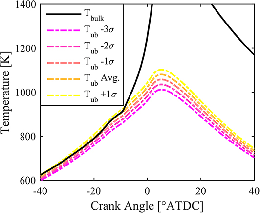
Figure 1. Unburned temperature profiles for various multiples of the standard deviation of temperature as a function of crank angle compared to the bulk gas temperature for an example case.

Predicting Autoignition Locations

The autoignition integral from Livengood and Wu (1954), shown in Equation (11) was used to predict the ignition locations of the various possible fuel mixtures along each thermal path defined in the previous section. Like the TSA method, the pressure is considered to be uniform throughout the combustion chamber. The fuel mixture properties, such as the premixed mass fraction, equivalence ratio, and EGR rate, and thermodynamic information, such as temperature and pressure, are known as functions of crank angle. With this information, the ignition delays for the fuel mixtures for each fuel and thermal zone can be determined by linear interpolation of a large look-up table of ignition delay values, or by use of an ignition delay correlation that covers the entire range of possible mixture compositions and thermodynamic conditions such as those in DelVescovo et al. (2016) and Chuahy et al. (2018). The ignition delays were determined at each crank angle step starting from the EOI timing. In reality, the premixed fuel autoignition integral should be computed starting from the IVC timing, however, the cumulative integral between IVC and EOI is very small ≪ 0.01, due to the very long ignition delays assocd EOI is very smalles of the early compression stroke, and is therefore ignored in this analysis.

$\begin{array}{ll}AI={\displaystyle {\int }_{t_0}^{t_{ign}}}\frac{1}{\tau }dt& (11)\end{array}$

The autoignition integral can then be computed for each thermal and fuel mixture zone according to Equation (11), starting from the EOI timing corresponding to t₀, until ignition when the cumulative integral equals 1.0. An example showing the trend of ignition delay and cumulative autoignition integral is shown in Figure S3 for 2 mixture compositions (designated by PRF number) where the premixed fuel is iso-octane (PRF100), and the DI fuel is n-heptane (PRF0). As temperature and pressure increases due to compression, the ignition delay decreases and the cumulative AI integral increases until the value of the AI integral reaches 1.0, thus defining the ignition location in crank angle space. In the example provided, the PRF100 case represents the premixed background fuel, while the enhanced reactivity of the PRF75 case includes both the chemical reactivity effect of n-heptane addition, as well as the mixture reactivity effect of the increased equivalence ratio according to the methodology presented in Section Initializing Zones.

Figure 2 shows the predicted autoignition crank angle locations for various thermal profiles as a function of PRF number for the same example case. As expected, as PRF number decreases, the ignition zone advances due to the higher reactivity of n-heptane compared to isooctane and the associated increase in equivalence ratio. Additionally, the colder zones autoignite later than the hotter zones. However, for a given crank angle, it is clear that multiple PRF blends may autoignite at the same instant depending on the thermal path of the fuel (e.g., a less chemically reactive fuel at a higher temperature may autoignite at the same crank angle as a more chemically reactive fuel at a lower temperature). This is an important consideration when attempting to determine the relative energy released by a particular zone, and thus a methodology must be developed in order to assign the energy release to the correct fuel blend. It should be noted that for an engine utilizing direct injection, in addition to variable thermodynamic conditions, the fuel/air composition is also constantly evolving due to mixture motion and mixing. In the present work, this mixing behavior is not considered, as the method is designed to predict a static fuel distribution, representing one of the fundamental limitations of the method. Thus, the range of applicability of the proposed methodology is explored in following sections.

FIGURE 2

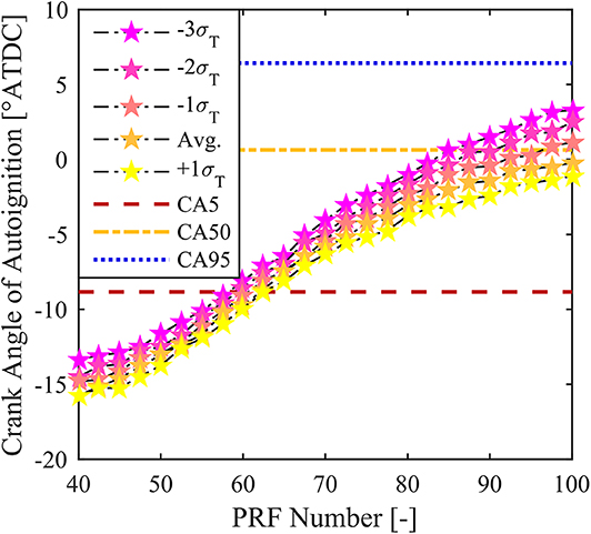
Figure 2. Predicted AI crank angle (indicated by stars) as a function of PRF number for various thermal profiles, with lines showing CA5 (red dashed), CA50 (yellow dash dotted), and CA95 (blue dotted).

Determining Probability Density Functions

With the autoignition locations of all the fuel mixture and thermal zones calculated, the next step in the analysis is to determine the distribution of mass responsible for the energy release. Like the TSA method, the FSA method uses the cumulative mass fraction burned (MFB) profile to distribute energy amongst the various fuel and thermal zones. The MFB profile is calculated by dividing the calculated cumulative heat release by its maximum value.

The autoignition crank angles belonging to the respective fuel and thermal zones were then grouped into crank angle windows, or “bins,” between CA5 and CA95. The analysis considers only energy released between CA5 and CA95, in order to eliminate the effect of the LTHR, and late cycle oxidation, respectively. The crank angle bins used in the analysis were 1.0 °CA wide. The bin width does not have a strong influence on the predicted fuel distribution as long as the bin width is greater than or equal to the resolution of the crank angle data. This resolution is typically 0.1-0.25 °CA. A bin width of 1.0 °CA eliminates some amount of uncertainty in the autoignition prediction, as the typical accuracy of Livengood-Wu autoignition predictions compared to SI and HCCI ignition events is typically on the order of 1-2 °CA (Swan et al., 2006; Shahbakhti et al., 2007; Kalghatgi et al., 2015; DelVescovo et al., 2016).

This binning process is represented in Figure 3, where the green region represents the bin of interest. The energy released within the window was determined by subtracting the value of the MFB at the right edge of the bin from the value of the MFB at the left edge of the bin, thus representing the fraction of mass consumed during this window. The minimum possible fuel blend (i.e., premixed fraction or PRF number) was defined by eliminating any premixed fuel zones on the highest temperature path (+1σ path) with autoignition predicted before the crank angle corresponding to CA5. This is justified by the fact that if this fuel blend existed, then there would have been a corresponding heat release associated with its autoignition at the most reactive (highest temperature) condition. Since it was assumed that fuel is equally likely to be “hot” as to be “cold,” this implies that any fuel mixture that autoignites along the hottest possible path before CA5 is not possible or present at the time of combustion. For the example shown in Figure 3, this methodology implies that fuels blends less than PRF62.5 are not present in the mixture at the time of combustion. The maximum possible premixed fraction is defined in a similar manner, except that the coldest thermal path (−3σ) is considered, and if a premixed zone does not autoignite before CA95, then this zone either does not exist or remains unburned throughout the cycle. From Figure 3 it can be seen that for this case, all fuels blends up to PRF100 are possible. Fuel that was outside the minimum and maximum possible premixed fraction was not considered to exist in the analysis, and the mass attributed to the autoignition of these blends was set to zero.

FIGURE 3

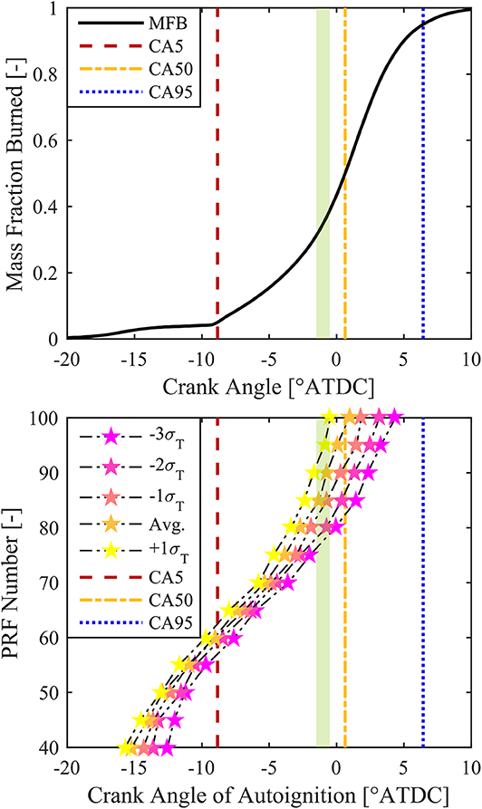
Figure 3. Graphical representation of the binning process by which autoignition zones for various PRF numbers and temperature paths were compared to the mass-fraction burned profile. The green region represents an example 1.0°CA wide bin.

If there is overlap among thermal zones within a given crank angle window, then the corresponding energy within this window was distributed according to breakdown shown in Figure 4. The cumulative distribution shown is from a non-reacting CFD simulation of a representative HCCI combustion case. If all thermal zones are represented within a crank angle bin, then 80% of the energy is distributed into the fuel mixture zone at the mean thermal path, 5% is distributed to the +1σ thermal path fuel mixture, 12% to the −1σ thermal path, etc. If there is no overlap, and only one zone is accounted for in the crank angle bin, then all the energy is assumed to belong to the fuel mixture zone that ignites in the bin. This approach assumes that the natural thermal stratification present in a homogeneous charge simulation is representative of the thermal distribution in a stratified fuel approach, not accounting for the effect of spray vaporization on the temperature distribution, which is handled separately. This approach served as a way in which to determine the relative weighting of a given thermal pathway, in order to distribute the energy associated with a given crank angle bin into the appropriate fuel mixture zones. The energy for each fuel mixture zone could then be summed across all the thermal paths, establishing the cumulative density function of energy as a function of premixed fraction. One important consideration is that this methodology only accounts for fuel that actually burns, so to approximate the fraction of the total fuel accounted for by the analysis, this cumulative density function was multiplied by the combustion efficiency (η_comb).

FIGURE 4

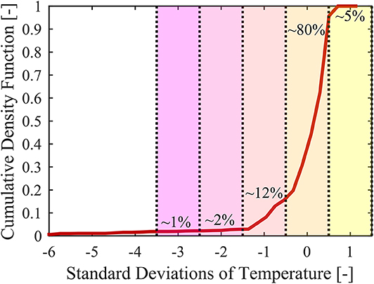
Figure 4. Cumulative density function of temperature normalized by standard deviation (red line), showing the relative distribution of temperature among “thermal zones” denoted by colors.

In order to convert from the cumulative density function of energy to fuel-mass density, the energy fraction of each premixed zone, (ef_i) was multiplied by the average mixture LHV divided by the zone lower heating value (LHV_i) as shown in Equation (12). This is an important manipulation as, for a given fuel mass, a fuel mixture with a high lower heating value will release more energy than a fuel with a low lower heating value, yet would account for the same total fuel mass. This is not a consideration that has to be made in a single fuel strategy, or in a homogeneous charge strategy. A similar manipulation must be made to convert from the cumulative density of energy to cylinder-mass density. As shown in Equation (13), the energy fraction of each premixed zone was multiplied by the average energy density, which is equivalent to the fuel energy (Q_fuel) divided by the trapped mass (m_trap), and divided by the zone energy density (E_i). This is necessary because a unit of cylinder mass at a given local equivalence ratio has a very different quantity of energy depending on the equivalence ratio, i.e., a unit of total mass at φ of 0.25 contains much less fuel-energy than a unit of total mass at φ of 1.0. This again is not a consideration that needs to be made for homogenous charge strategies, but is important for stratified approaches.

$\begin{array}{ll}m{f}_i=e{f}_i\frac{LH{V}_{avg}}{LH{V}_i}& (12)\end{array}$

$\begin{array}{ll}{m}_i=e{f}_i\frac{\left(\frac{Q_{fuel}}{m_{trap}}\right)}{E_i}& (13)\end{array}$

The cumulative density functions for energy, fuel-mass, and total-mass are the cumulative sums of the respective fraction. Each respective PDF can be calculated according to Equation (14), where the x-variable is the variable of interest, e.g., PRE, PRF number, φ, temperature, etc. The premixed mass fraction and PRF number are fuel-mass weighted quantities, and temperature and equivalence ratio are total-mass weighted quantities. The expected value can then be calculated from the PDF according to Equation (15), and compared to the average value to determine the relative error of the methodology.

$\begin{array}{ll}PDF=\frac{dCDF}{dx}& (14)\end{array}$

$\begin{array}{ll}Exp[x]={\displaystyle {\int }_{-\infty }^{+\infty }}x*PDF(x)dx& (15)\end{array}$

FSA Method Assumptions

Like the TSA method, there are a number of implicit and explicit assumptions associated with the FSA method. These assumptions are summarized as follows:

• The pressure is uniform in the cylinder.

• The premixed fuel, air, residuals, and EGR are completely mixed at IVC.

• Chemical reaction rates are very fast relative to engine time scales, and therefore when a zone autoignites it does so instantaneously.

• There is no heat or mass transfer between zones, implying that the hot burned gases do not mix with cold unburned gases, and in turn, accelerate the autoignition events.

• There is no flame propagation in the combustion chamber, which would cause zones to burn prior to the autoignition integral prediction.

• Fuel instantaneous vaporizes at the end of injection.

Results

In order to validate the FSA model, reacting and non-reacting CFD simulations were performed with KIVA3V release 2 (Amsden, 1999). The reacting simulations were used to validate the CFD simulations against experimental HCCI and RCCI data from DelVescovo et al. (2016) and DelVescovo et al. (2017), respectively. Non-reacting simulations were used to generate PDFs of fuel distributions for various injection timings and initial conditions to compare to the FSA results. The two approaches were able to provide a direct comparison with the FSA method, as the non-reacting fuel distributions could be compared to the FSA results using the reacting pressure and heat release data, thus providing a known distribution of fuel and a known result to determine the validity of the FSA methodology, provided the chemical mechanism used in the CFD and CV ignition delay simulations were equivalent.

CFD Modeling Setup and Submodels

A list of the improved sub-models coupled to the KIVA3V code and utilized in this work are shown in Table 1, in addition to the spray model constants used for the KH-RT spray breakup model, and GASJET near nozzle flow model. As it is not the focus of the present work, a detailed description of the simulation models is omitted here. Significantly more detail regarding the computational models and methodology can be found in the appropriate references as well as in Dempsey (2013) and Kokjohn (2012), and additional validation of the performance of the CFD code and spray model parameters used in this work can be found in Chuahy and Kokjohn (2017). With the exception of the KH breakup decay timescale, which was taken from Dempsey (2013) for his work on the same engine platform, and the GASJET entrainment constant from Perini and Reitz (2016), the values shown in the table are those recommended by the respective model authors.

TABLE 1

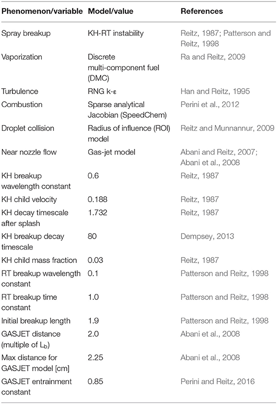
Table 1. Sub-models and spray model constants used in CFD simulations.

A reduced chemical mechanism developed by Wang et al. (2013) with 71 species and 360 reactions, developed to model the combustion and polyaromatic hydrocarbon formation for diesel and n-heptane/toluene mixtures, was used for the present work. The mechanism was validated with experimental shock tube data, premixed flame species concentration profiles, HCCI engine experiments, and direct injection constant volume spray experiments. The iso-octane portion of the reduced ERC PRF mechanism from Ra and Reitz (2008) (9 additional species and 11 reactions) was present in the mechanism files from Wang et al. (2013), and was enabled for the purposes of this work. This mechanism was chosen as it performed very well for PRF fuels in HCCI and RCCI combustion CFD simulations, with very minimal modifications to the experimental operating conditions (typically well within the experimental uncertainty), as shown in following sections.

Figure S5 in the supplementary materials shows the computational sector mesh used to model the Caterpillar SCOTE stock piston bowl used in the HCCI and RCCI experiments presented in DelVescovo et al. (2016, 2017), while the engine geometry, thermal boundary conditions, and direct injector parameters are presented in Table 2. The sector mesh was used in order to reduce simulation times and the total number of cells, and a periodic boundary condition was established on the sector faces. The squish height was increased slightly from the production piston profile in order to match the compression ratio, accounting for the lack of valve recesses and volume around the injector body in the mesh. The relatively coarse mesh was comprised of about 10,800 cells, and average reacting simulation times were on the order of 6–8 h. Only the closed-cycle portion of the engine cycle could be simulated due to the lack of intake and exhaust runners and valves in the mesh setup. Additionally, constant wall temperatures were applied as thermal boundary conditions in the simulations. These temperatures varied depending on the nature of the boundary as shown in Table 2. The values were optimized by matching simulated motored engine data to experimental “hot” motoring traces taken immediately after running with the engine at operating temperature.

TABLE 2

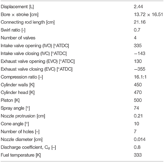
Table 2. Stock Caterpillar 3401E SCOTE engine geometry, thermal boundary conditions, and direct-injector parameters used in CFD simulations.

The injection rate was approximated by a trapezoidal shape with a closing rate that was twice as fast as the opening rate. This was approximated by qualitatively assessing the measured rate of injection (ROI) profiles in Dempsey (2013), for the same model injector body and injector tip used in the experiments. The injection velocities, which serve as the input to KIVA, were computed by assuming a constant opening and closing rate that is a function of injection pressure, and calculating the duration of the injection required to provide the appropriate quantity of fuel based on the rate shape constraints. The initial slope of the injection rate was set by qualitatively matching the bulk heat release characteristics for a late injection RCCI case (−20°SOI), where the influence of injection rate is the greatest as the mixing process controls the rate of heat release. The remaining injector parameters used to model the Bosch 7 hole 141 μm CRI2 injector used in the experiments are summarized in Table 2. A constant injector delay of 0.32 ms, which is equivalent to 2.5 °CA at 1300 rev/min engine speed, between the commanded SOI and the actual SOI was used for all simulations. This value comes from Bosch-type rate of injection bench data from Dempsey (2013), and was shown to be independent of injection duration and rail pressure.

CFD Validation With Experimental Engine Data

The CFD model was first validated against HCCI engine data from DelVescovo et al. (2016) taken on the heavy-duty Caterpillar SCOTE platform, with the geometry shown in Table 2. The simulations were performed with the 3-D mesh shown in Figure S4, and the reactants were assumed to be completely premixed and uniform in composition. A constant residual fraction of 4% was assumed for all operating conditions, and the reactants were composed of fuel (iso-octane and n-heptane), air (O₂ and N₂), and residuals, which were assumed to be the products of complete combustion (CO₂, H₂O, O₂, and N₂). The reactant composition was calculated from the fuel mass, IVC conditions (assuming ideal gas law to determine number of moles of mixture at IVC), and the global fuel blend. The IVC temperature was adjusted up or down slightly from the experimentally calculated IVC temperature for these comparisons, effectively acting as a chemical kinetics tuning parameter.

The experimental IVC temperature was calculated by using the relationship outlined by Yun and Mirsky (1974), which assumes an isentropic process during the gas exchange processes to determine the fraction of residual gases at IVC. The remaining initial conditions were taken directly from the time-averaged experimental values. A summary of the experimental operating conditions is shown in Table 3, and the approximate uncertainties for the experimental measurements are shown in Table 4. While each measured value has some amount of uncertainty, the magnitude of the uncertainties are much less than the uncertainty in the IVC temperature and mixture homogeneity, therefore for the purposes of the CFD simulations these uncertainties were ignored.

TABLE 3

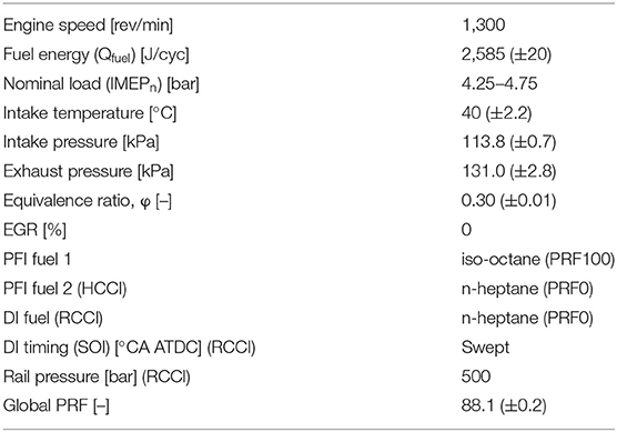
Table 3. Engine operating conditions of PRF HCCI and RCCI experiments.

TABLE 4

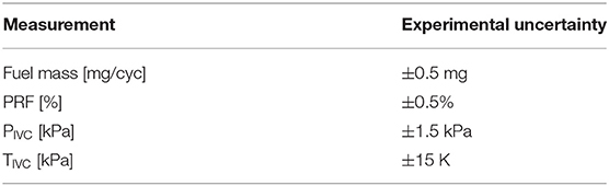
Table 4. Approximate experimental measurement uncertainties.

The initial conditions provided to the CFD simulations for the HCCI validation cases are listed in Table S1, while Figure S5 shows the ensemble-averaged pressure and heat release traces for the HCCI experimental data in black overlaid on the region of ±1σ in gray, with the CFD predictions plotted in red dotted lines. The differences between the calculated IVC temperatures and the IVC temperatures required in the simulations were between +4 and +8 K, which is well within the expected uncertainty of the experimental measurements. Additionally, variations between the simulated and experimental residual composition, charge stratification, and heat transfer, could easily be responsible for the range of IVC temperature adjustment required in the simulations. In general, the simulations do an excellent job of predicting HCCI combustion behavior at the simulated conditions. Additional validation simulations were performed with the same fuel energy input but varying intake conditions, but were omitted here for brevity. The results of these additional simulations showed similar performance to those presented, with required IVC temperature adjustment between −2 and +11 K.

With the CFD model showing good agreement with HCCI engine data with the chosen chemical mechanism, the model was evaluated against PRF RCCI engine data from DelVescovo et al. (2017) in order to assess its performance under RCCI conditions using premixed iso-octane and direct injected n-heptane for various direct injection timings and intake conditions. The reactant composition was calculated as described in the previous section for the HCCI simulations, with the exception that only the iso-octane was premixed. The IVC temperature was again used as a tuning parameter for the global chemical kinetics to match the combustion phasing of the simulations relative to the experiments.

A summary of the experimental operating conditions for the experimental RCCI data is also shown in Table 3, and the initial conditions of the CFD simulations for the cases are listed in Table S2. In this case, the PRF number refers to the percentage of total fuel that is premixed (i.e., 88% premixed iso-octane, 12% direct injected n-heptane). As shown in Table S2, the IVC temperature adjustment required to match combustion phasing between the experiments and simulations ranged between −1 and +12K, which is well within the estimated experimental uncertainty for this parameter. Figures S6, S7 in the supplementary materials show the experimental and calculated pressure and heat release rates for the early SOI timing cases between −140° and −45°, and for the late injection timing cases between −40° and −17°, respectively. Similar to the previous section, the ensemble-averaged pressure and heat release traces for the experimental data are shown in black overlaid on the region of ±1σ in gray, while the CFD predictions are plotted in red dotted lines.

For the earliest SOI case (−140°), the simulation over-predicted the mixing of the direct injected fuel, and therefore resulted in a shorter combustion duration than observed experimentally, while for the late injection timing cases, particularly −20° and −17° SOI, the two-stage combustion event seen in the experiment was not captured particularly well in the CFD simulations, and the general trends in combustion for these two cases were not as well-captured as earlier SOI timings. Despite these discrepancies, exceptionally good agreement is seen in the pressure and heat release comparisons between the experimental and simulated results between injection timings of −90° and −30°. This injection timing range is the typical range of interest for RCCI combustion (Kokjohn, 2012), thus providing confidence in the simulation results and trends for RCCI.

Validation of FSA Method With Non-reacting CFD

Given the success of the reacting CFD simulations in matching experimental HCCI and RCCI pressure and heat release rate data, non-reacting CFD simulations using the same numerical model presented in the previous section were used to validate the FSA method. The CFD simulations were used to determine the extent of the natural thermal stratification, and as a comparison between the FSA predicted fuel distribution and the known fuel distribution provided by the CFD result. The reacting CFD pressure, temperature, and mass fraction burned profiles were used as input conditions in the FSA analysis to predict ignition locations and the representative fuel distribution. The cell information from the CFD simulations were used to generate PDF and CDF profiles with bins at every 2.5 PRF number between 0 and 100, thus providing a direct comparison between the FSA and CFD results, since the fuel distribution in the CFD simulations yields the CFD pressure and HRR trace, and working backwards, the reacting pressure and HRR trace should return the fuel distribution using the FSA method. Assuming the FSA method could recover the global averaged PRF number, φ, and fuel distribution profile, the methodology was assumed to be applicable.

One of the inputs of the FSA method is the standard deviation of temperature (σ_T) at some arbitrary crank angle (CA_arb). This parameter defines the various thermal profiles which may exist in the cylinder. This parameter was determined from non-reacting CFD results by analyzing the development of the cell temperatures as a function of crank angle. The standard deviation was calculated from the cell temperatures weighted by cell mass at each crank angle; as the mass-averaged cylinder temperature increased due to compression, so too did the standard deviation of temperature. Mass-weighted PDFs of temperature were also calculated at each crank angle, showing the evolution of the relative distribution of temperature over time. Figure 5 shows the evolution of the mass-averaged temperature profile as a function of crank angle for three representative cases, one HCCI case, and two RCCI cases with different SOI timings. The second peak that starts to define itself around −15 °CA in the HCCI case is a result of heat transfer in the squish region. This bimodal distribution would likely not present itself with a flat-top piston geometry. The long tail of the distribution extending to low temperatures is a result of the crevice region, where heat transfer to the piston and cylinder walls keeps the cell temperatures low. In general, the temperature distributions, standard deviation, and average bulk gas temperature are largely unaffected by the SOI timing, though in the −20° SOI case, the effect of the vaporization process can be clearly seen as the range of cell temperatures at −15 °CA, which occurs during the injection event, extends downwards significantly due to the injection and subsequent vaporization of the cool fuel. After the end of injection, this seems to have little effect on the temperature distributions, however. This result implies that the evaporative cooling induced by the direct-injected fuel has much less effect on the temperature distribution than the natural thermal stratification, even for a relatively large bore engine in this case.

FIGURE 5

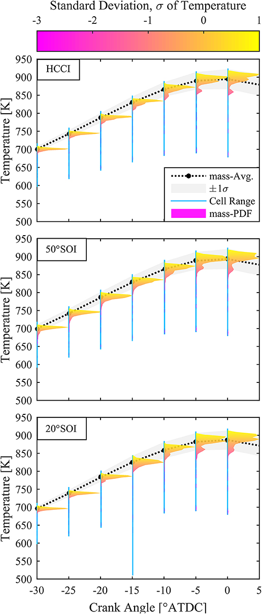
Figure 5. Temperature evolution as a function of crank angle for representative HCCI (Top) and RCCI cases with SOI of −50° (Middle) and SOI of −20° (Bottom), with the mass-weighted PDF of temperature colored by multiple of σ.

The standard deviation of temperature parameter (σ_T), which is effectively a measure of the magnitude of thermal stratification, was plotted for various SOI timings as a function of crank angle for the non-reacting CFD simulations. Figure S8 in the supplementary material shows the result of these simulations for various injection timings. The SOI timing initially influences the temperature distribution, but by around −10 °CA and beyond, the effect of the SOI timing on the thermal stratification is largely absent. This analysis led to −10 °CA being chosen as the arbitrary crank angle at which to match the temperature profiles, with a σ_T of 21 K. This crank angle was chosen because it was close to the start of combustion for the various cases tested in the validations shown here, and because as shown in Figure S8, the standard deviation at this crank angle was largely independent of SOI within the range of conditions tested in the experiments and CFD modeling for RCCI combustion.

Using the effective polytropic coefficient method outlined in section Accounting for Thermal Stratification, the various thermal paths could be calculated for the non-reacting case to examine the agreement between the calculated thermal paths using just the polytropic coefficients, and the CFD predictions, which include a full heat transfer model. The result of this comparison is shown in Figure 6. Early in the compression stroke, heat is transferred from the relatively hot cylinder walls and piston surfaces into the combustion chamber. After the chamber gas exceeds the temperature of the walls and piston surfaces due to compression, heat is transferred in the opposite direction back into the walls, and piston surfaces. This heat transfer process leads to the discrepancies seen between the polytropic processes defined by the effective γ values, and the CFD predicted temperature paths. The polytropic processes match the in-cylinder temperatures at the IVC condition, and at the arbitrary crank angle defined (in this case −10 °CA). As would be expected, it was found to be most important to match the temperature distribution near the start of combustion in order to accurately predict the autoigntion locations of the various fuel mixture zones. It is clear from Figure 6, however, that a better methodology for determining the various thermal paths in the cylinder is needed to more accurately match the thermal trajectories of the charge. Multizonal temperature approaches, such as those employed by Fiveland and Assanis (2001), and Komninos et al. (2004), may provide an improved temperature prediction methodology, and could help the predictive ability of the FSA method beyond what is presented in this work.

FIGURE 6

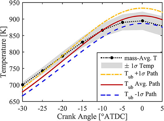
Figure 6. CFD predicted temperature (black) with ±1σ region (gray) as a function of crank angle. Also plotted are the polytropic average temperature path (red), +1σ path (yellow), and −1σ path (blue) as functions of crank angle.

The ignition locations corresponding to the various thermal and compositional paths were predicted by linearly interpolating a large 5-D matrix of ignition delay values simulated with the Cantera package in MATLAB using the approach described in DelVescovo et al. (2016). The 5-dimensions of the matrix corresponded to temperature, pressure, EGR rate, equivalence ratio, and the mass ratio of fuel one to total fuel. For these validation cases, fuel 1 was isooctane, and fuel 2 was n-heptane. The same reduced chemical mechanism used in the 3-D CFD simulations shown in section CFD Validation with Experimental Engine Data (Wang et al., 2013) was used to simulate the ignition delays of the fuels.

Another consideration regarding the proposed FSA methodology is that the method predicts only a static distribution that effectively corresponds to the fuel distribution at the start of combustion. In reality, the fuel distribution in the CFD simulations, and in a real engine, is constantly evolving due to the effects of turbulent mixing and swirl. The evolution of the fuel distribution as a function of crank angle for two different SOI timings in RCCI CFD simulations can be clearly seen in Figure 7. As the amount of time after injection increases, the fuel/air mixture trends toward homogeneity. In order to compare the FSA method result and the CFD predictions, a crank angle needs to be defined at which to determine the CFD predicted fuel distribution. Since the FSA method predicts the fuel distribution at the start of combustion, a crank angle near the beginning of the combustion process was chosen for each individual case. The crank angle chosen was the crank angle closest to the approximate start of combustion that had been outputted for post-processing.

FIGURE 7

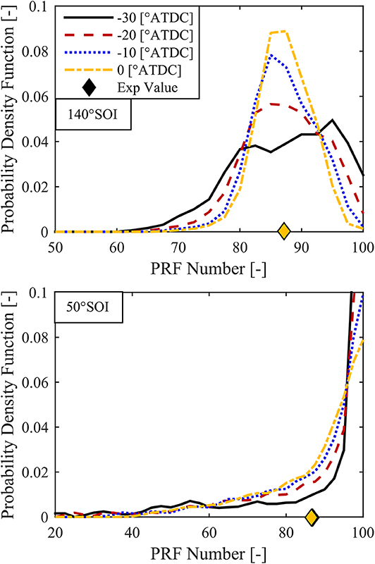
Figure 7. PDFs of PRF number for two SOI cases, −140° SOI (Top), and −50° SOI (Bottom), for various crank angles, showing the mixing of the fuel over time.

Because the FSA method cannot account for unburned fuel, and because of differences between the actual fuel chemistry and the assumed sequential autoignition, e.g., energy released due to late cycle CO oxidation, the maximum value of the cumulative density function determined from the FSA method was always <1. The missing mass could be accounted for in a number of ways, including assuming that the mass belonged to the 100% premixed fuel zone, as this zone is the least likely to ignite, and most likely to be trapped in the crevice regions. The missing mass could also be assumed to be equally likely to belong to any possible zone. This involves the normalization of the CDF by its maximum value. Figure 8 shows at the top, the non-normalized result of the FSA method compared to a non-reacting CFD simulation for an RCCI case with a −140 °SOI. The non-normalized FSA method only accounts for ~96% of the total fuel mass. Because the CDF does not reach 1.0, and thus does not account for all fuel mass present, the expected value (red diamond) cannot be compared directly to the actual value (black diamond), whereas the normalized FSA result shown below accounts for all available fuel mass (by definition), and the expected value matches the actual value.

FIGURE 8

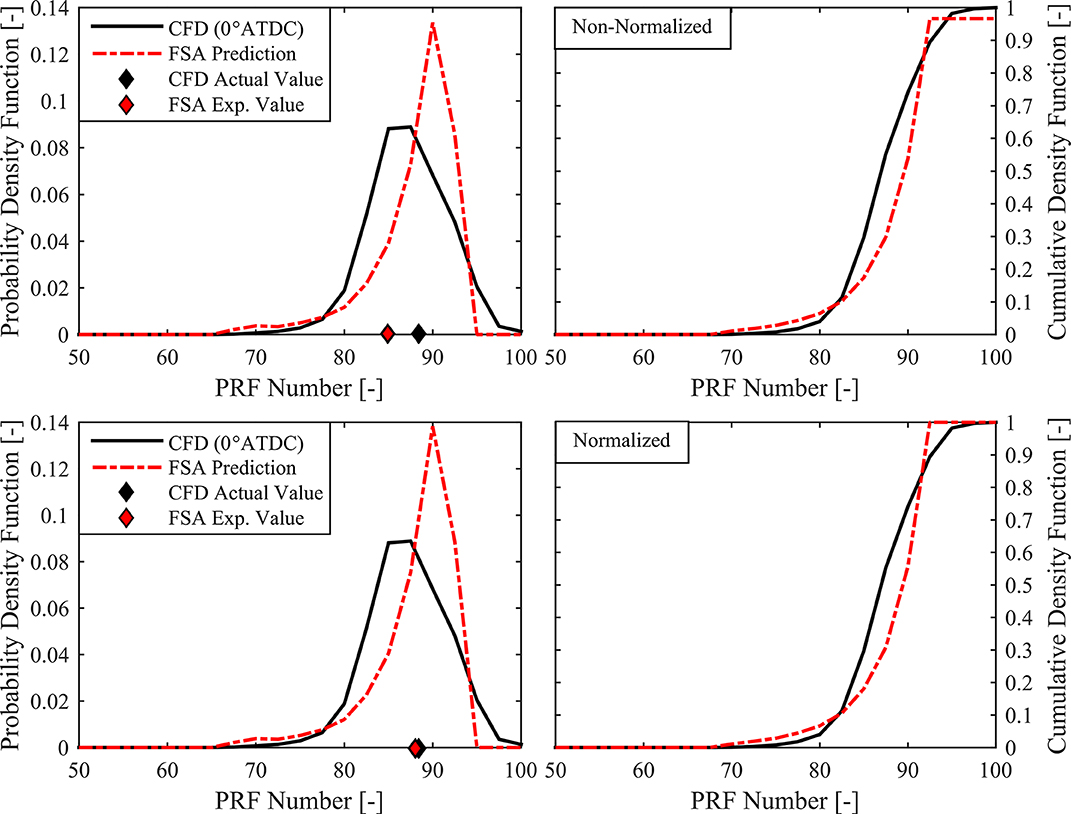
Figure 8. PDF (Left) and CDF (Right) vs. PRF Number for non-reacting CFD at 0 °CA for −140° SOI case, compared to non-normalized FSA method result (Top), and normalized FSA method result (Bottom).

Figure 9 shows at the top, the non-normalized FSA method result compared to the non-reacting CFD fuel distribution for an RCCI case with a −30° SOI. Here the FSA method is only able to account for about ~65% of the total fuel mass, though the general shape of the distribution, except for the very large quantity of unmixed PRF100, is well-captured. For this late injection timing case, the FSA method assumptions start to break down. Normalizing the distribution, as seen in the figure at the bottom, does not improve the FSA prediction, and the expected value is not able to recover the global averaged value of PRF. While it may be more appropriate to assume that the unaccounted for mass in these late SOI cases was premixed fuel, this assumption would have to be made a posteriori, thereby diminishing the predictive capability of the methodology. Thus, in this work, all the CDFs shown were normalized by their maximum value. The approach taken for the validation cases was to normalize the FSA predicted distribution and adjust the IVC temperature up or down to recover the global averaged premixed mass fraction and equivalence ratio. Late injection timing cases were never able to recover the global average values, and therefore are assumed to have violated one or more of the inherent assumptions of the FSA method, namely, that there is no flame propagation, or the instantaneous vaporization at EOI stipulation. Therefore, mixing limited combustion cases are not well-suited for the proposed methodology given that the methodology is only capable of predicting a static fuel distribution at the start of combustion, thus, injection timings which lead to significant fuel/air mixing during the combustion process are not well-captured.

FIGURE 9

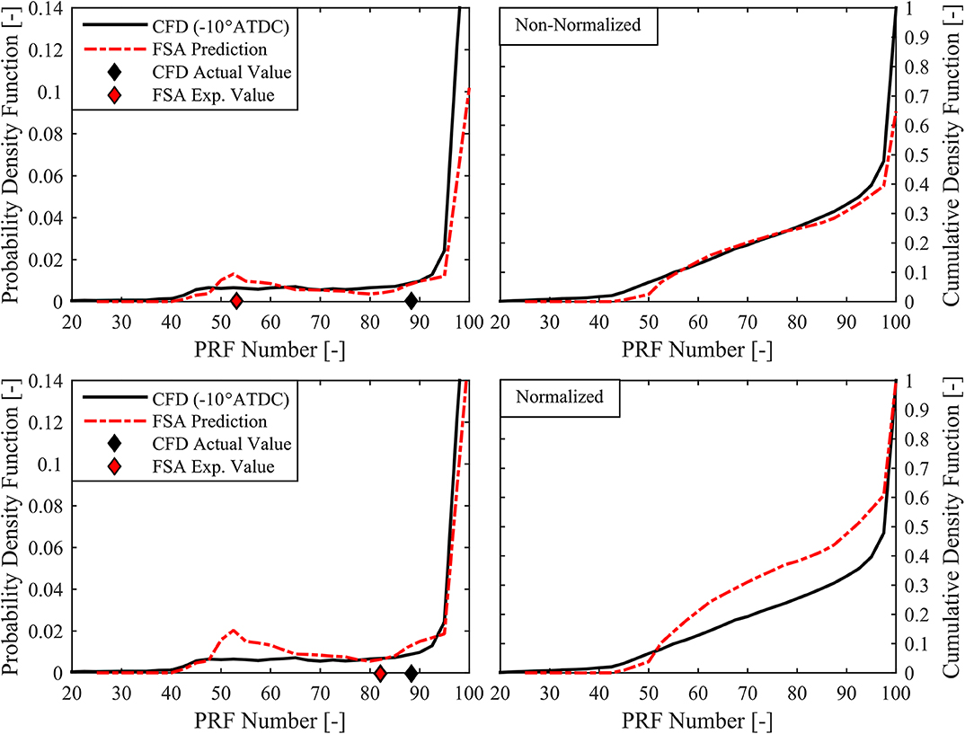
Figure 9. PDF (Left) and CDF (Right) vs. PRF Number for non-reacting CFD at 0°CA for −30° SOI case, compared to non-normalized FSA method result (Top), and normalized FSA method result (Bottom).

The validated PRF RCCI cases with fixed global PRF as well as an HCCI case with a similar global PRF number from Section CFD Validation with Experimental Engine Data were used as the validation cases for the FSA analysis. The CFD pressure and MFB traces served as inputs for the FSA method to predict the fuel distribution. The non-reacting CFD simulations served to validate the corresponding FSA predicted fuel distributions. Figures 10, 11 show the FSA method results compared to the CFD-predicted fuel distributions for the various SOI timings, and the one HCCI case presented here. In general, very good agreement is seen between the CFD and FSA method results between SOI timings of −140° and about −35°, at which point the predictions begin to deviate significantly, likely due to the violation of one or more of the inherent assumptions of the methodology. The HCCI case with no fuel stratification shows reasonable agreement between the FSA method and CFD predictions, though despite the minor amount of fuel stratification predicted by the CFD result for the −140°SOI case, the reacting CFD pressure and heat release for the HCCI and −140°SOI case are nearly identical. The result of this validation shows that the FSA method is able to provide relatively good agreement between the predicted and actual fuel distributions from CFD simulations within the range of injection timings of interest in RCCI combustion (−140° to about −35° ATDC). This injection timing range corresponds directly to the kinetically controlled combustion regime, characterized by advanced combustion phasing with retarded injection timing. Beyond −35° ATDC SOI timing, the combustion regime transitions toward a mixing limited regime characterized by retarded combustion phasing with further injection timing retard (DelVescovo et al., 2017).

FIGURE 10

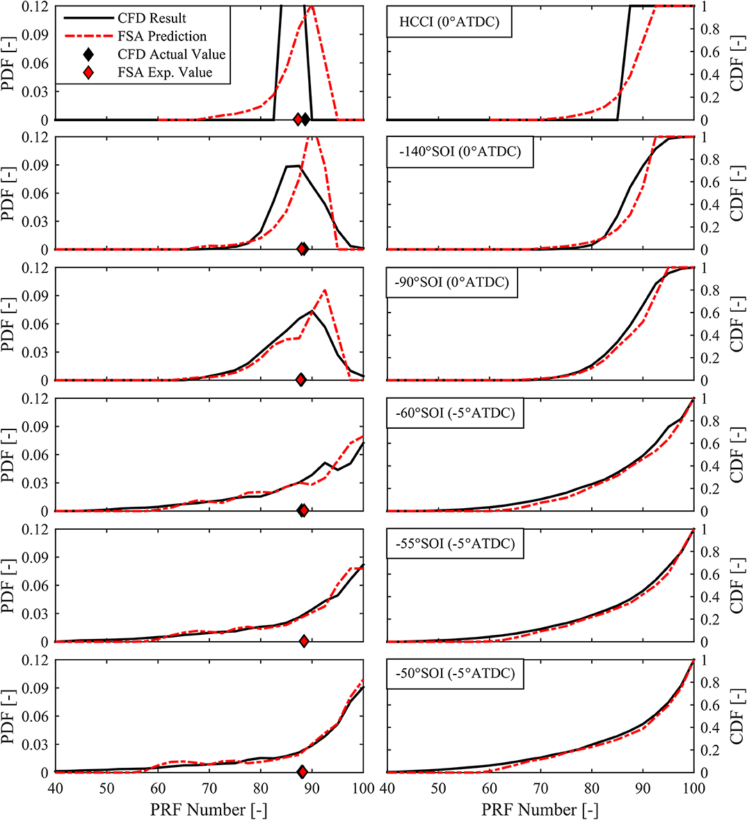
Figure 10. PDFs (Left) and CDFs (Right) vs. PRF Number for non-reacting CFD at specified crank angle for specified SOI case from HCCI to −50°, compared to normalized FSA method predicted results.

FIGURE 11

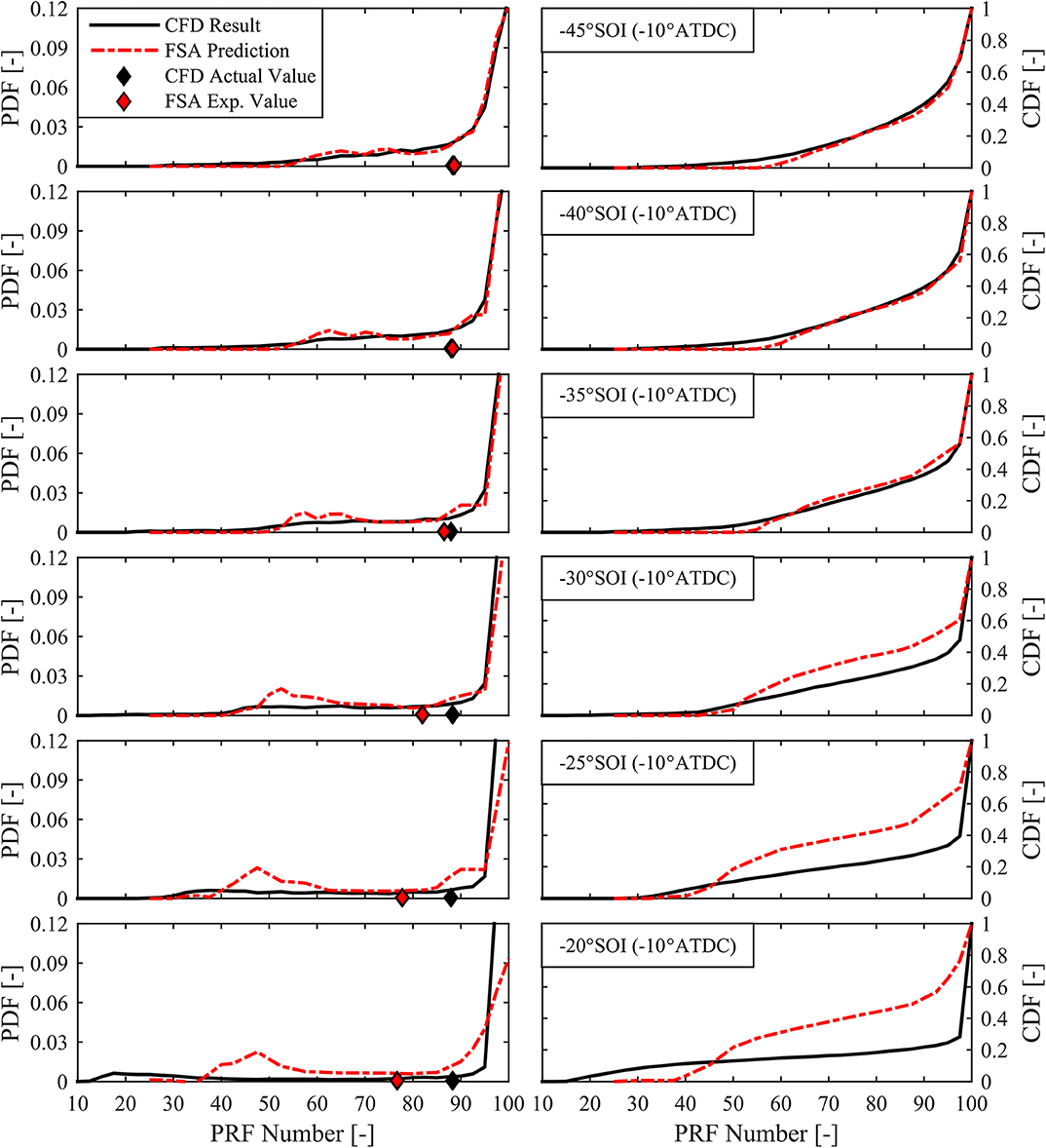
Figure 11. PDFs (Left) and CDFs (Right) vs. PRF Number for non-reacting CFD at specified crank angle for specified SOI case from −45° to −20°, compared to normalized FSA method predicted results.

Discussion

The validation presented in the previous section showed generally good agreement between the FSA predicted fuel stratification and fuel distributions generated with non-reacting CFD simulations within the range of SOI timings of interest to RCCI combustion for the tested cases. While the current work presents only a single engine operating condition with no EGR, the methodology proposed could be generally applied to any kinetically controlled engine operating condition or combustion strategy, including single fuel strategies such as PFS, PPC, or GCI, and cases with and without EGR. Given the validity of the approach, what follows here is a discussion of the possible applications of the FSA methodology. The FSA approach can be used in two distinct ways; first, as a post-processing tool to analyze the distribution of fuel reactivity and equivalence ratio from experimental results, and the second as a pre-processing tool to determine, given a desired heat release profile and fuel chemistry, the required fuel distribution. While the first approach may yield valuable information regarding the distribution of direct-injected fuel at the start of combustion, particularly with respect to general trends in emissions such as NO_x and soot, the second approach is potentially more impactful. For example, the FSA method could be used to predict fuel stratification requirements for favorable heat release rate profiles. The heat release rate could be constrained by some operational limitations such as maximum PPRR, maximum peak pressure, or can simply be the optimized heat release for gross efficiency. The heat release could have some predefined shape defined by a mathematical function such as a Gaussian distribution, or Wiebe function, or some arbitrary profile, and the FSA method would then predict the necessary fuel distribution, based on the initial conditions and chosen fuel chemistry.

Using the FSA method, the effect of the premixed and direct-injected fuel chemistry on the fuel stratification requirements could also be explored. Assuming some optimal HRR at given initial conditions, the stratification requirements for any combination of premixed and direct-injected fuel could be predicted. Using this method the user would be able to gain significant insight into the optimization of alternative fuels in a kinetically-controlled, stratified-charge strategy. Alternatively, the FSA method could be used to determine stratification requirements for varying engine operating conditions, or be used to determine boost/dilution requirements given some desirable heat release profile and fuel distribution. The method does, however, require the fuel chemical kinetics to be well-characterized, and unfortunately does not provide any information regarding how to actually achieve the required fuel distribution. However, by coupling the proposed methodology with a 1-D spray model, or using a genetic algorithm coupled to a non-reacting 3-D CFD code, a user may be able to determine the direct injection schedule necessary to achieve the required fuel stratification conditions without costly combustion simulations or experiments.

Conclusions

In this work a 0-D methodology was developed to predict the fuel stratification necessary to achieve a certain heat release profile in stratified-charge, kinetically-controlled combustion strategies. The model was inspired by the Thermal Stratification Analysis (TSA) tool developed by Lawler et al. (2012, 2014a), which predicts in-cylinder thermal stratification in HCCI combustion events at the start of combustion, based on autoignition predictions, and experimental mass fraction burned data. The Fuel Stratification Analysis method utilizes a similar approach to predict the distribution of fuel in the cylinder at the start of combustion. Autoignition predictions are performed with the Livengood-Wu autoignition integral for various possible fuel mixtures, and associated equivalence ratios, for many possible thermal pathways in the cylinder. These autoignition predictions are then related to the energy released during specific crank angle windows, and probability density functions of the fuel distribution are calculated.

The proposed FSA methodology was validated via a two-step approach. First, 3-D CFD simulations were performed with KIVA3Vr2, and validated against experimental HCCI and RCCI engine data with various PRF blends. The CFD model showed good agreement with the experimental HCCI pressure and heat release traces with minimal adjustments to the IVC temperature calculated in the experimental results, but all cases were within the range of uncertainty of the experimental IVC temperature calculation. Relative to the RCCI combustion with fixed global PRF number, the CFD predictions demonstrated excellent agreement between SOI timings of −90 and −30 °ATDC, which is the range of interest in typical RCCI combustion, however injection timings outside of this range were not as well-captured. The second step in the FSA method validation procedure was to utilize non-reacting CFD simulations to generate the predicted fuel distributions present in the validated simulations. These fuel distributions were then compared to the distributions predicted by the FSA methodology using the reacting CFD pressure and heat release results as inputs. Various SOI timings, along with an HCCI case with PRF fuels were used as validation for the methodology. In general, good agreement was seen between the non-reacting CFD fuel distributions and the FSA method results between SOI timings of −140 and about −35 °ATDC. After this point, the FSA predictions and CFD results began to deviate significantly, indicating a violation of one or more of the inherent assumptions of the FSA methodology, and potentially indicating a transition into a mixing-limited combustion regime, or a regime in which significant flame propagation exists. Even the HCCI case with no fuel stratification showed reasonable agreement when the FSA method was applied.

Data Availability Statement

The datasets generated for this study are available on request to the corresponding author.

Author Contributions

DD, SK, and RR contributed to the conception and design of the study and the presented methodology. DD performed the experiments, developed the methodology, performed the computational simulations, and authored the first draft of the manuscript. All authors contributed to manuscript revision, read, and approved the submitted version.

Funding

This work was funded by the Office of Naval Research (ONR) under Grant No. N00014-14-1-0695.

Conflict of Interest

The authors declare that the research was conducted in the absence of any commercial or financial relationships that could be construed as a potential conflict of interest.

Supplementary Material

The Supplementary Material for this article can be found online at: https://www.frontiersin.org/articles/10.3389/fmech.2020.00028/full#supplementary-material

References

Abani, N., Kokjohn, S., Park, S. W., Bergin, M., Munnannur, A., Ning, W., et al. (2008). “An improved spray model for reducing numerical parameter dependencies in diesel engine CFD simulations,” in SAE Technical Paper 2008-01-0970 (Detroit, MI: SAE International). doi: 10.4271/2008-01-0970

CrossRef Full Text | Google Scholar

Abani, N., and Reitz, R. D. (2007). Unsteady turbulent round jets and vortex motion. Phys. Fluids 19:125102. doi: 10.1063/1.2821910

CrossRef Full Text | Google Scholar

Amsden, A. A. (1999). KIVA-3V, Release 2. Improvements to KIVA-3V. LA-UR-99-915. Los Alamos National Laboratory. Available online at: https://www.lanl.gov/projects/feynman-center/deploying-innovation/intellectual-property/software-tools/kiva/_assets/docs/KIVA3V.pdf

Google Scholar

Bakker, P. C., De Abreu Goes, J. E., Somers, L. M. T., and Johansson, B. H. (2014). “Characterization of low load PPC operation using RON70 Fuels,” in SAE Technical Paper 2014-01-1304 (Detroit, MI: SAE International). doi: 10.4271/2014-01-1304

CrossRef Full Text | Google Scholar

Bessonette, P. W., Schleyer, C. H., Duffy, K. P., Hardy, W. L., and Liechty, M. P. (2007). “Effects of fuel property changes on heavy-duty HCCI combustion,” in SAE Technical Paper 2007-01-0191 (Detroit, MI: SAE International). doi: 10.4271/2007-01-0191

CrossRef Full Text | Google Scholar

Chuahy, F. D. F., and Kokjohn, S. (2017). Effects of the direct-injected fuel's physical and chemical properties on dual-fuel combustion. Fuel 207, 729–740. doi: 10.1016/j.fuel.2017.06.039

CrossRef Full Text | Google Scholar

Chuahy, F. D. F., Olk, J., DelVescovo, D., and Kokjohn, S. (2018). An engine size scaling method for kinetically controlled combustion strategies. Int. J. Engine Res. 1–21. doi: 10.1177/1468087418786130

CrossRef Full Text | Google Scholar

Curran, S., Gao, Z., and Wagner, R. (2014). Reactivity controlled compression ignition drive cycle emissions and fuel economy estimations using vehicle systems simulations with E30 and ULSD. SAE Int. J. Engines. 7, 902–912. doi: 10.4271/2014-01-1324

CrossRef Full Text | Google Scholar

Curran, S., Hanson, R., and Wagner, R. (2012). Effect of E85 on RCCI performance and emissions on a multi-cylinder light-duty diesel engine,” in SAE Technical Paper 2012-01-0376 (Detroit, MI: SAE International). doi: 10.4271/2012-01-0376

CrossRef Full Text | Google Scholar

Curran, S., Hanson, R., Wagner, R., and Reitz, R. (2013). “Efficiency and emissions mapping of RCCI in a light-duty diesel engine,” in SAE Technical Paper 2013-01-0289 (Detroit, MI: SAE International). doi: 10.4271/2013-01-0289

CrossRef Full Text | Google Scholar

Curran, S., Prikhodko, V., Cho, K., Sluder, C. S., Parks, J., Wagner, R., et al. (2010). “In-cylinder fuel blending of gasoline/diesel for improved efficiency and lowest possible emissions on a multi-cylinder light-duty diesel engine,” in SAE Technical Paper 2010-01-2206 (Detroit, MI: SAE International). doi: 10.4271/2010-01-2206

CrossRef Full Text | Google Scholar

Dec, J., Yang, Y., and Dronniou, N. (2011). Boosted HCCI - controlling pressure-rise rates for performance improvements using partial fuel stratification with conventional gasoline. SAE Int. J. Engines 4, 1169–1189. doi: 10.4271/2011-01-0897

CrossRef Full Text | Google Scholar

Dec, J. E., and Hwang, W. (2009). Characterizing the development of thermal stratification in an HCCI engine using planar-imaging thermometry. SAE Int. J. Engines 2, 421–438. doi: 10.4271/2009-01-0650

CrossRef Full Text | Google Scholar

Dec, J. E., Hwang, W., and Sjöberg, M. (2006). “An investigation of thermal stratification in HCCI engines using chemiluminescence imaging,” in SAE Technical Paper 2006-01-1518 (Detroit, MI: SAE International). doi: 10.4271/2006-01-1518

CrossRef Full Text | Google Scholar

Dec, J. E., and Sjöberg, M. (2004). “Isolating the effects of fuel chemistry on combustion phasing in an HCCI engine and the potential of fuel stratification for ignition control,” in SAE Technical Paper 2004-01-0557 (Detroit, MI: SAE International). doi: 10.4271/2004-01-0557

CrossRef Full Text | Google Scholar

Dec, J. E., Yang, Y., and Dronniou, N. (2012). Improving efficiency and using E10 for higher loads in boosted HCCI engines. SAE Int. J. Engines 5, 1009–1032. doi: 10.4271/2012-01-1107

CrossRef Full Text | Google Scholar

DelVescovo, D., Kokjohn, S., and Reitz, R. (2016). The development of an ignition delay correlation for PRF fuel blends from PRF0 (n-Heptane) to PRF100 (iso-Octane). SAE Int. J. Engines. 9, 520–535. doi: 10.4271/2016-01-0551

CrossRef Full Text | Google Scholar

DelVescovo, D., Kokjohn, S., and Reitz, R. (2017). The effects of charge preparation, fuel stratification, and premixed fuel chemistry on reactivity controlled compression ignition (RCCI) Combustion SAE Int. J. Engines. 10, 1491–1505. doi: 10.4271/2017-01-0773

CrossRef Full Text | Google Scholar

DelVescovo, D., Wang, H., Wissink, M., and Reitz, R. D. (2015). Isobutanol as both low reactivity and high reactivity fuels with addition of Di-Tert Butyl Peroxide (DTBP) in RCCI combustion. SAE Int. J. Fuels Lubr. 8, 329–343. doi: 10.4271/2015-01-0839

CrossRef Full Text | Google Scholar

Dempsey, A. B. (2013). Dual-Fuel Reactivity Controlled Compression Ignition (RCCI) with Alternative Fuels. Ph.D. Thesis, University of Wisconsin-Madison. Madison, WI.

Google Scholar

Fiveland, S. B., and Assanis, D. N. (2001). “Development of a two-zone HCCI combustion model accounting for boundary layer effects,” in SAE Technical Paper 2001-01-1028 (Detroit, MI: SAE International). doi: 10.4271/2001-01-1028

CrossRef Full Text | Google Scholar

Han, Z., and Reitz, R. D. (1995). Turbulence Modeling of Internal Combustion Engines Using RNG κ-ε Models. Combust. Sci. Technol. 106, 267–295. doi: 10.1080/00102209508907782

CrossRef Full Text | Google Scholar

Hanson, R., Curran, S., Wagner, R., and Reitz, R. D. (2013). Effects of biofuel blends on RCCI combustion in a light-duty, multi-cylinder diesel engine. SAE Int. J. Engines 6, 488–503. doi: 10.4271/2013-01-1653

CrossRef Full Text | Google Scholar

Hanson, R., Kokjohn, S., Splitter, D., and Reitz, R. D. (2011). Fuel effects on reactivity controlled compression ignition (RCCI) combustion at low load. SAE Int. J. Engines 4, 394–411. doi: 10.4271/2011-01-0361

CrossRef Full Text | Google Scholar

Hanson, R. M., Kokjohn, S. L., Splitter, D. A., and Reitz, R. D. (2010). An experimental investigation of fuel reactivity controlled PCCI combustion in a heavy-duty engine. SAE Int. J. Engines 3, 700–716. doi: 10.4271/2010-01-0864

CrossRef Full Text | Google Scholar

Hwang, W., Dec, J. E., and Sjöberg, M. (2007). “Fuel stratification for low-load HCCI combustion: performance & fuel-PLIF measurements,” in SAE Technical Paper 2007-01-4130 (SAE International). doi: 10.4271/2007-01-4130

CrossRef Full Text | Google Scholar

Inagaki, K., Fuyuto, T., Nishikawa, K., Nakakita, K., and Sakata, I. (2006). “Dual-fuel PCI combustion controlled by in-cylinder stratification of ignitability,” in SAE Technical Paper 2006-01-0028 (Detroit, MI: SAE International). doi: 10.4271/2006-01-0028

CrossRef Full Text | Google Scholar

Kalghatgi, G., Babiker, H., and Badra, J. (2015). A simple method to predict knock using toluene, N-Heptane and Iso-Octane Blends (TPRF) as gasoline surrogates. SAE Int. J. Engines 8, 505–519. doi: 10.4271/2015-01-0757

CrossRef Full Text | Google Scholar

Kim, D., Ekoto, I., Colban, W. F., and Miles, P. C. (2008). In-cylinder CO and UHC imaging in a light-duty diesel engine during PPCI low-temperature combustion. SAE Int. J. Fuels Lubr. 1, 933–956. doi: 10.4271/2008-01-1602

CrossRef Full Text | Google Scholar

Kokjohn, S., Reitz, R., Splitter, D., and Musculus, M. (2012). Investigation of fuel reactivity stratification for controlling PCI heat-release rates using high-speed chemiluminescence Imaging and fuel tracer fluorescence. SAE Int. J. Engines 5, 248–269. doi: 10.4271/2012-01-0375

CrossRef Full Text | Google Scholar

Kokjohn, S. L. (2012). Reactivity Controlled Compression Ignition (RCCI) Combustion. Ph.D. Thesis, University of Wisconsin-Madison. Madison, WI.

Google Scholar

Kokjohn, S. L., Hanson, R. M., Splitter, D. A., and Reitz, R. D. (2009). Experiments and modeling of dual-fuel HCCI and PCCI combustion using in-cylinder fuel blending. SAE Int. J. Engines 2, 24–39. doi: 10.4271/2009-01-2647

CrossRef Full Text | Google Scholar

Kokjohn, S. L., Musculus, M. P. B., and Reitz, R. D. (2015). Evaluating temperature and fuel stratification for heat-release rate control in a reactivity-controlled compression-ignition engine using optical diagnostics and chemical kinetics modeling. Combustion Flame 162, 2729–2742. doi: 10.1016/j.combustflame.2015.04.009

CrossRef Full Text | Google Scholar

Komninos, N. P., Hountalas, D. T., and Kouremenos, D. A. (2004). “Development of a new Multi-zone model for the description of physical processes in HCCI engines,” in SAE Technical Paper 2004-01-0562 (Detroit, MI: SAE International). doi: 10.4271/2004-01-0562

CrossRef Full Text | Google Scholar

Lawler, B., Hoffman, M., Filipi, Z., Güralp, O., and Najt, P. (2012). Development of a postprocessing methodology for studying thermal stratification in an HCCI engine. ASME J. Eng. Gas Turbines Power. 134:102801. doi: 10.1115/1.4007010

CrossRef Full Text | Google Scholar

Lawler, B., Joshi, S., Lacey, J., Guralp, O., Najt, P., and Filipi, Z. (2014b). “Understanding the effect of wall conditions and engine geometry on thermal stratification and HCCI combustion,” in Proc. ASME 2014 Internal Combustion Engine Division Fall Technical Conference 1 (Columbus, IN: ASME). doi: 10.1115/ICEF2014-5687

CrossRef Full Text | Google Scholar

Lawler, B., Lacey, J., Dronniou, N., Dernotte, J., Dec, J. E., Guralp, O., et al. (2014a). “Refinement and validation of the thermal stratification analysis: a post-processing methodology for determining temperature distributions in an experimental HCCI engine,” in SAE Technical Paper 2014-01-1276 (Detroit, MI: SAE International). doi: 10.4271/2014-01-1276

CrossRef Full Text | Google Scholar

Lewander, C. M., Johansson, B., and Tunestål, P. (2011). “Extending the operating region of multi-cylinder partially premixed combustion using high octane number fuel,” in SAE Technical Paper 2011-01-1394 (Detroit, MI: SAE International). doi: 10.4271/2011-01-1394

CrossRef Full Text | Google Scholar

Livengood, J., and Wu, P. (1954). Correlation of autoignition phenomena in internal combustion engines and rapid compression machines. Symposium (International) Combustion 5, 347–356. doi: 10.1016/S0082-0784(55)80047-1

CrossRef Full Text | Google Scholar

Manente, V., Johansson, B., Per, T., and Cannella, W. J. (2010a). “Influence of inlet pressure, egr, combustion phasing, speed and pilot ratio on high load gasoline partially premixed combustion,” in SAE Technical Paper 2010-01-1471 (Rio de Janeiro: SAE International). doi: 10.4271/2010-01-1471

CrossRef Full Text | Google Scholar

Manente, V., Zander, C.-G., Johansson, B., Per, T., and Cannella, W. (2010b). “An advanced internal combustion engine concept for low emissions and high efficiency from idle to max load using gasoline partially premixed combustion,” in SAE Technical Paper 2010-01-2198 (San Diego, CA: SAE International). doi: 10.4271/2010-01-2198

CrossRef Full Text | Google Scholar

Najt, P. M., and Foster, D. E. (1983). “Compression-ignited homogeneous charge combustion,” in SAE Technical Paper 830264 (Detroit, MI: SAE International). doi: 10.4271/830264

CrossRef Full Text | Google Scholar

Neely, G. D., Sasaki, S., Huang, Y., Leet, J. A., and Stewart, D. W. (2005). “New diesel emission control strategy to meet US Tier 2 emissions regulations,” in SAE Technical Paper 2005-01-1091 (Detroit, MI: SAE International). doi: 10.4271/2005-01-1091

CrossRef Full Text | Google Scholar

Northrop, W. F., Fang, W., and Huang, B. (2013). Combustion phasing effect on cycle efficiency of a diesel engine using advanced gasoline fumigation. J. Eng. Gas Turbines Power. 135:032801. doi: 10.1115/1.4007757

CrossRef Full Text | Google Scholar

Patterson, M. A., and Reitz, R. D. (1998). “Modeling the effects of fuel spray characteristics on diesel engine combustion and emission, in SAE Technical Paper (Detroit, MI: SAE International). doi: 10.4271/980131

CrossRef Full Text | Google Scholar

Perini, F., Galligani, E., and Reitz, R. D. (2012). An analytical jacobian approach to sparse reaction kinetics for computationally efficient combustion modeling with large reaction mechanisms. Energy Fuels 26, 4804–4822. doi: 10.1021/ef300747n

CrossRef Full Text | Google Scholar

Perini, F., and Reitz, R. (2016). Improved atomization, collision and sub-grid scale momentum coupling models for transient vaporizing engine sprays. Int. J. Multiphase Flow 79, 107–123. doi: 10.1016/j.ijmultiphaseflow.2015.10.009

CrossRef Full Text | Google Scholar

Ra, Y., and Reitz, R. D. (2008). A reduced chemical kinetic model for IC engine combustion simulations with primary reference fuels. Combustion Flame 155, 713–738. doi: 10.1016/j.combustflame.2008.05.002

CrossRef Full Text | Google Scholar

Ra, Y., and Reitz, R. D. (2009). A vaporization model for discrete multi-component fuel sprays. Int. J. Multiphase Flow 35, 101–117. doi: 10.1016/j.ijmultiphaseflow.2008.10.006

CrossRef Full Text | Google Scholar

Reitz, R. D. (1987). Modeling atomization processes in high-pressure vaporizing sprays. Atomization Spray Technol. 3, 309–337.

Google Scholar

Reitz, R. D., and Munnannur, A. (2009). Comprehensive collision model for multidimensional engine spray computations. Atomization Sprays 19, 597–619. doi: 10.1615/AtomizSpr.v19.i7.10

CrossRef Full Text | Google Scholar

Shahbakhti, M., Lupul, R., and Koch, C. R. (2007). “Predicting HCCI auto-ignition timing by extending a modified knock-integral method,” in SAE Technical Paper 2007-01-0222 (Detroit, MI: SAE International). doi: 10.4271/2007-01-0222

CrossRef Full Text | Google Scholar

Sjöberg, M., and Dec, J. E. (2005). “Effects of engine speed, fueling rate, and combustion phasing on the thermal stratification required to limit HCCI knocking intensity,” in SAE Technical Paper 2005-01-2125 (SAE International). doi: 10.4271/2005-01-2125

CrossRef Full Text | Google Scholar

Sjöberg, M., and Dec, J. E. (2006). “Smoothing HCCI heat-release rates using partial fuel stratification with two-stage ignition fuels,” in SAE Technical Paper 2006-01-0629 (Detroit, MI: SAE International). doi: 10.4271/2006-01-0629

CrossRef Full Text | Google Scholar

Sjöberg, M., and Dec, J. E. (2011). Smoothing HCCI heat release with vaporization-cooling-induced thermal stratification using ethanol. SAE Int. J. Fuels Lubr. 5, 7–27. doi: 10.4271/2011-01-1760

CrossRef Full Text | Google Scholar

Sjöberg, M., Dec, J. E., Babajimopoulos, A., and Assanis, D. N. (2004). “Comparing enhanced natural thermal stratification against retarded combustion phasing for smoothing of HCCI heat-release rates,” in SAE Technical Paper 2004-01-2994 (Tampa, FL: SAE International). doi: 10.4271/2004-01-2994

CrossRef Full Text | Google Scholar

Sjöberg, M., Dec, J. E., and Cernansky, N. P. (2005). “Potential of thermal stratification and combustion retard for reducing pressure-rise rates in HCCI engines, based on multi-zone modeling and experiments,” in SAE Technical Paper 2005-01-0113 (Detroit, MI: SAE International). doi: 10.4271/2005-01-0113

CrossRef Full Text | Google Scholar

Snyder, J., Dronniou, N., Dec, J. E., and Ranson, R. (2011). “PLIF measurements of thermal stratification in an HCCI engine under fired operation. SAE Int. J. Engines 4, 1669–1688. doi: 10.4271/2011-01-1291

CrossRef Full Text | Google Scholar

Splitter, D., Hanson, R., Kokjohn, S., and Reitz, R. (2011). “Reactivity controlled compression ignition (RCCI) heavy-duty engine operation at mid-and high-loads with conventional and alternative fuels, in SAE Technical Paper 2011-01-0363 (Detroit, MI: SAE International). doi: 10.4271/2011-01-0363

CrossRef Full Text | Google Scholar

Splitter, D., Wissink, M., DelVescovo, D., and Reitz, R. D. (2013). “RCCI engine operation towards 60% thermal efficiency, in SAE Technical Paper 2013-01-0279 (Detroit, MI: SAE International). doi: 10.4271/2013-01-0279

CrossRef Full Text | Google Scholar

Splitter, D. A. (2012). High Efficiency RCCI Combustion. Ph.D. Thesis, University of Wisconsin-Madison. Madison, WI.

Google Scholar

Splitter, D. A., and Reitz, R. D. (2014). Fuel reactivity effects on the efficiency and operational window of dual-fuel compression ignition engines. Fuel 118, 163–175. doi: 10.1016/j.fuel.2013.10.045

CrossRef Full Text | Google Scholar

Splitter, D. A., Reitz, R. D., and Hanson, R. M. (2010). High efficiency, low emissions RCCI combustion by use of a fuel additive. SAE Int. J. Fuels Lubr. 3, 742–756. doi: 10.4271/2010-01-2167

CrossRef Full Text | Google Scholar

Splitter, D. A., Wissink, M. L., DelVescovo, D. A., and Reitz, R. D. (2014). Improving the understanding of intake and charge effects for increasing RCCI engine efficiency. SAE Int. J. Engines 7, 913–927. doi: 10.4271/2014-01-1325

CrossRef Full Text | Google Scholar

Splitter, D. A., Wissink, M. L., Hendricks, T. L., Ghandhi, J. B., and Reitz, R. D. (2012). “Comparison of RCCI, HCCI, and CDC Operation from Low to Full Load,” in THIESEL 2012 Conference on Thermo- and Fluid Dynamic Processes in Direct Injection Engines (Valencia).

Google Scholar

Swan, K., Shahbakhti, M., and Koch, C. R. (2006). “Predicting start of combustion using a modified knock integral method for an HCCI engine”, in SAE Technical Paper 2006-01-1086 (Detroit, MI: SAE International). doi: 10.4271/2006-01-1086

CrossRef Full Text | Google Scholar

U.S. EPA, and DOT (2012). 2017 and later model year light-duty vehicle greenhouse gas emissions and corporate average fuel economy standards. Federal Register 77, 62624–63200. Available online at: https://www.govinfo.gov/content/pkg/FR-2012-10-15/pdf/2012-21972.pdf (accessed January 1, 2020).

Google Scholar

U.S. EPA (2016). “Heavy-duty highway compression-ignition engines and urban buses: exhaust emission standards,” in Office of Transportation and Air Quality. Available online at: https://nepis.epa.gov/Exe/ZyPDF.cgi?Dockey=P100O9ZZ.pdf (accessed January 1, 2020).

Wang, H., Jiao, Q., Yao, M., Yang, B., Qiu, L., and Reitz, R. D. (2013). Development of an n-heptane/toluene/polyaromatic hydrocarbon mechanism and its application for combustion and soot prediction. Int. J. Engine Res. 14, 434–451. doi: 10.1177/1468087412471056

CrossRef Full Text | Google Scholar

Wolk, B., Chen, J.-Y., and Dec, J. E. (2015). Computational study of the pressure dependence of sequential auto-ignition for partial fuel stratification with gasoline. Proc. Combust. Institute 35, 2993–3000. doi: 10.1016/j.proci.2014.05.023

CrossRef Full Text | Google Scholar

Yang, Y., Dec, J. E., Dronniou, N., and Cannella, W. (2012). Boosted HCCI combustion using low-octane gasoline with fully premixed and partially stratified charges. SAE Int. J. Engines 5, 1075–1088. doi: 10.4271/2012-01-1120

CrossRef Full Text | Google Scholar

Yang, Y., Dec, J. E., Dronniou, N., Sjöberg, M., and Cannella, W. (2011). Partial fuel stratification to control HCCI heat release rates: fuel composition and other factors affecting pre-ignition reactions of two-stage ignition fuels. SAE Int. J. Engines 4, 1903–1920. doi: 10.4271/2011-01-1359

CrossRef Full Text | Google Scholar

Yun, H. J., and Mirsky, W. (1974). “Schlieren-streak measurements of instantaneous exhaust gas velocities from a spark-ignition engine,” in SAE Technical Paper (SAE International). doi: 10.4271/741015

CrossRef Full Text | Google Scholar