 Navamita Ray
 Tirtha Banerjee
 Balu Nadiga3
 Satish Karra
- 1Computer, Computational and Statistical Sciences (CCS-7), Los Alamos National Laboratory, Los Alamos, NM, United States
- 2Computational Earth Science Group (EES-16), Los Alamos National Laboratory, Los Alamos, NM, United States
- 3Computational Physics and Methods (CCS-2), Los Alamos National Laboratory, Los Alamos, NM, United States
This paper explores the suitability of upcoming novel computing technologies, particularly adiabatic annealing based quantum computers, to solve fluid dynamics problems that form a critical component of several science and engineering applications. For our experiments, we start with a well-studied one-dimensional simple flow problem, and provide a framework to convert such problems in continuum to a form amenable for deployment on such quantum annealers. Since the DWave annealer returns multiple states sampling the energy landscape of the problem, we explore multiple solution selection strategies to approximate the solution of the problem. We analyze the continuum solutions obtained both qualitatively and quantitatively as well as their sensitivities to the particular solution selection scheme.
1 Introduction
Fluids are ubiquitous in nature and studying their dynamical properties form the core research focus for many applications. In particular, turbulent transport in many fluid flow systems underlies numerous applications such as atmospheric and climate dynamics, Inertial Confinement Fusion (ICF), combustion hydrodynamics, etc., that are of interest to academia, industry and research laboratories. Current methods for solving such systems involve numerically approximating the governing equations of flows, i.e., the Navier-Stokes (NS) equation. For example, Direct Numerical Simulations (DNS) resolve the large range of scales present in an application. Another approach called the large eddy simulations (LES) parameterizes smaller scales in the application using sub-grid scale models. The Reynolds-averaged Navier-Stokes equations (RANS) are used to describe turbulent flows based on the knowledge of the properties of turbulent statistics to approximate time-averaged solutions to the NS equations.
Solving such complex systems on large-scale distributed machines have been extensively studied over the past decades. However, it is still a computationally challenging task to simulate such problems to the real-time scales due to limitations on computational power. In addition, upcoming processor architectures are gradually reaching the physical limits of Moore’s Law, constraining the computational scaling limits of such methods on large-scale systems. Furthermore, due to the heterogeneous nature of many of the current and upcoming architectures, such large-scale applications are increasingly becoming latency bound (bounded memory access speed and inter-process communication latency) in comparison to increasing computing power.
Novel computing technologies based on using physical systems such as quantum mechanical systems are currently being explored as alternative approach for scientific computation. Such quantum mechanical systems leverage the quantum mechanical phenomena of superposition and entanglement to obtain states that scale exponentially with the number of quantum bits (qubits). As a result, quantum computing theoretically promises exponential speed-up in terms of the number of states that can be explored at a time with significantly less energy requirements.
In this paper, we explore the capability of a particular type of quantum system based on quantum annealing to solve fluid dynamics problems. The DWave (D-Wave Systems, 2018) quantum-annealing based machines were the first commercially available annealing-based quantum computers. The Quantum Processing Unit (QPU) based on rf-SQUIDs uses quantum mechanical phenomena of superposition, entanglement and tunneling to explore a given problem energy landscape, and return a distribution of possible energy states with the global minimum ideally as the state with highest probability.
Because of the annealing based nature of the QPU, it is suitable for problems of the type that minimize an unconstrained binary objective function, a.k.a., quadratic unconstrained binary optimization (QUBO) problem. The very first quantum algorithms for the DWave machines targeted optimization problems that naturally fit into the QUBO formulation. Examples include traffic route analysis (Neukart et al., 2017), quantum chemistry (Wang et al., 2016), etc. NP-hard problems such as finding maximum clique (Chapuis et al., 2019) in graphs or graph-decomposition (Dahl, 2013; Ushijima-Mwesigwa et al., 2017) for which no classical polynomial time algorithms are known to exist were also studied.
Our focus is to study how a fluid dynamical system, such as a simple transient channel flow, can be transformed to an optimization problem i.e. a QUBO form whose states can be sampled by DWave’s QPU, and analyse the solutions obtained in comparison to classical solutions that were obtained using standard numerical methods. Towards that goal, we use three key steps. First, we obtain a linear system using a standard finite difference based discretization based method and transform the solution variables which are of real data types to one with binary variables via a fixed point arithmetic (O'Malley and Vesselinov, 2016; Rogers and Singleton, 2019) transformation. Second, the transformed problem is posed as a least squares minimization problem to convert it to a QUBO form. In particular, we obtain a series of such QUBO problems corresponding to each time step in the time-variant flow. Finally, we devise three solution selection strategies based on the sampled states returned by the annealer to approximate the solution of the linear system. We analyze the quantitative and qualitative properties of the solutions obtained in comparision to solutions obtained using double precision arithmetic.
There have been recent works addressing the problem of solving fluid flow equations on upcoming quantum devices. For example, in (Gaitan, 2020) a hybrid quantum algorithm is proposed for compressible Navier-Stokes equation. The PDE is converted to a set of ODE’s, by using finite difference approximations for spatial components and using a time-forwarding for incrementing time. As part of this formulation, a quantum algorithm is used to find approximation of averaged function values within a particular sub-subinterval. The core quantum algorithm used is the Quantum Amplitude Estimation Algorithm (QAEA) which is based on Grover’s search. The results were computed using quantum simulators. In (Steijl and Barakos, 2018) and (Steijl, 2019), the authors describe a hybrid method using approximate quantum Fourier transform (AQFT) to solve incompressible Navier-Stokes on a gate-based architecture. The flow flow is converted to a vortex form by using the vortex-in-cell method where the variable for solution are the flow vorticity instead the primary velocity variables. This leads to a series of Poisson problems, which are solved using the AQFT algorithm where the updates between the variables is managed using the classical approach. To our understanding, the solutions are obtained using quantum simulators instead of actual hardware. One key distinction between the quantum algorithm in these references with our work is the fundamental computation principle of the devices used. In gate-based system, a more general computational framework is being designed to follow similar concepts in the classical system where all computations are eventually converted to a logic gate/circuit based on logic gates. In contrast, we are focusing on the quantum annealing approach which is a specialized hardware based on the concept of annealing, and is less generic that the gate-base design. Also, our algorithm is run on the actual hardware, and not on quantum simulators on classical devices. In (Srivastava and Sundararaghavan, 2019), a finite-element based approximation to self-adjoint second-order differential equation is reformulated as a graph coloring problem suitable for conversion to an Ising Hamiltonian that is deployed on the DWave 2000Q machine. In contrast to our problem where we aim to obtain an approximate solution for the underlying system of linear equations, this work targets sampling the solution space instead.
In Section 3, we begin with a brief background of governing equations of one-dimensional channel flow problem and its finite-difference based numerical discretization. In Section 4, we describe the two key steps involved in transforming the problem with floating-point/real data types to a QUBO form along with the DWave specific pre- and post processing steps. In Section 5, we finally discuss the numerical solutions obtained from the annealer, and provide their quantitative and qualitative analysis. Finally, we conclude with key observations in Section 6.
2 Background
We start with a brief overview of the discretization methodology used for numerical solution of one-dimensional time-dependent channel flow. The channel flow is a standard flow problem that is frequently encountered in fluid mechanics. We have chosen this particular flow as our test problem as it has been an extensively studied problem, and provides an excellent control for the quantum solutions.
For one-dimensional channel flow along x-direction, as shown in Figure 1, the balance of momentum or the Navier-Stokes equation reduces to
where ρ is the fluid density, ν is the kinematic viscosity and ∂p/∂x is the horizontal pressure gradient. Here, we assume that the x-direction velocity ux is only a function of the y-direction and that the velocity in the y-direction is zero. This automatically satisfies the balance of mass for incompressible flow. We are also assuming that there are no body forces in the x-direction. The pressure gradient in the x-direction is assumed to be constant and is prescribed. In such a case, two boundary conditions (one at each channel boundary) and an initial condition for ux are needed. We set ux to be zero at these two boundaries i.e.,
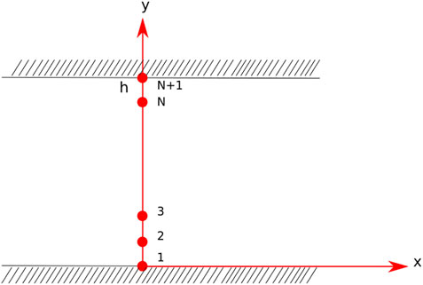
FIGURE 1. 1D channel flow with N + 1 grid points.
Finite difference methods are one of the standard numerical methods for solving PDEs. In this work, we use the second-order central difference scheme for space variables to discretize the PDE (2.1) over the channel width. Backward/Implicit Euler scheme is used for the time evolution of the channel flow.
The channel is divided into N intervals over 0 ≤ y ≤ h with N + 1 grid points. u(xi, t) represents the solution at the i the grid point at time t and is shortened to ui(t). Substituting the approximated operators in Eqs 2.1, 2.2 leads to:
Combining the equations for all the grid points, we obtain a system of linear equations:
where A and b have the following forms with
Solving 2.4 provides an approximate solution profile at time t + Δt.
3 Solving Channel Flow on DWAVE Quantum Annealer
In this section we describe our methodology to convert a fluid flow problem to a form amenable for the DWave machine. An adiabatic quantum annealer can solve problems posed as unconstrained binary optimization problem. This essentially means converting the system of equations in real variables into an optimization problem with binary variables.
Our approach uses two steps to convert the problem to QUBO. We first convert real variables to binary variables by using a fixed-point approximation. In the second step, we use a linear least-squares formulation to transform the problem to an optimization problem with binary variables. The following subsections discuss these two steps along with pre- and post-processing steps required by the annealer.
3.1 Quadratic Unconstrained Binary Optimization Formulation
In computing, fixed-point representation is one of the discrete representations for a real data type that has a fixed number of digits after a radix/fixed point. Essentially, it represents a real value by scaling an integer value with an implicit scaling factor which remains fixed throughout the computation. In (O'Malley and Vesselinov, 2016; Rogers and Singleton, 2019), this idea was used to convert real variables to binary variables by using a scaling factor of 2. Thus, the solution at the ith grid point, ui can be represented as
Here n is the precision of the representation, j0 is the position of the fixed point, and qj is the jth binary variable. Clearly, keeping the precision fixed while varying j0 leads to representing different ranges of the decimal values. Table 1 shows the range of real values for various precisions with fixed point after position 1 (the leftmost position is the starting bit). While increasing the precision(n) by one increases the range by an amount 1/2n+1, moving the fixed point position by one would lead to doubling the maximum value. Using 3.1 to represent the solution at each grid point by using n binary variables and substituting it in 2.4 leads to an extended matrix Ad such that Au = Adq. Finally, the linear system 2.4 becomes
Note that the right hand side of the linear system is unaffected by this transformation, and is a real data type.

TABLE 1. Maximum bound for reals for various precisions with fixed point after position 1.
Posing 3.2 in a least-squares form leads to the following optimization problem:
where Ad is a real-valued matrix, b is a real-valued vector and q is a binary vector.
As mentioned before, the annealer takes the QUBO form as an input:
Here vi and wij correspond to the weights associated with each logical qubit and the coupling strengths between two logical qubits of the problem that defines its energy landscape.
In order to convert 3.3 to the QUBO form, we expand the square and use the idempotent property of binary variables to obtain
3.2 Pre- and Post Processing
By design, the DWave annealer is organized as a lattice of unit blocks of qubits, where each block has eight qubits configured as a four-node bipartite graph. This hardware configuration is called a Chimera graph and is shown in Figure 2. As a result of this design, no three qubits are mutually coupled. This restricts the structure of the problem that the annealer can solve, and in general the logical problem needs to mapped or embedded to the hardware layout in a way that allows mutually coupled logical qubits.
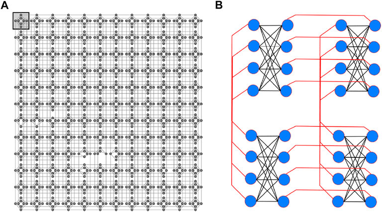
FIGURE 2. (A) DWave Hardware Chimera Graph, showing the layout of the physical qubits in DWave annealer. Each block in the Chimera graph is K4 graph. (B) Schematic of a unit block showing a schematic of a four block configuration where the blue represents a qubit with the coupling between adjacent blocks shown in red.
One way that DWave supports embedding generic layouts to its Chimera layout is by using the concept of chaining. Chaining allows linking or representing a single logical qubit with a chain of hardware qubits. This involves finding sub-graphs in the Chimera layout to embed the logical problem. Such a process increases the number of qubits required for the logical problem, and as a result restricts the size of the logical problem that can be solved as we will see in the results section.
In this work, we do not focus on the problem of obtaining optimal embeddings for our channel flow problem, and instead use the utilities provided by the SAPI libraries from DWave. The Solver API (SAPI) is an interface to the DWave QPUs along with a variety of other advanced software solvers. The client applications can use this API to develop their applications in C, MATLAB, and Python. The native embedding utility provides a mapping between the logical qubits to chained hardware qubits where the algorithm tries to embed larger strongly connected components first, then smaller components.
Algorithm (Figure 3) provides an overview of all the steps for solving the one-dimensional channel flow on the DWave annealer. For each time step, we use the QUBO solution obtained from the previous step to construct the right-hand-side input to the linear system. After each QUBO solve, all the states returned by the annealer are collected along with the number of occurrences of each state. Since, QUBO returns all possible solution states achieved by the hardware, we employ various strategies to compute possible solutions from the entire spectrum of returned solutions. Once a particular strategy is chosen, we transform the binary solution to a real type by using the transformation 3.1.
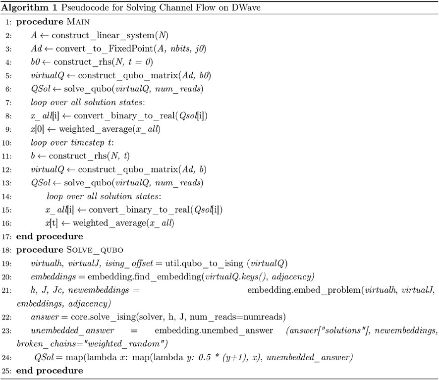
FIGURE 3. Pseudocode for solving channel flow on DWave.
In the next section, we report the results for the three key solution strategies (lowest energy, mean and weighted mean) that we use to study the effect of precision of the fixed-point representation when compared to the standard double-precision floating point arithmetic solutions for the channel flow.
4 Numerical Experiments
The flow parameters of the problem are shown in Table 2. We have used the DWave DW2X_3 hardware solver for obtaining the QUBO solutions for each time step of the flow. The number of grid points in the mesh was varied from 5 to 10 points including the boundary points, and the simulation was performed for 10 time steps. Specifically, the QUBO solution from the previous time-step was used to form the right hand side (rhs) of the new linear system. Table 3 shows the size of the logical QUBO with respect to the highest precision within the range 1–8 for which atleast one embedding was found by the DWave SAPI embedding utilities. For code development, a LANL Institutional Computing testbed, Darwin was used along with DWave SAPI utilities (sapi-c/3.0, sapi-python/3.0, sapi-matlab/3.0, qop/2.5.0.1, etc.). In the subsequent sections, we provide both qualitative and quantitative analysis of the solutions obtain from the hardware. In particular, we explore the following three key solution selection schemes:
• Lowest energy, i.e., the real-valued solution corresponding to the lowest energy state returned by the hardware,
• Unweighted mean, the mean of all real-valued solutions of all the states returned by the hardware, and
• Weighted mean, the mean of all real-valued solutions of all the states returned by the hardware weighted by their number of occurrences.
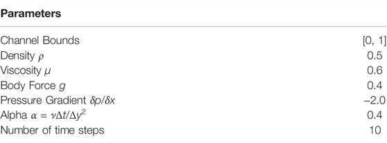
TABLE 2. Flow parameters used for the channel flow.
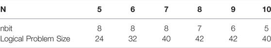
TABLE 3. Size of the logical problem with increasing number of grid points N (here N includes the boundary points) and precision n.
4.1 Effect of Precision
Figure 4 shows the profiles of the lowest energy solutions obtained from DW2X_3 solver for precision 2, 4 and 8. The results are shown for each of these three precisions for different grid resolutions - 5, 7 and 9 respectively. The last row shows the solution obtained using double-precision floating point arithmetic. For a mesh with nine grid points, the logical problem solution size for precision 8 is 56 bits for which no embedding was found by the SAPI embedding utility. Figure 5 shows the results for the same combinations (precisions 2, 4, 8 and number of grid points 5, 7 and 9 as well as the classical solutions using double-precision floating point arithmetic) but using an unweighted mean scheme, which means that the solution distributions obtained by SAPI are simply averaged, without any regard to their distributions (the number of times each solution vector is obtained and returned by SAPI). Figure 6 shows the results for the same combination in Figures 4, 5, but now using a weighted mean of the solution vectors, weighted by the number of times they are returned by SAPI for each draw. The purpose of showing all three schemes in Figures 4–6 is to highlight the fact that no standardized techniques are available in the literature which prescribes how to extract meaningful solutions from the annealer for problems of this nature as well as to study the sensitivity of the solutions to each of the three schemes described. For this purpose, all results are compared to the classical solution for the corresponding number of grid points. Also note that only nine iterations of the solution process are shown for each solution to maintain clarity in presentation and also due to limitations of resources in terms of allocation time on the machine and resources available for data analysis and postprocessing. However, this exercise is still useful to highlight the broad sensitivities of the solution space. We highlight several observations from Figure 4 below.
• The lowest energy solution state returned by the solver for lower precision’s are highly inaccurate. For precision 2, the solution yields a straight line, which is unrealistic.
• Unlike the classical solutions, which shows a systematic monotonic progression over each time step, the least energy solutions show a much more chaotic oscillatory behavior with no systematic progression over iterations steps.
• Only the solution with precision 8 resembles the shape of the classical profile qualitatively, although very crudely.
• Quantitatively, the peak values of the profile (expected to be parabolic from the classical solution) are higher by an order of magnitude. More details on the quantitative comparisons are provided in section 5.3.
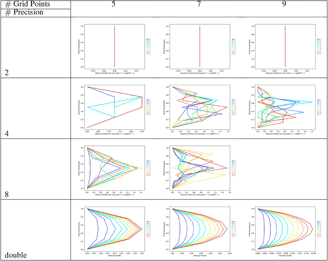
FIGURE 4. Solution profiles corresponding to the state with the lowest energy returned by the hardware for precision’s 2, 4, 8 and double for mesh with sizes 5, 7 and 9.
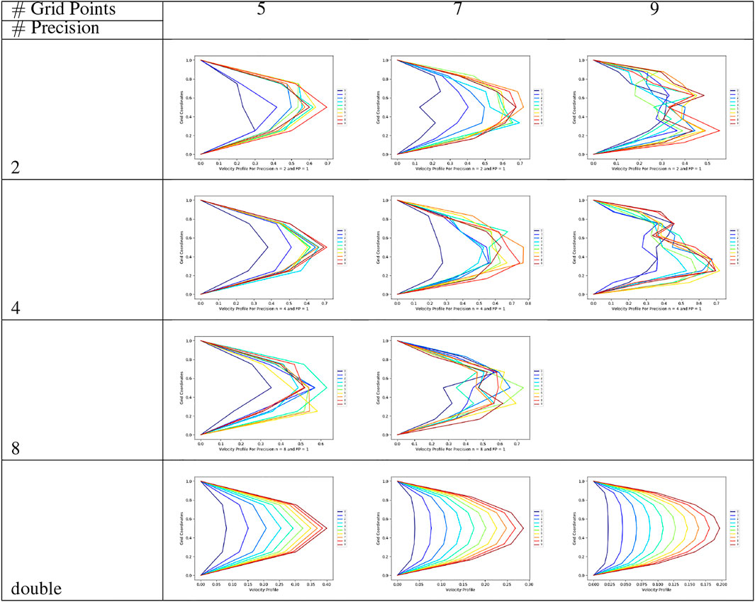
FIGURE 5. Solution profiles corresponding to unweighted mean state for precision’s 2, 4, 8 and double for mesh with sizes 5, 7 and 9.
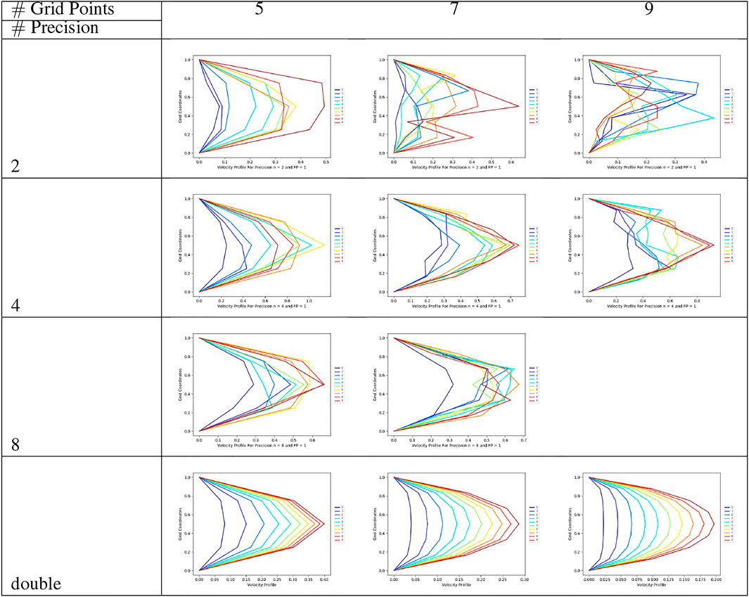
FIGURE 6. Solution profiles corresponding to weighted mean state for precision’s 2, 4, 8 and double for mesh with sizes 5, 7 and 9.
While the lowest energy solutions seem to be provide very crude approximations, the schemes with weighted and unweighted means perform better in comparison. We summarize the key observations from Figure 5 next.
• Most of the solutions show a systematic progress of the solution with the successive iterations.
• For all precision values, lower number of grid points (5 and 7) qualitatively capture the parabolic solution profile, although solution profiles start to degrade with the increase of precision and number of grid points.
• With nine grid points, the shape of the profile appears bimodal and is unrealistic.
• The peak value of the profile still deviates from the classical solution, however, the overall solution quality is better than the least energy formulation, in terms of error magnitude.
Hence it appears that using all the states than a single state based on the least energy can improve the quality of solution, but it is also dependent on the precision and grid size. To understand the sensitivity of the solutions when all states are used and weighted by their number of occurrences to obtain the mean is studied next. The following key observations are derived from Figure 6.
• Solutions do progress more systematically like the unweighted scheme, at least for five and seven grid points.
• For five grid points, solutions are quite close to the classical solutions across the iterations, and the solution quality improves with precision.
• For higher number of grid points, the solutions seem to improve with higher precision, which is an opposite behavior compared to the unweighted cases.
• The errors appear to be reduced with increase in precision and number of grid points.
4.2 Solution Distribution at Domain Center
To explain the difference in behavior between the schemes using unweighted and weighted means, the actual distributions of solutions at the domain center are plotted in Figure 7. It shows the aforementioned distributions (actual numbers of occurrences) for precision values of 2, 4, 6 and 8, each for 5, 7 and 9 grid points. For clarity of presentation, only 4 different iteration steps are plotted (1,4, 7 and 10). The key observations from Figure 7 are:
• For lower precision values, the number of occurrences of the state which corresponds to the real value zero occurs the highest number of times. With increase in the number of iterations and the number of grid points, non zero solutions start to appear a finite number of times. Thus, taking a simple unweighted mean will counter the effects of high frequencies of zero solutions. However, taking a weighted mean will push the final solution towards zero. This explains why taking an unweighted mean yields a better solution at lower precision values.
• At higher precision values, the non zero solutions start having more frequencies as expected. As the precision is increased further, the distributions also progressed finitely in time. As noticed in the figure, the time iterations of the distributions can be identified as separate clusters.
• At higher precision, taking a weighted mean seems to be a better strategy as that approach will represent the finite frequencies of non zero solutions across the solution space.
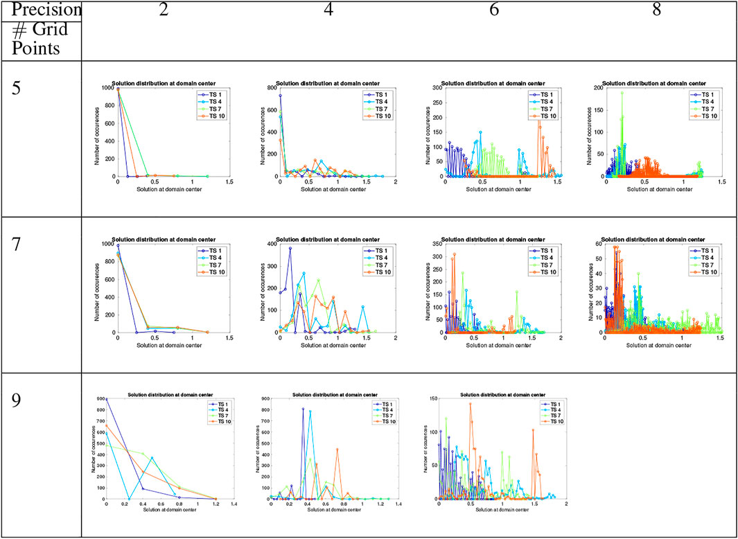
FIGURE 7. Solution distribution at domain center.
4.3 Error Analysis
Figures 8–10 summarizes the solutions by plotting the L2 and L∞ errors for 5, 7 and 9 grid points, respectively. Each of these figures show both types of errors for the unweighted and weighted schemes. The L2 error computes the Euclidean norm of the difference between the quantum solution and that of the classical solution. The L∞ error effectively computes the difference between the maximum value of the solution vector for the classical and the quantum solutions. Hence the L2 error represents the error for the entire solution space, and the L∞ error represents the error for the solution maximum, which represents the highest velocity within the domain, i.e., the center point of the domain. The errors are shown for all precision values (2–8) in Figures 8–10. We summarize the key observations from these figures below:
• For five grid points, the difference among different precision values are much lower for the unweighted scheme compared to the weighted scheme for both L2 and L∞ errors.
• For five grid points, both the L2 and L∞ errors are lower for higher precision values for unweighted solutions. Moreover, the errors seem to decrease with iterations, indicating potential convergence. The weighted mean solutions do not exhibit any clear pattern like this.
• For seven and nine grid points, the divergence among the weighted solutions seem to be larger compared to the unweighted scheme. However, errors seem to increase with higher precision and the lowest precision value seems to show the lowest L2 and L∞ errors. No clear pattern of convergence is found either.
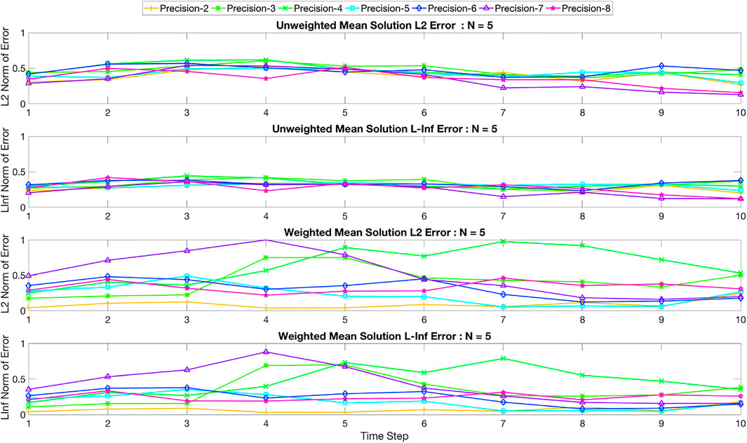
FIGURE 8. L2 and L∞ errors of the unweighted and weighted mean solutions for a problem with five grid points. The precision varies from 2 to 8 and the error is computed for each time step.
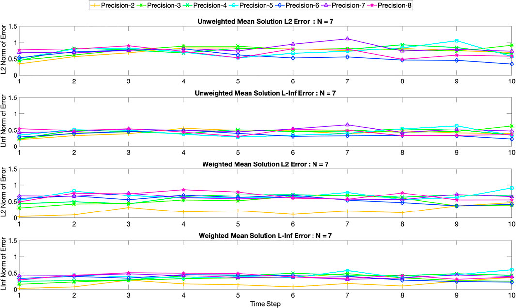
FIGURE 9. L2 and L∞ errors of the unweighted and weighted mean solutions for a problem with seven grid points. The precision varies from 2 to 8 and the error is computed for each time step.
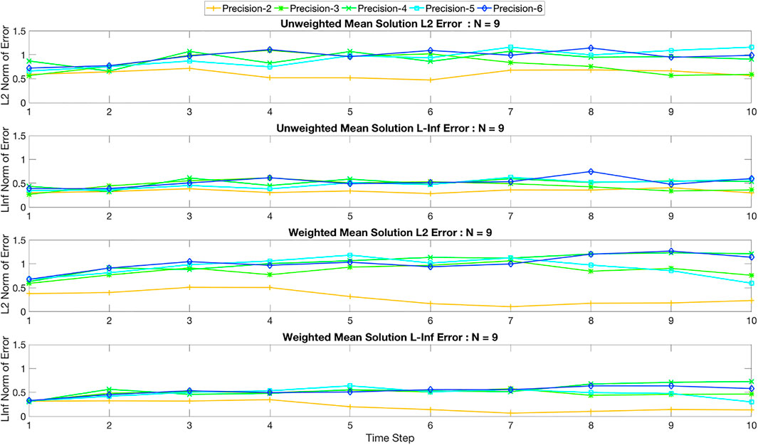
FIGURE 10. L2 and L∞ errors of the unweighted and weighted mean solutions for a problem with nine grid points. The precision varies from 2 to 8 and the error is computed for each time step.
5 Conclusion
In this work, we have demonstrated the potential, shortcomings and sensitivities of solving linear systems obtained from a reduced version of the Navier Stokes (NS) equation on the DWave quantum computer. We have chosen a very simple application, namely the one dimensional channel flow problem, where the classical solution is a well established parabolic flow. Using this reference solution we have explored how the system of linear equations obtained from the discretized form of the NS equations can be converted to a form amenable to the DWave Quantum annealer. This conversion involves a fixed point arithmetic based conversion of decimal to binary variables and posing the system in a least square formulation. This allows the construction of a quadratic unconstrained binary optimization (QUBO) problem, that is solvable by the DWave utilities. However, in this work, we have only used the default embedding of the DWave annealer (called a Chimera graph) which is organized as a lattice of unit blocks of qubits, where each block has eight qubits configured as a four-node bipartite graph. A technique called chaining allows one to use more optimized embeddings specific to the problem, and this is beyond the scope of the current work. In this work we have instead focused on the following questions:
• How to get extract the “correct” solution from the distribution of binary solution vectors?
• How do the different strategies for obtaining this solution compare to each other?
• What are the sensitivities of the obtained solutions to the grid resolution and precision value used in the fixed point arithmetic?
To answer these question we have plotted solution distributions at the domain center, compared three different methods (least energy, simple unweighted means and weighed means, where the weights are number of occurrences of each solution) to extract the quantum solutions against the classical solution, and performed error analysis to demonstrate the sensitivities with precision values and grid resolutions. We can answer the aforementioned questions as follows:
• There is no unique method to extract the correct solution.
• The least energy solution is the poorest. The weighted and unweighted means that involve all obtained solutions in each iterations provide better solutions consistently.
• At lower precision values, the unweighted means perform better. At higher precision values weighting the solutions with their numbers of occurrences is a better approach. Interestingly, increase of grid resolution and higher precision does not automatically allow more accurate solutions because it increases the noise of the system significantly. The unweighted mean solution doesn’t prefer any particular solution, which is why for lower precisions it has an effect of smoothing the solutions. On the other hand, as the weighted means captures the average of results weighted by their number of occurences, with good solution states with high number of occurences it would give a better approximation to the true solution. We see some effect of this, say for grid 5, precision 4 and 8, however, with increasing grid size we loose this behavior due to noisy results. Statistically in the scenario where the true solution states are returned by the QPU, we would observe that average solution (weighted and unweighted) converges with increasing sample space.
Overall, we observe that the solutions do not improve with increase in precision or grid size. Our intuition is that there are couple of limitations that affect solution accuracy. First, the values of the coefficients in the QUBO form are not represented at the same level of precision as described by the logical problem on the actual hardware due to the limitations on the ranges of the values for the physical parameters that the hardware can work with. Second, how the logical problem is being mapped to the hardware has an effect on the solution. In this work we have not focused on finding the best/optimal mapping of our logical problem graph to the hardware qubit graph. As we increase the precision, or grid size, the logical problem size increases. As a result, the mappings, which are obtained by using the utilities provided by the SAPI libraries, can (and do) use longer-chains of hardware qubits to represent a logical qubit, with more number of such longer chains present in the problem. Such a mapping is only “a” solution of the mapping problem, and may not be the best/optimal mapping solution for the logical problem. This whole process increases the total number of hardware qubits, which also contributes to noisy results.
To the best of our knowledge of the literature, this work is one of the first which demonstrates a simple workflow to reduce the Navier Stokes equations in a form readily solvable by the DWave machine (or quantum computers of the annealer type). This workflow can be followed to solve several problems spanning multiple disciplines ranging from solid to fluid mechanics and engineering, essentially any problem that can be reduced to linear systems of equations. The sensitivity of the workflow to the multiple parameters of the QUBO type solution process is perhaps of more interest than the accuracy of the solution instead. In future works, we will further explore the effects of more optimized embedding schemes. Moreover, the inherent nature of the DWave machine, which provides a large number of distributions at every step of the solution instead of one unique solution might allow one to explore Monte Carlo type approaches to solving linear systems of practical interest.
In this work, we have not addressed the problem of non-linearity that is part of any realistic fluid flow problem. Because, a fundamental limitation is imposed by the current QPU, which requires the logical problem to be in a QUBO form, including non-linear forms becomes non-trivial. As in standard discretization methods, we would have to approximate the non-linear forms to be a QUBO amenable approximation, which would include higher-order terms or non-linear forms. For high-order polynomial terms, there are methods that reduce the high-order form to a QUBO form via anciliary qubits (for example, (Perdomo-Ortiz et al., 2012)) along with extra constraints into the logical problem, which would significantly increase the logical problem size, and result in more noisy results. Such explorations into approximations of non-linear forms would be part of future studies.
Data Availability Statement
The raw data supporting the conclusions of this article will be made available by the authors, without undue reservation.
Author Contributions
NR, TB, BN, and SK all contributed to conception and design of the work. NR and TB implemented the suite of experiments and subsequent testing on the DWave hardware. All authors contributed to writing drafts and revision.
Funding
This work was supported under the ISTI Rapid Response Research Call for “Hands-on Quantum Computing 2018” at Los Alamos National Laboratory. Assigned: LA-UR-21-29172. Los Alamos National Laboratory is operated by Triad National Security, LLC for the National Nuclear Security Administration of U.S. Department of Energy under contract 89233218CNA000001. SK thanks the U.S. Department of Energy’s Biological and Environmental Research Program for support through the SciDAC4 program.
Conflict of Interest
The authors declare that the research was conducted in the absence of any commercial or financial relationships that could be construed as a potential conflict of interest.
Publisher’s Note
All claims expressed in this article are solely those of the authors and do not necessarily represent those of their affiliated organizations, or those of the publisher, the editors and the reviewers. Any product that may be evaluated in this article, or claim that may be made by its manufacturer, is not guaranteed or endorsed by the publisher.
Acknowledgments
The authors acknowledge the support from the Advanced Simulation and Computing Program (ASC), Los Alamos National Laboratory.
References
Chapuis, G., Djidjev, H., Hahn, G., and Rizk, G. (2019). Finding Maximum Cliques on the D-Wave Quantum Annealer. J. Sign Process Syst. 91, 363–377. doi:10.1007/s11265-018-1357-8
D-Wave Systems (2018). Dwave Software. Burnaby, Canada. Available at: https://www.dwavesys.com/.
Dahl, E. D. (2013). Programming with D-Wave: Map Coloring Problem. techre-port 604-630-1428. (Burnaby, BC: D-Wave Systems).
Gaitan, F. (2020). Finding Flows of a Navier-Stokes Fluid through Quantum Computing. npj Quantum Inf. 6, 61. doi:10.1038/s41534-020-00291-0
Neukart, F., Compostella, G., Seidel, C., von Dollen, D., Yarkoni, S., and Parney, B. (2017). Traffic Flow Optimization Using a Quantum Annealer. Front. ICT 4, 29. doi:10.3389/fict.2017.00029
O'Malley, D., and Vesselinov, V. V. (2016). “Toq.jl: A High-Level Programming Language for D-Wave Machines Based on Julia,” in 2016 IEEE High Performance Extreme Computing Conference (HPEC), Waltham, MA, September 13–15, 2016, 1–7. doi:10.1109/HPEC.2016.7761616
Perdomo-Ortiz, A., Dickson, N., Drew-Brook, M., Rose, G., and Aspuru-Guzik, A. (2012). Finding Low-Energy Conformations of Lattice Protein Models by Quantum Annealing. Sci. Rep. 2, 571. doi:10.1038/srep00571
Rogers, M. L., and Singleton, R. L. (2019). Floating-Point Calculations on a Quantum Annealer: Division and Matrix Inversion. arXiv e-prints,1901.06526.
Srivastava, S., and Sundararaghavan, V. (2019). Box Algorithm for the Solution of Differential Equations on a Quantum Annealer. Phys. Rev. A 99, 052355. doi:10.1103/PhysRevA.99.052355
Steijl, R., and Barakos, G. N. (2018). Parallel Evaluation of Quantum Algorithms for Computational Fluid Dynamics. Comput. Fluids 173, 22–28. doi:10.1016/j.compfluid.2018.03.080
Steijl, R. (2019). “Quantum Algorithms for Fluid Simulations,” in Advances in Quantum Communication and Information (London, UK: IntechOpen). chap. 3. doi:10.5772/intechopen.86685
Ushijima-Mwesigwa, H., Negre, C. F. A., and Mniszewski, S. M. (2017). “Graph Partitioning Using Quantum Annealing on the D-Wave System,” in Proceedings of the Second International Workshop on Post Moores Era Supercomputing, Denver, CO, November 12–17, 2017 (New York, NY, USA: ACM), 22–29. PMES’17. doi:10.1145/3149526.3149531
Keywords: quantum, adiabatic computing, fluid flow, Navier-Stokes, annealer
Citation: Ray N, Banerjee T, Nadiga B and Karra S (2022) On the Viability of Quantum Annealers to Solve Fluid Flows. Front. Mech. Eng 8:906696. doi: 10.3389/fmech.2022.906696
Received: 28 March 2022; Accepted: 08 June 2022;
Published: 04 July 2022.
Edited by:
Romit Maulik, Argonne National Laboratory (DOE), United StatesReviewed by:
Giuseppe Florio, Politecnico di Bari, ItalyPrakash Vedula, University of Oklahoma, United States
Copyright © 2022 Ray, Banerjee, Nadiga and Karra. This is an open-access article distributed under the terms of the Creative Commons Attribution License (CC BY). The use, distribution or reproduction in other forums is permitted, provided the original author(s) and the copyright owner(s) are credited and that the original publication in this journal is cited, in accordance with accepted academic practice. No use, distribution or reproduction is permitted which does not comply with these terms.
*Correspondence: Navamita Ray, bnJheUBsYW5sLmdvdg==
†Present address: Tirtha Banerjee, Department of Civil and Environmental Engineering, University of California, Irvine, Irvine, CA, United States