Review and perspectives in quantum computing for partial differential equations in structural mechanics

1 Introduction

Structural mechanics is often modeled by means of partial differential equations (PDEs). However, it is only for a small set of simple problems, domains and boundary condition that an analytical solution is known. In all other cases, engineers must rely on numerical techniques to obtain an approximate solution.

Given the importance of PDEs, research on convergence and accuracy of numerical solvers has dominated in the past decades. Nevertheless, the computational demand is still high whenever the domain is large with respect to the physics’ scale or when nonlinearities require a high level of detail of the numerical solution.

Potentially, quantum computing can revolutionize the field of numerical computational mechanics, thanks to its promise of unprecedented theoretical speed-up. For instance, the Harrow, Hassidim, Lloyd (HHL) algorithm (Harrow et al., 2009) can solve sparse linear systems exponentially faster than any classical method. At a first glance, it may seem that HHL could be applied to the discretized Poisson equation and exponentially reduce the runtime to obtain the displacement field of a loaded structure.

As tantalizing as they sound, almost all promises of quantum advantage are currently bound to theory and simulations and likely will be for the next few decades. What has yet to catch up with the algorithms is the hardware, which is still far from the technological requirements for practical quantum advantage.

This limitation gave reason to a separate branch of research, which abandoned the idea of proving quantum speed-up, but focused on algorithms that take into account the limitations of current hardware. These are mostly hybrid methods, that use a classical computer in combination with a quantum one, assigned to solve classically hard tasks. As with the theoretical speed-up algorithms, these hybrid methods also found application in the field of numerical PDE solving.

Given the importance and richness of the field, this review wants to be the first work to present and compare different quantum PDE solvers. Specifically, this work is aimed at the applied mechanics community and thus limits its focus to equations in structural mechanics. However, it must be pointed out that the field of quantum algorithms for PDEs spans many other branches of science, such as fluid mechanics (Mezzacapo et al., 2015; Steijl and Barakos, 2018; Todorova and Steijl, 2020; Gaitan, 2020, 2021; Budinski, 2021a,b), finance (An et al., 2020; Chakrabarti et al., 2021; Fontanela et al., 2021), model discovery (Heim et al., 2021) and cosmology (Mocz and Szasz, 2021), which may also benefit from specialized reviews.

This paper is structured as follows. Section 2 presents some standard concepts of quantum computing and explains the quantum algorithms at the root of PDE-solving. Section 3 reviews the literature on quantum algorithms for linear PDEs, while Section 4 is devoted to nonlinear PDEs. Finally, Section 5 provides concluding remarks and discusses possible future prospects of quantum computation applied to structural problems.

2 Main concepts of quantum PDE solving

At the time of writing, almost no quantum algorithm applies to all possible combinations of partial differential equations, boundary conditions, discretizations, etc. However, one can trace out a generic PDE-solving workflow, as in Figure 1. Here it is important to notice that quantum computation takes place only in the so-called quantum primitive, i.e. an algorithm that acts on quantum states by means of quantum operators. Also, the quantum primitive does not alone solve the PDE, but rather its discrete form, which generally is the computational bottleneck in classical logic.

FIGURE 1

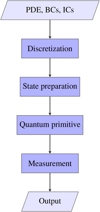
FIGURE 1. Workflow of the process of solving partial differential equations with a quantum primitive. The input is given, in the general case, by the PDE together with its boundary (BCs) and initial (ICs) conditions. After the differential problem has been discretized with schemes such as finite elements or finite differences, the input data is encoded into a quantum state (state preparation step). The quantum primitive then produces the solution to the discrete problem as a quantum state. However, the information in this state cannot be accessed, as this is generally in quantum superposition. Therefore, quantum PDE solver also needs to measure the state after the quantum primitives as many times as required by the user-defined solution precision. Depending of the application, such measurement are postprocessed to provide the final output.

Furthermore, in contrast to a classical algorithm, a quantum primitive does not operate in the same environment in which the data is stored and read-out. In other words, there is a state-preparation step prior to quantum computation, where classical data is encoded as a quantum state, as well as a measurement step afterwards, that provides output in classical form.

A similar workflow was previously proposed (Pesah, 2020), where the author points out that a discretized PDE can be mapped either to a Schrödinger equation or to one or more linear system(s). In the first case, one may use Hamiltonian simulation to obtain the solution in quantum state, while linear systems could be solved by the HHL algorithm or more efficient quantum linear solvers. However, this classification concerns only linear PDEs and does not consider algorithms that are not fully quantum (i.e. all computations from quantum-form data to quantum-form solution are done on a quantum computer) or quantum annealing.

This section gives the necessary background on the ‘quantum-block’ of PDE solving, that concerns the last three steps in Figure 1.

2.1 Quantum state preparation

The problem of quantum state preparation arises every time classical data needs to be encoded as a quantum state and it is by no means restricted to quantum PDE solvers. Taking the homogeneous heat equation as an example, one needs to encode an initial condition u₀(x) in a quantum register. First, space-discretization transforms u₀(x) into the discrete array of gridpoint values u₀ of N entries. Then, this vector is normalized to turn it into the suitable quantum state

$\left|u_0\right.⟩=\frac{{\mathbf{u}}_0}{{‖{\mathbf{u}}_0‖}_2}.(1)$

The vector on the left hand side of Eq. 1 is called ket vector, according to the so-called braket notation (Nielsen and Chuang, 2010).

Furthermore, $\left|u_0\right.⟩$ can be written as a vector of N complex amplitudes defined with respect to a chosen basis, i.e.

$\left|u_0\right.⟩=\sum _{j=0}^{N-1}{u}_{0,j}\left|b_j\right.⟩,$

where $u_{0,j}\in \mathbb{C}$ are the amplitudes and $\left|b_j\right.⟩$ are the basis states. Since many quantum computer models work with binary physical systems (qubits), the basis $\left\{\left|b_j\right.⟩\right\}$ is defined as the set of all possible states of $n=\lceil {\log }_2\left(N\right)$ such systems (log₂ will be subsituted by log in the following, for simplicity of notation). By labelling the states of a qubit as 0 and 1, the basis states are written as

$\left|00\dots 00\right.⟩,\left|00\dots 01\right.⟩,\left|00\dots 10\right.⟩,\dots ,\left|11\dots 11\right.⟩,$

which constitute the so-called computational basis. It is easy to see that the computational basis forms an orthonormal basis, since, given two basis vectors b_i and b_j

$⟨b_i|b_j⟩={\delta }_{ij},i,j\in \left\{\mathrm{1,2},\dots N\right\},$

where δ_ij is the Dirac delta.

One should keep in mind that the computational basis is just one of the infinite possible bases in the ${\mathbb{C}}^N$ space and that any other binary orthonormal set of vectors form an equally valid basis for the same space.

Furthermore, the braket notation implies a unit norm vector, that is

$\sum _{j=0}^{N-1}{u}_{0,j}^2=1.(2)$

Equivalently, Eq. 2 states that the squared amplitudes of a ket vector can be seen as probability amplitudes, modelling the fact that a n-qubits system will collapse to the basis state $\left|b_m\right.⟩$ with probability $u_{0,m}^2$ upon measurement.

Having access to the amplitues, the problem of state preparation becomes to evolve an initial state up to the state $\left|u_0\right.⟩$. This can be expressed in formulas,

$\left|u_0\right.⟩=U{\left|0\right.⟩}^{\otimes n},$

where U is a unitary operator representing the quantum state evolution and ${\left|0\right.⟩}^{\otimes n}$ is a conventional initial state where all qubits are in state $\left|n\right.⟩$. From now on, the initial state ${\left|0\right.⟩}^{\otimes n}$ will mostly be represented simply as $\left|0\right.⟩$, except when the number of qubits is not immediately evident from the context.

Clearly, the cost of implementing U influences the overall cost of solving the differential problem. In fact, preparing a generic quantum state over n qubits requires O(N) quantum gates (Nielsen and Chuang, 2010), where the “big O” notation represents the asymptotic upper bound on the number of computational resources. Therefore, even if the quantum primitive runs in $O\left(\log \left(N\right)\right)$ time, the task of numerically evolving the initial condition on a quantum comptuer might still take $O\left(N\right)$ time overall. Fortunately, several probability distributions can be prepared efficiently (i.e. in logarithmic time). Interesting instances for numerical analysis are polynomials defined over a regular grid or locally-supported functions in the case of the finite element method (FEM) (Montanaro and Pallister, 2016).

2.2 Hamiltonian simulation

One of the motivations that drove to the study of quantum computers was to simulate quantum systems, that are hard to simulate classically. Generally speaking, one aims at describing the evolution of a quantum state $\left|\psi \right.⟩$, which is described by the Schrödinger equation

$\frac{\mathrm{d}}{\mathrm{d}t}\left|\psi \right.⟩=-iH\left|\psi \right.⟩,(3)$

where H is the system’s Hamiltionian, i.e. a Hermitian matrix. For the sake of explanation, the Hamiltonian is considered here as time-invariant.

Hamiltonian simulation consists in evolving an initial quantum state $\left|{\psi }_0\right.⟩$ according to Eq. 3 on a quantum computer. Interestingly for this discussion, some partial differential equations can be rewritten as Schrödinger equations after a semi-discretization in space (Costa et al., 2019; Pesah, 2020; Suau et al., 2021). For this reason, quantum algorithms for Hamiltonian simulation can be used as quantum primitives to solve PDEs.

Eq. 3 has the exact solution

$\left|\psi \right.⟩=e^{-iHt}\left|{\psi }_0\right.⟩,(4)$

where e^−iHt is a unitary operator, due to the fact that H is Hermitian. Therefore, e^−iHt is a valid quantum operation that could be applied to $\left|{\psi }_0\right.⟩$. However, the exponential of a arbitrary Hamiltonian does not correspond, in general, to any known quantum circuit. In other words, the Hamiltonian H is difficult to simulate directly.

However, one can see H as a sum of Hermitian matrices that are efficient to simulate. In that case

$H=\sum _i{c}_i{H}_i(5)$

and $\left|\psi \right.⟩=e^{-i{\sum }_i{c}_i{H}_{i}t}\left|{\psi }_0\right.⟩$. The number of terms in Eq. 5 is what determines the complexity of Hamiltonian simulation. In fact, the generic Hamiltonian decomposes in a number of known evolution operators that is exponential in the dimension of the physical systems. Even though one may hope to re-write Eq. 5 as a product of exponentials, the H_i do not generally commute, i.e.

$\left[H_i,H_j\right]=H_i{H}_j-H_j{H}_i\ne 0$

for some i and j. Anyway, by dividing the evolution time in r subsequent time intervals Δt = t/r, the single H_i Hamiltonians can be evolved separately over Δt. This evolution over the sub-interval is then repeated r times. In the end, the overall operator is an approximation of the actual evolution of the total Hamiltonian H over t as stated, for instance, by the Trotter’s formula (Trotter, 1959):

$e^{-iHt}={\left(\prod _i{e}^{-i{c}_i{H}_{i}t/r}\right)}^r+O\left({\left(\mathrm{\Delta }t\right)}^2\right),(6)$

The importance of H and H_i being easy to simulate is clear from the Hamiltonian simulation runtime using product formulas. This is O(f(n)t/ɛ) (Nielsen and Chuang, 2010), where n is the number of qubits and ɛ is the desired Hamiltonian simulation error. While f(n) = poly(n) for simulatable Hamiltonians, f(n) = exp(n) in the general case, making for an exponential difference in the runtime.

In quantum physics, many natural systems are described by so-called local Hamiltonians, which are operators that act nontrivially on a few qubits and are known to be efficiently simulatable (Nielsen and Chuang, 2010). However and most importantly for PDEs, it was shown that also sparse Hamiltonians can be simulated in $O\left(\mathrm{p}\mathrm{o}\mathrm{l}\mathrm{y}(n)\right)$ time (Aharonov and Ta-Shma, 2003).

Finally, we remark that recent work exponentially reduced the dependency on precision (Berry et al., 2014; 2015a) and also achieved an optimal dependency on the sparsity (Berry et al., 2015a). Most recently, an approach based on qubitization achieved an additive lower bound with respect to t and 1/ɛ (Low and Chuang, 2019).

2.3 Quantum linear solvers

Linear systems arise in several numerical methods for PDEs and their solution often dominates the cost of the overall classical PDE algorithm. After appropriate discretization, the PDE assumes the familiar form Ax = b, which is a linear system in the N-dimensional space, N being the number of unknowns, which can correspond to the number of gridpoints, particles or harmonic basis functions, depending on the method of discretization used.

If the matrix A is positive definite, the fastest general-purpose classical linear system solver is the conjugate gradient method (Shewchuk, 1994). This algorithm has asymptotic time complexity

$O\left(Ns\sqrt{\kappa }\log \left(1/\epsilon \right)\right),(7)$

where s is the matrix sparsity, κ is the conditioning number and ɛ is the desired error for a certain precision metric.

What motivated the study of linear solvers beyond classical computation is the conjecture, due to complexity arguments, that classical algorithms cannot invert A in time $O\left(\log \left(N\right)\right)$ (Harrow et al., 2009). On the other hand, Harrow, Hassidim and Lloyd were the first ones to prove that a quantum algorithm based on the $O\left(\log \left(N\right)\right)$ sparse Hamiltonian simulation and phase estimation could solve linear systems exponentially faster in N (Harrow et al., 2009). In particular the time complexity of the HHL algorithm is

$O\left(s^2{\kappa }^2\log \left(N\right)/\epsilon \right).(8)$

However, the HHL algorithm and subsequent quantum linear solvers, do not solve Ax = b, but rather

$A\left|x\right.⟩=\left|b\right.⟩,(9)$

known as quantum linear system problem (QLSP). It is important to keep in mind that quantum linear systems algorithms (QLSAs) output the solution $\left|x\right.⟩=A^{-1}\left|b\right.⟩$ without accounting for preparation of $\left|b\right.⟩$ or measurement of $\left|x\right.⟩$, even though the cost of these operations could (and generally does) trump that of preparing $\left|x\right.⟩$.

The complexity of solving the QLSP was improved by later contributions. In terms of conditioning number, Ambainis et al. reduced the dependency from O(κ²) to O(κ) using variable time amplitude amplification (VTAA) for post-selecting the solution (Ambainis, 2012). Also concerning the conditioning number, Clader et al. showed how to include the use of a preconditioner in quantum linear solvers in order to deal with ill-conditioned matrices (Clader et al., 2013). Later on, an approach based on linear combination of unitaries was proposed to replace the phase estimation step, reducing the dependency on precision to $O\left(\mathrm{p}\mathrm{o}\mathrm{l}\mathrm{y}\log \left(1/\epsilon \right)\right)$ (Childs et al., 2017). Furthermore, an approach inspired by the adiabatic principle was also developed, achieving similar complexity compared to Ambainis’ work on VTAA (An and Lin, 2019; Subaşı et al., 2019).

Finally, several authors recently proposed to solve the QLSP with variational quantum algorithms (VQAs) (An and Lin, 2019; Bravo-Prieto et al., 2019; Huang et al., 2021; Xu et al., 2021; Patil et al., 2022), to be discussed later. These algorithms are appealing since they are suitable for implementation on near-term devices and require only shallow quantum circuits. However, VQAs are heuristics, meaning that the number of iterations needed for convergence depends on the choice of the optimization strategy. Thus, no theoretical runtime is known a-priori for VQAs. However, a recent study showed that VQA-based linear solvers include a quantum state verification step that requires at least $\mathrm{\Omega }\left({\kappa }^4\right)$¹ number of queries to the unitary preparing the state $\left|b\right.⟩$ (Somma and Subaşı, 2021).

2.4 Amplitude amplification and amplitude estimation

Amplitude amplification is an algorithm that iteratively promotes the probability of one or more amplitudes of a quantum state. This technique derives directly from Grover’s algorithm for database search (Grover, 1996, 1997). In this problem, a database and a function f are given. The database contains N = 2ⁿ entries, each of which is a n-bits string, such as

$x=x_0{x}_1\dots x_n,x_i\in \left\{\mathrm{0,1}\right\}.$

The function f marks the target bitstring m as follows

$f\left(x\right)=\left\{\begin{array}{cc}1\hfill & \text{if}x=m\hfill \\ 0\hfill & \text{otherwise}\hfill \end{array}\right..$

Classical search methods require to check the bitstring individually and therefore scale as O(N) and require N − 1 queries in the worst case. On the other hand, Grover’s algorithm works with all database entries in superposition and progressively promotes the amplitude of the target state $\left|m\right.⟩$. For instance, a good starting state is the unbiased uniform superposition

$\left|{\psi }_0\right.⟩=\frac{1}{\sqrt{N}}\sum _{j=0}^{N-1}\left|j\right.⟩,$

where each j represents one of the N bitstrings.

The quantum search algorithm consists in applying the Grover’s operator

$G=-\left(\mathbb{1}-2\left|{\psi }_0\right.⟩\left.⟨{\psi }_0\right|\right)\left(\mathbb{1}-2\left|m\right.⟩\left.⟨m\right|\right)(10)$

k times, where the outer product notation is used for $\left|{\psi }_0\right.⟩\left.⟨{\psi }_0\right|$ and $\left|m\right.⟩\left.⟨m\right|$, that are the projectors onto the initial and target states respectively ². It is easy to show that $k=O\left(\sqrt{N}\right)$ iterations are needed to prepare $\left|m\right.⟩$ with high probability. Therefore, the quantum search algorithm is quadratically faster than any classical one. This quadratic speed-up can be understood intuitively by thinking that each time Grover’s operator changes the amplitudes of the superposition, the probabilities change quadratically as much.

Even though G contains the target state $\left|m\right.⟩$ in its expression, it is not necessary to know it explicitly. In fact, the circuit of G uses an oracle for f, which is an operator such that

$O_f\left|x\right.⟩\left|0\right.⟩=\left\{\begin{array}{cc}\left|x\right.⟩\left|1\right.⟩\hfill & \mathrm{i}\mathrm{f}x=m\hfill \\ \left|x\right.⟩\left|0\right.⟩\hfill & \mathrm{o}\mathrm{t}\mathrm{h}\mathrm{e}\mathrm{r}\mathrm{w}\mathrm{i}\mathrm{s}\mathrm{e}\hfill \end{array}\right.,$

where the tensor product is implied between neighbouring ket vectors.

Therefore, the knowledge of $\left|m\right.⟩$ is included in the oracle O_f, which flips an ancilla qubit when the state register is in the target state. The specifics of the oracles depend on the different problems and go beyond the scope of this discussion, but suffices to say that they generally entail a unitary contolled by a n = ⌈ log  N⌉ register, such that the unitary gets applied only when such register is in state $\left|m\right.⟩$ (or is in a superposition with nonzero probability of measuring $\left|m\right.⟩$).

The concept of quantum search was extended to multiple target states with quantum amplitude amplification (QAA) (Brassard, et al. 2000). In this case, the Hilbert space spanned by the database is divided into a “good” subspace, containing the target states and a complementary “bad” subspace. Therefore, the Grover’s operator becomes

$G=-\left(\mathbb{1}-2\left|{\psi }_0\right.⟩\left.⟨{\psi }_0\right|\right)\left(\mathbb{1}-2P_g\right),(11)$

where P_g is the projector onto the “good” subspace. Also in this case a target state can be prepared quadratically faster than by using a classical search.

QAA is used as a subroutine in many quantum algorithms that require post-selection. This is usually a procedure used as the last step of a quantum computation, when a quantum register of interest contains the solution state with finite probability and it is entangled to an ancilla qubit in such a way that measuring the latter in one of its two states will collapse the register to the solution state. Therefore post-selecting requires to repeat the entire quantum routine until the correct measurement of the ancilla is obtained. For instance, in the case of many quantum linear solvers, the state before post-selection is

$\left|\text{trash}\right.⟩\left|0\right.⟩+\left|x\right.⟩\left|1\right.⟩,$

where $\left|x\right.⟩$ is the solution of the QLSP and $\left|\text{trash}\right.⟩$ represents the rest of the Hilbert space. In this case QAA amplifies the probabilities of the states that have the ancilla register equal to 1.

Quantum amplitude estimation (QAE) allows to compute the probability of one component of a quantum state. The main idea is to perform quantum phase estimation on Grover’s operator. In fact, the action of G on a state $\left|\psi \right.⟩$ is a rotation of an angle 2θ in the plane defined by the components of $\left|\psi \right.⟩$ in the “good” and “bad” subspaces (see Figure 2). In this 2-dimensional space,

$G=\left[\begin{array}{cc}\hfill \cos 2\theta \hfill & \hfill -\sin 2\theta \hfill \\ \hfill \sin 2\theta \hfill & \hfill \cos 2\theta \hfill \end{array}\right]=e^{iY2\theta },(12)$

where Y is the Pauli-Y operator, i.e.

$Y=\left[\begin{array}{cc}\hfill 0\hfill & \hfill -i\hfill \\ \hfill i\hfill & \hfill 0\hfill \end{array}\right].$

FIGURE 2

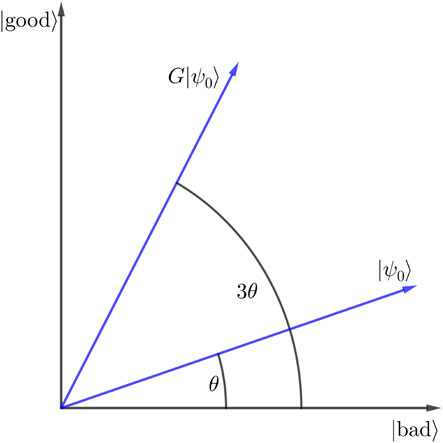
FIGURE 2. Effect of one Grover iteration used in quantum amplitude amplification. The axes represent the components of $\left|{\psi }_0\right.⟩$ in the “good” subspace and in the complementary “bad” subspace.

Therefore, quantum phase estimation on G returns an approximation of 2θ. In turn, this allows to compute the probability of the ‘good’ component of $\left|\psi \right.⟩$, since

${\left|{\psi }_g\right|}^2=⟨\mathrm{g}\mathrm{o}\mathrm{o}\mathrm{d}|\psi ⟩={\sin }^2\theta ,$

where $⟨\mathrm{g}\mathrm{o}\mathrm{o}\mathrm{d}|\psi ⟩$ is a notation used for inner products between vectors, but it is here extended to represent the projection of $\left|\psi \right.⟩$ onto the ‘good’ subspace.

Quantum amplitude estimation is useful, for instance, to estimate the integral of a PDE solution over a certain region S, i.e. ${\int }_{S}u\left(x\right)\mathrm{d}x$ (Linden et al., 2020). As it will be clear from the following section, scalar quantitites of this type are generally the output of quantum routines for PDEs.

2.5 Variational quantum algorithms

Variational quantum algorithms (VQAs) are the main class of methods conceived to run on current or near-future devices, better known as Noisy Intermediate Scale Quantum (NISQ) (Preskill, 2018). These early-stage quantum computers use up to a few hundreds of the so-called physical qubits, which are affected by noise of different nature, as opposed to logical qubits, that instead are made of many physical qubits that act as a fully error-corrected qubit.

Besides being suitable for near-term applications, VQAs are thought to be candidates for quantum advantage, in areas such as quantum chemistry, nuclear physics, but also optimization and machine learning (Cerezo et al., 2021a).

The small circuit depth is achieved via a hybrid strategy internal to an optimization process. At every iteration, a cost function is evaluated by the quantum computer and fed to the classical one, which updates the design parameters according to an optimization algorithm. Figure 3 schematically shows the working principle of VQAs.

FIGURE 3

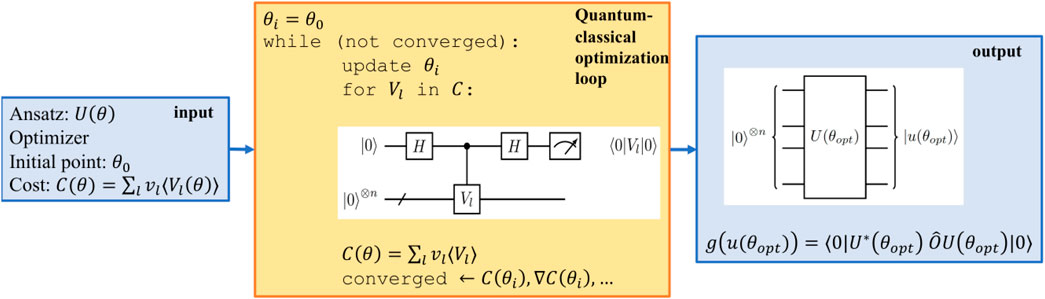
FIGURE 3. Working principle of variational quantum algorithms. The input are the hyperparameters, such as ansatz, optimizer and type of cost function and the initial value of the ansatz parameter. The cost is shown here as a linear combination of expectation values of unitaries, although other expressions are possible. In the quantum-classical optimization loop, the classical computer is in charge of updating the parameters θ according to the optimization logic, while the quantum computer evaluates the cost function terms. At the end of the optimization, the optimal parameter set θ_opt can be used to reconstruct the approximate solution as a wavefunction $(\left|u(\mathit{\theta })\right.⟩=U(\mathit{\theta }){\left|0\right.⟩}^{\otimes n})$ or in a larger circuit to obtain a scalar function of the solution g(u).

A comprehensive review of VQAs, their main concepts, applications and future prospects is given in (Cerezo et al., 2021a). In what follows, only a succint explanation is given about the main elements of these algorithms.

2.5.1 Ansatz

The ansatz is a parametrized unitary U(θ) that encodes the tentative solution to the problem, depending on the parameters θ. At the end of the optimization, the optimal parameters will define the solution’s approximation as U(θ_opt).

There exist many different families of ansatze, but a first important distinction is between the so-called problem-inspired ones, that incorporate information about the problem, and the problem-agnostic ones. For instance, a good example of the problem agnostic class is the so-called hardware-efficient ansatz (Kandala et al., 2017), which optimizes the use and distribution of gates according to hardware specification. On the other hand, examples of problem-inspired ansatze are the Unitary Coupled Clustered ansatz (Taube and Bartlett, 2006) and the Quantum Alternating Operator Ansatz (Farhi et al., 2014; Hadfield et al., 2019).

2.5.2 Cost function

The cost function C(θ) is a metric of how far the tentative solution at the current iteration is from the actual solution of the problem. In VQAs, the cost function is computed by measuring one or more observables of the ansatz state $U(\mathit{\theta })\left|0\right.⟩$. The type and number of observables are determined by the specific problem.

Some of the requirements for a good cost function apply to quantum as well as classical methods. For instance, the minimum of C(θ) must coincide with the solution of the problem and decreasing values of the cost function should correspond to better approximations of the solution. However, a good cost function for VQAs also needs to be hard to evaluate classically, since it would otherwise negate the possibility of quantum advantage (Cerezo et al., 2021a).

2.5.3 Gradient

Many optimization routines use the cost function gradient to identify the direction of maximum descent to speed-up convergence. Often however, the cost function does not have an analytical expression and the gradient needs to be computed using finite differences. Nevertheless, a quantum-evaluated cost function is noisy in its nature, due to finite sampling and hardware noise, so the finite difference approximation can be highly imprecise.

Luckily, the so-called parameter-shit rule (PSR) allows to compute gradients analytically using two cost function evaluations, similar to what happens in finite differences. The derivative of the cost C with respect to the lth parameter is then

$\frac{\partial C}{\partial {\theta }_l}=\frac{1}{2\sin \alpha }\left(C\left({\mathit{\theta }}^{+}\right)-C\left({\mathit{\theta }}^{-}\right)\right),(13)$

where θ^± = θ ± αe_l, e_l is the vector with 1 in the lth entry and 0 in all others and α is the magnitude of the shift.

Even though Eq. 13 looks similar to the finite difference formula, the two differ by the term $\frac{1}{2\sin \alpha }$. When the shift is α = π/2, the difference in statistical error between finite differences and PSR is maximum (Mari et al., 2021).

2.5.4 Optimizer

Optimizers for VQAs need to account for different complications that arise from a quantum-evaluated cost landscape. In fact, this is usually affected by stochastic and hardware noise or it can be flat with minima in narrow gorges, due to the phenomenon of barren plateaus (McClean et al., 2018; Cerezo et al., 2021b).

A main classification of VQA optimizers is between gradient-based and gradient-free algorithms. In principle, any classical optimizer can be used in VQAs, but the noisy character of the cost function makes some choices better suited than others to avoid stability and convergence issues. For instance, gradient-based techniques generally implement some form of stochastic gradient descent (SGD) methods, such as Adam (Kingma and Ba, 2015) or use natural gradients (Stokes et al., 2020). On the other hand, the simultaneous perturbation stochastic approximation (SPSA) method is probably the most popular gradient-free technique (Spall, 1992).

2.6 Quantum annealing

Quantum annealing (QA) is an algorithm that can solve combinatorial optimization (CO) problems. These require to search among a finite set of variables or choices with the aim is to find the “best” one according to a certain metric of merit. Importantly, many combinatorial optimization problems are NP-hard, meaning that finding their solution is difficult. More precisely, NP-hard problems are at least as difficult to solve as the most difficult problem in the NP complexity class, which includes all problems that can be verified in polynomial time by a nondeterministic algorithm. The NP class should be seen in contrast to the P class, which instead includes all problems that can be solved “efficiently”, i.e. in polynomial time using a deterministic algorithm. Given their hardness, CO problems are practially solved approximately, and the challenge is to produce accurate approximate solutions in short (polynomial) time.

However, QA cannot encode and solve a combinatorial optimization problem in generic form. Instead, the physical problem solved by QA is the one of finding the ground state of the Ising Hamiltonian (McGeoch, 2020).

$H_{\text{Ising}}=\sum _i^n{H}_i{q}_i+\sum _{\left(ij\right)}{J}_{ij}{q}_i{q}_j,(14)$

where q_i, q_j represent the binary values associated to the qubits, e.g. $\left\{\mathrm{0,1}\right\}$. These can indicate, for instance, the two different spins of a qubit. Also, $h_i\in \mathbb{R}$ is the local field at site i and $J_{ij}\in \mathbb{R}$ is the interaction strength between qubits i and j.

In order to reach to the ground state of H_Ising, the quantum annealing process starts from an initial Hamiltonian H₀, whose ground state is known and easy to prepare. A common choice for H₀ is the transverse magnetic field

$\sum _i^n-X_i,(15)$

X_i being the Pauli-X operator acting on the ith qubit, where

$X=\left[\begin{array}{cc}\hfill 0\hfill & \hfill 1\hfill \\ \hfill 1\hfill & \hfill 0\hfill \end{array}\right]$

From here, the system’s Hamiltonian is slowly changed according to an evolution law, such that

$H\left(t\right)=\left(1-f\left(t\right)\right)H_0+f\left(t\right)H_{\text{Ising}}\mathrm{f}\mathrm{o}\mathrm{r}t\in \left[0,T\right].(16)$

Here, T is the total evolution time, $f(t)\in \left[\mathrm{0,1}\right]$ and f(0) = 0, f(T) = 1. If H(t), known as the total Hamiltonian, is changed slowly enough, then the adiabatic principle ensures that the system’s configuration is at the ground state of H(t) at all times (Kato, 1950). At the end of adiabatic evolution, the system will therefore be in the ground state of the Ising Hamiltonian, which corresponds to the approximate solution of the CO problem.

However, quantum annealers operate with spin systems, where each spin s_i is a binary variable equal to ±1. Thus, QA programmers need to recast the CO problem to a binary optimization one. In D-Wave machines, which are the state-of-the-art quantum annealers, the problem is given as input in the Quadratic Unconstrained Binary Optimization (QUBO) form, that is

$\begin{array}{cc}\hfill \mathrm{m}\mathrm{i}\mathrm{n}\mathrm{i}\mathrm{m}\mathrm{i}\mathrm{z}\mathrm{e}& {\mathbf{q}}^{\top }Q\mathbf{q}\hfill \\ \hfill \mathrm{w}\mathrm{i}\mathrm{t}\mathrm{h}& \mathbf{q}\in {\left\{\mathrm{0,1}\right\}}^n,\hfill \end{array}(17)$

where $Q\in {\mathbb{R}}^{n\times n}$. The QUBO problem in Eq. 17 can be turned into the Ising Hamiltonian ground state problem by using the mapping s_i = 2q_i − 1.

2.7 Measurement

At the end of the quantum primitive the problem’s solution is encoded as a quantum state. This is a unit vector $\left|u\right.⟩\in {\mathbb{C}}^N$, but its information cannot be accessed without measurement. However, it is easy to realize that measuring the entire state vector would require O(N) measurements, breaking any speed-up obtainable with a quantum primitive.

Therefore, quantum computing becomes appealing for PDEs when the aim is to compute a certain scalar function g(u) of the solution. This function is often taken as the expectation value of an observable M, i.e.

$g\left(u\right)\propto ⟨M⟩:=\langle u|M|u\rangle .$

In principle, estimating ⟨M⟩ would require to measure $\left|u\right.⟩$ in the basis constituted by the eigenvalues of the operator M. However, this basis is not known in general and one needs to resort to methods other than direct measurement. One popular technique is the Hadamard Test (Aharonov et al., 2009), which assumes that M is a unitary operator. As showed in Figure 4, M is controlled on an ancilla qubit set in uniform superposition and later measured in the Pauli-X basis. It is easy to show that

$\mathrm{R}\mathrm{e}\left\{⟨M⟩\right\}=\frac{1}{2}\left(\mathrm{Pr}\left(0\right)-\mathrm{Pr}\left(1\right)\right),(18)$

where Pr(0) and Pr(1) are the probabilities of the ancilla qubit collapsing to $\left|0\right.⟩$ and $\left|1\right.⟩$ respectively.

FIGURE 4

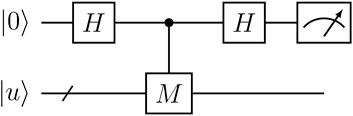
FIGURE 4. Hadamard Test circuit for computing ⟨u|M|u⟩. Oppositely to standard observable measurements, M needs to be unitary.

A recurrent case in applications is to estimate how “close” a state $\left|u\right.⟩$ is to reference state $\left|u_{\text{ref}}\right.⟩$. This can be accomplished using the SWAP Test (Buhrman et al., 2001), which is a Hadamard test where M is equal to the SWAP gate. If $\left|{\psi }_1\right.⟩$ and $\left|{\psi }_2\right.⟩$ are the states of two qubits, the SWAP gate acts between them as

$SWAP\left|{\psi }_1\right.⟩\left|{\psi }_2\right.⟩=\left|{\psi }_2\right.⟩\left|{\psi }_1\right.⟩$

In the SWAP Test, the SWAP operator is actually generalized between the quantum registers containing $\left|u\right.⟩$ and $\left|u_{\text{ref}}\right.⟩$. Finally, the overlap between these two states is given by the probabilities of the ancilla qubit as

$\mathrm{R}\mathrm{e}\left\{⟨u|u_{\text{ref}}⟩\right\}=\frac{1}{2}\left(\mathrm{Pr}\left(0\right)-\mathrm{Pr}\left(1\right)\right).(19)$

In practice, all expectation values are determined statistically as averages. The number of samples N_m required to approximate ⟨M⟩ up to ɛ precision is given by the Chernoff-Hoeffding inequality, for which

$\mathrm{Pr}\left(\left|\widehat{M}-⟨M⟩\right|\ge \epsilon \right)\le 2e^{-2N_m{\epsilon }^2},(20)$

where $\widehat{M}=1/N_m{\sum }_{i=1}^{N_m}{M}_i$ is the average of the measurements and $M_i\in \left\{\mathrm{0,1}\right\}$. Thus, Eq. 20 states that O(1/ɛ²) measurements are necessary to esimtate ⟨M⟩ up to precision ɛ.

3 Quantum algorithms for linear PDEs

3.1 Poisson equation

The Poisson equation describes different phenomena in solid mechanics, such as the displacements of a solid undergoing loads, the elongation of a truss, etc. Let $u(\mathbf{x})\in \mathbb{R}$ be the unknown solution function, where $\mathbf{x}\in \mathrm{\Omega }\subseteq {\mathbb{R}}^d$, d is the number of spatial dimensions and $f(x)\in \mathbb{R}$ is a known source term. Then the Poisson equation reads

$-\left(\frac{{\partial }^{2}u}{\partial x_1^2}+\cdots +\frac{{\partial }^{2}u}{\partial x_d^2}\right)=-{\nabla }^{2}u=f\left(\mathbf{x}\right),\mathbf{x}={\left[x_1,\dots ,x_d\right]}^{\top }\in \mathrm{\Omega }.(21)$

Furthermore, Eq. 21 must be complemented with Dirichlet, Neumann or Robin conditions on the boundary δΩ in order to find a specific solution.

Assuming an hypercubic domain, the standard technique to solve Eq. 21 numerically is to discretize the domain in N grid points in each of the d spatial dimensions and either approximate the Laplacian with a central finite difference (FD) scheme or employ a finite element (FE) approximation. In both cases, one obtains a discrete equation, or Discrete Poisson Equation, that is a linear systems of ${\left(N-2\right)}^d\times {\left(N-2\right)}^d$ equations of the form

$A\mathbf{u}=\mathbf{f},(22)$

where u_i = u(x⁽ⁱ⁾) is the solution at grid point x⁽ⁱ⁾ and f_i = f(x⁽ⁱ⁾) for finite differences or f = ∫_Ωf(x)φ_i(x) for finite elements with basis functions φ_i(x). Eq. 22 can be solved classically using direct or iterative solvers. However, all classical linear solvers have a cost upper bound by a polynomial in N (O(poly(N)) complexity). Even the fastest iterative solvers such as conjugate gradient (Shewchuk, 1994) or multigrid techniques (Golub and van Loan, 2013) require O(N) iterations.

3.1.1 HHL and preconditioning

It comes natural to think that QLSAs such as HHL (cfr Section 2) could solve the discrete Poisson problem exponentially faster than in classical logic. Indeed, several authors worked on this concept. Clader et al. (2013) were among the first ones to apply an improved version of HHL to a finite difference discretization of the stationary Maxwell equations. These form a system of PDEs that are not of the Poisson type, but still elliptical and that can be reduced to a linear system such as Eq. 22 upon discretization.

As mentioned, Clader et al. did not use the standard HHL, but a modified version of it. Most importantly, they noticed that the O(κ²) in the cost of HHL nullifies the exponential speed-up in N, if κ = O(N). This is indeed the case for matrices induced by a finite element discretization of second order elliptical boundary value problems, for which κ = O(N^2/d) (Brenner and Scott, 2010). Therefore, Clader et al. proposed a quantum algorithm to reproduce the Sparse Preconditioner Approximate Inverse (SPAI) (Benzi and Tûma, 1999) operator. This technique uses a matrix P to achieve nearly optimal preconditioning, i.e. PA ≈ I, where I is the identity matrix. At the same time, P is such that PA preserves the sparsity of the A. If s is the sparsity of A in Eq. 22 and the preconditioner P has similar sparsity, then applying the P such that

$PA\mathbf{u}=P\mathbf{f},(23)$

can be done in O(s²) queries to an oracle accessing PA and O(s³) runtime (Clader et al., 2013). Then, if the SPAI procedure is applied succesfully, the conditioning will be independent of N or $O(\log \left(N\right))$, eliminating the polynomial scaling, that would still be present even in improved QLSAs such as that of Ambainis (2012). If s and 1/ɛ are also constant or logarithmic in N, the complexity of Clader’s method would be O(poly log(N)), making for a true exponential speed-up. Unfortunately, in most if not all discretization schemes, 1/ɛ = O(N), as will be discussed later in this section.

Further than conditioning, Clader et al. discussed two other caveats of HHL (Aaronson, 2015), namely the state preparation and the measurement problems. Concerning the first, general state preparation is hard and could itself kill any polynomial speed-up. Therefore, Clader et al. proposed to use an oracle able to return $f_j\in \mathbb{R}$ and ${\varphi }_j\in \mathbb{R}$ as superposition states, such that

$\left|f\right.⟩=\sum _{j=0}^{N-1}{f}_j{e}^{i{\varphi }_j}\left|j\right.⟩.(24)$

However, even though one would query this oracle a constant number of times to produce $\left|f\right.⟩$, it could be that the same oracle would compile to an exponential number of native gates, effectively only rephrasing the state preparation problem.

About measurements, Clader et al. (2013) provide examples of classical quantities that can be extracted once $\left|x\right.⟩$ has been prepared with the HHL algorithm. In particular they show how to compute $⟨r|x⟩$, for an arbitrary state $\left|r\right.⟩$ and $⟨j|x⟩$, i.e. the jth component of $\left|x\right.⟩$.

As mentioned, Clader et al. (2013) also describe how the preconditioned HHL can be applied to Maxwell’s equations and, if a scalar solution $⟨r|x⟩$, such as the scattering cross section, is required, then the speed-up is exponential in N. However, Clader’s method is very much problem-agnostic and the Maxwell discrete problem is seen more as a linear system for benchmarking their solver, rather than a discretized PDE. Moreover, all speed-up results are based on the existence and the efficiency of oracles, which are quantum black-boxes, instead of actual circuits. In the particular case of Maxwell’s equations, the authors only mention that an oracle implementing A and f would be ‘efficient’, but do not elaborate further on number of submodules, gates, etc (Clader et al., 2013). Even so however, the complexity analysis in Clader et al. (2013) is incomplete, as later noticed by Montanaro and Pallister (Montanaro and Pallister, 2016). In fact the preconditioned HHL still retains a $O(\mathrm{p}\mathrm{o}\mathrm{l}\mathrm{y}\left(1/\epsilon \right))$ factor and since for local FE schemes $N=O\left({\left(1/\epsilon \right)}^{\alpha }\right)$, with α ∈ (0, 1), this solver still does not achieve an exponential speed-up for elliptical problems.

3.1.2 Diagonalization with quantum fourier transform

While still using a QLSA, Cao et al. focused on the problem rather than the solver (Cao et al., 2013). In their work, they treated the d-dimensional Poisson equation (Eq. 22) and noticed that every classical linear solver requires at least

$O\left(\sqrt{\kappa }{\left(\frac{1}{\epsilon }\right)}^{\alpha d}\log \left(\frac{1}{\epsilon }\right)\right)(25)$

time, therefore suffering from the curse of dimensionality. Using the HHL algorithm, Cao et al. resolved the exponential dependency on d, by preparing the solution $\left|x\right.⟩$ (as a quantum state) with

$\max \left\{d,\log \left(\frac{1}{\epsilon }\right)\right\}{\left(\log \left(\frac{1}{\epsilon }\right)\right)}^3(26)$

quantum operations. It should be noticed how both Eqss 25, 26 are completely expressed in terms of 1/ɛ and d, thus not hiding any dependencies between complexity terms. Furthermore, the authors described the quantum circuits used down to submodules and gates.

Comparing Eq. 26 with the complexity of the HHL algorithm (Eq. 8), one notices that the O(1/ɛ) term in the cost of Cao’s algorithm is replaced by a logarithmic dependency. The exponential reduction does not derive from modifications to the linear solver, but from the specific structure of the Poisson matrix. This can be understood starting from the 1-dimensional case, defining $A_P^1$ as the 1D Poisson matrix. This is an instance of the class of Topelitz matrices, all of which can be diagonalized by the sine transform S (Benedetto, 1997) as

$A_P^1=S\mathrm{\Lambda }{S}^{†},(27)$

where $\mathrm{\Lambda }=\mathrm{diag}\left({\lambda }_i\right)$, ${\lambda }_i=4{\sin }^2\left(\frac{i\pi }{2N}\right)$ and $S_{ij}=\sqrt{\frac{2}{N}}\sin \left(\frac{ij\pi }{N}\right)$ are the components of the discrete sine transform. Cao et al. proved that estimating the eigenvalues of Eq. 27 up to precision ɛ requires $O{\left(\log (1/\epsilon )\right)}^3$ quantum operations. Moving to multiple dimensions, the d-dimensional Poisson matrix $A_P^d$ can be written as

$A_P^d=A_P^1\otimes I\otimes \cdots \otimes I+I\otimes A_P^1\otimes I\otimes \cdots \otimes I+\cdots +I\otimes \cdots \otimes I\otimes A_P^1(28)$

and its Hamiltonian simulation is

$e^{i{A}_P^{d}t}=e^{i{A}_P^{1}t}\otimes \cdots \otimes e^{i{A}_P^{1}t}.(29)$

Therefore, simulating $A_P^d$ requires time $O\left(d{\log }^3(1/\epsilon )\right)$, that is exponentially less than vanilla HHL.

Also, Eq. 26 should not mislead the reader in thinking that the cost of Cao’s method is independent of the conditioning number. Indeed Eq. 26 refers to a single run of the quantum circuit. However, O(κ²) runs need to be performed, as required by the HHL algorithm to encode the solution state $\left|x\right.⟩$ with high probability. Even in this case, if κ = O(N^d/2), the exponential advantage is lost, but Clader’s preconditioning technique (Clader et al., 2013) may be used to achieve constant or logarithmic dependency of the conditioning with respect to N.

Wang et al. built upon Cao’s work and simplified and improved the HHL-based quantum Poisson solver (Wang et al., 2020c). In particular, they presented a fully modular circuit of this algorithm, defining every module in its components, down to known quantum operations (such as addition and subtraction) and gates. In doing this, they noticed that several steps in Cao’s algorithm could be reduced to the evaluation of trascendental function. For this sake, they developed the so-called quantum function-value binary expansion (qFBE) algorithm (Wang et al., 2020a), which allows to replace more expensive power operations with arithmetic ones.

Moreover, the authors of Wang et al. (2020c) reduced the complexity of the controlled rotation operation in Cao’s method. In the latter, after the quantum phase estimation step is performed, the eigenvalue register $\left|{\lambda }_j\right.⟩$ is used to compute the reciprocal state $\left|1/{\lambda }_j\right.⟩$ using a quantum version of Newton’s method. Then, the controlled rotation C − R_y(θ_j) step is used to encode amplitude 1/λ_j, if the rotation angle is taken as θ_j = arcsin(1/λ_j). Cao et al. used a quantum implementation of the bisection method, to iteratively evaluate the arc sine function, requiring O(log⁴(1/ɛ)) operations for a small-dimension, high-precision (d < log(1/ɛ)) problem. However, Wang et al. bypassed the computation of the reciprocal state completely and noticed that the angles for the controlled rotation could be estimated with minimum error through the following relation

${\theta }_j={\omega }_j\pi ;{\omega }_j\approx \frac{\mathrm{a}\mathrm{r}\mathrm{c}\mathrm{c}\mathrm{o}\mathrm{t}\left({\lambda }_j\right)}{\pi }.(30)$

Also, the arc-cotangent function could be estimated through the qFBE algorithm in O(log³(1/ɛ)) operations.

Overall, Wang’s Poisson solver produces the solution state $\left|x\right.⟩$ in O(κd log³(1/ɛ)) operations, where the usual consideration about the conditioning number applies. Comparing this scaling with one of Cao’s algorithm (cfr Eq. 26), Wang’s method is polynomially more efficient for low dimensional and high precision problems, which are usually the most interesting ones in structural analysis.

3.1.3 Adaptive order scheme and spectral method

The methods of Cao (Cao et al., 2013) and Wang (Wang et al., 2020c) consider the case when the Laplacian in Eq. 21 is approximated with three points centered FD for all grid sizes. However, Childs et al. recently remarked that fixed finite difference, finite element and finite volume schemes require O(poly(1/ɛ)) time to bring the approximate solution $\left|\tilde{u}\right.⟩$, ɛ-close to the actual solution on the grid (Childs et al., 2021). In fact, fixed schemes produce matrices with κ = O(poly(1/ɛ)) and all quantum linear solvers have polynomial time in the conditioning number.

Childs et al. accounted for this issue, by solving Poisson and general second order elliptical boundary value problems with two different numerical approximations, namely an adaptive order FD approximation and a spectral method (Childs et al., 2021). The adaptive FD approach is used to solve the d-dimensional Poisson problem. With periodic boundary conditions.

First, Childs shows that the conditioning number κ of the order-k Laplacian with periodic boundary conditions is O(N²) if $k\le {\left(6/{\pi }^2\right)}^{1/3}{N}^{2/3}$. Then, by assuming that the error due to the finite difference discretization and due to the quantum linear system algorithm are of the same order of magnitude, a relationship can be established between N, k, d and 1/ɛ. Choosing $k={\left(6/{\pi }^2\right)}^{1/3}{N}^{2/3}$ is found to be optimal in terms of runtime (Childs et al., 2021) and N is then automatically determined to ensure the total error is upper bound as O(ɛ):

$N=\mathrm{\Theta }\left(d^{3/2}{\log }^{3/2}\left(\left|\frac{{\partial }^{2k+1}u}{{\mathrm{\partial x}}^{2k+1}}\right|/\epsilon \right)\right).(31)$

By substituting Eq. 31 into the runtime of the complexity-optimal QLSA solver of Childs et al. (2017), the solution of the second order elliptical problem with periodic BCs is found in

$O\left(d^{3/2}\text{poly}\left(\log \left(d\right),\log \left(1/\epsilon \right)\right)\right)(32)$

runtime, meant as number of gate operations, which is polynomial in d (i.e. no curse of dimensionality) and has optimal dependency in 1/ɛ.

Furthermore, the authors show that the same runtime holds for Dirichlet or Neumann homogeneous boundary conditions. To achieve this, they use the method of images to extend the domain and symmetrize the solution u according to the BCs (Childs et al., 2021).

The second algorithm proposed by Childs et al. uses the spectral method (Childs et al., 2021). In this case, the solution is approximated globally and the discretized Laplacian is non-sparse. To obviate to this problem, two variations of the quantum Fourier transform, namely the quantum shifted Fourier transform (QSFT) and the quantum cosine transform (QCT) are used to induce sparsity. The algorithm makes use of an oracle that is queried

$d^2\mathrm{p}\mathrm{o}\mathrm{l}\mathrm{y}\left(\log \left(1/\epsilon \right)\right)(33)$

times for second-order elliptic problems with non-homogeneous Dirichlet boundary conditions and

$d\mathrm{p}\mathrm{o}\mathrm{l}\mathrm{y}\left(\log \left(d\right),\log \left(1/\epsilon \right)\right)(34)$

times for the Poisson problem with homogeneous Dirichlet BCs.

3.1.4 Full complexity analysis

All previous techniques are based on quantum linear system algorithms and demonstrate times that are exponentially better than classical solvers. Yet it is important to understand what output is prepared in such time and what input provides the starting point. To begin with, all algorithms for solving linear systems Ax = b requires the right hand side vector is given as an input in normalized form, i.e. $\left|b\right.⟩$. In classical computation, keeping the input in the computer’s main memory is common practice, since random access memories (RAMs) can store arrays of double-precision values over a long time and enable repeated readout. In terms of output, classical linear solvers produce the entire solution vector x and therefore the full discrete solution.

In quantum computation, matters are not as trivial. The main point is that information is processed by quantum computers as quantum states, but it is only accessible and readable in classical form. For instance, the HHL algorithm requires the input vector b to be provided as a quantum state $\left|b\right.⟩$. There are two ways to make this happen. On the one hand, b might have been previously stored as a quantum state $\left|b\right.⟩$ in a quantum RAM (QRAM). Despite the fact that QRAM models exist and can theoretically create quantum superpositions in O(log(N)) time (Giovannetti et al., 2008b,a), it is uncertain whether they can be physically built and if they actually offer an advantage if a parallel computer with the same amount of resources is available (Ciliberto et al., 2018). On the other hand, the state $\left|b\right.⟩$ may be prepared through a sequence of unitary operations. However, preparation of a generic quantum state from its amplitudes is a hard problem (Nielsen and Chuang, 2010) that would kill any potential exponential saving.

Also, a quantum algorithm does not compute the solution x, but rather prepares the state $\left|x\right.⟩$. This is still a quantum state, whose information cannot be accessed without measurements. However, if the aim is to recover the full solution vector of dimension N, this will require O(N) measurements of $\left|x\right.⟩$ and will undo any previous speed-up.

The full complexity of a QLE algorithm for differential problems, from input encoding to output readout was discussed by Montanaro and Pallister (Montanaro and Pallister, 2016). Specifically, they considered elliptical PDEs discretized with the finite element method, using piece-wise polynomial basis functions. Since the full quantum solution $\left|u\right.⟩$ of the discrete problem cannot be accessed, classical and quantum algorithms were compared not on their time-to-solution, but on the time to produce a scalar functional of it.

Specifically Montanaro and Pallister assumed the final output to be the inner product $⟨r|u⟩$. The state $\left|r\right.⟩$ is the quantum state representation of a known function r(x) defined over the domain Ω

$\left|r\right.⟩=\frac{1}{\sqrt{{\sum }_{i=1}^N{⟨{\phi }_i|r⟩}^2}}\sum _{i=1}^N⟨{\phi }_i|r⟩\left|i\right.⟩,(35)$

where φ_i are the finite element basis functions and the vectors $\left|i\right.⟩$ form a basis for ${\mathbb{C}}^N$.

The main findings of Montanaro and Pallister (2016) are summarized in Table 1. Here, the classical linear solver used is the conjugate gradient method, while the quantum one is that of Childs et al. (2017), which has logarithmic dependency on 1/ɛ. Furthermore, the basis functions used for the results in Table 1 are the linear ‘hat’ functions

${\phi }_i\left(x\right)=\left\{\begin{array}{cc}\frac{1}{h}\left(x-x_{i-1}\right)\hfill & \mathrm{i}\mathrm{f}x\in \left[x_{i-1},x_i\right]\hfill \\ \frac{1}{h}\left(x_{i+1}-x\right)\hfill & \mathrm{i}\mathrm{f}x\in \left[x_i,x_{i+1}\right]\hfill \\ 0\hfill & \mathrm{e}\mathrm{l}\mathrm{s}\mathrm{e}\mathrm{w}\mathrm{h}\mathrm{e}\mathrm{r}\mathrm{e}\hfill \end{array}\right.,(36)$

defined over a uniform grid x_i ∈ [x₀, x₁, …, x_N−1] with equidistant spacing h. Montanaro and Pallister (2016) present scalings also for polynomial shape function of generic order p.

TABLE 1

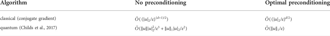
TABLE 1. Complexity results in Montanaro and Pallister (2016). The problem is a second order elliptical PDE, discretized with the finite element method, using piece-wise linear shape functions.

The complexity analysis was done both without preconditioning and with optimal preconditioning (i.e. PA = I), where a realistic preconditoning case lies in between these two extremes. The most important result in Table 1 is that, for fixed dimension d, no exponential quantum speed-up can be achieved, regardless of conditioning. The reason is that to compute $⟨r|x⟩$ up to precision ɛ requires $O(1/\sqrt{\epsilon })$ repetitions of the QLSA while performing quantum amplitude amplification (Montanaro and Pallister, 2016). Still, if d was allowed to vary, it may look as if the quantum solver is exponentially faster than classical (no curse of dimensionality). However, the authors warn that the $\tilde{O}$ notation hides terms that are independent of 1/ɛ but can vary with d, making it hard to say what kind of speed-up is achievable for variable dimensions. Furthermore, a classical random walk procedure can solve the Poisson equation in polynomial time, if the solution is required only at a particular point (Linden et al., 2020).

The runtimes in Table 1 scale with 1/ɛ, $|u{|}_l{‖u‖}_l$, where the last two quantities are respectively the Sobolev l-seminorm and l-norm of the analytical solution u and are indicative of the magnitudes up to the lth derivative of u. Therefore, for d relatively high, yet fixed, there can be a consistent polynomial speed-up for high precision problems and high second derivatives of the solution u(x). These considerations extend to higher-order finite elements, with the difference that higher-order Sobolev seminorms appear in the runtime. However, from a structural mechanics standpoint, elliptical problems reach at most d = 3, limiting the achievable polynomial speed-up.

It is important to carefully understand why, even considering a log(1/ɛ)-scaling algorithm, Montanaro and Pallister found out that quantum linear solvers cannot provide exponential speed-up. To do this, one should answer the questions identified by Aaronson in his ‘fine print’ for quantum linear algebra (Aaronson, 2015).

1. Can $\left|b\right.⟩$ be prepared in time O(log(1/ɛ)), starting from b? In general, this is a hard problem, but if f(x) in Eq. 21 is a polynomial or a function supported only on a few elements, the state $\left|b\right.⟩$ can indeed be prepared in time O(log(1/ɛ)) (Montanaro and Pallister, 2016).

2. Is there an algorithm for accessing the elements of A in time O(log(1/ɛ))? Yes. In fact, quantum linear solvers require a sparse matrix and a sparse access to the matrix. The second point means that there should be an algorithm that, given a row index r and another index i, it returns the column index and value of the ith non-zero element in A. Finite element matrices satisfy both these requirements, since they are sparse and, if the mesh is regular, sparse access can be obtained by the knowledge of the element’s degrees of freedom and by the connectivity matrix.

3. Is possible to apply efficient pre-conditioning to A? Yes, for instance through the quantum-SPAI technique proposed by Clader et al. (Clader et al., 2013).

4. Is it possible to measure the output in time O(log(1/ɛ))? Not in general. Especially, it is not the case for estimating properties such as $⟨r|u⟩$, where distinguishing between two quantum states that are ɛ-close to each other require $O(1/\sqrt{\epsilon })$ queries to the QLE algorithm (Montanaro and Pallister, 2016).

Thus, the mere fact of having to sample a solution almost always kills any quantum exponential speed-up. Still, Montanaro and Pallister specify that there are cases in which some properties of the solution may be tested with logarithmic sampling. One such property is periodicity, which suggests the possibility of an exponential speed-up when using quantum linear solvers for the sake of finding the vibration frequencies of a structure.

Also, an even more interesting point in Montanaro’s analysis is the fact that a possible exponential speed-up will not arise from a QLE algorithm, but from a clever choice of state preparation or measurement. In fact, replacing a QLE routine with a classical linear solver implies at worst a polynomial slowdown (Montanaro and Pallister, 2016).

3.1.5 NISQ solvers

So far, none of the work discussed concerns the implementation of algorithms on hardware. In the most abstract cases, parts of the algorithm are performed by oracles, which perform a certain function in given time complexity, but whose circuit structure is unknown. Other times the circuit is sketched at different levels of detail. Most notably for the Poisson case, Wang et al. showed the circuit of their algorithm and all its modules up to qubit operations (gates) (Wang et al., 2020c).

However, it is easy to realize that none of these algorithms can possibly run on quantum hardware either today or in the next few decades (Preskill, 2018). For instance, Wang demonstrates his algorithm to solve a minimal problem of a 4 × 4 Poisson matrix (Wang et al., 2020c) on the Sunway TaihuLight supercomputer, which acts as a quantum simulator (Chen et al., 2018). Interestingly, the authors also provide qubit and gate counts for this implementation, declaring 38 qubits and 800 gates. One should consider that the actual gate count is higher, since gates such as TOFFOLI and SWAP used in Wang et al. (2020c) must be expanded to native operations and all operations have to be mapped to actual hardware connectivity. Therefore, circuits of this size require quantum volumes that are beyond near-term capabilities by orders of magnitude. Consequently, other authors recently looked at the possibility to solve the Poisson equation with near-term techniques.

Wang et al. also proposed a way to solve the one-dimensional Poisson problem in NISQ, using circuits of O(poly log(1/ɛ)) operations (Wang et al., 2020b). Their main idea was that the gate-expensive Hamiltonian simulation can be bypassed if one is able to directly encode the inverse eigenvalues in the quantum state amplitudes. This is easily understood by recalling the expression of the solution of the $A\left|x\right.⟩=\left|b\right.⟩$ linear system

$\left|x\right.⟩=A^{-1}\left|b\right.⟩=\sum _j\frac{{\beta }_j}{{\lambda }_j}\left|u_j\right.⟩,$

where λ_j and $\left|u_j\right.⟩$ are the jth eigenvalue and eigenvector of A respectively and $\left|b\right.⟩={\sum }_{j=1}^N{\beta }_j\left|u_j\right.⟩$.

Importantly, the Poisson problem with homogeneous Dirichlet boundary conditions results in a matrix whose eigenvalues have an analytical expression, i.e.

${\lambda }_j=4N^2{\sin }^2\left(\frac{j\pi }{2N}\right),(37)$

where j ranges from 1 N to 2.

Wang et al. noticed that this Poisson matrix is also a Cartan matrix. The eigenvalues of Cartan matrices are also sines and they are related by the following product relation (Damianou, 2014)

$2^{2^{n+1}-2}\prod _{j=1}^{2^n-1}{\sin }^2\left(\frac{j\pi }{2^{n+1}}\right)=2^n,(38)$

where n = log(N).

It is easy to see that the sine terms in the product are equal to the eigenvalues in Eq. 37 up to a constant term. Consequently, 1/λ_j can be written as a product of all other eigenvalues λ_k, for k ≠ j. Still, implementing Eq. 38 would require O(N) qubits, since every inverse eigenvalue depends on 2ⁿ − 1 others. The authors however used the periodicity of the discrete sines and some trigonometric relations to prove that 1/λ_j can be computed from Eq. 38 as product of only n − 2 sine terms. This allows the algorithm to be implemented in 3n qubits. Moreover, the sine expressions in Eq. 38 can be peformed straightforwardly as controlled R_y rotations.

Wang et al. also present the circuit for their algorithm, stating that the total cost expressed in one and two qubits gates is $\frac{5}{3}{n}^3$. Also, they mention that parallelization of the controlled R_y operations could further reduce the gate count to 10n², by adding n − 2 ancillary qubits. For a few (n < 10) qubit problems the required number of gates may fit the specifications of with NISQ devices. Nevertheless, one should keep in mind that both gate count and the declared time complexity of O(poly log(1/ɛ)) do not take into account the preparation of $\left|b\right.⟩$ and measurement of a scalar quantity of $\left|x\right.⟩$. Ultimately however, the real shortcoming of Wang’s algorithm to be of practical interest is that it is limited to the one-dimensional Poisson matrix with homogeneous Dirichlet boundary conditions. As shown in Huang and McColl (1997) the associated tridiagonal matrix can be inverted analytically removing the need of such a specialized numerical technique. Unfortunately, Wang et al. do not mention the possibility of extending their method to higher dimensions or different boundary conditions.

A different NISQ approach to the discrete Poisson problem is to use variational quantum algorithms to solve the underlying linear system (Liu H.-L. et al., 2021). In case of linear systems, the variational state is $\left|x\right.⟩=U(\mathit{\theta })\left|0\right.⟩$, where U(θ) is the ansatz (see Section 2.5) and the loss functions needs to be zero when $\left|x\right.⟩=A^{-1}\left|b\right.⟩$. A possible choice for such a loss function is then

$\mathcal{L}\left(\mathit{\theta }\right)=\langle x\left(\mathit{\theta }\right)|A^{†}A|x\left(\mathit{\theta }\right)\rangle -|\langle b|A|x\left(\mathit{\theta }\right)\rangle {|}^2.(39)$

In the Poisson case the matrix A is symmetric, therefore A^†A = A² and Eq. 39 becomes

$\mathcal{L}\left(\mathit{\theta }\right)=\langle x\left(\mathit{\theta }\right)|A^2|x\left(\mathit{\theta }\right)\rangle -|\langle b|A|x\left(\right.\left.\mathit{\theta }\right)\rangle {|}^2.(40)$

A necessary condition for advantage with VQAs is that the terms in Eq. 40 must be efficiently evaluated on a quantum computer and ideally must be hard to evaluate in classically. Bravo-Prieto et al. (2019) proved that the latter requirement is satisfied for loss functions such as that in Eq. 39. On the other hand, efficient quantum evaluation is possible only if the following two necessary conditions are met.

1. A and A² can be decomposed in O(poly log(N)) operators O_k

2. These operators are observables and have a simple tensor-product form.

Notice that we will talk here about observables as Hermitian operators, whose eigenvectors form an orthonormal basis for measurement.

Liu et al. show that A and A² for the 1-dimensional Poisson matrix fulfill both requirements. For the number of decomposition terms, one can recursively decompose A_m, with m being the number of qubits as

$A_m=\left[\begin{array}{cc}\hfill A_{m-1}\hfill & \hfill D_{m-1}\hfill \\ \hfill D_{m-1}^T\hfill & \hfill A_{m-1}\hfill \end{array}\right],(41)$

where

$D_{m-1}=\left[\begin{array}{cccc}\hfill 0\hfill & \hfill \dots \hfill & \hfill \hfill & \hfill 0\hfill \\ \hfill ⋮\hfill & \hfill \ddots \hfill & \hfill \hfill & \hfill ⋮\hfill \\ \hfill 0\hfill & \hfill \hfill & \hfill \hfill & \hfill \hfill \\ \hfill -1\hfill & \hfill 0\hfill & \hfill \dots \hfill & \hfill 0\hfill \end{array}\right](42)$

For example, the 1 and 2 qubit cases are

$A_1=\left[\begin{array}{cc}\hfill 2\hfill & \hfill -1\hfill \\ \hfill -1\hfill & \hfill 2\hfill \end{array}\right]=2I-{\sigma }_{+}-{\sigma }_{+};$

$\begin{array}{cc}\hfill A_2& =\left[\begin{array}{cccc}\hfill 2\hfill & \hfill -1\hfill & \hfill 0\hfill & \hfill 0\hfill \\ \hfill -1\hfill & \hfill 2\hfill & \hfill -1\hfill & \hfill 0\hfill \\ \hfill 0\hfill & \hfill -1\hfill & \hfill 2\hfill & \hfill -1\hfill \\ \hfill 0\hfill & \hfill 0\hfill & \hfill -1\hfill & \hfill 2\hfill \end{array}\right]\hfill \\ \hfill & =I\otimes A_1-{\sigma }_{+}\otimes {\sigma }_{-}-{\sigma }_{-}\otimes {\sigma }_{+},\hfill \end{array}$

where ${\sigma }_{+}=\left|0\right.⟩\left.⟨1\right|$ and ${\sigma }_{-}=\left|1\right.⟩\left.⟨0\right|$. By applying repeated tensor products of A_m−1 with the identity and adding the center off-diagonal terms for the mth case, A_m can be written as a sum of 2m + 1 terms.

The matrix A² can instead be split into the following two submatrices

$\begin{array}{cc}\hfill A_m^2& =\left[\begin{array}{cccccc}\hfill 5\hfill & \hfill -4\hfill & \hfill 1\hfill & \hfill \hfill & \hfill \hfill & \hfill 0\hfill \\ \hfill -4\hfill & \hfill 6\hfill & \hfill -4\hfill & \hfill 1\hfill & \hfill \hfill \\ \hfill 1\hfill & \hfill \ddots \hfill & \hfill \ddots \hfill & \hfill \ddots \hfill & \hfill \ddots \hfill & \hfill \hfill \\ \hfill \hfill & \hfill \ddots \hfill & \hfill \ddots \hfill & \hfill \ddots \hfill & \hfill \ddots \hfill & \hfill 1\hfill \\ \hfill \hfill & \hfill \hfill & \hfill 1\hfill & \hfill -4\hfill & \hfill 6\hfill & \hfill -4\hfill \\ \hfill 0\hfill & \hfill \hfill & \hfill \hfill & \hfill 1\hfill & \hfill -4\hfill & \hfill 5\hfill \end{array}\right]\hfill \\ \hfill & =\left[\begin{array}{cccccc}\hfill 6\hfill & \hfill -4\hfill & \hfill 1\hfill & \hfill \hfill & \hfill \hfill & \hfill 0\hfill \\ \hfill -4\hfill & \hfill 6\hfill & \hfill -4\hfill & \hfill 1\hfill & \hfill \hfill \\ \hfill 1\hfill & \hfill \ddots \hfill & \hfill \ddots \hfill & \hfill \ddots \hfill & \hfill \ddots \hfill & \hfill \hfill \\ \hfill \hfill & \hfill \ddots \hfill & \hfill \ddots \hfill & \hfill \ddots \hfill & \hfill \ddots \hfill & \hfill 1\hfill \\ \hfill \hfill & \hfill \hfill & \hfill 1\hfill & \hfill -4\hfill & \hfill 6\hfill & \hfill -4\hfill \\ \hfill 0\hfill & \hfill \hfill & \hfill \hfill & \hfill 1\hfill & \hfill -4\hfill & \hfill 6\hfill \end{array}\right]-\left[\begin{array}{cccccc}\hfill 1\hfill & \hfill \hfill & \hfill \hfill & \hfill \hfill & \hfill \hfill & \hfill \hfill \\ \hfill \hfill & \hfill 0\hfill & \hfill \hfill & \hfill \hfill & \hfill \hfill \\ \hfill \hfill & \hfill \hfill & \hfill \ddots \hfill & \hfill \hfill & \hfill \hfill & \hfill \hfill \\ \hfill \hfill & \hfill \hfill & \hfill \hfill & \hfill 0\hfill & \hfill \hfill \\ \hfill \hfill & \hfill \hfill & \hfill \hfill & \hfill \hfill & \hfill 0\hfill & \hfill \hfill \\ \hfill \hfill & \hfill \hfill & \hfill \hfill & \hfill \hfill & \hfill \hfill & \hfill 1\hfill \end{array}\right]\hfill \\ \hfill & =B_m-C_m.\hfill \end{array}(43)$

The matrix B_m in Eq. 43 is decomposed in the same fashion as A_m, while C_m is the sum of just two terms

$C_m=\underset{m}{\underbrace{{\sigma }_{+}{\sigma }_{-}\otimes \cdots \otimes {\sigma }_{+}{\sigma }_{-}}}+\underset{m}{\underbrace{{\sigma }_{-}{\sigma }_{+}\otimes \cdots \otimes {\sigma }_{-}{\sigma }_{+}}}(44)$

Overall, $A_m^2$ can be decomposed in 4m + 1 terms. Since both A and A² are decomposed in O(log(N)) operators, the first requirement for advantage is satisfied. Furthermore, Eq. 28 states that the d-dimensional Poisson equation is the sum of tensor products of the identity tensor with the one-dimensional matrix. Therefore, the d-dimensional Poisson problem with Dirichlet boundary conditions can be handled with the same operators as in the d = 1 case and specifically with d(2m + 1) of them for A and (d(2m + 1))² for A². However, while Liu et al. also give a decomposition for the Neumann, Robin and mixed boundary conditions in the d = 1 case, the authors claim that the {σ₊, σ₋} decomposition cannot be extended trivially to the multidimensional case with boundary conditions different than Dirichlet ones.

Still, the operators in A_m and B_m are not Hermitian and cannot be used as observables. Liu et al. notice however that they can be made symmetric by mapping them in the higher dimensional space of Bell states. For instance, one can consider the 2 × 2, 1 qubit case and build two new operators O₁₁ and O₁₂, such that

$\begin{array}{cc}\hfill O_{11}& =\left[\begin{array}{cc}\hfill 0\hfill & \hfill {\sigma }_{+}\hfill \\ \hfill {\sigma }_{+}^{†}\hfill & \hfill 0\hfill \end{array}\right]=\left|{\phi }_{11}^{+}\right.⟩\left.⟨{\phi }_{11}^{+}\right|-\left|{\phi }_{11}^{-}\right.⟩\left.⟨{\phi }_{11}^{-}\right|,\hfill \\ \hfill O_{12}& =\left[\begin{array}{cc}\hfill 0\hfill & \hfill {\sigma }_{-}\hfill \\ \hfill {\sigma }_{-}^{†}\hfill & \hfill 0\hfill \end{array}\right]=\left|{\phi }_{12}^{+}\right.⟩\left.⟨{\phi }_{12}^{+}\right|-\left|{\phi }_{12}^{-}\right.⟩\left.⟨{\phi }_{12}^{-}\right|,\hfill \end{array}(45)$

where $\left|{\phi }_{11}^{\pm }\right.⟩=\frac{1}{\sqrt{2}}(\left|00\right.⟩\pm \left|11\right.⟩)$, $\left|{\phi }_{12}^{\pm }\right.⟩=\frac{1}{\sqrt{2}}(\left|01\right.⟩\pm \left|10\right.⟩)$ are Bell states. By also defining $\left|\mathrm{0,1}\right.⟩$ and $\left|0,i1\right.⟩$ as the following 1-qubit states

$\begin{array}{cc}\hfill \left|\mathrm{0,1}\right.⟩& =\frac{1}{\sqrt{2}}\left(\left|0\right.⟩+\left|1\right.⟩\right),\hfill \\ \hfill \left|0,i1\right.⟩& =\frac{1}{\sqrt{2}}\left(\left|0\right.⟩+i\left|1\right.⟩\right),\hfill \end{array}(46)$

it is possible to evaluate the terms appearing in Eq. 40, such as

$\begin{array}{cc}\hfill \langle x\left(\mathit{\theta }\right)|{\sigma }_{+}|x\left(\mathit{\theta }\right)\rangle & =\left.⟨\mathrm{0,1}\right|\left.⟨x\left(\mathit{\theta }\right)\right|O_{11}\left|\mathrm{0,1}\right.⟩\left|x\left(\mathit{\theta }\right)\right.⟩-i\left.⟨0,i1\right|\left.⟨x\left(\mathit{\theta }\right)\right|O_{11}\left|0,i1\right.⟩\left|x\left(\mathit{\theta }\right)\right.⟩,\hfill \\ \hfill \langle x\left(\mathit{\theta }\right)|{\sigma }_{-}|x\left(\mathit{\theta }\right)\rangle & =\left.⟨\mathrm{0,1}\right|\left.⟨x\left(\mathit{\theta }\right)\right|O_{12}\left|\mathrm{0,1}\right.⟩\left|x\left(\mathit{\theta }\right)\right.⟩-i\left.⟨0,i1\right|\left.⟨x\left(\mathit{\theta }\right)\right|O_{12}\left|0,i1\right.⟩\left|x\left(\mathit{\theta }\right)\right.⟩.\hfill \end{array}(47)$

For higher matrix dimensions, measuring the expectation values of A_m and B_m requires to use similar operators as those in Eq. 45, but whose eigenvalues are entangled states in more than two qubits.

By measuring in the Bell basis, the second requirement is also satisfied. Indeed, Figure 5 shows that the measurement circuit in Liu H.-L. et al. (2021) is shallow and made by only one and two qubits gates. However, this circuit assumes full qubits connectivity, which is generally not available in current hardware. Therefore, the actual implementation on hardware will likely require SWAP gates to meet the design connectivity.

FIGURE 5

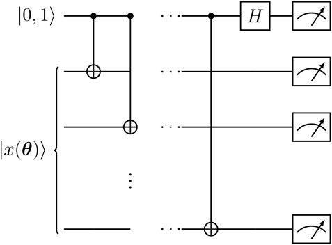
FIGURE 5. Circuit for measuring the state $\left|\mathrm{0,1}\right.⟩\left|x\left(\mathit{\theta }\right)\right.⟩$ in the Bell basis Liu H.-L. et al. (2021).

A final interesting remark regards the ansatz U(θ) chosen by Liu et al. for their simulations. This is the quantum alternating operator ansatz (QAOA) (Farhi et al., 2014; Hadfield et al., 2019), which consists of a layered circuit, each layer having only two parameters, corresponding to the evolution times of mixer and driver Hamiltonians. Liu H.-L. et al. (2021) chose the two Hamiltonians, such that their gate depth grows only linearly with the number of qubits. Furthermore, the results obtained on a quantum simulator show that the number of QAOA layers only needs to increase linearly with the number of qubits for fixed solution fidelity, resulting in a circuit that is overall suitable for NISQ hardware.

3.1.6 Quantum annealing

Srivastava and Sundararaghavan provided the first example of solving differential equations on a quantum annealer (Srivastava and Sundararaghavan, 2018). The motivation behind their work was that the functional minimization form of the differential problem can be written in terms of the discrete solution and solved as a combinatorial optimization problem. More precisely, the problem becomes a binary graph-coloring one, which is NP-hard.

As seen in Section 2.5.5, a quantum annealer finds the ground state of the Ising Hamiltonian, hereby reported for clarity

$H\left(\mathit{q}\right)=\sum _{i=1}^n{H}_i{q}_i+\sum _{\left(i,j\right)}{J}_{ij}{q}_i{q}_j$

The q_i binary variables encode the values of the discrete problem variables, while H_i and J_ij depend on problem data and boundary conditions.

For instance, consider the 1D Laplace problem with Dirichlet boundary conditions

$\left\{\begin{array}{c}\frac{{\mathrm{d}}^{2}u}{\mathrm{d}{x}^2}=0,\hfill \\ u\left(0\right)=u_0,\hfill \\ u\left(L\right)=u_L\hfill \end{array}\right.(48)$

where L is the length of the domain. The associated energy potential is

$\mathrm{\Pi }\left(u\right)={\int }_0^L\frac{1}{2}{\left(\frac{\mathrm{d}u}{\mathrm{d}x}\right)}^2\mathrm{d}x.(49)$

One can replace u(x) with the discrete solution

$u\left(x\right)\approx \sum _{i=1}^N{\phi }_i\left(x\right)a_i,(50)$

where φ_i(x) can be taken as the linear finite element shape functions in Eq. 36. In particular, finite element approximations are local, which fits well the fact that quantum annealers are only locally connected.

Considering only two elements (3 nodes) on the unit domain and substituting Eq. 50 in Eq. 49 leads to the discrete functional

$\mathrm{\Pi }\left(a_0,a_1,a_2\right)={\mathbf{a}}_1^T{\mathbf{s}}_1+{\mathbf{a}}_2^T{\mathbf{s}}_2,(51)$

where\

$\begin{array}{cc}\hfill {\mathbf{a}}_1& ={\left[a_0^2,a_1^2,a_0{a}_1,a_0,a_1\right]}^T\hfill \\ \hfill {\mathbf{a}}_2& ={\left[a_1^2,a_2^2,a_1{a}_2,a_1,a_2\right]}^T\hfill \\ \hfill {\mathbf{s}}_1& ={\mathbf{s}}_2={\left[\mathrm{1,1},-\mathrm{2,0,0}\right]}^T\hfill \end{array}.$

Srivastava and Sundararaghavan propose to associate every element to a local graph, to repeat this unit throughout the annealer’s graph and to form the global connections according to the finite element connectivity (Srivastava and Sundararaghavan, 2018). Every node i is associated with 3 qubits $q_j^i$, which in turn are mapped to 3 different values $v_{i_j}$ that the nodal solution can assume. Since $q_j^i=\pm 1$,

$a_i=\sum _{j=1}^3{v}_{i_j}\frac{q_i^j+1}{2}.(52)$

In this way, a_i can in principle assume 9 possible values. However, some of these values lead to invalid solutions and need to be penalized when writing the discrete potential.

Figure 6A shows the node graph used in Srivastava and Sundararaghavan (2018). This has associated H_l and ${\widehat{J}}_{lk}$ weights, which contibute to the Ising Hamiltonian. The aim of the nodal weights is to promote the boundary conditions as well as feasible values of the solution of the nodes. In case the PDE was not homogeneous, H_l and ${\widehat{J}}_{lk}$ would also account for the right hand side.

FIGURE 6

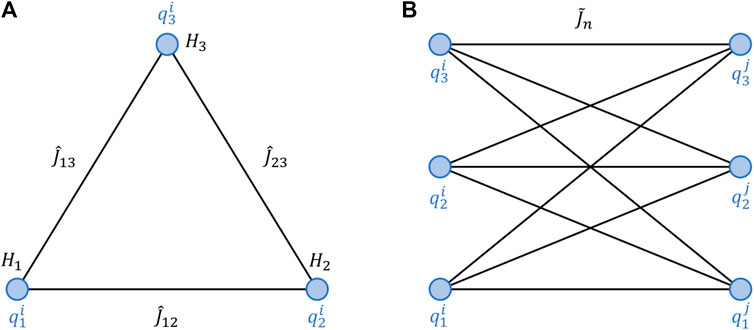
FIGURE 6. Generic node graph (A) and element graph (B) for the one dimensional Laplace equation in Srivastava and Sundararaghavan (2018) with the corresponding weigths of the Ising Hamiltonian.

Figure 6B shows instead the element graph for a single element, that is characterized by the matrix ${\tilde{J}}_n$. In the case of a 1D domain, the connection is between two adjacent nodes, each characterized by 3 qubits, therefore the element weight matrix ${\tilde{J}}^n$ is characterized by 9 linear equations

$\sum _{k=1}^3\sum _{l=1}^3{\left({\tilde{J}}^n\right)}_{kl}{q}_k^i{q}_l^j={\mathbf{a}}_n{\left(a_i,a_j\right)}^T{\mathbf{s}}_n,(53)$

where i and j are the nodes connected by element n.

Once H_l, ${\widehat{J}}_{lk}$ and ${({\tilde{J}}^n)}_{kl}$ are defined for every node and element, the weights in the transverse Ising Hamiltonian are defined and the quantum annealer can search for its ground state.

However, if a higher precision is required while spanning the same range of possible values, then more than 3 qubits would be required per node. In a realistic FE model with thousands of nodes this would require a high number of qubits and a high degree of connectivity, which may be beyond hardware capacity. Therefore Srivastava and Sundararaghavan proposed the so-called “box algorithm”. The main idea is to have the values $v_{i_j}$ centered around a value $u_i^c$ with distance r, thus

$v_{i_j}=u_i^c+r\left(j-2\right)(54)$

In this way, the nodal values are spaced around $u_i^c$ with radius r and for N nodes, all possible admissible values will be distributed on the surface of a N-dimensional box. The procedure consists in doing subsequent annealings until the desired precision r is met. After every annealing, $u_i^c$ and r are allowed to vary according to the following logic.

1. If $u_i^c\pm r$ for a certain i has lower potential than $u_i^c$, then the center is moved to that point

2. If $u_i^c$ is the point of minimum in the box, then r is reduced.

The procedure continues until r is below a threshold defined by the required solution precision. Also, Srivastava and Sundararaghavan (2018) show that this is a convergent process.

The graph-coloring and box algorithm is benchmarked against two truss problems, described by the equation

$\frac{\mathrm{d}}{\mathrm{d}x}\left(EA\frac{\mathrm{d}u}{\mathrm{d}x}\right)+f\left(x\right)=0,(55)$

where E(x) and A(x) are respectively the distributed axial stiffness and area, while f(x) is the distributed load over the truss. The first example is a truss with a discontinues cross-section at half length, while the second one is a tapered truss with distributed load. Both examples converge to the numerical FE solution using up to 6 elements. The authors also mention that a finer discretization would likely require a two-point version of the box technique, in order to better exploit the connectivity of the annealer.

3.2 Heat equation

The heat equation is another widely applicable mathematical model in solid mechanics, which can be used to predict temprerature profiles and heat concentrations in structural components.

Let the spatial domain be $\mathrm{\Omega }\subseteq {\mathbb{R}}^d$, and the temporal domain be $I\subseteq \mathbb{R}$. The solution u(x, t) satisfies the equation

$\frac{\partial u}{\partial t}=\frac{{\partial }^{2}u}{\partial x_1^2}+\cdots +\frac{{\partial }^{2}u}{\partial x_d^2}={\nabla }^{2}u,\mathbf{x}={\left[x_1,\dots ,x_d\right]}^{\top }\in \mathrm{\Omega },t\in \left[0,T\right](56)$

and the differential problem is completed once the boundary and initial conditions are also specified.

For problems relevant in structural mechanics, the problems are at most three-dimensional. Also, one needs to account for the material’s thermal diffusivity, which is in general a tensor $\mathcal{A}\left(\mathbf{x}\right)\in {\mathbb{R}}^{d\times d}$, with entries depending on x. From here onwards however, the material is assumed isotropic and homogeneous, therefore the thermal diffusivity becomes a constant scalar α and

$\frac{\partial u}{\partial t}=\alpha \sum _{i\le 3}\frac{{\partial }^{2}u}{\partial x_i^2}.(57)$

3.2.1 Comparison of classical and gate-based quantum methods

A comprehensive study on quantum solvers for the heat equation was conducted by Linden et al. (Linden et al., 2020). Specifically, the authors compared 5 classical and 5 quantum methods in terms of their theoretical runtimes to approximate the temperature integrated over a region S ⊆Ω, up to precision ɛ with 99% success probability of the algorithm, i.e.

$\left|\tilde{H}-{\int }_{S}u\left(\mathbf{x},t\right)\mathrm{d}\mathbf{x}\right|\le \epsilon (58)$

where $\tilde{H}$ is the approximated temperature integral.

The discretization in time consists in first-order forward finite differences, while second-order centered finite differences are used for the space grid. This scheme is also called forward time centered space or FTCS, for short. Therefore Eq. 57 becomes the finite difference equation

$\frac{\tilde{u}\left(\mathbf{x},t+\mathrm{\Delta }t\right)-\tilde{u}\left(\mathbf{x},t\right)}{\mathrm{\Delta }t}=\frac{\alpha }{{\left(\mathrm{\Delta }x\right)}^2}\sum _{i=1}^d\tilde{u}\left(x_1,\dots ,x_i+\mathrm{\Delta }{x}_i,\dots ,x_d,t\right)-2\tilde{u}\left(x_1,\dots ,x_i,\dots ,x_d,t\right)+\tilde{u}\left(x_1,\dots ,x_i-\mathrm{\Delta }{x}_i,\dots ,x_d,t\right),(59)$

where Δt = T/M, M being the number of time intervals, while Δx = L/N, assuming equal length L for each dimension and division in N intervals. Furthermore, $\tilde{u}$ is the approximation of u due to the finite difference discretization.

By grouping the values of $\tilde{u}$ at the same time step, Eq. 59 can be rewritten as

$\tilde{u}\left(\mathbf{x},t+\mathrm{\Delta }t\right)=\left(1-\frac{2d\alpha \mathrm{\Delta }t}{{\left(\mathrm{\Delta }x\right)}^2}\right)\tilde{u}\left(\mathbf{x},t\right)+\frac{\alpha \mathrm{\Delta }t}{{\left(\mathrm{\Delta }x\right)}^2}\sum _{i=1}^d\tilde{u}\left(x_1,\dots ,x_i+\mathrm{\Delta }{x}_i,\dots ,x_d,t\right)+\tilde{u}\left(x_1,\dots ,x_i-\mathrm{\Delta }{x}_i,\dots ,x_d,t\right).(60)$

Also, by defining ${\tilde{\mathbf{u}}}_i$ as the solution at time step t_k, k = {1, …M}, Eq. 60 can be written in vector form as

${\tilde{\mathbf{u}}}_{k+1}=\mathcal{L}{\tilde{\mathbf{u}}}_k,(61)$

where $\mathcal{L}$ is the linear operator on the right-hand side of Eq. 60.

The classical solvers studied by Linden for this problem are the following.

1. Single linear system approach with conjugate gradient. Eq. 61 can be seen as a unique linear system, for the solution at subsequent times. In fact, if $\mathbf{u}={[{\mathbf{u}}_1,\dots {\mathbf{u}}_M]}^T$, $\mathbf{f}={[\mathcal{L}{\mathbf{u}}_0,\mathbf{0},\dots ,\mathbf{0}]}^T$ and u₀ is the initial condition in discrete space, then

$A\mathbf{u}=\mathbf{f},(62)$

where

$A=\left[\begin{array}{ccccc}\hfill I\hfill & \hfill 0\hfill & \hfill 0\hfill & \hfill \dots \hfill & \hfill 0\hfill \\ \hfill -\mathcal{L}\hfill & \hfill I\hfill & \hfill 0\hfill & \hfill \hfill & \hfill 0\hfill \\ \hfill 0\hfill & \hfill \ddots \hfill & \hfill \ddots \hfill & \hfill \ddots \hfill & \hfill ⋮\hfill \\ \hfill ⋮\hfill & \hfill \ddots \hfill & \hfill -\mathcal{L}\hfill & \hfill I\hfill & \hfill 0\hfill \\ \hfill 0\hfill & \hfill \dots \hfill & \hfill 0\hfill & \hfill -\mathcal{L}\hfill & \hfill I\hfill \end{array}\right](63)$

Linden et al. (2020) suggest to use the conjugate gradient method to solve the sparse linear system in Eq. 62 in linear time. More accurately however, one should resort to a variation of this method such as the biconjugate gradient stabilized method (BiCGSTAB) (van der Vorst, 1992), which still runs in linear time, in order to account for the asymmetry of A.

2. Time-stepping from initial condition. This is a matrix-vector multiplication problem. In fact, Eq. 61 can be expanded up to u₀ as

${\tilde{\mathbf{u}}}_{\mathbf{k}}={\mathcal{L}}^k{\mathbf{u}}_{\mathbf{0}}.(64)$

Then, the approximate solution at time t_k = kΔt is obtained by k successive multiplications of $\mathcal{L}$ to u₀.

3. Time-stepping using the Fast Fourier Transform (FFT). For the FTCS scheme, the matrix $\mathcal{L}$ in d dimensions has the expression (Linden et al., 2020)

$\mathcal{L}=I_N^{\otimes d}+\frac{\alpha \mathrm{\Delta }t}{{\left(\mathrm{\Delta }x\right)}^2}\sum _{j=1}^d{I}_N^{\otimes \left(j-1\right)}\otimes H\otimes I_N^{\otimes \left(d-j\right)},(65)$

where I_N is the identity matrix of dimension N. Also,

$H=\left[\begin{array}{ccccc}\hfill -2\hfill & \hfill 1\hfill & \hfill \hfill & \hfill \hfill & \hfill 1\hfill \\ \hfill 1\hfill & \hfill -2\hfill & \hfill 1\hfill & \hfill \hfill \\ \hfill \hfill & \hfill 1\hfill & \hfill \ddots \hfill & \hfill \ddots \hfill & \hfill \hfill \\ \hfill \hfill & \hfill \hfill & \hfill \ddots \hfill & \hfill \ddots \hfill \\ \hfill 1\hfill & \hfill \hfill & \hfill \hfill & \hfill 1\hfill & \hfill -2\hfill \end{array}\right](66)$

which is a circulant matrix and can therefore be diagonalized by the Discrete Fourier Transform F. Since the circulant matrices operate on different dimensions, the matrix $\mathcal{L}$ is diagonalized by the tensor product of F, i.e. F^⊗d. Furthermore, H has eigenvalues ${\lambda }_j=-4{\sin }^2\left(\frac{j\pi }{N}\right)$, which can be used in combination with Eq. 65 to compute the eigenvalues of $\mathcal{L}$. Therefore,

$\mathcal{L}={\left(F^{\mathit{\otimes d}}\right)}^{-1}\mathrm{\Delta }{F}^{\otimes d},(67)$

where Λ is the diagonal matrix with the eigenvalues of $\mathcal{L}$ on the diagonal. Therefore the time stepping equation Eq. 64 becomes

${\tilde{\mathbf{u}}}_k={\left(F^{\mathit{\otimes d}}\right)}^{-1}{\mathrm{\Delta }}^k{F}^{\otimes d}{\mathbf{u}}_0.(68)$

Numerically, this consists in doing the Fast Fourier Transform (FFT) of u₀, multiplying the resulting vector by the kth powers of the eigenvalues of $\mathcal{L}$ and finally performing an inverse FFT.

4. Random walk. Eq. 60 can be seen in terms of stochastic quantities. In fact, introducing $s=\frac{\alpha \mathrm{\Delta }t}{{(\mathrm{\Delta }x)}^2}$, this equation can be rewritten as

$\tilde{u}\left(\mathbf{x},t+\mathrm{\Delta }t\right)=\left(1-2ds\right)\tilde{u}\left(\mathbf{x},t\right)+\sum _{i=1}^{d}s\tilde{u}\left(x_1,\dots ,x_i+\mathrm{\Delta }{x}_i,\dots ,x_d,t\right)+s\tilde{u}\left(x_1,\dots ,x_i-\mathrm{\Delta }{x}_i,\dots ,x_d,t\right).(69)$

It is easy to see that if s ≤ 1/(2d), Eq. 69 can be thought of as a stochastic process. In fact, the temperature $\tilde{u}$ at each time is determined by those at the preceding time step on the surrounding d-dimensional lattice with probabilities determined by s. In this sense the FTCS equation is a random walk, where the position is the approximate temperature $\tilde{u}$.

5. Fast random walk. The standard random walk samples for all m time steps, each sample requiring O(d log(N)) time, for a total time of O(Md log(N)). A speed-up can be achieved with respect to this standard technique. First, sample from the intial distribution in O(d log(N)) time and then compute the number of steps in each dimension d and the number of positive/negative increments in every dimension, by sampling two binomial distributions in time O(log(M)) (Linden et al., 2020). The improved runtime is O(d(log(M) + log(N))).

For their comparison, Linden et al. discussed how quantum subroutines could speed-up the classical numerical algorithms for the heat equation. In the case of quantum algorithms, the final solution state $\left|\widetilde{\stackrel{̃}{u}}\right.⟩$ approximates $\left|\tilde{u}\right.⟩$, that is the quantum state representation of u of the FTCS equation. Starting from $\left|\widetilde{\stackrel{̃}{u}}\right.⟩$, the approximate integrated temperature $\tilde{H}$ in region S ⊆ Ω can be calculated up to precision ɛ using numerical quadrature, i.e.

$\left|{\int }_{S}u\left(\mathbf{x},t\right)\mathrm{d}\mathbf{x}-{\left(\mathrm{\Delta }x\right)}^d\sum _{\mathbf{x}\in G\cap S}{\widetilde{‖\stackrel{̃}{u}‖}}_{2}w\left(\mathbf{x}\right)⟨\mathbf{x},t|\widetilde{\stackrel{̃}{u}}⟩\right|\le \epsilon ,(70)$

where G is the d-dimensional grid in the domain Ω, ${\widetilde{‖\stackrel{̃}{u}‖}}_2$ is the numerically estimated norm of $\tilde{u}$ and w(x) are weights that depend on the specific numerical quadrature scheme.

The 5 quantum algorithms considered in (Linden et al., 2020) are listed below. The reader may notice that this list does not include the time-optimal quantum algorithm for ordinary differential equations proposed by Berry et al. (2017). However Linden et al. state that such method may have a cost higher than using a QLSA, even though the dependency with d is better for the quantum ODE solver (Linden et al. (2020); Appendix A).

1. Quantum linear solver. A quantum algorithm for linear systems can be used to solve Au = r, with matrix A defined in Eq. 63. Linden et al. utilized the algorithm in (Chakraborty et al., 2019), that is logarithmically dependent on precision. Even though this method requires the matrix to be Hermitian, it can still be applied to the FTCS-discretized heat equation by solving for

$\left[\begin{array}{cc}\hfill 0\hfill & \hfill A\hfill \\ \hfill A^{†}\hfill & \hfill 0\hfill \end{array}\right]\left[\begin{array}{c}\hfill 0\hfill \\ \hfill \mathbf{u}\hfill \end{array}\right]=\left[\begin{array}{c}\hfill \mathbf{f}\hfill \\ \hfill 0\hfill \end{array}\right]$

2. Fast forwarded quantum walk method. Quantum walks are a form of random walks that can be performed with unitary operations on quantum states (Ambainis, 2004). The first results in quantum walks showed how these could simulate random walks quadratically faster in the limit behavior (for a number of time-steps going to infinity). However, one is generally interested in the dynamics of the heat equation, other than its steady state. Using the quantum walk fast-forwarding algorithm of Apers and Sarlette (Apers and Sarlette, 2018), allows to have quadratic speed-up even when simulating a random walk at intermediate times, making it applicable to the heat equation.

3. Coherent diagonalisation. The operator ${\mathcal{L}}^k$ in Eq. 64 can be diagonalized exponentially faster using QFT instead of FFT. Ahead of measuring, one wants to reproduce the state

$\left|u_k\right.⟩={\mathcal{L}}^k\left|u_0\right.⟩,(71)$

where it is assumed that $\left|u_0\right.⟩$ can be prepared (Linden et al., 2020). If Φ is the Quantum Fourier Transform (QFT) operator, then

$\left|u_k\right.⟩={\mathrm{\Phi }}^{†}{\mathrm{\Lambda }}^k\mathrm{\Phi }\left|u_0\right.⟩,(72)$

where Λ is the same matrix appearing in Eq. 67. Therefore $\left|u_k\right.⟩$ can be prepared following these steps.

a. Prepare $\left|u_0\right.⟩$.

b. Apply QFT.

c. Apply the Λ^k operator. This is not unitary in general, but it can be implemented by using an ancilla qubit, applying a rotation controlled on the $\mathrm{\Phi }\left|u_0\right.⟩$ state, measuring and post-selecting (Linden et al., 2020).

d. Apply the inverse QFT.

4. Random walk with amplitude estimation. The random walk technique can be ran O(1/ɛ) faster using amplitude estimation. In fact, approximating ∫_Su(x)dx requires O(1/ɛ²) repetitions of the classical random walk due to the Chernoff bound. However, assume there is a Boolean function f(s) such that

$f\left(s\right)=\left\{\begin{array}{cc}0\hfill & \mathrm{i}\mathrm{f}\mathbf{x}\notin S\hfill \\ 1\hfill & \mathrm{i}\mathrm{f}\mathbf{x}\in S\hfill \end{array}\right.(73)$

at the end of the random walk. If f can be encoded as an oracle, then quantum amplitude estimation can estimate Pr(f(s) = 1) in O(1/ɛ) time. This can be directly used to compute ∫_Su(x)dx.

5. Fast random walk with amplitude estimation. In the same way as in standard random walks, amplitude estimation can be applied to the fast random walk technique (see classical methods).

Table 2 shows the time complexities of all classical and quantum methods analyzed in Linden et al. (2020). In general, the classical FFT diagonalization technique scores the best complexity for the one-dimensional heat equation, while fast random walks with quantum amplitude estimation have the lowest runtime for d ≤ 2. However, both of these techniques work only for hyper-rectangular domains, for which the heat equation has an analytical solution in terms of Fourier components (Haberman, 2014). Still, the amplitudes of these modes are integrals, often computed numerically. Depending on the initial condition u₀ and its Fourier decomposition, one may need to estimate a high number of integrals, in which case the methods for rectangular regions may still be meaningful.

TABLE 2

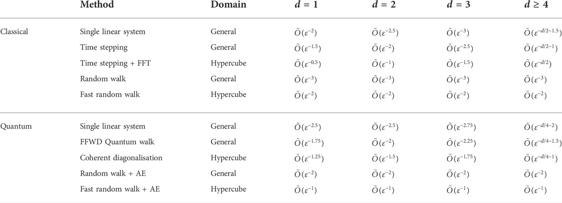
TABLE 2. Runtime comparison of classical and quantum methods for solving the FTCS heat equation (Linden et al., 2020). All runtimes are expressed in terms of terms of spatial dimensions d and error ɛ on the estimated temperature integral. The $\tilde{O}$ notation hides polylogarithmic factors in the complexity. Adapted from Linden et al. (2020).

On the other hand, quantum algorithms can still be faster even on generic domains. In fact, except for d = 1 where the classical time-stepping technique has lowest runtime, standard random walks with quantum amplitude estimation are as fast (d = 2) or slightly faster (d = 3).

However, Table 2 also shows that no quantum exponential speed-up is possible. This happens even when some of the underlying quantum subroutines are ‘exponentially faster’ than their classical counterparts, as in the case of linear solvers. However, as showed by Montanaro for elliptical problems discretized by FEM, obtaining a scalar quantity requires O(poly(1/ɛ)) samples of the final quantum state (Montanaro and Pallister, 2016).

Finally, Table 2 shows that methods using a quantum algorithms for linear system are never faster than the best classical algorithm for d < 5, be it for rectangular or generic domains. Thus, one should be aware of this limitation, if aiming for a speed-up to solve the heat equation in a 3- or lower-dimensional space.

3.2.2 Quantum annealing

Another way to use quantum computing for solving the heat equation was proposed by Pollachini et al. (Pollachini et al., 2021). Their approach involved the use of quantum annealing in a quantum-classical loop, allowing the method to be implemented on DWave quantum annealers and solving the heat equation on a 9 × 9 grid.

The equation considered is

$k\left(\frac{{\partial }^{2}u}{\partial x_1^2}+\frac{{\partial }^{2}u}{\partial x_2^2}\right)+f\left(x_1,x_2\right)=0,(74)$

which describes the steady state of the temperature distribution on a 2D domain with source term f(x₁, x₂). Eq. 74 is actually a diffusion-reaction equation instead of a heat equation, where u(x₁, x₂) is the equilibrium temperature and f(x₁, x₂) is a distributed heat flux. Dirichlet conditions were used at the boundary.

Eq. 74 is discretized using centered finite differences in the usual way and the problem reduces to solving a linear system Au = f, where $f_i=f(x_1^{(i)},x_2^{(i)})\forall i\in G$, where G is the space grid.

Quantum annealers can solve problems that can be expressed as QUBO problems. In the case of linear systems, the quadratic Hamiltonian

$H\left(\mathbf{u}\right)={\left(A\mathbf{u}-\mathbf{f}\right)}^{\top }\left(A\mathbf{u}-\mathbf{f}\right)(75)$

has a ground state corresponding to the solution u = A⁻¹f (O’Malley and Vesselinov, 2016; Rogers and Singleton, 2020). Also, u_i can be restricted to the range [ − d_i, 2c_i − d_i) using the following mapping

$u_i=-d_i+c_i\sum _{r=0}^{R-1}\frac{q_r^i}{2^r},(76)$

where d_i and c_i are user-defined real numbers and $q_r^i$ are binary digits. In this way, u_i is associated to the binary string $q_r^i$ and the precision can be tuned by choosing d_i and c_i.

Eq. 76 can be substituted in Eq. 75, providing the Ising Hamiltonian

$H\left(\mathbf{q}\right)=\sum _{r=0}^{R-1}\sum _{i=0}^{N-1}{H}_r^i{q}_r^i+\sum _{r,s=0}^{R-1}\sum _{i,j=0}^{N-1}{J}_{rs}^{ij}{q}_r^i{q}_s^j,(77)$

where N is the number of nodes in the grid. Once the ground state of this Hamiltonian is obtained after annealing, the inverse of the mapping in Eq. 76 allows to reconstruct the solution.

Furthermore, Pollachini et al. provided a strategy to keep their algorithm hardware-feasible even for large problem dimensions. In fact, they proposed to use the iterative block Gauss-Seidel method, which consists in iteratively solving D blocks of dimension N/D instead of one N-dimensional linear system. For instance, taking D = 2

$\left[\begin{array}{cc}\hfill A_{11}\hfill & \hfill A_{12}\hfill \\ \hfill A_{21}\hfill & \hfill A_{22}\hfill \end{array}\right]\left[\begin{array}{c}\hfill {\mathbf{u}}_1\hfill \\ \hfill {\mathbf{u}}_2\hfill \end{array}\right]=\left[\begin{array}{c}\hfill {\mathbf{f}}_1\hfill \\ \hfill {\mathbf{f}}_2\hfill \end{array}\right].(78)$

Eq. 78 can be solved iteratively, by making an initial guess for u₂ as ${\mathbf{u}}_2^{(0)}$. Then, at time step k + 1,

$\left\{\begin{array}{cc}{A}_{11}{\mathbf{u}}_1^{\left(k+1\right)}\hfill & ={\mathbf{f}}_1-A_{12}{\mathbf{u}}_2^{\left(k\right)}\hfill \\ A_{22}{\mathbf{u}}_2^{\left(k+1\right)}\hfill & ={\mathbf{f}}_2-A_{21}{\mathbf{u}}_1^{\left(k\right)}\hfill \end{array}\right..(79)$

The quantum annealer takes care of solving each lower-dimensional linear systems in Eq. 79 and Gauss-Seidel iterations are repeated until convergence.

As mentioned, Pollachini et al. ran their algorithm on both DWave 2000Q and DWave Advantage quantum annealers (D-Wave, 2022). The source term f(x₁, x₂) was taken randomly and Eq. 74 was discretized on a 11 × 11 grid, corresponding to 9 internal points and a linear system with 81 unknowns. This is to date one of the largest linear systems solved (at least partially) on quantum hardware.

One of the issues that arised in the computations is a flattening of the error curve for increasing iterations of the block Gauss Seidel solver. This was attributed to saturating the floating-point precision achievable by a fixed number of qubits R. Indeed the authors fixed this issue by progressively shrinking the d_i range in Eq. 76, matching the same convergence curve as the classical Gauss-Seidel algorithm. However, increasing the number of qubits R per interval did not benefit the solution’s precision, likely due to an increase in hardware noise.

Despite the approach of Pollachini et al. being hardware-ready and verified, it is unclear whether it may provide an advantage. Furthermore, their method can only be applied to the steady-state problem. However, an alternative to solve the time-dependent within quantum annealing would be to perform a semi-discretization in space and then use the algorithm for systems of linear ODEs proposed in Zanger et al. (2021).

3.3 Wave equation

A third classical PDE is the wave equation, which describes the propagation of a perturbation through a medium. In solid mechaics, the wave equation can be used to model vibrations in structures or seismic wave propagation in soil.

The wave equation is written as

$\frac{{\partial }^{2}u}{\partial t^2}=c^2\sum _{i=1}^d\frac{{\partial }^{2}u}{\partial x_i^2},\mathbf{x}={\left[x_1,\dots ,x_d\right]}^{\top }\in \mathrm{\Omega },t\in \left[0,T\right],(80)$

where c is the wave propagation speed in the medium. As usual, the problem is fully determined once the solution at the boundary and two initial conditions are given.

Except for a few instances, where an analytical solution can be found through separation of variables or using the method of characteristics, the FDM and FEM are generally used to find an approximate solution of the wave equation. For instance, in the case of FDM, the Laplacian on the right hand side of Eq. 80 is discretized with centered finite differences and then a Runge-Kutta scheme allows to find the solution at subsequent time steps, starting from the initial conditions

$\left\{\begin{array}{cc}u\left(\mathbf{x},0\right)\hfill & =u_0\left(\mathbf{x}\right)\hfill \\ {\left.\frac{\partial u}{\partial t}\right|}_{t=0}\hfill & ={\dot{u}}_0\left(\mathbf{x}\right)\hfill \end{array}\right..(81)$

The exact runtimes of these classical methods depend on the order of discretization r of the Laplacian, the choice of the time-stepping technique, etc. However, their asymptotic behavior is bounded from below as $\mathrm{\Omega }\left[T\mathrm{p}\mathrm{o}\mathrm{l}\mathrm{y}{\left(1/\epsilon \right)}^d\right]$, showing the curse of dimensionality already seen for the Poisson and heat equations.

Nevertheless, replacing classical linear algebra subroutines with quantum algorithms can remove the exponential dependency on d also when solving the wave equation. This was proved by Costa et al. (Costa et al., 2019), who showed how to turn Eq. 80 into a Schrödinger equation and solve it using Hamiltonian simulation.

For the sake of explanation, let the wave equation be one dimensional and take c = 1. As usual, the domain can be reduced to a grid of spacing Δx on which the Laplacian on the right hand side of Eq. 80 can be approximated. The number of gridpoints used for the finite difference approximation determines the order r of the discrete Laplacian L^(r) and the discretization error $‖\frac{1}{{(\mathrm{\Delta }x)}^2}{L}_i^{(r)}-{\nabla }^2(x^{(i)})‖$, which scales as $O\left({(\mathrm{\Delta }x)}^r\right)$. For instance, the standard centered difference scheme uses r = 2, such that

$\frac{1}{{\left(\mathrm{\Delta }x\right)}^2}{L}^{\left(2\right)}u\left(x^{\left(i\right)}\right)=\frac{u\left(x^{\left(i+1\right)},t\right)-2u\left(x^{\left(i\right)},t\right)+u\left(x^{\left(i-1\right)},t\right)}{{\left(\mathrm{\Delta }x\right)}^2}.(82)$

Furthermore, if one sees the grid that discretizes Ω as a graph G_Δx of $\left|V\right|$ vertices x⁽ⁱ⁾ and $\left|E\right|$ edges x⁽ⁱ⁺¹⁾ − x⁽ⁱ⁾, the discrete Laplacian can be thought of as a matrix L^(r)(G_Δx) defined on this graph.

Keeping r = 2, Eq. 80 becomes

$\frac{{\partial }^2\mathbf{u}}{\partial t^2}=\frac{1}{{\left(\mathrm{\Delta }x\right)}^2}{L}^{\left(2\right)}\mathbf{u},(83)$

where u = [u₁, u₂, …, u_N] and N is the number of vertices.

Now, assume that a matrix B exists, such that BB^† = L. One can then write

$\frac{\mathrm{d}}{\mathrm{d}t}\left[\begin{array}{c}\hfill {\mathbf{u}}_V\hfill \\ \hfill {\mathbf{u}}_E\hfill \end{array}\right]=-\frac{i}{\mathrm{\Delta }x}\left[\begin{array}{cc}\hfill 0\hfill & \hfill B\hfill \\ \hfill B^{†}\hfill & \hfill 0\hfill \end{array}\right]\left[\begin{array}{c}\hfill {\mathbf{u}}_V\hfill \\ \hfill {\mathbf{u}}_E\hfill \end{array}\right],(84)$

where u_V = u and u_E are additional variables associated to the edges of the graph G.

Deriving Eq. 84 with respect to time, one obtains

$\frac{{\mathrm{d}}^2}{\mathrm{d}{t}^2}\left[\begin{array}{c}\hfill {\mathbf{u}}_V\hfill \\ \hfill {\mathbf{u}}_E\hfill \end{array}\right]=-\frac{1}{{\left(\mathrm{\Delta }x\right)}^2}\left[\begin{array}{cc}\hfill B{B}^{†}\hfill & \hfill 0\hfill \\ \hfill 0\hfill & \hfill B^{†}B\hfill \end{array}\right]\left[\begin{array}{c}\hfill {\mathbf{u}}_V\hfill \\ \hfill {\mathbf{u}}_E\hfill \end{array}\right],(85)$

which shows that, if BB^† = L, then u_V both evolves according to the Schrödinger equation (Eq. 84) and it is the solution of the original wave equation.

For an order 2 Laplacian, the B matrix is the graph signed incidence matrix. If one assigns random orientations to the edges of graph G_Δx, then

$B_{ij}=\left\{\begin{array}{cc}\sqrt{W_{ij}}\hfill & \mathrm{i}\mathrm{f}\mathrm{e}\mathrm{d}\mathrm{g}\mathrm{e}j\mathrm{s}\mathrm{e}\mathrm{l}\mathrm{f}-\mathrm{l}\mathrm{o}\mathrm{o}\mathrm{p}\mathrm{s}\mathrm{i}\mathrm{n}\mathrm{v}\mathrm{e}\mathrm{r}\mathrm{t}\mathrm{e}\mathrm{x}i\hfill \\ \sqrt{W_{ij}}\hfill & \mathrm{i}\mathrm{f}\mathrm{v}\mathrm{e}\mathrm{r}\mathrm{t}\mathrm{e}\mathrm{x}i\mathrm{i}\mathrm{s}\mathrm{a}\mathrm{s}\mathrm{o}\mathrm{u}\mathrm{r}\mathrm{c}\mathrm{e}\mathrm{o}\mathrm{f}\mathrm{e}\mathrm{d}\mathrm{g}\mathrm{e}j\hfill \\ -\sqrt{W_{ij}}\hfill & \mathrm{i}\mathrm{f}\mathrm{v}\mathrm{e}\mathrm{r}\mathrm{t}\mathrm{e}\mathrm{x}i\mathrm{i}\mathrm{s}\mathrm{a}\mathrm{s}\mathrm{i}\mathrm{n}\mathrm{k}\mathrm{o}\mathrm{f}\mathrm{e}\mathrm{d}\mathrm{g}\mathrm{e}j\hfill \\ 0\hfill & \text{otherwise}\hfill \end{array}\right.,(86)$

where W_ij are weights assigned to the edges of the graph. For instance, in case of the second order Laplacian, the graph is unweigthed (W_ij = 1 ∀i, j).

If the Laplacian has order r > 2, the graph theoretical interpretation of B is not as straightforward. Yet, Costa et al. (2019) discusses a general algebraic procedure to determine the incidence matrices for these higher order Laplacians and provides the entries for B and L^(r) up to order 10.

In order to solve 84, one can perform Hamiltonian simulation to an initial state and determine u_V at time t. In particular, Costa et al. employ the algorithm of Berry et al. (2015b) for sparse Hamiltonian simulation, that is optimal with respect sparsity, error and simulation time.

It is shown that Hamiltonian simulation for time t = T requires a number of gates g that is $\tilde{O}\left(T{d}^2{\left(T/\epsilon \right)}^{1/r}\right)$ and that the initial state can be prepared in time $\tilde{O}\left(\left(r/2+1\right)d^{5/2}l{\left(T/\epsilon \right)}^{1/r}\right)$, where l is a characteristic domain dimension. Most importantly, these runtimes show no exponential dependency on the dimension d, even though they do not include the time required to sample the output. Still, unless the full Hilbert space needs to be sampled, the measurement step would not reintroduce the curse of dimensionality, but just a O(1/ɛ) factor.

Thus, as seen for the Poisson and heat equations, the speed-up with respect to classical numerical solvers is exponential for variable dimensions, but at most polynomial if the dimension is fixed. What is interesting to notice though is that the homogeneous wave equation has the “quantum-appealing” characteristics of being interpreted as a Schrödinger equation and solved via Hamiltonian simulation. The same authors of Costa et al. (2019) notice that if Eq. 80 was treated as a second-order ODE, rather than a Schrödinger equation on an extended Hilbert space, it could be solved using the algorithm of Berry et al. (2017), but that would result in a quadratic slowdown with respect to using Hamiltonian Simulation.

The work of Costa had an important follow-up in Suau et al. (2021), where the authors studied the implementation, number of gates and actual runtime of Costa’s wave equation solver. As a benchmark problem, they took the simplest case of a 1-dimensional wave equation with homogeneous Dirichlet boundary conditions on the end points. However, Suau’s implementation slightly deviates from the original wave equation solver, since the authors replaced the optimal-complexity Hamiltonian simulation algorithm of Berry et al. (2015b) with the more common Lie-Trotter-Suzuki (LTS) product formula (Lloyd, 1996; Berry et al., 2006).

Suau et al. compute the number of gates and runtimes required for implementing their wave equation algorithm, choosing the following gate set

$\left\{U_1\left(\lambda \right),U_2\left(\lambda ,\varphi \right),U_3\left(\lambda ,\varphi ,\theta \right),CNOT\right\},(87)$

where.

$U_3\left(\lambda ,\varphi ,\theta \right)=\left[\begin{array}{cc}\hfill \cos \left(\frac{\theta }{2}\right)\hfill & \hfill -e^{i\lambda }\sin \left(\frac{\theta }{2}\right)\hfill \\ \hfill e^{i\varphi }\sin \left(\frac{\theta }{2}\right)\hfill & \hfill e^{i\lambda +\varphi }\cos \left(\frac{\theta }{2}\right)\hfill \end{array}\right](88)$

$U_2\left(\lambda ,\varphi \right)=U_3\left(\lambda ,\varphi ,\frac{\pi }{2}\right)(89)$

$U_1\left(\lambda \right)=U_3\left(\lambda ,\mathrm{0,0}\right)(90)$

$CNOT=\left[\begin{array}{cccc}\hfill 1\hfill & \hfill 0\hfill & \hfill 0\hfill & \hfill 0\hfill \\ \hfill 0\hfill & \hfill 1\hfill & \hfill 0\hfill & \hfill 0\hfill \\ \hfill 0\hfill & \hfill 0\hfill & \hfill 0\hfill & \hfill 1\hfill \\ \hfill 0\hfill & \hfill 0\hfill & \hfill 1\hfill & \hfill 0\hfill \end{array}\right](91)$

The runtime is obtained by converting the Hamiltonian simulation circuit to the gates in Eq. 87 and using the gate execution times provided by the manufacturer (IBM, 2019). A first interesting point is that the circuit in Suau et al. (2021) represents one of the few instances of a quantum PDE algorithm specified in terms ‘common’ gates (i.e. directly translatable to hardware).

The gate counts of Suau’s algorithm match the asymptotic (big-O) behavior of the wave equation solver for variable error, simulation time and number of gridpoints. What is most interesting however, is that the constants hidden in the big-O scaling are huge (10⁵–10⁸). This results in extremely high gate counts even just for solving the simplest possible instance of the wave equation. For instance, given a moderately interesting grid size of 10⁶ nodes, the quantum wave equation solver requires 10¹⁷ gates. Furthermore, the total runtime required for such a problem size is almost 1,000 calendar years (Suau et al., 2021). In terms of number of qubits, the solver requires roughly 70 logical qubits, where ‘logical’ means fully error corrected. As mentioned by Suau et al. (2021) however, full error correction for a logical qubit requires between 1,000 and 10,000 physical qubits, therefore vastly overshooting the NISQ hardware characteristics.

4 Nonlinear PDEs

Possibly the most computationally demanding tasks in computational mechanics are those related to solving nonlinear problems. The non linearities may be characteristics of the material, such as hysteresis, plasticity or damage, but also arise in case of large displacements or in the presence of contact. Whatever the cause, the classical numerical solution is generally iterative and consists in solving large linear system of equations in possibly many iterations.

Quantum algorithms for nonlinear PDEs are scarce up to present date, and no work focuses specifically on structural mechanics. However, Lubasch et al. (2020) and Kyriienko et al. (2021) both proposed techniques to solve generic (or quasi-generic) nonlinear PDEs. Both approaches consist in variationally training a parametrized circuit and on using a hybrid stratregy, whereby the quantum computer estimates the cost function terms and the classical one implements the optimization update. However, the two methods have substantial differences in how to encode the nonlinearities and on how to compute the cost function.

The algorithm of Lubasch is schematically represented in Figure 7. The encoding of nonlinear term in the cost function is performed via the quantum nonlinear processing unit (QNPU), which is a circuit meant to compute nonlinear functions of polynomial form that appear in the cost function. These can be written as

$u^{{\left(1\right)}^{*}}\prod _{j=1}^r{O}_j{u}^{\left(j\right)},(92)$

FIGURE 7

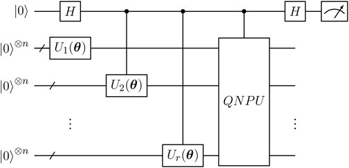
FIGURE 7. Scheme of the variational circuit in (Lubasch et al., 2020). The quantum nonlinear processing unit (QNPU) takes as input r copies of the solution vector, generated by the ansatz $U\left(\mathit{\theta }\right)$. Then, the QNPU applies the operators O_j in Eq. 92 as quantum operators. The circuit’s output comes from the measurements of the ancilla qubit and corresponds to the required cost function term.

Where the terms u⁽ⁱ⁾ are copies of the solution function and $u^{{(1)}^{*}}$ represents the complex conjugate of u⁽¹⁾. Furthermore, the O_j terms are different linear operators that are applied on different copies.

One can consider $\left|u^{(j)}\right.⟩$ as the properly normalized amplitude vector representation of u^(j). As usual, $\left|u^{(j)}\right.⟩$ can be a vector parametrized by means of an ansatz, i.e. $\left|u^{(j)}\right.⟩=U\left(\mathit{\theta }\right)\left|0\right.⟩$. The main idea of Lubasch’s approach is that the ansatz at a given optimization step can be used as many times as the number of solution copies required by Eq. 92 and the QNPU circuit applies the operators O_j and performs point-by-point multiplication depending on the specific nonlinear terms in the PDE.

The introduction of repeated input and the QNPU complicates the quantum circuit with respect to VQAs for linear problems. However, Lubasch et al. face the problem of circuit depth by encoding the quantum ansatz and the O_j operators as matrix product states (MPS) of bond dimension χ. This ensures that the circuits have $O(\mathrm{p}\mathrm{o}\mathrm{l}\mathrm{y}\left(\chi ,n\right))$, where $n={\log }_2\left(N\right)$ is the number of qubits. Furthermore, the number of parameters of an MPS ansatz is also polynomial in n and χ (Lubasch et al., 2020), preventing any curse of dimensionality.

The combination of multiple inputs and QNPU allows for an efficient way to reproduce nonlinearities. However, the QNPU block is strictly problem-dependent and it may not be trivial to implement, depending on the nonlinear expression.

A more versatile technique in this sense was proposed by Kyriienko et al, who considered the generic nonlinear problem

$F\left[{\left\{\frac{{\mathrm{d}}^m{u}_n}{\mathrm{d}{x}^m}\right\}}_{m,n},{\left\{u_n\left(x\right)\right\}}_n,x\right]=0,(93)$

here written for the 1D case.

Similarly to other near–term methods, this algorithm uses the variational principle to find the parametrized solution. However, a key difference in Kyriienko et al. (2021) is the fact that the solution is not represented as a discrete set of values on a grid, but as a function of x, thanks to the so–called quantum feature map. The concept of feature map originates from the machine learning literature and it consists in embedding the data into the model as parameters. Translating to quantum circuits, this means that x can be mapped to a 2ⁿ-dimensional space with a unitary operator U_ξ(x) parametrized through a nonlinear function ξ(x). Possibly the easiest instance of quantum feature map is

$U_{\xi }\left(x\right)=\underset{i=1}{\overset{n}{\otimes }}{R}_{Y,i}\left(\xi \left(x\right)\right),(94)$

where $R_{Y,i}=e^{-i\frac{\xi (x)}{2}{Y}_i}$ and Y_i is the Pauli Y gate applied to qubit i. A common choice is ξ(x) = arcsin(x), which means that x will be encoded in quantum amplitudes that are polynomials up to order 2ⁿ in $\left\{1,x,\sqrt{1-x^2}\right\}$ (Kyriienko et al., 2021).

As mentioned, the best approximation of u(x) is found variationally using the quantum circuit model. Therefore, Kyriienko’s technique also makes use of a circuit U_θ, whose parameters θ are varied to minimized an appropriate loss function. Overall, the parametrized quantum state whose amplitudes embed the tentative solution is

$\left|u_{\xi ,\theta }\left(x\right)\right.⟩=U_{\xi }\left(x\right)U_{\theta }\left|0\right.⟩.(95)$

In order to map between $\left|u_{\xi ,\theta }(x)\right.⟩$ and u(x), one needs also to specify an observable $\widehat{C}$, such that

$u\left(x\right)=\langle u_{\xi ,\theta }\left(x\right)|\widehat{C}|u_{\xi ,\theta }\left(x\right)\rangle .(96)$

Once, the parameters θ have been optimized, one can then reconstruct the approximate solution at a specific point x, by simply measuring the expectation value of $\widehat{C}$ under the state $\left|u_{\xi ,\theta }(x)\right.⟩$. This has the obvious advantage of not having to sample the entire 2ⁿ-dimensional Hilbert space, as it is necessary with the quantum algorithm based on amplitude encoding. Also, most of structural mechanics highly nonlinear problems are interesting with respect to the value of the solution or functions of it in just a small subset of points. For instance, this could be the case of probing the stress field at the crack tip of a fractured solid, by constructing $\widehat{C}$ such that it maps $\left|u_{\xi }(x)\right.⟩$ to the stress values.

In general, the training of U_θ requires the minimization of a loss function $L_{\theta }=L_{\theta }\left(\frac{{\mathrm{d}}^{m}u}{\mathrm{d}{x}^m},u,x\right)$ with respect to the parameters θ. Since the feature map is parametrized on x, the derivative $\frac{{\mathrm{d}}^{m}u}{\mathrm{d}{x}^m}$ in the loss function expression can be calculated by applying the parameter shift rule m times (Crooks, 2019; Mari et al., 2021). For m = 1

$\frac{\mathrm{d}u}{\mathrm{d}x}=\frac{1}{2}\sum _j\left(\langle u_{\xi ,j,\theta }^{+}|\widehat{C}|u_{\xi ,j,\theta }^{+}\rangle -\langle u_{\xi ,j,\theta }^{-}|\widehat{C}|u_{\xi ,j,\theta }^{-}\rangle \right),(97)$

where “+” and “−” symbolically represent the positive/negative x-shift and the sum is among all the parametrized gates composing the feature map. Suitable choices for L_θ can be the residual in Eq. 93 or the mean squared difference with respect to the exact solution, if this is available.

One clearly sees a parallel between Kyriienko’s method and training of neural networks. In the PDE case, during training, the function u is evaluated on a grid, which can be considered as the training dataset of a machine learning routine. Afterwards, the solution $u(x)=\langle u_{\theta }(x)|\widehat{C}|u_{\theta }(x)\rangle$ can be evaluated in other points in the domain, corresponding to the test dataset, in order to assess the validity of the model.

5 Discussion

The previous sections reviewed the literature of partial differential equations pertinent to structural mechanics. This analysis was divided into linear and nonlinear PDEs, which is a standard classification for differential problems. The first group includes the works about Poisson, heat and wave equations, while the second one deals with the methods to solve general nonlinear problems.

Linear problems can be solved using all different quantum paradigms, i.e. full gate-based, hybrid quantum computing and quantum annealing. In terms of the full-quantum gate-based primitives, such as quantum linear solvers, quantum Hamiltonian simulation etc, the Poisson, heat and wave equations can be solved with these quantum algorithms and inherit their complexities. However, the different character of the equations and the specific discretization determine which quantum routines are applicable and the extent of the advantage. For instance, quantum linear solvers are applicable to every linear PDE, both stationary and time-dependent, if the latter are written as a single linear system spanning multiple time steps. Nevertheless, the Poisson equation (on rectangular domains) with periodic boundary conditions is a favourite candidate for QLSAs, since the finite difference approximation of the Laplacian results in a circulant matrix that is diagonalized by the QFT (Cao et al., 2013; Wang et al., 2020c,b; Childs et al., 2021). This allows to do Hamiltonian simulation in the QLSA solving the Poisson equation exponentially faster than with non-circulant matrices.

On the other hand, heat and wave equations benefit more from different quantum subroutines. One hint to this is the evolutionary character of both equations, which means that linear system dimensions scale multiplicatively with respect to time grid size. Also, the time dependency seems to suggest the approach of semi-discretizing in space and then solving systems of ODEs with some Hamiltonian simulation algorithm. Indeed, this approach is ideal for the wave equation where Hamiltonian simulation solves the related graph problem in the higher dimensional space (Costa et al., 2019). On the other hand, the heat equation does not to benefit as much from quantum ODE solvers and the useful analysis of Linden et al. (2020) proves that minimum runtimes are achieved when accelerating a classical method (classical random walks) with amplitude acceleration.

Of course, all previous considerations hold for quantum subroutines that require error-corrected hardware. Still, near-term quantum techniques for linear PDEs exist under the umbrella of quantum annealing and variational quantum computing, even though the efforts in this sense are in their infancy. For PDEs in structural mechanics, only two quantum anneling algoritms have been proposed, namely for elliptical FE problems (Srivastava and Sundararaghavan, 2018) and for the stationary heat equation (Pollachini et al., 2021). Clearly, a first gap in this branch of literature are quantum annealing algorithms for evolutionary problems, such as heat and wave equations.

Also VQAs have just recently been applied to linear PDEs. Of course, the general literature on variational quantum computing is vast, but their use for PDEs have been limited to generic nonlinear problems (Lubasch et al., 2020; Kyriienko et al., 2021). However, there is still a lack of works for specific PDEs, even though such specialization is critical. For instance, Liu H.-L. et al. (2021) showed the relevance of the Poisson matrix in the context of VQAs. In fact, the discrete Poisson matrix can be decomposed in a poly-logarithmic number of observables, which is a necessary condition for advantage of variational PDE solvers.

For nonlinear problems, the matter of choosing a quantum primitive is not as straightforward, because all quantum operations are ultimately linear. The ways forward seem ultimately two, i.e linearization and application of existing quantum techniques or variational algorithms. Even though there exist research on linearization of nonlinear ODEs and use of QLSAs at each step (Liu J.-P. et al., 2021), all works on nonlinear PDEs relied so-far only on variational quantum computing. As it seems likely, this paradigm together with quantum annealing will likely be the only quantum alternative viable in the near term to solve PDEs, linear and nonlinear alike. However, there is currently a gap in literature about what can be expected from quantum computation for nonlinear PDEs in the error-corrected era. Having more insight in this direction would be extremely valuable, since nonlinear problems represent the most expensive and thus most interesting problems from a computational standpoint.

A final remark concerns extent of the overlap between quantum PDE and structural mechanics literature. In essence, this is currently limited to a single work on quantum annealing for truss problems (Srivastava and Sundararaghavan, 2018). In fact, the vast majority of literature focuses on ‘academic’ PDEs (Poisson, heat and wave) on hypercubic domains and for favorable boundary conditions. The exceptions are the methods for nonlinear equations, which essentially provide a framework from data encoding to solution, but ultimately leave the choice of critical hyperparameters to the user (Lubasch et al., 2020; Kyriienko et al., 2021). Of course, both sides of the spectrum project onto structural mechanics, but quantum computation still has to be tested against the specific and interesting problems in this field. What is even more surprising is that other disciplines away from quantum physics, yet heavily relying on numerical calculus (fluid mechanics, finance, etc) already applied quantum algorithms to their own cost-intensive problems. For instance, several works in fluid mechanics field used quantum subroutines to solve both the lattice Boltzmann (Mezzacapo et al., 2015; Todorova and Steijl, 2020; Budinski, 2021a) and the Navier-Stokes (Steijl and Barakos, 2018; Gaitan, 2020; Budinski, 2021b; Gaitan, 2021) equations. The hope is that structual mechanics will also explore the use of quantum algorithms to support expensive simulations, such as those involving material nonlinearities and large structural deformations.

Author contributions

GT reviewed the papers discussed in this work and wrote the manuscript. BC, MM, and MG all reviewed the work and provided critical feedback. RB followed the progress of the work and gave approval for publication.

Funding

This review work was provided by the Delft University of Technology.

Conflict of interest

The authors declare that the research was conducted in the absence of any commercial or financial relationships that could be construed as a potential conflict of interest.

Publisher’s note

All claims expressed in this article are solely those of the authors and do not necessarily represent those of their affiliated organizations, or those of the publisher, the editors and the reviewers. Any product that may be evaluated in this article, or claim that may be made by its manufacturer, is not guaranteed or endorsed by the publisher.

Footnotes

¹The “big Omega” notation expresses the asymptotic lower bound on the number of computational resources.

²A state or a subspace corresponding to a subset of basis states. For example, given the state $\left|a\right.⟩$, its projector is $\left|a\right.⟩\left.⟨a\right|$. By taking a second state $\left|b\right.⟩$, the projector operator can be applied to it, such that \begin{equation*} \left(\dyad{a} \right)\ket{b} = \ip{a}{b} \ket{a}, \end{equation*} which is a vector in the direction of $\left|a\right.⟩$, whose magnitude is the inner product between $\left|a\right.⟩$ and $\left|b\right.⟩$.

References

Aaronson, S. (2015). Read the fine print. Nat. Phys. 11, 291–293. doi:10.1038/nphys3272

CrossRef Full Text | Google Scholar

Aharonov, D., Jones, V., and Landau, Z. (2009). A polynomial quantum algorithm for approximating the jones polynomial. Algorithmica 55, 395–421. doi:10.1007/s00453-008-9168-0

CrossRef Full Text | Google Scholar

Aharonov, D., and Ta-Shma, A. (2003). “Adiabatic quantum state generation and statistical zero knowledge,” in Proceedings of the Thirty-Fifth Annual ACM Symposium on Theory of Computing, San Diego CA USA, June 9 - 11, 2003. doi:10.1145/780542.780546

CrossRef Full Text | Google Scholar

Ambainis, A. (2004). Quantum walks and their algorithmic applications. Int. J. Quantum Inf. 1, 507–518. doi:10.1142/s0219749903000383

CrossRef Full Text | Google Scholar

Ambainis, A. (2012). “Variable time amplitude amplification and quantum algorithms for linear algebra problems,” in 29th International Symposium on Theoretical Aspects of Computer Science (STACS 2012), Paris, France, February 29th - March 3rd, 2012. doi:10.4230/LIPIcs.STACS.2012.636

CrossRef Full Text | Google Scholar

An, D., and Lin, L. (2019). Quantum linear system solver based on time-optimal adiabatic quantum computing and quantum approximate optimization algorithm. United States: arXiv:1909.05500.

Google Scholar

An, D., Linden, N., Liu, J.-P., Montanaro, A., Shao, C., Wang, J., et al. (2020). Quantum-accelerated multilevel Monte Carlo methods for stochastic differential equations in mathematical finance. Quantum 5, 481. doi:10.22331/q-2021-06-24-481

CrossRef Full Text | Google Scholar

Apers, S., and Sarlette, A. (2018). Quantum fast-forwarding: Markov chains and graph property testing. United States: arXiv. 1804.02321.

Google Scholar

Benedetto, F. D. (1997). Preconditioning of block toeplitz matrices by sine transforms. SIAM J. Sci. Comput. 18, 499–515. doi:10.1137/s1064827595258335

CrossRef Full Text | Google Scholar

Benzi, M., and Tûma, M. (1999). A comparative study of sparse approximate inverse preconditioners. Appl. Numer. Math. 30, 305–340. doi:10.1016/s0168-9274(98)00118-4

CrossRef Full Text | Google Scholar

Berry, D. W., Ahokas, G., Cleve, R., and Sanders, B. C. (2006). Efficient quantum algorithms for simulating sparse Hamiltonians. Commun. Math. Phys. 270, 359–371. doi:10.1007/s00220-006-0150-x

CrossRef Full Text | Google Scholar

Berry, D. W., Childs, A. M., Cleve, R., Kothari, R., and Somma, R. D. (2014). “Exponential improvement in precision for simulating sparse Hamiltonians,” in Proceedings of the Forty-Sixth Annual ACM Symposium on Theory of Computing, New York, NY, USA, 31 May 2014- 3 June 2014, 283–292. doi:10.1145/2591796.2591854

CrossRef Full Text | Google Scholar

Berry, D. W., Childs, A. M., Cleve, R., Kothari, R., and Somma, R. D. (2015a). Simulating Hamiltonian dynamics with a truncated Taylor series. Phys. Rev. Lett. 114, 090502. doi:10.1103/PhysRevLett.114.090502

PubMed Abstract | CrossRef Full Text | Google Scholar

Berry, D. W., Childs, A. M., and Kothari, R. (2015b). “Hamiltonian simulation with nearly optimal dependence on all parameters,” in IEEE 56th Annual Symposium on Foundations of Computer Science, Berkeley, CA, USA, Oct. 17 2015 to Oct. 20 2015. doi:10.1109/focs.2015.54

CrossRef Full Text | Google Scholar

Berry, D. W., Childs, A. M., Ostrander, A., and Wang, G. (20172017). Quantum algorithm for linear differential equations with exponentially improved dependence on precision. Commun. Math. Phys. 356, 1057–1081. doi:10.1007/s00220-017-3002-y

CrossRef Full Text | Google Scholar

Brassard, G., Hoyer, P., Mosca, M., and Tapp, A. (2000). AMS Contemporary Mathematics in Quantum computation and quantum information. Editor J. SamuelLomonaco (Cambridge, New York: Cambridge University Press), 305, 53–74. doi:10.1090/conm/305/05215Quantum amplitude amplification and estimation

CrossRef Full Text | Google Scholar

Bravo-Prieto, C., LaRose, R., Cerezo, M., Subasi, Y., Cincio, L., and Coles, P. J. (2019). Variational quantum linear solver. United States: arXiv:1909.05820v2. 1909.

Google Scholar

Brenner, S. C., and Scott, L. R. (2010). “The mathematical theory of finite element methods. No. 15,” in Texts in applied mathematics (New York, NY: Springer), 3. nachdr.

Google Scholar

Budinski, L. (2021a). Quantum algorithm for the advection-diffusion equation simulated with the lattice Boltzmann method. Quantum Inf. process. 20, 57. doi:10.1007/s11128-021-02996-3

CrossRef Full Text | Google Scholar

Budinski, L. (2021b). Quantum algorithm for the Navier-Stokes equations. United States: rXiv:2103.03804. 2103.

Google Scholar

Buhrman, H., Cleve, R., Watrous, J., and de Wolf, R. (2001). Quantum fingerprinting. Phys. Rev. Lett. 87, 167902. doi:10.1103/PhysRevLett.87.167902

PubMed Abstract | CrossRef Full Text | Google Scholar

Cao, Y., Papageorgiou, A., Petras, I., Traub, J., and Kais, S. (2013). Quantum algorithm and circuit design solving the Poisson equation. New J. Phys. 15, 013021. doi:10.1088/1367-2630/15/1/013021

CrossRef Full Text | Google Scholar

Cerezo, M., Arrasmith, A., Babbush, R., Benjamin, S. C., Endo, S., Fujii, K., et al. (2021a). Variational quantum algorithms. Nat. Rev. Phys. 3, 625–644. doi:10.1038/s42254-021-00348-9

CrossRef Full Text | Google Scholar

Cerezo, M., Sone, A., Volkoff, T., Cincio, L., and Coles, P. J. (2021b). Cost function dependent barren plateaus in shallow parametrized quantum circuits. Nat. Commun. 12, 1791. doi:10.1038/s41467-021-21728-w

PubMed Abstract | CrossRef Full Text | Google Scholar

Chakrabarti, S., Krishnakumar, R., Mazzola, G., Stamatopoulos, N., Woerner, S., Zeng, W. J., et al. (2021). A threshold for quantum advantage in derivative pricing. Quantum 5, 463. doi:10.22331/q-2021-06-01-463

CrossRef Full Text | Google Scholar

Chakraborty, S., Gilyén, A., and Jeffery, S. (2019). “The power of block-encoded matrix powers: Improved regression techniques via faster Hamiltonian simulation,” in 46th International Colloquium on Automata, Languages, and Programming (ICALP 2019), Patras, Greece, 10 JULY 2019. doi:10.4230/LIPIcs.ICALP.2019.33

CrossRef Full Text | Google Scholar

Chen, Z.-Y., Zhou, Q., Xue, C., Yang, X., Guo, G.-C., Guo, G.-P., et al. (2018). 64-qubit quantum circuit simulation. Sci. Bull. 63, 964–971. doi:10.1016/j.scib.2018.06.007

CrossRef Full Text | Google Scholar

Childs, A. M., Kothari, R., and Somma, R. D. (2017). Quantum algorithm for systems of linear equations with exponentially improved dependence on precision. SIAM J. Comput. 46, 1920–1950. doi:10.1137/16m1087072

CrossRef Full Text | Google Scholar

Childs, A. M., Liu, J.-P., and Ostrander, A. (2021). High-precision quantum algorithms for partial differential equations. Quantum 5, 574. doi:10.22331/q-2021-11-10-574

CrossRef Full Text | Google Scholar

Ciliberto, C., Herbster, M., Ialongo, A. D., Pontil, M., Rocchetto, A., Severini, S., et al. (2018). Quantum machine learning: A classical perspective. Proc. R. Soc. A 474, 20170551. doi:10.1098/rspa.2017.0551

PubMed Abstract | CrossRef Full Text | Google Scholar

Clader, B. D., Jacobs, B. C., and Sprouse, C. R. (2013). Preconditioned quantum linear system algorithm. Phys. Rev. Lett. 110, 250504. doi:10.1103/PhysRevLett.110.250504

PubMed Abstract | CrossRef Full Text | Google Scholar

Costa, P. C. S., Jordan, S., and Ostrander, A. (2019). Quantum algorithm for simulating the wave equation. Phys. Rev. A . Coll. Park. 99, 012323. doi:10.1103/physreva.99.012323

CrossRef Full Text | Google Scholar

Crooks, G. E. (2019). Gradients of parameterized quantum gates using the parameter-shift rule and gate decomposition. United States: arXiv:1905.13311. 1905.

Google Scholar

D-Wave (2022). D-wave system documentation. Burnaby, Canada: D-Wave Systems Inc. Available at: https://docs.dwavesys.com/docs/latest/index.html.

Google Scholar

Damianou, P. A. (2014). A beautiful sine formula. Am. Math. Mon. 121, 120. doi:10.4169/amer.math.monthly.121.02.120

CrossRef Full Text | Google Scholar

Farhi, E., Goldstone, J., and Gutmann, S. (2014). A quantum approximate optimization algorithm. United States: arXiv. 1411.4028.

Google Scholar

Fontanela, F., Jacquier, A., and Oumgari, M. (2021). A quantum algorithm for linear pdes arising in finance. United States: arXiv. 1912.02753.

Google Scholar

Gaitan, F. (2020). Finding flows of a Navier–Stokes fluid through quantum computing. npj Quantum Inf. 6, 61. doi:10.1038/s41534-020-00291-0

CrossRef Full Text | Google Scholar

Gaitan, F. (2021). Finding solutions of the Navier-Stokes equations through quantum computing—Recent progress, a generalization, and next steps forward. Adv. Quantum Technol. 4, 2100055. doi:10.1002/qute.202100055

CrossRef Full Text | Google Scholar

Giovannetti, V., Lloyd, S., and Maccone, L. (2008a). Architectures for a quantum random access memory. Phys. Rev. A . Coll. Park. 78, 052310. doi:10.1103/physreva.78.052310

CrossRef Full Text | Google Scholar

Giovannetti, V., Lloyd, S., and Maccone, L. (2008b). Quantum random access memory. Phys. Rev. Lett. 100, 160501. doi:10.1103/physrevlett.100.160501

PubMed Abstract | CrossRef Full Text | Google Scholar

Golub, G. H., and van Loan, C. F. (2013). Matrix computations. fourth edn. Baltimore, Maryland, United States: JHU Press.

Google Scholar

Grover, L. K. (1996). “A fast quantum mechanical algorithm for database search,” in Annual ACM Symposyum on Theory Of Computing, Rome, Italy, June 20-24, 2022, 212–219.

CrossRef Full Text | Google Scholar

Grover, L. K. (19971997). Quantum mechanics helps in searching for a needle in a haystack. Phys. Rev. Lett. 79, 325–328. doi:10.1103/PhysRevLett.79.325

CrossRef Full Text | Google Scholar

Haberman, R. (2014). Applied partial differential equations with fourier series and boundary value problems. Harlow: Pearson.

Google Scholar

Hadfield, S., Wang, Z., O’Gorman, B., Rieffel, E., Venturelli, D., Biswas, R., et al. (2019). From the quantum approximate optimization algorithm to a quantum alternating operator ansatz. Algorithms 12, 34. doi:10.3390/a12020034

CrossRef Full Text | Google Scholar

Harrow, A. W., Hassidim, A., and Lloyd, S. (2009). Quantum algorithm for linear systems of equations. Phys. Rev. Lett. 103, 150502. doi:10.1103/physrevlett.103.150502

PubMed Abstract | CrossRef Full Text | Google Scholar

Heim, N., Ghosh, A., Kyriienko, O., and Elfving, V. E. (2021). Quantum model-discovery. United States: arXiv. 2111.06376.

Google Scholar

Huang, H.-Y., Bharti, K., and Rebentrost, P. (2021). Near-term quantum algorithms for linear systems of equations with regression loss functions. New J. Phys. 23, 113021. doi:10.1088/1367-2630/ac325f

CrossRef Full Text | Google Scholar

Huang, Y., and McColl, W. F. (1997). Analytical inversion of general tridiagonal matrices. J. Phys. A Math. Gen. 30, 7919–7933. doi:10.1088/0305-4470/30/22/026

CrossRef Full Text | Google Scholar

Kandala, A., Mezzacapo, A., Temme, K., Takita, M., Brink, M., Chow, J. M., et al. (2017). Hardware-efficient variational quantum eigensolver for small molecules and quantum magnets. Nature 549, 242–246. doi:10.1038/nature23879

PubMed Abstract | CrossRef Full Text | Google Scholar

Kato, T. (1950). On the adiabatic theorem of quantum mechanics. J. Phys. Soc. Jpn. 5, 435–439. doi:10.1143/jpsj.5.435

CrossRef Full Text | Google Scholar

Kingma, D. P., and Ba, J. (2015). “Adam: A method for stochastic optimization,” in 3rd International Conference on Learning Representations, ICLR 2015, San Diego, CA, USA, May 7-9, 2015.

Google Scholar

Kyriienko, O., Paine, A. E., and Elfving, V. E. (2021). Solving nonlinear differential equations with differentiable quantum circuits. Phys. Rev. A. Coll. Park. 103, 052416. doi:10.1103/physreva.103.052416

CrossRef Full Text | Google Scholar

Linden, N., Montanaro, A., and Shao, C. (2020). Quantum vs. classical algorithms for solving the heat equation. United States: arXiv:2004.06516v2. 2004.

Google Scholar

Liu, H.-L., Wu, Y.-S., Wan, L.-C., Pan, S.-J., Qin, S.-J., Gao, F., et al. (2021a). Variational quantum algorithm for the Poisson equation. Phys. Rev. A 104, 022418. doi:10.1103/PhysRevA.104.022418

CrossRef Full Text | Google Scholar

Liu, J.-P., Kolden, H. Ø., Krovi, H. K., Loureiro, N. F., Trivisa, K., Childs, A. M., et al. (2021b). Efficient quantum algorithm for dissipative nonlinear differential equations. Proc. Natl. Acad. Sci. U. S. A. 118, e2026805118. doi:10.1073/pnas.2026805118

PubMed Abstract | CrossRef Full Text | Google Scholar

Lloyd, S. (1996). Universal quantum simulators. Science 273, 1073–1078. doi:10.1126/science.273.5278.1073

PubMed Abstract | CrossRef Full Text | Google Scholar

Low, G. H., and Chuang, I. L. (2019). Hamiltonian simulation by qubitization. Quantum 3, 163. doi:10.22331/q-2019-07-12-163

CrossRef Full Text | Google Scholar

Lubasch, M., Joo, J., Moinier, P., Kiffner, M., and Jaksch, D. (2020). Variational quantum algorithms for nonlinear problems. Phys. Rev. A . Coll. Park. 101, 010301. doi:10.1103/physreva.101.010301

CrossRef Full Text | Google Scholar

Mari, A., Bromley, T. R., and Killoran, N. (2021). Estimating the gradient and higher-order derivatives on quantum hardware. Phys. Rev. A. Coll. Park. 103, 012405. doi:10.1103/physreva.103.012405

CrossRef Full Text | Google Scholar

McClean, J. R., Boixo, S., Smelyanskiy, V. N., Babbush, R., and Neven, H. (2018). Barren plateaus in quantum neural network training landscapes. Nat. Commun. 9, 4812. doi:10.1038/s41467-018-07090-4

PubMed Abstract | CrossRef Full Text | Google Scholar

McGeoch, C. C. (2020). Theory versus practice in annealing-based quantum computing. Theor. Comput. Sci. 816, 169–183. doi:10.1016/j.tcs.2020.01.024

CrossRef Full Text | Google Scholar

Mezzacapo, A., Sanz, M., Lamata, L., Egusquiza, I. L., Succi, S., Solano, E., et al. (2015). Quantum simulator for transport phenomena in fluid flows. Sci. Rep. 5, 13153. doi:10.1038/srep13153

PubMed Abstract | CrossRef Full Text | Google Scholar

Mocz, P., and Szasz, A. (2021). Toward cosmological simulations of dark matter on quantum computers. ApJ. 910, 29. doi:10.3847/1538-4357/abe6ac

CrossRef Full Text | Google Scholar

Montanaro, A., and Pallister, S. (2016). Quantum algorithms and the finite element method. Phys. Rev. A. Coll. Park. 93, 032324. doi:10.1103/physreva.93.032324

CrossRef Full Text | Google Scholar

Nielsen, M. A., and Chuang, I. L. (2010). Quantum computation and quantum information. 10th anniversary ed edn. Cambridge; New York: Cambridge University Press.

Google Scholar

O’Malley, D., and Vesselinov, V. V. (2016). Toq.jl: A high-level programming language for d-wave machines based on julia. In 2016 IEEE High Performance Extreme Computing Conference (HPEC), Waltham, MA, 13-15 Sept. 2016 1–7. doi:10.1109/HPEC.2016.7761616

CrossRef Full Text | Google Scholar

Patil, H., Wang, Y., and Krstić, P. S. (2022). Variational quantum linear solver with a dynamic ansatz. Phys. Rev. A . Coll. Park. 105, 012423. doi:10.1103/physreva.105.012423

CrossRef Full Text | Google Scholar

Pesah, A. (2020). Quantum algorithms for solving partial differential equations.

Google Scholar

Pollachini, G. G., Salazar, J. P. L. C., Góes, C. B. D., Maciel, T. O., and Duzzioni, E. I. (2021). Hybrid classical-quantum approach to solve the heat equation using quantum annealers. Phys. Rev. A . Coll. Park. 104, 032426. doi:10.1103/physreva.104.032426

CrossRef Full Text | Google Scholar

Preskill, J. (2018). Quantum computing in the NISQ era and beyond. Quantum 2, 79. doi:10.22331/q-2018-08-06-79

CrossRef Full Text | Google Scholar

Rogers, M. L., and Singleton, R. L. (2020). Floating-point calculations on a quantum annealer: Division and matrix inversion. Front. Phys. 8. doi:10.3389/fphy.2020.00265

CrossRef Full Text | Google Scholar

Shewchuk, J. R. (1994). An introduction to the conjugate gradient method without the agonizing pain. USA: Tech. rep.

Google Scholar

Somma, R. D., and Subaşı, Y. (2021). Complexity of quantum state verification in the quantum linear systems problem. PRX Quantum 2, 010315. doi:10.1103/prxquantum.2.010315

CrossRef Full Text | Google Scholar

Spall, J. (1992). Multivariate stochastic approximation using a simultaneous perturbation gradient approximation. IEEE Trans. Autom. Contr. 37, 332–341. doi:10.1109/9.119632

CrossRef Full Text | Google Scholar

Srivastava, S., and Sundararaghavan, V. (2018). Box algorithm for the solution of differential equations on a quantum annealer. Phys. Rev. A 99, 052355. doi:10.1103/PhysRevA.99.052355

CrossRef Full Text | Google Scholar

Steijl, R., and Barakos, G. N. (2018). Parallel evaluation of quantum algorithms for computational fluid dynamics. Comput. Fluids 173, 22–28. doi:10.1016/j.compfluid.2018.03.080

CrossRef Full Text | Google Scholar

Stokes, J., Izaac, J., Killoran, N., and Carleo, G. (2020). Quantum natural gradient. Quantum 4, 269. doi:10.22331/q-2020-05-25-269

CrossRef Full Text | Google Scholar

Suau, A., Staffelbach, G., and Calandra, H. (2021). Practical quantum computing: Solving the wave equation using a quantum approach. ACM Trans. Quantum Comput. 2, 1–35. doi:10.1145/3430030

CrossRef Full Text | Google Scholar

Subaşı, Y., Somma, R. D., and Orsucci, D. (2019). Quantum algorithms for systems of linear equations inspired by adiabatic quantum computing. Phys. Rev. Lett. 122, 060504. doi:10.1103/physrevlett.122.060504

PubMed Abstract | CrossRef Full Text | Google Scholar

Taube, A. G., and Bartlett, R. J. (2006). New perspectives on unitary coupled-cluster theory. Int. J. Quantum Chem. 106, 3393–3401. doi:10.1002/qua.21198

CrossRef Full Text | Google Scholar

Todorova, B. N., and Steijl, R. (2020). Quantum algorithm for the collisionless Boltzmann equation. J. Comput. Phys. 409, 109347. doi:10.1016/j.jcp.2020.109347

CrossRef Full Text | Google Scholar

Trotter, H. F. (1959). On the product of semi-groups of operators. Proc. Am. Math. Soc. 10, 545–551. doi:10.1090/s0002-9939-1959-0108732-6

CrossRef Full Text | Google Scholar

van der Vorst, H. A. (1992). Bi-Cgstab: A fast and smoothly converging variant of bi-cg for the solution of nonsymmetric linear systems. SIAM J. Sci. Stat. Comput. 13, 631–644. doi:10.1137/0913035

CrossRef Full Text | Google Scholar

Wang, S., Wang, Z., Li, W., Fan, L., Cui, G., Wei, Z., et al. (2020b). A quantum Poisson solver implementable on nisq devices. United States: arXiv. 2005.00256.

Google Scholar

Wang, S., Wang, Z., Li, W., Fan, L., Cui, G., Wei, Z., et al. (2020a). Quantum circuits design for evaluating transcendental functions based on a function-value binary expansion method. Quantum Inf. Process. 19, 347. doi:10.1007/s11128-020-02855-7

CrossRef Full Text | Google Scholar

Wang, S., Wang, Z., Li, W., Fan, L., Wei, Z., Gu, Y., et al. (2020c). Quantum fast Poisson solver: The algorithm and complete and modular circuit design. Quantum Inf. process. 19, 170. doi:10.1007/s11128-020-02669-7

CrossRef Full Text | Google Scholar

Xu, X., Sun, J., Endo, S., Li, Y., Benjamin, S. C., Yuan, X., et al. (2021). Variational algorithms for linear algebra. Sci. Bull. 66, 2181–2188. doi:10.1016/j.scib.2021.06.023

CrossRef Full Text | Google Scholar

Zanger, B., Mendl, C. B., Schulz, M., and Schreiber, M. (2021). Quantum algorithms for solving ordinary differential equations via classical integration methods. Quantum 5, 502. doi:10.22331/q-2021-07-13-502

CrossRef Full Text | Google Scholar