Investigating hardware acceleration for simulation of CFD quantum circuits

1 Introduction

Quantum computing (QC) is a rapidly developing area of research investigating devices and algorithms that take advantage of quantum mechanical phenomena to perform computations which may typically be intractable on classical computers. In recent years, significant progress has been made with building quantum computers. For a small number of applications, quantum algorithms have been developed that display a significant speed-up relative to classical methods. Computational quantum chemistry and quantum machine learning are among the areas of application receiving much recent research activity. Important developments for a wider range of applications include quantum algorithms for linear systems (Harrow et al., 2009) and the Poisson equation (Cao et al., 2013). Applications to computational science and engineering problems beyond quantum chemistry have only recently begun to appear (Montanaro and Pallister, 2016; Scherer et al., 2017; Xu et al., 2018; Steijl and Barakos, 2018; Todorova and Steijl, 2020; Steijl, 2020). Despite this research effort, quantum computing applications in computational engineering have so far been limited.

In the present work, the development and evaluation of quantum algorithms for Computational Fluid Dynamics (CFD) applications forms the main motivation. The emphasis is on quantum algorithms for lattice-based models in fluid mechanics and their analysis and verification using quantum computing simulation techniques.

Currently, the development of quantum-computer implementation of the Lattice Boltzmann method (LBM) forms an active area of research (Budinski, 2021; Itani and Succi, 2022), where the non-linearity of the governing equations in fluid mechanics forms the main challenge. In LBM models, this inherent non-linearity appears in the collision term of the equations, in particular in the definition of the local equilibrium distribution function in this collision term. In such models, the convective terms of the Navier-Stokes equations appear as linear streaming operations of the velocity distribution functions governed by the LBM.

For linear ordinary differential equations (ODEs) as well as linear partial differential equations (PDEs), significant progress has been made in recent years in the development of quantum algorithms with meaningful complexity improvements over classical algorithms (Berry, 2014; Berry et al., 2017; Costa et al., 2019; Fillion-Gourdeau and Lorin, 2019; Childs and Liu, 2020). Examples of recent published works include García-Ripoll (2021), García-Molina et al. (2021), and Knudsen and Mendl (2020). However, in contrast to this progress for linear equations, there has not been similar progress in the development of quantum algorithms for CFD applications. This can be attributed to a number of factors. The non-linear nature of the governing equations of fluid dynamics is a key part of the challenge. As an example of a further key challenge, the initialization and measurement of the quantum state representing a complex flow field can be considered. If not performed efficiently, these steps have the potential to undo potential quantum speed-up obtained in the computational steps in the quantum algorithm.

An example of early work in the area of nonlinear ODEs and nonlinear PDEs is the innovative and highly ambitious algorithm introduced by Leyton and Osborne (2008). However, the computational complexity of this work involves exponential dependency on the time interval used in the time integration. A small number of more recent works have addressed nonlinear differential equations, e.g., Lloyd et al. (2020), Liu et al. (2021), and Xue et al. (2021). An example of an application to a nonlinear fluid dynamics problem is the work of Gaitan (2020), where for a very specific one-dimensional problem the complexity analysis showed potential for quantum speed-up.

Early work in quantum computing relevant to the field of Computational Fluid Dynamics (CFD) mainly involved the work on quantum lattice-gas models by Yepez and co-workers (Yepez, 2001; Berman et al., 2002). This work typically used type-II quantum computers, consisting of a large lattice of small quantum computers interconnected in nearest neighbour fashion by classical communication channels. In contrast to these quantum lattice-gas based approaches, the present study focuses on quantum algorithms designed for near-future ‘universal’ quantum computers. Previous work by Steijl and co-workers introduced hybrid classical-quantum algorithms for fluid simulations based on quantum-Poisson solvers (Steijl and Barakos, 2018) as well as a quantum algorithms for kinetic modelling of gases based on quantum walks (Todorova and Steijl, 2020; Steijl, 2020). Recently, the quantum-circuit implementation of non-linear terms was considered by Steijl (2022). The present work for lattice-based fluid models represents a major further step in this direction.

1.1 The important role of quantum computing simulators

Along with developing quantum algorithms for Computational Fluid Dynamics applications, an important part of the current work involves novel approaches for simulating quantum algorithms on classical hardware. Specifically, a detailed investigation into the potential of using FPGA-based hardware acceleration.

Simulation on classical hardware is essential to allow quantum algorithm researchers to test and validate new algorithms on a simulated “ideal” quantum computer (i.e., neglecting noise and decoherence errors for example) as well as in a simulated-error environment, allowing them to gain further insight into what is possible using this model. However, quantum computing simulation on classical hardware is extremely challenging in terms of computational time and memory requirement, particularly when the most general approach, i.e., storing the full quantum state vector amplitudes as used in the Schrödinger model, is employed. In general, computational time and memory requirements scale exponentially with the number of qubits, quickly reaching the limits of classical hardware.

Computing systems are becoming increasingly heterogeneous, using a variety of hardware accelerators to speed up computational tasks. One such type of accelerators, FPGAs (Field Programmable Gate Arrays), are reconfigurable devices that can be programmed after manufacturing to implement a user-specified digital circuit. They offer in particular very fine grained task parallelism and very high internal memory bandwidth, as well as excellent performance-per-Watt.

For the quantum algorithms for Computational Fluid Dynamics applications considered here, an important research question is if and how FGPAs can be effectively used in the evaluation of the quantum circuit implementations of the algorithms. To facilitate the simulation on FPGAs, this work details how quantum circuit transformations can be introduced to create multiple, smaller computational kernels by “specializing” the quantum state of one or more the most significant qubits in the quantum state vector. The underlying idea is to create a representation that will exploit the potential for fine-grained parallelism.

1.2 Main contributions of this work

The main focus of the current work is the efficient simulation of large and complex quantum circuits representing lattice-based models of fluid mechanics. This way, the work also contributes to the ongoing quest to develop efficient quantum algorithms for LBM. The focus here is on a reduced lattice-based model for fluid mechanics, specifically the D1Q3 model in a modified form to facilitate quantum-computer implementation. A key feature in the present research work is the evaluation of the non-linear equilibrium distribution function using quantum computational basis encoding. For the quantum-circuit implementation of the D1Q3 model, a series of quantum-circuit transformation techniques are proposed to facilitate the efficient evaluation of the quantum algorithm while benefiting from the fine-grained parallelism offered by FPGAs. The main contributions can be summarized as follows:

• Demonstration of how quantum algorithms including non-linear terms can be derived by employing quantum computational basis encoding. Although the use of this type of encoding in general precludes exponential speed-ups relative to classical algorithms, it is expected that this approach has significant potential as part of larger quantum algorithms and when achieving polynomial speed-up is sufficient;

• Introduction of a quantum algorithm defining the non-linear equilibrium distribution function for the D1Q3 lattice model in the quantum computational basis;

• Introduction of a quantum-floating point format with reduced precision with key features of IEEE-754 standard, i.e., use of hidden-qubit approach for mantissa, the use of sub-normal numbers and consistent rounding (here, rounding-down to nearest);

• Detailed demonstration of how the derived circuits for the D1Q3 equilibrium distribution function in quantum computational basis can be transformed to facilitate efficient simulation on FPGAs. The reduced memory requirements resulting from these transformations will also benefit CPU/GPU based simulation;

• Introduction of a Haskell-based toolchain and eDSL for specifying and compiling quantum circuits for an FPGA-based architecture;

• Comparison of a baseline FPGA-based approach with equivalent CPU/GPU-based approaches for quantum circuit simulation;

• Demonstration of the performance per Watt improvement of the baseline FPGA architecture over the CPU-based approach;

The structure and content of this work can be summarized as follows. Section 2 briefly reviews essentials aspects of quantum computing of particular relevance to the present work. Section 3 presents a detailed literature review focusing on quantum computer simulation techniques as well as previous work in developing quantum algorithms employing computational-basis encoding. Section 4 details the work flow used in the present work to go from quantum circuits to FPGA implementation. Section 5 briefly reviews the Lattice Boltzmann Method, introducing the concepts of “streaming” and “collision” operations. Since the most widely used LBM models, D2Q9 and D3Q27, were deemed too complex for the current proof-of-concept work, the reduced D1Q3 model is described in Section 6, followed by its modified formulation in Section 7. Section 7 also introduces the quantum floating-point approach used in the present work, introduced and detailed in previous work (Steijl, 2022). For the non-linear collision term of the D1Q3 model, Section 8 then details the design of the quantum-circuit implementation. The quantum-circuit transformation steps used to facilitate efficient simulation on FPGAs is detailed in Section 9. The computational complexity in terms of required number of qubits for ‘full’ and ‘reduced’ circuits is detailed in Section 10. Section 11 details two examples of reduced quantum circuits where the introduced transformation steps reduced the quantum circuit from 37 to 25 qubits. In Section 12, results from simulating the discussed example quantum circuits are presented and analyzed, and suggestions for improvements to the FPGA architecture are given. Finally, Section 13 presents concluding remarks and outlines steps for future research.

2 Quantum computing principles

Before detailing the quantum algorithms introduced in this work along with the quantum circuit transformation, a few essentials aspects of quantum computing of particular relevance to the present work are briefly reviewed. For a more thorough background we refer to well-established textbooks, e.g., Nielsen and Chuang (2010).

2.1 Amplitude-based and computational-basis encoding

Typically, there are two methods of encoding the result of a quantum algorithm: encoding within the amplitudes of the quantum state and encoding within the computational basis of the quantum state. Most existing quantum algorithms employ the first method and encode the input information (as well as the output information) in the amplitudes of the quantum states. A key feature of this encoding method is that it enables the simultaneous manipulation of 2ⁿ amplitudes by performing a single unitary operator on a n_q-qubit coherent quantum register. It is the most commonly used encoding method to take advantage of quantum parallelism in quantum computing. As an example, the widely-used Quantum Fourier Transform (QFT) uses amplitude-based encoding, where the N = 2^nq input defines as complex amplitude x_j with j ∈ [0, N − 1] gets transformed to an output state defined by N complex amplitudes y_j (j ∈ [0, N − 1]):

$\sum _{j=0}^{N-1}{x}_j\left|j\right.⟩\to \sum _{k=0}^{N-1}{y}_k\left|k\right.⟩(1)$

Encoding within the computational basis of the quantum state is not as widely used. For some tasks performed by quantum algorithms, this computational basis encoding is more efficient than the amplitude encoding. Also, for some computational tasks, such as the addition of two vectors, amplitude encoding creates problems in case the two vectors cancel each other and create a 0 vector that cannot be defined in terms of quantum amplitude encoding. As, a result, quantum computing in the computational basis (QCCB) is widely-used in quantum algorithms performing arithmetic operations. Also, in some quantum algorithms involving the Fourier transformation, the Fourier coefficients may be needed in the computational basis (Zhou et al., 2017). The quantum algorithm for computing the Fourier transform in the computational basis (termed QFTC) by Zhou et al. (2017) enables the Fourier-transformed coefficient to be encoded in the computational basis as follows,

$\left|k\right.⟩\left|0\right.⟩\to \left|k\right.⟩\left|y_k\right.⟩(2)$

where $\left|y_k\right.⟩$ corresponds to the fixed-point binary representation of y_k ∈ (−1, 1) using two’s complement format. In the algorithm proposed by Zhou et al. (2017), the input vector $\vec{x}$ is provided by an oracle O_x such that,

$O_x\left|0\right.⟩=\sum _{j=0}^{N-1}{x}_j\left|j\right.⟩(3)$

which can be efficiently implemented if $\vec{x}$ is efficiently computable or by using updatable quantum memory (qRAM) that takes complexity log(N) under certain conditions (Zhou et al., 2017). Comparing Eqs 1, 2, it is clear that encoding in the computational basis requires a number of additional qubits depending on the required fixed-point representation.

In terms of matrix computations, Ma et al. (2020) introduced a quantum algorithm for the computation of the QR matrix decomposition using computational basis encoding. The simulation time of the algorithm shows a polynomial speed-up relative to classical algorithms. In the QCCB-based QR algorithm, real numbers are encoded using a fixed-point representation. This means that any real number with its amplitude bounded by positive integer M can be approximate to precision O(M/2^m) using m bits. A key factor in achieving the polynomial time complexity gain relative to classical algorithms, is that this representation accuracy is independent of the matrix size considered. In addition to the quantum QR decomposition algorithm, Ma et al. (2020) also proposed a general approach to simulate any quantum algorithm based on amplitude encoding by using the QCCB. The authors show that for this QCCB simulation, the simulation time does not exceed O(N²polylog(N)) times the cost of the original quantum algorithm based on amplitude encoding. It should be noted that to achieve this performance, the QCCB-based algorithms introduced by Ma et al. require an updatable quantum memory (qRAM) where the cost of updating n_up entries is O(n_up log(n_up)). Such an updatable quantum memory model was previously used and investigated by Kerenidis and Prakash (2020).

Based on the published works using the quantum computational basis encoding, it is clear that this approach has not been as widely explored as amplitude encoding. The main reason is that the quantum parallelism and exponential saving in storage offered by quantum amplitude-encoding is lost. However, it is clear that important and meaningful quantum algorithms using computational-basis encoded can still be obtained when used as part of a larger quantum algorithm or in cases where a suitable-designed updatable quantum memory is available.

2.2 Quantum computing simulation approaches

The most general approach to simulating the quantum state vector in a quantum computer employs the Schrödinger wave function approach where the coherent quantum state of an n_q-qubit register is defined by N = 2^nq complex amplitudes. In the following, this approach is termed “full state-vector approach.” Alternatively, the exponential scaling can be addressed by avoiding the Schrödinger wavefunction representation as used in the full-state vector approach. Aaronson and Gottesman (2004), Garcia and Markov (2015) and more recently, Lee et al. (2018), used the Heisenberg representation of the quantum circuit via Stabilized Frames. This approach is limited to specific quantum circuits, i.e., termed stabilizer circuits, and for these cases has a polynomial scaling of memory and computational cost with increasing qubits. However, this approach cannot be used for general quantum circuits. Therefore, in the present work, the focus is on simulation techniques based on Schrödinger wavefunction representation. This approach can be used for quantum algorithms using the quantum-amplitude encoding as well as for algorithms using computational-basis encoding.

3 Literature review

3.1 Software-based simulation approaches

Early works related to the development of massively parallel quantum computer simulators include De Raedt et al. (2007) and Tabakin and Julia-Diaz (2009). Both works involve highly optimized simulators based on the full state vector approach, implemented in Fortran using the MPI library to exploit parallelism on distributed-memory architectures. For a range of textbook examples, very good parallel scaling was observed for tests with upto 4,096 processors documented in De Raedt et al. (2007). The work on QCMPI reported by Tabakin and Julia-Diaz (2009), was mainly motivated to facilitate numerical examination of not only how QC algorithms work, but also to include noise, decoherence, and attenuation effects and to evaluate the efficacy of error correction schemes. Both works focus on evaluating quantum circuits, while earlier work by De Raedt et al. (2000) involved a Quantum Computer Emulator designed to simulate the physical realization of the quantum computer and a graphical user interface to program and control the simulator. The potential to speed-up large-scale parallel simulations such as those described by De Raedt et al. (2007)and Tabakin and Julia-Diaz (2009) using Graphics Processing Units (GPUs) has been thoroughly investigated in the past decade. Early work includes Gutiérrez et al. (2010) and Lu et al. (2013). In the work of Gutierrez and co-workers, the simulation of an ideal quantum computer using NVIDIA’s CUDA GPU programming model is discussed in the context of how such a problem can benefit from the high computational capacities of GPUs. The simulator discussed in their work takes into account memory reference locality issues. The work showed that the challenge of achieving a high performance depends strongly on the explicit exploitation of memory hierarchy.

Highly-optimized approaches of the full state vector approach aimed at avoiding the exponential scaling of memory and computational cost with increasing number of qubits have been investigated for more than 2 decades. One possibility (e.g., Viamontes et al., 2003; Rosenbaum, 2010) involves employing the Schrödinger wavefunction representation (as used in the full-state vector approach) along with compact representation of amplitudes using tree-based or decision-diagram based data structures. For a range of practically relevant quantum algorithms, significant memory and time savings were documented relative to the full-state vector approach. However, worst-case situations often occur where memory and time complexity are still exponential with number of qubits.

3.2 Quantum computer simulations and emulations using FPGAs

The earliest work in simulating quantum circuits on FPGAs dates back to Khalid et al. (2004). A compiler which produces VHDL, a hardware description language, code that emulates the quantum circuit on the FPGA was developed. It emulates quantum parallelism by constructing parallel data paths for the state vector amplitudes representing the qubits, i.e. implementing the whole quantum circuit in the FPGA fabric. State vector amplitudes are implemented by fixed point numbers to keep the size of the circuits manageable. Fixed point was also chosen since the probability amplitudes can only have a decimal part of 0 or 1. This approach emulates a full quantum circuit on the FPGA, requiring a full synthesis when changing the circuit.

The approach used in Aminian et al. (2008) divides quantum circuit simulation into two circuit types based on gates used in the circuit. For circuits involving only X, Y, Z, and CNOT, they reduce the Logic Cell (LC) usage required for each type of gate to a handful (X: 2, Y: 6, Z: 2, CNOT: 4). They do this by adding extra information bits (basis, complexity, sign) and simply operating on them when applying any of these gates (however there is more basis bits in the case of CNOT). The second group is H, PS (phase shift), and CR (controlled rotation), which are implemented directly as adders and multipliers, requiring resources which increase with the number of mantissa bits. For circuits involving both groups of gates, they apply a different simulation policy than when just XYZC gates are used.

Conceicao and Reis (2015) address the issue of re-synthesis present in prior works. They present a reusable architecture for which synthesis is only rerun when the number of qubits or mantissa bits of the fixed point representation is required to be changed. In their design, a control unit holds an address of a an instruction in some instruction memory (list of gates) and a quantum Arithmetic Logic Unit (ALU) is fed a gate operational code (opcode), target qubit, and two control qubits at each gate and then communicates with a quantum register to perform the gate. They report their LC usage for a number of algorithms and benchmarks. In terms of LC usage, they are outperformed by Aminian et al. (2008), which they point out, but also observe that the ratio between their average usage of logic cells decreases in comparison when increasing the number of qubits from 3 to 8, leading them to believe their system would be better when scaled up.

Lee et al. (2016) developed a serial-parallel architecture-based FPGA emulation framework for quantum computing and, for small numbers of qubits, demonstrated significant speed-ups relative to CPU-based emulations.

Pilch and Dlugopolski (2019) proposed, designed and implemented an easily scalable universal quantum computer emulator, focused on reflecting natural quantum processes in hardware, while maintaining the time complexity of quantum algorithms. The underlying idea is to move the weight of complexity from time to hardware resources by using the inherent parallelism of FPGAs. As proof-of-concept, the authors created a hardware-software system capable of running and correctly interpreting results of the Deutsch quantum algorithm. So far, only small circuits where considered, e.g., the Deutsch algorithm was emulated for a 2-qubit quantum computer.

The works discussed so far (Khalid et al., 2004; Aminian et al., 2008; Lee et al., 2016; Pilch and Dlugopolski, 2019) demonstrate the promise for emulating quantum circuits on FPGAs, albeit for low number of emulated qubits. Mahmud and El-Araby (2019) focus on scalability, presenting two architectures for emulation. The first is a CMAC (complex multiply-and-accumulate) unit-based system, which for a given quantum circuit, relies on having the full algorithm matrix precomputed. An optimization to this is to have a kernel which dynamically generates the values of the algorithm matrix, massively reducing the memory requirement. Using this architecture, Mahmud and El-Araby (2019) emulated a 20-qubit QFT, an increase in qubits compared to previous works in FPGA emulation of quantum circuits. This required the creation of a custom hardware architecture for generating the values of the QFT matrix. The second recognizes that there may be algorithms which have sparse algorithm matrices which may not be suited for the CMAC-based architecture. Instead, this architecture requires a custom acceleration kernel to be developed from the quantum algorithm, which is then applied to the input state vector. Using this architecture, they emulated a 30-qubit Quantum Haar Transform. This required the extraction of a simplified kernel from the mathematical description of the QHT rather than from its quantum circuit description. This is a considerably higher number of qubits than those achieved in previous works. However, no method of automating the generation of the kernels from a quantum circuit model description is discussed. The authors extend this method to Grover’s database search algorithm in Mahmud et al. (2020).

Khalid et al. (2021) describe a proposal for a resource-efficient FPGA-based abstraction of quantum circuits. A non-programmable embedded system capable of storing, measuring, and introducing a phase shift in qubits is implemented. The proposed single-input single-output architecture implements single-input gates with corresponding memory and measurement blocks. A fixed-point quantum gate representation is used, using 8 bits (2-bit integer, and 6-bit fraction). By increasing the number of bits used for qubit representation, the quantized superposition states of the of qubit increase, leading to enhanced accuracy of the emulation results. The main objective of the proposed abstraction was to provide an FPGA-based platform as the fundamental sub-block for the design of quantum circuits. The quantum key distribution algorithm BB84 was implemented using the proposed platform as a proof-of-concept. The proposed design exhibits two principal properties of quantum computing, i.e., parallelism and probabilistic measurement.

The concept of using exponentially-increasing resources (with problem size) on an FPGA to maintain the exponential time-complexity gain of quantum algorithms relative to their classical counterparts was also investigated by Bonny and Haq (2020) who implemented the quantum k-means clustering algorithm on an FPGA emulator. Clustering is a technique involving the classification of unlabeled data into a number of categories, and is widely used in machine learning and data mining. The main computational work in the k-means clustering algorithm is the computation of the distance between points. Bonny and Haq model the points as n-dimensional vectors on the Bloch sphere and then use the inner product as an estimation of the distance between two vectors. In the example implementation 2D data was used. The work presented forms an example of a quantum-inspired algorithm allowing (exponential) speed-up relative to classical algorithms even when running on classical hardware, by trading time-complexity and resource use on the FPGA. Clearly, the rapid (exponential) increase of logic-gate resources with problems size limits this approach to relatively small problems. For quantum circuit emulation, this means that only a few qubits can be used when trying to main exponential time-complexity gain. This work follows on from previous works into such quantum-inspired algorithms including work on modified Grover’s search algorithm (Aïmeur et al., 2007) as well as quantum-inspired evolutionary algorithms for optimization problems (Han and Kim, 2002). More recently, Fujitsu’s quantum-annealing inspired optimizer as described by Aramon et al. (2019) uses extensive hardware acceleration techniques to achieve time-complexity improvements.

This summary of works involving hardware acceleration of quantum computing simulation shows that there is a growing interest in simulating quantum circuits on FPGAs and their results show that there can be a considerable computational advantage to using an FPGA to simulate a quantum computer. However, most of the research so far only considered circuits with few $(<10)$ qubits and also did not consider circuit transformation techniques for reducing the number of qubits. The work which demonstrated the most promise for scaling to a high number of qubits recently is Mahmud and El-Araby (2019) and Mahmud et al. (2020) specialized kernel-based approach, using which they ran a 30-qubit QHT, and a 32-qubit Grover’s search circuits on an FPGA. While this approach reaches the highest number of qubits simulated on an FPGA in the literature, of which we are aware, it is not very easily reusable. Using their more circuit-independent CMAC-based approach, they were able to simulate a 20-qubit QFT circuit. Our work is in line with their more generic approach because, as we discuss in the next section, reusability is one of our primary goals.

4 FPGA simulation flow

Given a quantum circuit description, we have developed a workflow to convert it to a configuration for the FPGA which simulates the quantum circuit. Our goals for developing an FPGA simulator for quantum circuits are: universality (ability to simulate any theoretical gate), reuseability (a recompilation process should not be necessary between different circuit runs), and scalability (we should be able to simulate any feasible number of qubits without recompiling). We achieve universality by making sure the system has built-in at least a universal set of quantum gates. Our current architecture stores the state vector in FPGA board memory and compute kernels corresponding to each quantum gate access the memory to perform the necessary computations. Since in general each gate application needs to access the entire memory space, we perform gate applications sequentially and attempt to optimize the performance of the application of a general gate.

The compute kernels on the FPGA expect the following data about each gate: an opcode representing the gate being applied, a target qubit index, and some number of control qubit indices. For a given architecture, we specify a maximum number of allowed controls at compile time, knowing that with circuit transformations, a gate with a large number of controls can be reduced to a set of gates with lower maximum number of controls per gate. (Alternatively, a new circuit representation could be compiled accounting for a larger maximum number of controls.) Thus, for an architecture with up to 2 controls per gate, the kernels expect four unsigned integers representing each gate. Some variations on this design which were implemented directly pass a 2 × 2 matrix to the kernels instead of a gate opcode. This has the benefit of reducing out an extra control step on the board (switching on the opcode) freeing up some compute resources. While this increases communication time between the board and the host, this overhead would be polynomial in the number of gates, which, when compared to the exponentially growing computations needed to execute one gate, becomes negligible.

The FPGA operates on the state vector amplitudes in memory and for optimal use of the FPGA board resources, qubits are referred to only by their index in a qubit register. Based on this index, a gate application is broken down into 2ⁿ⁻¹ 2 × 2 matrix multiplications. The main task is to maximize the number of multiplications that can be executed in parallel. Using the qubit index and the multiplication iteration index, we can find the indices of the required pair of amplitudes for each iteration step. In general, these iteration steps will be distributed across some number of kernels on the board.

4.1 Compiling a quantum circuit

We developed a toolchain in the functional programming language Haskell to allow for efficient specification and testing of quantum circuits. The toolchain includes an embedded Domain-Specific Language (eDSL) that allows for specification and static analysis of quantum circuits. This embedded language allows users to label qubits and use high-level circuit constructs, like looping, tiling, etc. The functionality offered by this toolchain is similar to other functional language-based quantum computing tools like Quipper (Green et al., 2013). It was implemented from scratch, however, to have maximum control over the circuit reductions and any optimizations necessary for an FPGA-based architecture.

Since anything the Haskell tool would do on any form of quantum circuit input would be static compile-time checks/processing (nothing close to exponential or related to the number of qubits involved), then the host code controlling the FPGA environment should be capable of doing the same in negligible time compared to the execution time of the quantum circuit on the simulator, which will necessarily be exponential to maintain generality. However, writing the compiler step in a separate toolchain allows for more modularity of our designs and separation of concerns. While currently the toolchain has no functionality for adding architecture-specific optimizations (such as gate fusion or other system-level changes requiring a higher level instruction set), it acts as a starting point for future research. In addition, usually (and in this case) the host code is written in C++; writing and maintaining an eDSL in Haskell will be considerably easier and less time consuming.

The toolchain offers several constructs for looping gates over sets of qubits, managing complex controls, and defining intermediate circuit components. Some of these constructs are demonstrated in Listing 1.

fullAdd :: QReg -> QReg -> Qu -> Qu -> Circ

 fullAdd in1 in2 c z = if length in1 /= length in2 then error "fullAdd: Input qubit register lengths must be identical." else let

 combinedRegister = c : interleave in2 in1

 in

  ladderQC 2 3 maj combinedRegister ++

  cnot (last in1) z ++

  reverseLadderQC 2 3 unmaj combinedRegister

square :: QReg -> QReg -> Qu -> Qu -> Circ

 square u r c anc = if 2*length u /= length r then error "square: The size of register r must be double that of u." else let

 inputSize = length u

 adderCirc = control anc $ fullAdd u (quRange r (head r) (r!!(inputSize-1))) c (r!!inputSize)

 controlledAdderBlock ctrl = cnot ctrl anc ++ adderCirc ++ cnot ctrl anc

 shiftCirc = leftShift r in

 loopSingleQubitGateOverReg (\ctrl -> controlledAdderBlock ctrl ++ shiftCirc) (take (inputSize-1) u) ++

 controlledAdderBlock (last u)

Listing 1. Generic input size full Cuccaro adder and square circuit example implementation in the presented Haskell eDSL.

After an FPGA board configuration is compiled, the quantum circuit simulation flow starts with a user-specified circuit description. We can describe the circuit using an eDSL in Haskell, allowing for complex higher-level circuit operators to be used; alternatively, the toolchain can read a QASM-like file specifying the circuit. This process is demonstrated in Figure 1. The toolchain first verifies the specified circuit, ensuring all qubits used are valid (have an index in the register) and no gates are specified with invalid target/controls. Then the named qubit identifiers are parsed away and the qubits are mapped to an index in the quantum register. At this point in the compilation process, some constructs are still available to the toolchain which would not necessarily be available to the FPGA (like direct calls to a SWAP gate, or a high number of controls), which need to be reduced away. SWAP gates are replaced with their equivalent CNOT specifications, negative controls are reduced by negating the control qubits before and after the gate, and gates with a higher number of controls than is supported are expanded to several gates with fewer controls. This results in a circuit which is ready to be converted to a “QP” file which is simply a list of integers specifying the circuit. The first element in this list is always the number of qubits required for the circuit. Taking into account the maximum number of controls allowed by an architecture (C), each emitted gate consists of its opcode, target qubit, followed by a constant number of controls. The resulting list is then written to disk, ready to be read by the simulator host.

FIGURE 1

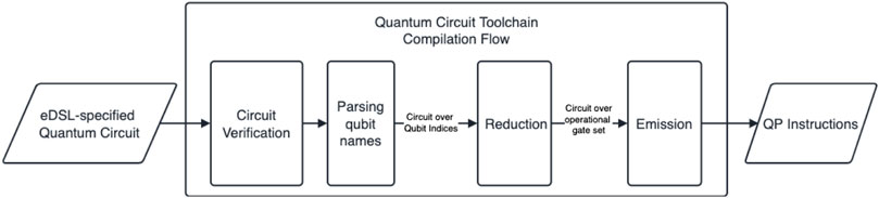
FIGURE 1. Haskell Quantum Circuit Compilation toolchain.

4.2 Simulator implementation details

HLS design tools for FPGAs (like Intel’s Quartus/Intel’s FPGA OpenCL Compiler and Xilinx’s SDAccel toolchain) have been growing in popularity and effectiveness over the past decade; making it possible to develop customized FPGA architectures for domain-specific problems in a relatively high-level language like OpenCL, without requiring knowledge of an HDL like Verilog.

The presented simulator is written in OpenCL and built using Intel/Altera SDK for OpenCL. We used Altera Offline Compiler (aoc) version 17.1. The architecture we have implemented is a baseline implementation of a full state vector-based quantum circuit simulator. The simulator is universal, with direct on board support for the H, X, Y, Z, and R_m (integer-parametrised phase gate) gates and any controlled variations of them, up to a static maximum number of controls per gate. We currently make use of the dynamic scheduling of the NDRange OpenCL construct to submit gate applications to the kernel architecture on the board. Figure 2 show the steps involved in a circuit simulation. The QP instructions generated from the compilation toolchain are read from disk on the host CPU. These instructions contain the qubit count of the circuit, and based on this sufficient memory is then allocated on the host and device. The current representation used for the state vector storage in memory is using 32-bit floating-point complex numbers, meaning we need to allocate 2ⁿ × (2 × 4) bytes to simulate the given circuit. Based on user input at runtime, the initial quantum state of the system is set and then copied to the device DRAMs.

FIGURE 2

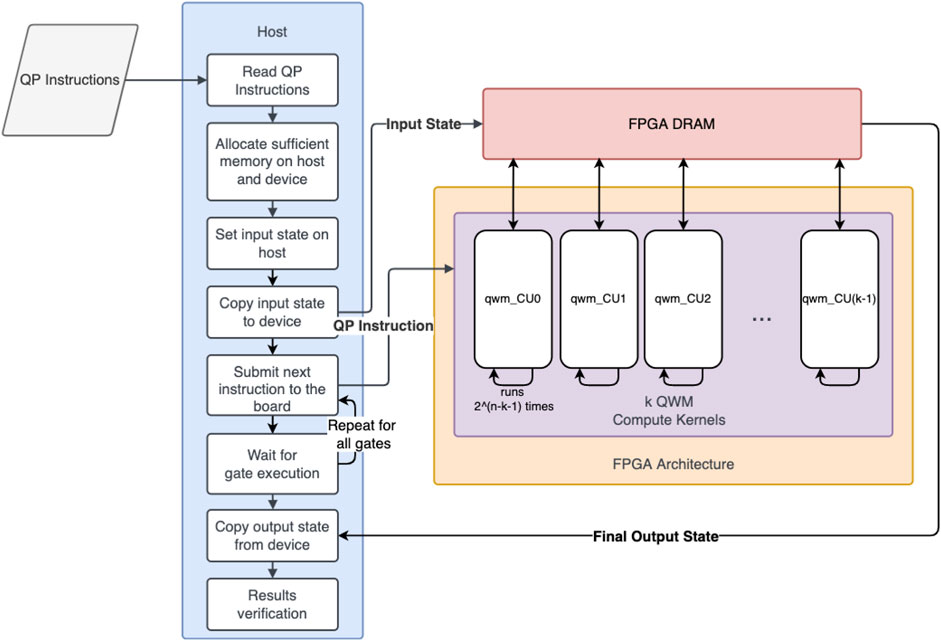
FIGURE 2. QProblem to FPGA flow for an Over-PCIe architecture. At each gate, the QP instruction is sent to the compute units over the host-FPGA PCIe connection.

Currently all FPGA architectures we have explored are parametrised by some values at compile time; primarily these are the number of compute units (NCU), which are the duplicated kernels that perform the CMACs required for the gate iteration computations, and the maximum number of controls per gate (NCONTROLS). Other more customized architectures may have more than these parameters at compile time, particularly for caching and manual memory buffering. Note that the NCONTROLS parameter determines the format of the input QP instructions; which the Haskell tool facilitates by generating QP instructions with a fixed total number of controls per gate. For non-pipelined architectures, these duplicated kernels may each include their own memory interfaces. However, for pipelined architectures (generally seen as more efficient), the compute units will generally receive their inputs over channels or pipes.

As discussed above, our focus is optimising the QWM simulation method with the full state vector being stored in memory. The main difficulty in performing a gate application in parallel arises from having an exponential memory space which has to be fully iterated through for a single gate computation (each control reduces the required accesses by half, but in general we still at least access an exponential subset of the memory space).

4.2.1 Classifying architectures

A QWM simulation architecture can be designed such that either all information required to run the circuit is accessible to the FPGA at the start of the circuit runtime process (i.e., caching the QP instructions in BRAMs/DRAM), or for the host process to interpret the QP file and enqueue each gate separately to the board. We distinguish between these different approaches and identify some intitial advantages and disadvantages to each:

An On-board QWM architecture is one where the QP instructions are stored in BRAMs/DRAM at the start of the circuit runtime process. The main advantages of this approach is that it eliminates all of the FPGA-host communication overhead, which is over a relatively slow PCIe connection, and it allows for cross-gate optimizations on board (e.g., using the same memory buffer for multiple gates). The main disadvantage is that the architecture requires extra resource overhead on the FPGA fabric to store and process the QP, and schedule gate simulations.

On the other hand, an Over-PCIe QWM architecture is one where the host process reads the QP instructions from a file and enqueues each gate to the board one-by-one. While communicating over PCIe is much slower than on-board communication via BRAMs, if loading a gate from the host can occur concurrently with computations in the kernels, then that communication time eventually becomes negligible for larger qubit counts; as the gate execution time grows exponentially with the number of qubits. This is the primary motivator for exploring the design space of simulators with this approach: at scale, the host-FPGA communication time is negligible. This architecture can be implemented with OpenCL’s NDRange construct, making use of the compiler’s automatic dynamic scheduling.

A further category along which we can divide architectures is pipelining. While most HLS compilation tools have functionality to automatically pipeline loops, the main motivator for designing an explicitly-pipelined architecture is control over the data paths of the amplitudes from memory to the compute units; allowing for experimenting with customizable caches, and memory access patterns.

We refer back to the work by Lee et al. (2016) where the authors distinguish and describe three types of architectures: concurrent, pipelined, and a novel serial-parallel architecture. The described serial-parallel architecture resembles what we describe as pipelined here (with dynamically scheduled gates and the gate executions being pipelined); with one key difference: the proposed architecture is for a quantum circuit simulation whose state vector fits entirely on the board, significantly reducing the number of qubits which can be simulated. Our architecture expands the same pipelining methods to architectures with access to DRAM banks, allowing us to simulate up to 29 qubits in 4.3 GB of memory. Another difference is their compute units (referred to as the ALU in the architecture diagrams) are customized for optimising a particular quantum circuit, the QFT; while our architectures are designed for maximum reuseability and universality.

Currently the best-performing type of architecture we have implemented is the Over-PCIe non-explicitly pipelined type. We implement this using our described NDRange approach and our results are presented based on this architecture. As we have yet to implement any caching or memory access pattern optimizations, we believe this outperforms the other designs due to the OpenCL NDRange dynamic scheduler being far more efficient for a memory access pattern as random as we currently allow than our single-task kernel approaches for on-board simulation. Since we use an NDRange kernel and no channels for explicit pipelining, our CPU and GPU comparison targets are evaluated based on the same kernel design as the FPGA. The implementation of this kernel compute unit is described in the next section.

4.2.2 Compute unit kernel details

The host initializes a queue for submitting kernel jobs to the board and is now ready to start submitting QP instructions representing quantum gates to the FPGA. The architecture’s NCU parameter defines number of identical compute units using the OpenCL num_compute_units attribute, over which the 2ⁿ⁻¹ NDRange work items are distributed, such that each kernel runs 2^n−k−1 times per gate. The host waits for the queue to finish before submitting the next gate. In its loop, the kernel knows its current gate iteration index based on its own compute unit index and the work item index passed to it by the NDRange scheduler. Based on this, it can compute the required amplitude indices for the target qubit and the current iteration, read the amplitudes directly from the DRAM, perform the gate computation, and write them back.

The compute unit kernel’s inputs at each gate are the following:

• t: gate target qubit index,

• c₀…c_{NCONTROLS−1}: control qubit indices, equal to t to specify no control

• mat₀…mat₃: gate matrix values; generated by the host after parsing the gate code from the QP file.

As an NDRange kernel, the compute unit also implicitly receives a global ID representing the current gate iteration (i): this represents this kernel’s current step in the execution of one gate. The compute unit starts by using the target qubit index and the gate iteration index to generate the indices of the pair of amplitudes required for this iteration. It generates these by finding the ith integer whose tth qubit is cleared; this is the first of the pair of indices. The second index is then found by adding the target stride (2^t) to the first index. Finding this amplitude is straightforward, has O(1) complexity, and is implementable with bit-wise logic. In particular, our implementation uses the same bit-wise logic as Kelly (2018) for their OpenCL simulator targeted at GPUs. Next, the kernel processes the controls for this iteration based on this rule: if the control value is not the target qubit, check if the amplitude indices have the bit at the control qubit’s position set to one; if so, this control’s test passes and move on to the next. Note that the number of controls which need to be processed at each gate iteration is static and defined by the NCONTROLS parameter; thus the controls processing stage is parallelisable for any gate. If all the control tests pass, then the iteration step continues with the computation: it reads the amplitudes from the DRAM, performs the gate computation (complex matrix-vector multiplication implemented with CMACs), and writes the results back to the DRAM.

After all gates are submitted to the board and finish executing, the final state is read out from the FPGA’s DRAM and written to an output file by the host. These results can then be verified.

5 The Lattice Boltzmann method

The present research effort aims to develop quantum-algorithm implementations of the Lattice Boltzmann method (LBM) for large-scale fluid dynamics simulations. As a first important step toward this, quantum algorithm for less complex Lattice Boltzmann methods, i.e. not modelling the full Navier-Stokes equations, are considered here. For context, first the Lattice Boltzmann equation forming the basis for the LBM is presented, followed by a detailed description of the reduced LB methods investigated here.

The Lattice Boltzmann equation used here is derived from a discrete-velocity discretization of the Bhatnagar-Gross-Krook (BGK) equation, such that the discretized particle distribution function is governed by the following equation:

$\frac{\partial f_a}{\partial t}+{\mathbf{e}}_a\cdot \nabla f_a=-\frac{1}{\tau }\left(f_a-f_a^{eq}\right)(4)$

with f_a(x, t) = f(x, e_a, t) is the non-equilibrium distribution for discrete velocity e_a for a ∈ [0, n_DV − 1], $f_a^{eq}$ is the corresponding equilibrium distribution function and τ represents the relaxation time. For iso-thermal LBM models, based on the two-dimensional D2Q9 model, or the three-dimensional D3Q15, D3Q19 and D3Q27 models, the equilibrium distribution function can be written as,

$f_a^{eq}=\rho w_a\left[1+\frac{3}{c^2}{\mathbf{e}}_a\cdot \mathbf{V}+\frac{9}{2c^4}{\left({\mathbf{e}}_a\cdot \mathbf{V}\right)}^2-\frac{3}{2c^2}\mathbf{V}\cdot \mathbf{V}\right]\text{\hspace{0.17em};\hspace{0.17em}}a\in \left[0,n_{DV}-1\right](5)$

where V = (u,v,w)^T is the fluid velocity vector, w_a is a weighting factor and e_a is a discrete velocity, while n_DV denotes the number of discrete velocities in the model. The lattice speed c is defined as c = δx/δt. The definition of the lattice speed c provides an explicit link between lattice spacing δx and time step δt. In the Lattice Boltzmann method (LBM), physical space is discretized using a regular lattice in a manner coherent with velocity-space discretization to preserve the conservation laws and to ensure the correct behavior of the macroscopic variables. Specifically, during a single time step, discrete values of distribution function f_a propagate in the direction of their corresponding discrete-velocity e_a to the nearest neighboring lattice point in that direction. Based on this “streaming” from on lattice point to a nearest neighbor lattice point the evolution of f_a can be written as,

$f_a\left({\mathbf{x}}_i+{\mathbf{e}}_a\delta t,t+\delta t\right)-f_a\left({\mathbf{x}}_i,t\right)=-\frac{\delta t}{\tau }\left[f_a\left({\mathbf{x}}_i,t\right)-f_a^{eq}\left({\mathbf{x}}_i,t\right)\right](6)$

The discretized distribution functions f_a and $f_a^{eq}$ are related to the fluid density and momenta as follows,

$\rho =\sum _{a=0}^{n_{DV}-1}{f}_a=\sum _{a=0}^{n_{DV}-1}{f}_a^{eq}\text{\hspace{0.17em};\hspace{0.17em}}\rho \mathbf{V}=\sum _{a=0}^{n_{DV}-1}{\mathbf{e}}_a{f}_a=\sum _{a=0}^{n_{DV}-1}{\mathbf{e}}_a{f}_a^{eq}(7)$

In Lattice Boltmann Methods, the implementation of Eq. 6 employs the stream-collide approach, i.e., the update of f_a from time t to t + δt is performed in two steps:

• Collision step. Creates an intermediate update of f_a to $f_a^{\mathit{int}}$ based on collision term:

$f_a^{\mathit{int}}\left({\mathbf{x}}_i,t\right)=f_a\left({\mathbf{x}}_i,t\right)-\frac{\delta t}{\tau }\left[f_a\left({\mathbf{x}}_i,t\right)-f_a^{eq}\left({\mathbf{x}}_i,t\right)\right](8)$

• Streaming step represents the convection on the left-hand side of Eq. 6, i.e., based on intermediate update $f_a^{\mathit{int}}$ the final update is computes as,

$f_a\left({\mathbf{x}}_i+{\mathbf{e}}_a\delta t,t+\delta t\right)=f_a^{\mathit{int}}\left({\mathbf{x}}_i,t\right)(9)$

Clearly in the LBM, the non-linearity of the Navier-Stokes equations is represented in numerical moments defining fluid velocity from the non-equilibrium distribution function f_a and the product terms involving fluid velocity and discrete velocities in the local equilibrium distribution function $f_a^{eq}$ defined in Eq. 5.

6 D1Q3 Lattice Boltzmann model

To facilitate quantum algorithm development, further reduced lattice Boltzmann models are considered. Here, the D1Q3 model is considered, as a model non-linear equation governing (some of) the nonlinear dynamics of a one-dimensional fluid flow. For the D1Q3 model, the direction vectors e_i, i ∈ [0, 2], density and velocity are defined as,

$e_i=\left\{\begin{array}{ccc}\hfill -1& \hfill \text{for}\hfill & i=0\hfill \\ \hfill 0& \hfill \text{for}\hfill & i=1\hfill \\ \hfill +1& \hfill \text{for}\hfill & i=2\hfill \end{array}\right.\text{\hspace{0.17em};\hspace{0.17em}}\rho =\sum _0^2{f}_i\text{\hspace{0.17em};\hspace{0.17em}}u=f_2-f_0(10)$

and for the collision term,

$\vec{Q}=-dt\left(\frac{\vec{f}-{\vec{f}}^{eq}}{\tau }\right)=-\frac{dt}{\tau }\left(\begin{array}{c}\hfill \frac{1}{2}\left(f_0+f_2-{\left(f_2-f_0\right)}^2-\frac{1}{3}\right)\hfill \\ \hfill \left(f_1+{\left(f_2-f_0\right)}^2-\frac{2}{3}\right)\hfill \\ \hfill \frac{1}{2}\left(f_0+f_2-{\left(f_2-f_0\right)}^2-\frac{1}{3}\right)\hfill \end{array}\right)(11)$

and therefore,

${\vec{f}}^{eq}=\left(\begin{array}{c}\hfill \frac{1}{2}\left[\frac{1}{3}-\left(f_2-f_0\right)+{\left(f_2-f_0\right)}^2\right]\hfill \\ \hfill \frac{2}{3}-{\left(f_2-f_0\right)}^2\hfill \\ \hfill \frac{1}{2}\left[\frac{1}{3}+\left(f_2-f_0\right)+{\left(f_2-f_0\right)}^2\right]\hfill \end{array}\right)=\left(\begin{array}{c}\hfill \frac{1}{2}\left[\frac{1}{3}-u+u^2\right]\hfill \\ \hfill \frac{2}{3}-u^2\hfill \\ \hfill \frac{1}{2}\left[\frac{1}{3}+u+u^2\right]\hfill \end{array}\right)(12)$

for u ≥ 0, therefore f₂ ≥ f₀. For meaningful choices of positive u, all three components $f_0^{eq}$, $f_1^{eq}$ and $f_2^{eq}$ will be positive numbers. Since the Lattice Boltzmann Method was derived under the assumption that $\vec{f}$ will be a relatively small deviation from ${\vec{f}}^{eq}$, we can therefore also assume that f₀, f₁ and f₂ will be positive numbers for meaningful choices of positive u.

7 Modified D1Q3 Lattice Boltzmann Method

To facilitate the implementation using the quantum circuit model, a number of modifications and re-normalizations are introduced in this section. Firstly, the original 3 direction vectors are replaced by 4, where the original single “rest” velocity is replaced by two identical ‘rest’ velocities. This results in the following directions vectors, with corresponding definitions of density and velocity,

$e_i=\left\{\begin{array}{ccc}\hfill -1& \hfill \text{for}\hfill & i=0\hfill \\ \hfill 0& \hfill \text{for}\hfill & i=1\hfill \\ \hfill 0& \hfill \text{for}\hfill & i=2\hfill \\ \hfill +1& \hfill \text{for}\hfill & i=3\hfill \end{array}\right.\text{\hspace{0.17em};\hspace{0.17em}}\rho =\sum _0^3{f}_i\text{\hspace{0.17em};\hspace{0.17em}}u=f_3-f_0(13)$

The original f₁ distribution function will be replaced by two identical distributions functions f₁ and f₂ in the modified model. Then, the corresponding equilibrium distribution functions become,

${\vec{f}}^{eq}=\left(\begin{array}{c}\hfill \frac{1}{2}\left[\frac{1}{3}-\left(f_2-f_0\right)+{\left(f_2-f_0\right)}^2\right]\hfill \\ \hfill \frac{1}{2}\left[\frac{2}{3}-{\left(f_2-f_0\right)}^2\right]\hfill \\ \hfill \frac{1}{2}\left[\frac{2}{3}-{\left(f_2-f_0\right)}^2\right]\hfill \\ \hfill \frac{1}{2}\left[\frac{1}{3}+\left(f_2-f_0\right)+{\left(f_2-f_0\right)}^2\right]\hfill \end{array}\right)=\left(\begin{array}{c}\hfill \frac{1}{2}\left[\frac{1}{3}-u+u^2\right]\hfill \\ \hfill \frac{1}{2}\left[\frac{2}{3}-u^2\right]\hfill \\ \hfill \frac{1}{2}\left[\frac{2}{3}-u^2\right]\hfill \\ \hfill \frac{1}{2}\left[\frac{1}{3}+u+u^2\right]\hfill \end{array}\right)(14)$

For the flow field at rest (u = 0), the distributions functions are therefore,

${\vec{f}}^{eq}=\vec{f}={\left[\frac{1}{6};\frac{1}{3};\frac{1}{3};\frac{1}{6}\right]}^T(15)$

To next modification step aims to remove the “constant” factors 1/3 and 1/6, by introduction a re-scaled distribution function $\vec{g}$ defined as the deviation away from the “rest” state defined in Eq. 15 as,

$\vec{g}=\vec{f}-\left(\begin{array}{c}\hfill \frac{1}{6}\hfill \\ \hfill \frac{1}{3}\hfill \\ \hfill \frac{1}{3}\hfill \\ \hfill \frac{1}{6}\hfill \end{array}\right)\text{\hspace{0.17em};\hspace{0.17em}}{\vec{g}}^{eq}={\vec{f}}^{eq}-\left(\begin{array}{c}\hfill \frac{1}{6}\hfill \\ \hfill \frac{1}{3}\hfill \\ \hfill \frac{1}{3}\hfill \\ \hfill \frac{1}{6}\hfill \end{array}\right)=\left(\begin{array}{c}\hfill -\frac{u}{2}+\frac{u^2}{2}\hfill \\ \hfill -\frac{u^2}{2}\hfill \\ \hfill -\frac{u^2}{2}\hfill \\ \hfill \frac{u}{2}+\frac{u^2}{2}\hfill \end{array}\right)(16)$

Alternatively, ${\vec{g}}^{eq}$ can be written as,

${\vec{g}}^{eq}=\left(\begin{array}{c}\hfill \frac{1}{2}\left[-\left(g_3-g_0\right)+{\left(g_3-g_0\right)}^2\right]\hfill \\ \hfill -\frac{1}{2}{\left(g_3-g_0\right)}^2\hfill \\ \hfill -\frac{1}{2}{\left(g_3-g_0\right)}^2\hfill \\ \hfill \frac{1}{2}\left[+\left(g_3-g_0\right)+{\left(g_3-g_0\right)}^2\right]\hfill \end{array}\right)(17)$

For this re-scaled D1Q3 model, the density and velocity are now defined as,

$\rho =1+\sum _0^3{g}_i\text{\hspace{0.17em}\hspace{0.17em};\hspace{0.17em}\hspace{0.17em}\hspace{0.17em}}u=g_3-g_0(18)$

7.1 Biased quantum floating point representation

In the current implementation of the D1Q3 model, the idea is to represent the (scaled) distribution function values g_i, i ∈ [0, 3] and u/c) with a specialized (biased) quantum floating-point format. The motivation for choosing this format is the wider range of numbers that can be represented than in a fixed-point representation for the same number of qubits used. To minimize quantum-circuit width, a reduced number of mantissa and exponent bits is used as compared to IEEE-754 single-precision format. However, for the considered problems a scaling was used so that the ranges of numbers to be represented is both limited and predictable. For the D1Q3 model, where the numbers will be ≪ 1, this choice of parameters is further detailed later this section.

The quantum floating-point representation used here builds on earlier work by Steijl (2022) and involves reduced-bit representations of exponent and mantissa relative to single-precision in the IEEE-754 standard to facilitate quantum circuit implementations on current and near-future quantum hardware with relatively small number of qubits $(<100)$. A key feature of the used quantum floating-point representation is that following the IEEE-754 standard, it employs sub-normal numbers and consistent rounding (here, rounding-down to nearest). The number of mantissa qubits is defined by N_M, where only N_M − 1 mantissa qubits are stored following the “hidden-qubit” approach from IEEE-754. Then, the number of qubits storing the exponent is defined by N_E. In the present work, N_E = 3, and exponent 0 (exponent qubits in state $\left|000\right.⟩$) represent sub-normal numbers and zero as in the IEEE-754 standard. The maximum value for exponent is 7 (exponent qubits in state $\left|111\right.⟩$) refers to “overflow” conditions, as used in the IEEE-754 standard. For N_E = 3, an “unbiased” exponent formulation would be equivalent to an exponent bias of 3. To optimize for the small numbers occurring in considered problems, a bias toward smaller numbers is used here. Clearly, the choice of N_M is crucial in achieving the required accuracy. For equilibrium distribution functions, terms linear and quadratic in u/c are combined, and N_M = 3 was found to lead to excessive rounding or truncation for most values of u/c. Clearly, N_M ≥ 4 should be used. However, since the lattice-based models considered here represent conservation of mass, momentum and energy in the fluid, rounding of numbers will have a significant effect on accuracy, particularly in multiple time-step simulations. Therefore, realistically it can be expected that N_M ∈ (Fillion-Gourdeau and Lorin, 2019; Bonny and Haq, 2020) is needed for realistic engineering applications. In this work, circuits for N_M = 4 are shown as illustration, and the complexity analysis shown in Section 10 addresses in detail how the circuit width increases with N_M.

Following IEEE-754, signed floating-point numbers are stored as “$\left|\mathrm{sign}|\text{exponent}|\text{mantissa}\right.⟩$,” while the sign qubit is omitted where unsigned numbers are used in the quantum-circuit implementation. For “signed” additions or subtractions of two numbers, two (N_M + 1)-qubit registers as input to a modulo adder are created as follows. First, the hidden qubits are added to the mantissa, followed by re-normalization (to account for possible difference in exponent) to create two (N_M + 1)-qubit inputs with $\left|0\right.⟩$ as most-significant qubit. Where required a conversion to 2’s complement is performed, so that negative numbers have the most-significant qubit in state $\left|1\right.⟩$. After addition/subtraction, the outcome is converted back to the quantum floating-point format, where a sign-qubit defines the sign and with mantissa no longer in 2’s complement, i.e., back into (N_M − 1)-qubit “hidden-qubit” representation.

For N_M = 4 and N_E = 3, the sub-normal numbers with the corresponding “negative” (N_M + 1)-qubit mantissa representation using 2’s complement method are shown in Table 1 for “bias = 3” and “bias = 8.” Here, “bias = 3” corresponds to the “standard” floating-point format with a symmetric bias. As can be seen from Table 1, with symmetric bias (“bias = 3”), terms involving u² (O(10^–2) will always be sub-normal and often truncated to 0. For “bias = 8,” it can expected that u² can be represented either as non-zero sub-normal or normalized numbers.

TABLE 1

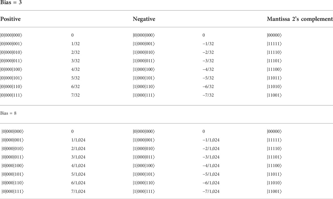
TABLE 1. Sub-normal numbers for N_M = 4 and N_E = 3. Leading qubit acts as “sign” qubit. In 2’s complement “hidden qubit” is represented.

For N_M = 4 and N_E = 3, the normalized numbers for $\left|e2|e1|e0\right.⟩=\left|110\right.⟩$ with the corresponding “negative” using 2’s complement method are shown in Table 2 for “bias = 3” and “bias = 8.”

TABLE 2

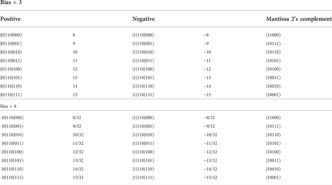
TABLE 2. Example normalized numbers for N_M = 4 and N_E = 3. Leading qubit acts as “sign” qubit. In 2’s complement “hidden qubit” is represented.

For the maximum exponent $(\left|e2|e1|e0\right.⟩=\left|110\right.⟩)$, the values for “bias = 8” shown in Table 2 indicate that despite the greatly reduced value of the maximum number that can be represented relative to the symmetric bias case (“bias = 3”), the components of distribution function $\vec{g}$ and velocity u/c will be so small that these can still be represented without risking an overflow, as discussed next.

The choice of suitable values for N_E and exponent bias for the scaled and normalized D1Q3 model can be made based on the flow physics that is modelled. For the D1Q3 model, the lattice speed of sound is defined as $c_s=c/\sqrt{3}$. The iso-thermal model used here was derived for flows with weak or negligible compressibility effects. For a compressible fluid, a local Mach number can be defined as: $M=|u|/c_s=\sqrt{3}|u|/c$. For the weakly compressible-flow conditions it is required that M < 0.3 or smaller. Therefore, u/c should generally be limited to maximum values of 0.1–0.15. Clearly, in the modified and re-scaled D1Q3 model employing a symmetric bias will introduce a range of numbers far from optimal for the D1Q3 model. As shown in Table 2, for N_E = 3, a bias of 8 gives ample margin at the upper end of the floating-point range when representing u/c. However, since the (scaled) and re-normalized equilibrium distribution functions combine terms O(u) and O(u²) it was decided that a bias of 9 could potentially leave too little margin in the floating-point representation of g_i components.

7.2 Quantum circuit implementation—Streaming operation

In Lattice Boltzmann models, the non-linear convection term of the Navier-Stokes equation is effectively (partly) replaced by a linear streaming of the distribution functions from one lattice point to a neighboring lattice point during a time step. For the modified D1Q3 model, only two directions specified by $\left|dv1|dv0\right.⟩=\left|00\right.⟩$ (“−1”) and $\left|dv1|dv0\right.⟩=\left|11\right.⟩$ (“+1”) need to be considered since the remaining two are “at rest.” Assuming a uniformly-spaced one-dimensional domain with 64 lattice points and periodic boundary conditions, a possible quantum-circuit implementation for the streaming operations is illustrated in Figure 3. This type of linear operators was previously detailed by Todorova and Steijl (2020) and will therefore not be analyzed further here.

FIGURE 3

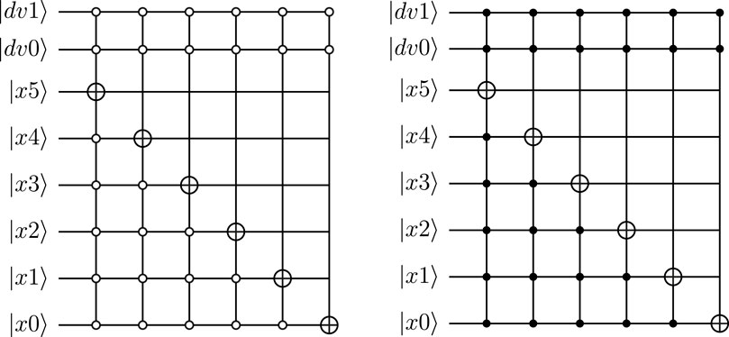
FIGURE 3. Quantum circuit implementing the “streaming” operation for directions 0 $(\left|dv1|dv0\right.⟩=\left|00\right.⟩)$ and 3 $(\left|dv1|dv0\right.⟩=\left|11\right.⟩)$ on uniformly-space 1D mesh (64 cells encoded with 6 qubits) with periodic boundary conditions. Design assumed amplitude-based encoding of data. Most-significant qubit as used in data ordering is at the top of circuits.

8 Quantum circuit implementation—Equilibrium distribution function

8.1 Mapping of computational problem on qubit register

The quantum-circuit was designed with input data encoded in qubits at the top of the circuit (most significant qubits), followed by qubits representing the output of the computation performed. The remaining qubits further “down” (i.e., less significant in the employed memory indexing) generally act as ancillae qubits or as workspace. These ancillae and workspace qubits are all initialized in state $\left|0\right.⟩$ and will be returned to $\left|0\right.⟩$ at the time of completion of the quantum circuit. In later sections, a modified and transformed design will be considered were the ordering is altered to facilitate efficient simulation. For the original circuit, the qubit register for N_M = 4 and N_E = 3 can be summarized as follows:

$\begin{array}{cc}\hfill \left|dv1|dv0\right.⟩& \text{indices\hspace{0.17em}for\hspace{0.17em}}4\text{\hspace{0.17em}discrete\hspace{0.17em}velocities}\hfill \\ \hfill \left|eu2|eu1|eu0\right.⟩& 3-\text{bit\hspace{0.17em}representation\hspace{0.17em}of\hspace{0.17em}exponent\hspace{0.17em}of\hspace{0.17em}}u\hfill \\ \hfill \left|su\right.⟩& \text{sign\hspace{0.17em}bit\hspace{0.17em}of\hspace{0.17em}input\hspace{0.17em}velocity\hspace{0.17em}}u\hfill \\ \hfill \left|mu2|mu1|mu0\right.⟩& 3-\text{bit\hspace{0.17em}representation\hspace{0.17em}of\hspace{0.17em}mantissa\hspace{0.17em}of\hspace{0.17em}}u\hfill \\ \hfill \left|eg2|eg1|eg0\right.⟩& 3-\text{bit\hspace{0.17em}representation\hspace{0.17em}of\hspace{0.17em}exponent\hspace{0.17em}of\hspace{0.17em}}{g}^{eq}\hfill \\ \hfill \left|sg\right.⟩& \text{sign\hspace{0.17em}bit\hspace{0.17em}of\hspace{0.17em}output\hspace{0.17em}}{g}^{eq}\hfill \\ \hfill \left|mg2|mg1|mg0\right.⟩& 3-\text{bit\hspace{0.17em}representation\hspace{0.17em}of\hspace{0.17em}mantissa\hspace{0.17em}of\hspace{0.17em}}{g}^{eq}\hfill \\ \hfill \left|esq2|esq1|esq0\right.⟩& 3-\text{bit\hspace{0.17em}representation\hspace{0.17em}of\hspace{0.17em}exponent\hspace{0.17em}of\hspace{0.17em}}{u}^2\hfill \\ \hfill \left|msq2|msq1|msq0\right.⟩& 3-\text{bit\hspace{0.17em}representation\hspace{0.17em}of\hspace{0.17em}mantissa\hspace{0.17em}of\hspace{0.17em}}{u}^2\hfill \\ \hfill \left|cut\right.⟩& \text{state\hspace{0.17em}}\left|1\right.⟩\text{\hspace{0.17em}defines\hspace{0.17em}that\hspace{0.17em}}{u}^2\text{is\hspace{0.17em}truncated\hspace{0.17em}to\hspace{0.17em}0}\hfill \\ \hfill \left|r4|qu3|r3|qu2|r2|qu1|r1|qu0\right.⟩& \text{workspace\hspace{0.17em}qubits\hspace{0.17em}ordered\hspace{0.17em}for\hspace{0.17em}}4-\text{qubit\hspace{0.17em}addition}\hfill \\ \hfill \left|c\right.⟩& \text{workspace\hspace{0.17em}qubit\hspace{0.17em}named\hspace{0.17em}to\hspace{0.17em}represent\hspace{0.17em}’carry’\hspace{0.17em}bit\hspace{0.17em}in\hspace{0.17em}}4-\text{qubit\hspace{0.17em}addition}\hfill \\ \hfill \left|r7|r6|r5\right.⟩& \text{workspace\hspace{0.17em}qubits\hspace{0.17em}ordered\hspace{0.17em}for\hspace{0.17em}}4-\text{qubit\hspace{0.17em}squaring}\hfill \\ \hfill \left|anc\right.⟩& \text{workspace\hspace{0.17em}qubit\hspace{0.17em}}-\text{\hspace{0.17em}mostly\hspace{0.17em}used\hspace{0.17em}as\hspace{0.17em}control\hspace{0.17em}qubit}\hfill \end{array}$

This shows that 37 qubits are required in this original design. Data related to g₀ and g₃ are stored in the vector for $\left|dv1|dv0\right.⟩=\left|00\right.⟩$ and $\left|dv1|dv0\right.⟩=\left|11\right.⟩$. Similarly, states with $\left|dv1|dv0\right.⟩=\left|01\right.⟩$ and $\left|dv1|dv0\right.⟩=\left|10\right.⟩$ represent data for the (identical) distribution functions g₁ and g₂. For the floating-point representations of input u and each component of output ${\vec{g}}^{eq}$, 7 qubits are needed using the hidden-qubit approach. For the temporary storage of u², the sign bit can be omitted. In the following, for N_M = 4 and N_E = 3 an exponent “bias = 8” is used in the floating-point representations.

8.2 Overview of quantum circuit design

Figure 4 shows the first part of the quantum circuit designed to compute the equilibrium distribution function ${\vec{g}}^{eq}$ for N_M = 4 and N_E = 3. The first step involves setting $\left|icut\right.⟩=\left|1\right.⟩$ for the cases with a guaranteed truncation of u²—for N_M = 4 and N_E = 3 this truncation always occurs for $\left|eu2|eu1|eu0\right.⟩=\left|000\right.⟩$, $\left|001\right.⟩$ and $\left|010\right.⟩$. In the next step, the mantissa of u is set into the required positions in the workspace, defined by $\left|qu3|qu2|qu1|qu0\right.⟩$, for all cases without truncation of u² to 0. The operation SQ4 then computes the square of the mantissa and stores the results in $\left|r7|r6|\dots |r0\right.⟩$. Operation CC_u2 then creates a (temporary) “copy” of the u² defined in the quantum-floating format in the qubits $\left|esq2|esq1|esq0\right.⟩$ (defining exponent) and $\left|msq2|msq1|msq0\right.⟩$ (defining mantissa using hidden-qubit approach). For u² no sign qubit is needed. To clear the workspace for further use, operation ISQ4 un-computes the mantissa squaring, followed by the removal of the copy of the mantissa of u from qubits $\left|qu3|qu2|qu1|qu0\right.⟩$.

FIGURE 4

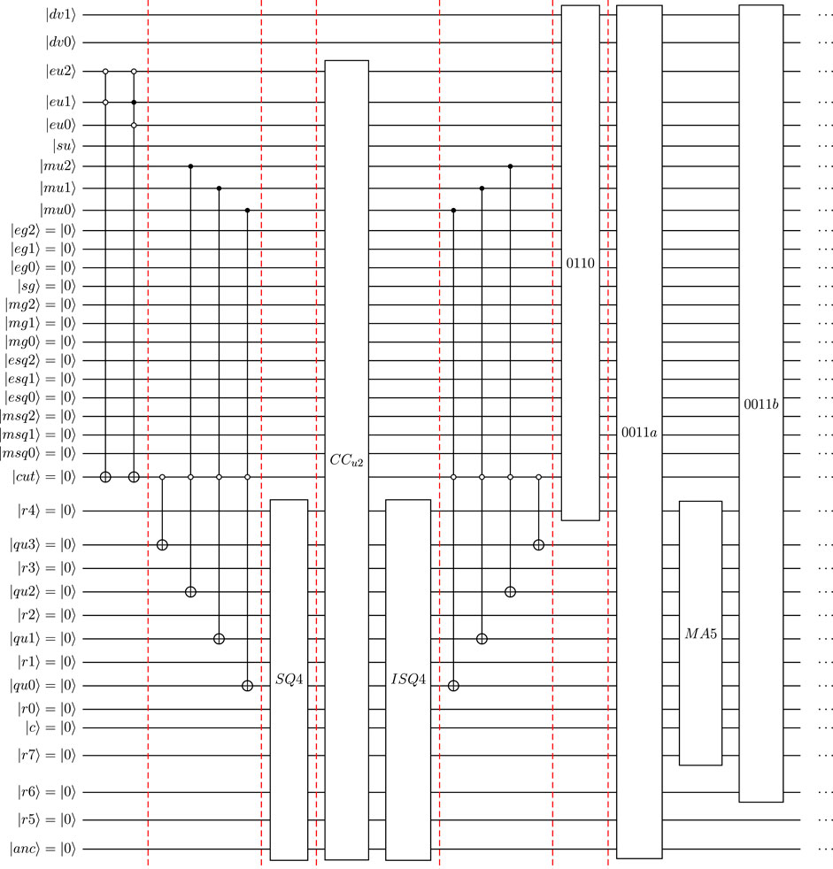
FIGURE 4. Quantum circuit design for evaluation of ${\vec{g}}^{eq}$ in modified D1Q3 model. Velocity u and distribution functions defined as quantum floating-point numbers with N_M = 4 and N_E = 3. Most-significant qubits at top of circuit. Part 1.

The quantum-circuit implementation for SQ4 and ISQ4 are shown in Figures 5, 6, respectively. Here, FAdd represents a 4-qubit Cuccaro full adder, and Rmv the un-computation of this adder. The required shift in the used shift-and-add approach are performed by Sh (in SQ4) and Sh’ (shift in reversed direction in ISQ4). Following the definition of u² in quantum floating-point format, the equilibrium distribution for directions e₁ and e₂ (defined by $\left|dv1|dv0\right.⟩=\left|01\right.⟩$ and $\left|dv1|dv0\right.⟩=\left|10\right.⟩$) is defined using the operator 0110 in Figure 4.

FIGURE 5

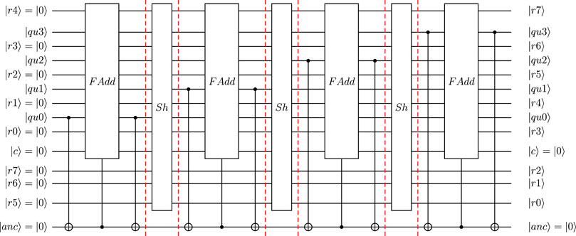
FIGURE 5. Quantum circuit defining SQ4 with 4-qubit mantissa qubits (N_M = 4, using hidden qubit approach) and a 3-qubit exponent (N_E = 3).

FIGURE 6

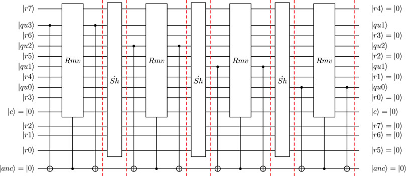
FIGURE 6. Quantum circuit defining ISQ4 with 4-qubit mantissa qubits (N_M = 4, using hidden qubit approach) and a 3-qubit exponent (N_E = 3).

To define the equilibrium distribution functions for directions e₀ and e₃ (defined by $\left|dv1|dv0\right.⟩=\left|00\right.⟩$ and $\left|dv1|dv0\right.⟩=\left|11\right.⟩$), the addition of ± u and u² is required. This addition operator for the signed values defined in the N_M = 4 and N_E = 3 format is performed using a modulo-5 Cuccaro adder, denoted by MA5. Operation 0011a initializes this addition step, followed by the operation 0011b that uses the created result to define the equilibrium distribution functions for directions e₀ and e₃ in qubits $\left|eg2|eg1|eg0\right.⟩$ (exponent), $\left|sg\right.⟩$ (sign qubit) and $\left|mg2|mg1|mg0\right.⟩$ (mantissa qubits using hidden-qubit approach).

Figure 7 shows the second part of the quantum circuit designed to compute the equilibrium distribution function ${\vec{g}}^{eq}$ for N_M = 4 and N_E = 3. The first step involves the un-computation of the modulo-5 addition (denoted by UMA5), followed by operation 0011c used to clear the inputs to this addition. Upon completion of operation 0011c, the 14 workspace qubits are all in state $\left|0\right.⟩$. However, at this stage, the temporary copy of u² still resides in qubits $\left|esq2|esq1|esq0\right.⟩$ and $\left|msq2|msq1|msq0\right.⟩$. To clear these qubits to state $\left|0\right.⟩$, the square of the mantissa of u² needs to be re-computed using SQ4. Then, CC_u2 is used to set the 6 qubits defining u² in quantum floating point format to $\left|0\right.⟩$. Then, ISQ4 un-computes the mantissa squaring step. Finally the remaining workspace qubits can be cleared along with the qubit $\left|cut\right.⟩$, which for cases with truncation of u² to 0 is re-set to $\left|0\right.⟩$.

FIGURE 7

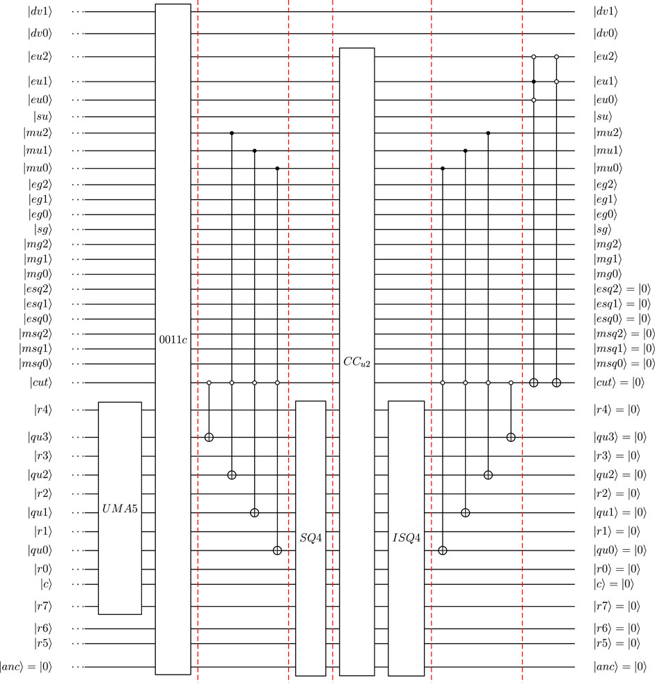
FIGURE 7. Quantum circuit design for evaluation of ${\vec{g}}^{eq}$ in modified D1Q3 model. Velocity u and distribution functions defined as quantum floating-point numbers with N_M = 4 and N_E = 3. Most-significant qubits at top of circuit. Part 2.

At this stage, the output of the quantum circuit has the required format: the qubits $\left|eg2|eg1|eg0\right.⟩$ (exponent), $\left|sg\right.⟩$ (sign qubit) and $\left|mg2|mg1|mg0\right.⟩$ define the equilibrium distribution function for all four directions in the modified D1Q3 model, while the rest of the qubits is left unchanged.

In operator 0110, the previously computed term u² is used to set −u²/2 for the two “rest” directions ($\left|dv1|dv0\right.⟩=\left|01\right.⟩$ and $\left|dv1|dv0\right.⟩=\left|10\right.⟩$). For these directions the “−” sign can be trivially introduced by setting the sign qubit of ${\left|g\right.⟩}^{eq}$, $\left|sg\right.⟩=\left|1\right.⟩$. For the direction 0 defined by $\left|dv1|dv0\right.⟩=\left|00\right.⟩$, the equilibrium distribution function is of the form −u/2 + u²/2. For this direction (and for direction 3 with distribution function of the form u/2 + u²/2), first the terms −u + u² and +u + u² are computed using a 5-qubit modulo adder MA5 (and its reverse UMA5), while the division by 2 is introduced when setting the result in quantum-floating point format. The sign change to ′ − u′ for direction 0 is created by switching to 2’s complement notation or the 4 mantissa qubits. Based on the assumption of positive input velocity u, the 5 input qubits (as “a” input to Cuccaro modulo adder) representing mantissa of u are initially set as $\left|0|mu3|mu2|mu1|mu0\right.⟩$ (with $\left|mu3\right.⟩=\left|0\right.⟩$ for sub-normal numbers). The quantum-circuit implementation of operator SgnA5 performing this sign change is shown in Figure 8. With u ≪ 1 in the D1Q3 model, the term −u + u² will always be a negative number. Since the 4 mantissa qubits of ${\vec{g}}^{eq}$ are not stored in 2’s complement formulation for negative values (i.e., the sign is defined by $\left|sg\right.⟩$), a similar sign change to SgnA5 needs to be applied on the output of the 5-qubit modulo adder. With the guaranteed negative result for direction 0, it is sufficient to perform the 2’s complement conversion on only to the 4 qubits (for N_M = 4 considered here) used to define mantissa qubits of ${\vec{g}}^{eq}$. The operator SgnB4 performs this change. Its quantum-circuit implementation is also shown in Figure 8.

FIGURE 8

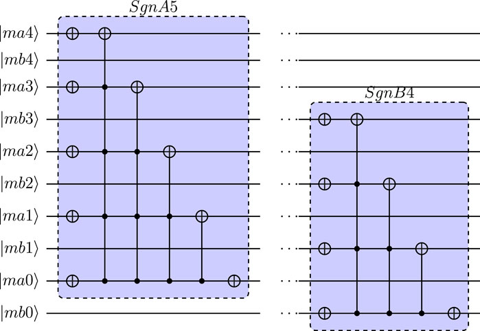
FIGURE 8. Quantum circuit-implementations of SgnA5 and SgnB4 used to introduced sign change in 5-qubit modulo addition.

9 Reduction for FPGA acceleration of QC simulation

The quantum-circuit implementation for the computation of the equilibrium distribution functions of the modified D1Q3 model shown in Figures 4, 7 will be transformed in this section to facilitate a more efficient quantum circuit simulation using FPGA acceleration. The “original” circuit designed for N_M = 4 and N_E = 3 uses 37 qubits. As a first step toward “reduced” circuits, circuit re-ordering and partial specialization of one or more qubits is used.

The key ideas behind the considered reduction/transformation are as follows:

• The circuit evaluates the distribution functions for 4 directions based on a single input u defined in quantum floating-point format—therefore specialized circuits can be created based on the selected input for u;

• The specialized input is defined using 7 qubits: $\left|eu2|ue1|e0\right.⟩$ (exponent), $\left|su\right.⟩$ (sign) and $\left|mu2|mu1|mu0\right.⟩$ (defines mantissa using hidden-qubit appraoch)—so reduced circuits with 7 fewer can be created for particular values of u;

• The two most significant qubits in the design shown in Figures 4, 7, i.e., $\left|dv1|dv0\right.⟩$ define the direction vector (i ∈ [0, 3]). If required, a further reduction or transformation can be performed, so that only the equilibrium distribution function for a single direction is evaluated. This allows a further reduction by 2 qubits relative to the original circuit;

• The qubit $\left|cut\right.⟩$ only depends on the exponent of u, so at compile time for specialized circuits this information regarding truncation of u² is known. Therefore, also $\left|cut\right.⟩$ can be eliminated in transformed circuits, specialized for specific u input

Using the above transformation steps, reduced circuits with 27 qubits can be created for N_M = 4 and N_E = 3, as compared to the original number of 37.

9.1 Further reduction

The transformation steps detailed in the previous section enabled a reduction to computational kernels with 27 qubits as compared to the 37-qubit full circuit. For a further reduction, the 14-qubit workspace needs to be transformed. Specifically, the arithmetic operations in SQ4, ISQ4, MA5 and UMA5 need to be transformed and specialized for specific inputs. Since the Quantum Computer simulator used here employs a memory allocation with the top qubits in the circuits shown acting as the most significant qubits, the overall circuit design shown in Figures 4, 7 needs to be changed: the qubits defining workspace need to be moved towards the top of the quantum circuit, and therefore, the qubits storing u² and ${\vec{g}}^{eq}$ in quantum floating-point format need to be moved down toward less significant bit locations.

Following this re-ordering, a further reduction requires specializing (and factoring out) one or more mantissa qubits, starting from the most significant mantissa qubit of u, i.e., $\left|qu3\right.⟩$, followed by $\left|mu2\right.⟩$, etc. Using this approach, requires transformation to the u² computations as well as modulo-additions, as discussed in following sections.

9.2 Reduction of the u² computation

To illustrate the further reduction of the number of qubits, the computation of u² is analyzed first. In the interest of clarity, this section will consider the reduced circuits for the evaluation of $g_1^{eq}(\left|dv1|dv0\right.⟩=\left|01\right.⟩)$ and $g_2^{eq}(\left|dv1|dv0\right.⟩=\left|10\right.⟩)$, since these identical terms only involve the term u²/2. Figure 9 shows the reduced quantum circuit with 26 qubit resulting from eliminating the two most-significant mantissa qubits in squaring operations for N_M = 4 and N_E = 3. As can be seen, the circuit only involves the two mantissa qubits $\left|qu1|qu0\right.⟩$, and SQ4 and ISQ4 represent reduced squaring (and un-computation) for specific choices of $\left|qu3|qu2\right.⟩$. For the further reduction by 2 qubits to 26-qubits, the operations SQ4 and ISQ4 involve 12 qubits in the workspace. The operation CC_u2 sets the squared-velocity values in terms of quantum-floating point format in $\left|esq2|esq1|esq0\right.⟩$ (exponent) and $\left|msq2|msq1|msq0\right.⟩$ (mantissa), and for the considered reduction to 26 qubits, the quantum circuit implementations for CC_u2 are detailed for $\left|eu2|eu1|eu0\right.⟩=\left|011\right.⟩$, $\left|100\right.⟩$ or $\left|101\right.⟩$ in Figure 10. For $\left|eu2|eu1|eu0\right.⟩=\left|110\right.⟩$, the operator is identical to that for $\left|101\right.⟩$, apart from the NOT operation on $\left|esq1\right.⟩$ that for $\left|eu2|eu1|eu0\right.⟩=\left|110\right.⟩$ is performed on $\left|esq2\right.⟩$ instead. Figure 11 shows the quantum-circuit definitions of the reduced mantissa-squaring and adders (as well as the reverse circuits), for the 26-qubit reduced quantum-circuit implementation.

FIGURE 9

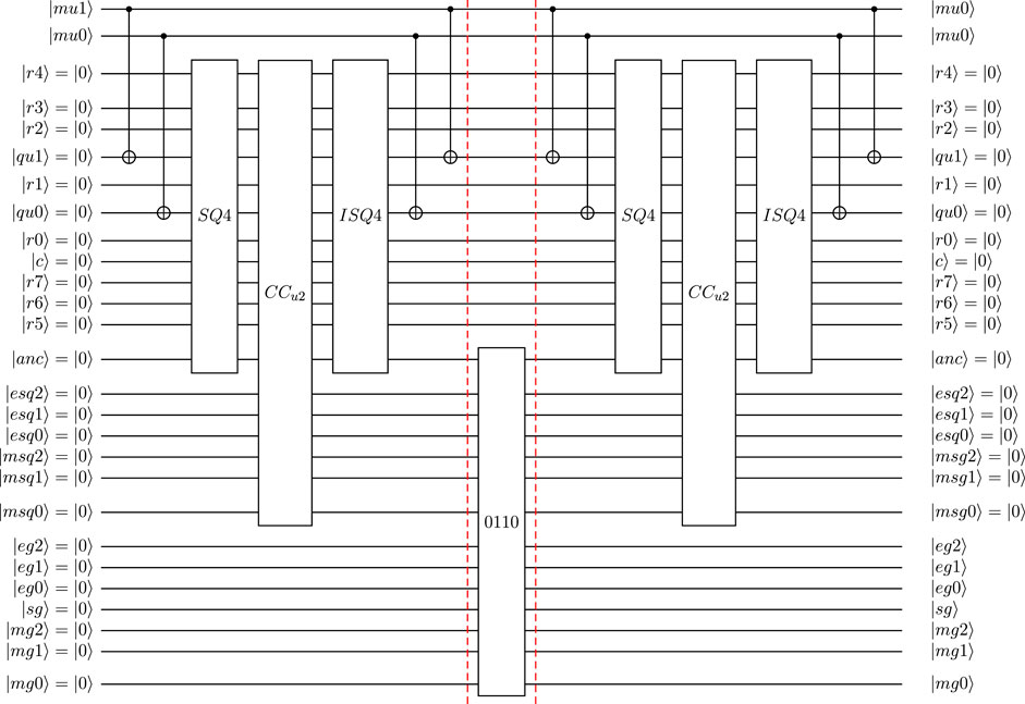
FIGURE 9. Reduced circuit with 26 qubits: $\left|dv1|dv0\right.⟩=\left|01\right.⟩$ or $\left|10\right.⟩$, $\left|eu2|eu1|eu0\right.⟩=\left|011\right.⟩$, $\left|100\right.⟩$, $\left|101\right.⟩$ or $\left|110\right.⟩$ (and therefore $\left|cut\right.⟩=\left|0\right.⟩$).

FIGURE 10

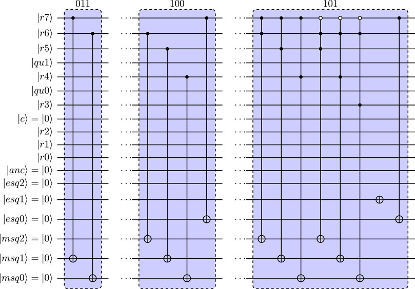
FIGURE 10. CC_u2 for reduced circuit with 26 qubits. Squared velocity u² defined as quantum floating-point numbers with N_M = 4 and N_E = 3. Label indicates for which $\left|eu2|eu1|eu0\right.⟩$ circuit was derived.

FIGURE 11

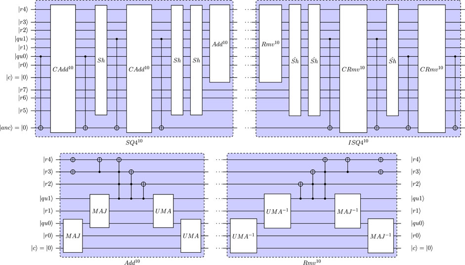
FIGURE 11. Definition of SQ4 and ISQ4 for reduced quantum circuit (26 qubit) for |mu2)= |0)= (|qu3|qu2)= |10) for normalized input). CAdd¹⁰ and CRmv¹⁰ are defined as Add¹⁰ and Rmv¹⁰ with |anc) acting as control qubit.

Figure 12 shows the reduced quantum circuit with 25 qubit resulting from eliminating the three most-significant mantissa qubits in squaring operations for N_M = 4 and N_E = 3. As can be seen, the circuit only involves the mantissa qubit $\left|qu0\right.⟩$, and SQ4 and ISQ4 represent reduced squaring (and un-computation) for specific choices of $\left|qu3|qu2|qu1\right.⟩$. For the further reduction by 3 qubits to 25-qubits, the operations SQ4 and ISQ4 involve 11 qubits in the workspace as can be seen in the quantum-circuit implementations shown in Figure 13. For the reduced quantum circuit with 25 qubits, Figure 14 shows the quantum-circuit implementation of the “shift” operations used in the “shift-and-add” approach. For N_M = 4, a further reduction to 24 qubis can be made, by reducing out qubit $\left|qu0\right.⟩$ from the SQ4 and ISQ4 operations. For this further reduction to 24 qubits, quantum-circuit implementation of operations SQ4 and ISQ4 are shown in Figure 15. The addition and remove operators are specialized for the 4 mantissa qubits $\left|qu3|qu2|qu1|qu0\right.⟩=\left|1001\right.⟩$.

FIGURE 12

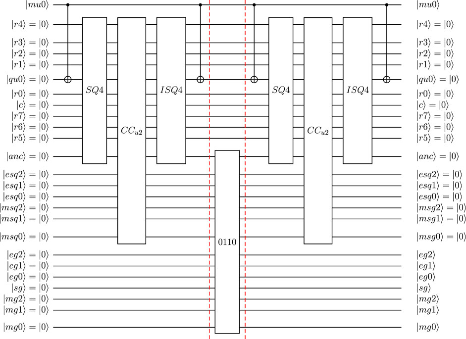
FIGURE 12. Reduced circuit with 25 qubits: $\left|dv1|dv0\right.⟩=\left|01\right.⟩$ or $\left|10\right.⟩$, $\left|eu2|eu1|eu0\right.⟩=\left|011\right.⟩$, $\left|100\right.⟩$, $\left|101\right.⟩$ or $\left|110\right.⟩$ (and therefore $\left|cut\right.⟩=\left|0\right.⟩$).

FIGURE 13

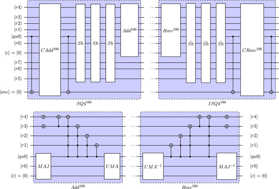
FIGURE 13. Definition of SQ4 and ISQ4 for reduced quantum circuit (25 qubit) for |mu2|mu1〉 = |00〉 = (|qu3|qu2|qu1〉 = |100〉 for normalized input). CAdd¹⁰⁰ and CRmv¹⁰⁰ are defined as Add¹⁰⁰ and Rmv¹⁰⁰ with |anc〉 acting as control qubit.

FIGURE 14

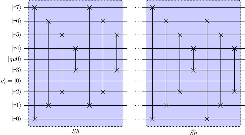
FIGURE 14. Shift operators used for left- and right-shifting of results register in reduced circuit with 25 qubits.

FIGURE 15

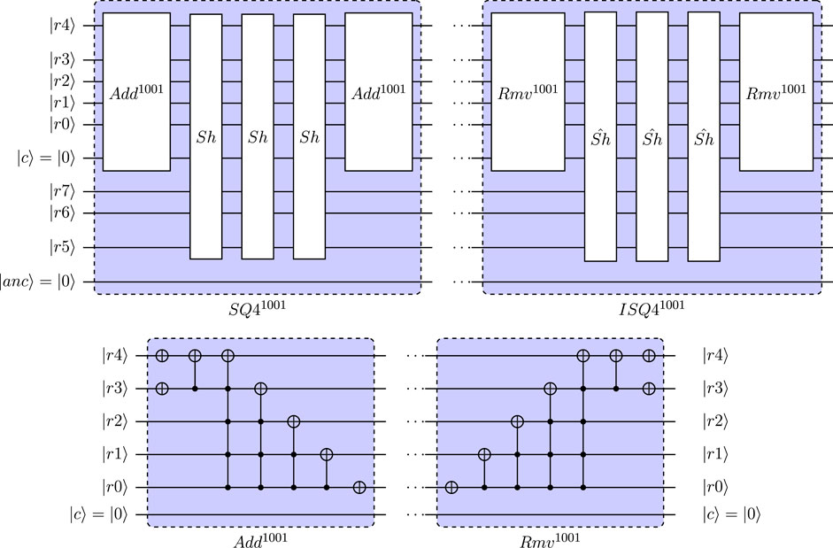
FIGURE 15. Definition of SQ4 and ISQ4 for reduced quantum circuit (24 qubit) for $\left|mu2|mu1|mu0\right.⟩=\left|001\right.⟩$ ($\left|qu3|qu2|qu1|qu0\right.⟩=\left|1001\right.⟩$ for normalized input). Controlled add/remove units not needed for the further reduction by 4 qubits (all mantissa qubits for N_M = 4).

The operation CC_u2 defines squared-velocity values in terms of quantum-floating point format, and for the considered reduction to 25 qubits, the quantum circuit implementations follows directly from those discussed for the reduction to 26 qubits, since $\left|qu1|qu0\right.⟩$ are not involved in this step. The operation 0110 finally sets the equilibrium distributions functions $g_1^{eq}$ (for $\left|dv1|dv0\right.⟩=\left|01\right.⟩$) and $g_2^{eq}$ (for $\left|dv1|dv0\right.⟩=\left|10\right.⟩$) in quantum floating point format, based on the definition of u² in floating-point format defined previously. The quantum circuit implementation of 0110 for the reduced circuits with 25 and 26 qubits (identical in both cases) is shown in Figure 16.

FIGURE 16

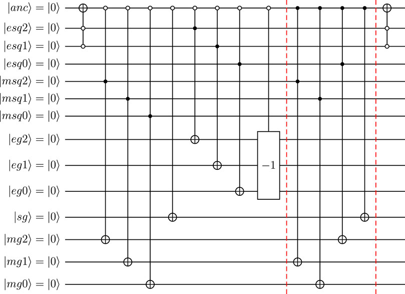
FIGURE 16. Operator 0110 for reduced circuit with 25 or 26 qubits. Squared velocity u₂ defined as quantumfloating-point numbers with N_M = 4 and N_E = 3.

9.3 Reduction including the modulo-adder

Following the analysis of the evaluation of the u² terms in quantum circuits with partial reduction of the workspace qubits, the focus now moves to the more complex case of also reducing the modulo adder (and its reverse) used in computing the summations u + u² and −u + u². The use of 2’s complement method in the current implementation of ${\vec{g}}_{eq}$ evaluation poses particular challenges in the further reduction process, as detailed in this section. In the interest of clarity, this section will consider the reduced circuits for the evaluation of $g_0^{eq}(\left|dv1|dv0\right.⟩=\left|00\right.⟩)$ and $g_3^{eq}(\left|dv1|dv0\right.⟩=\left|00\right.⟩)$, since these represent the only directions for which the modulo-addition steps is required. Figure 17 shows the reduced quantum circuit with 25 qubit resulting from eliminating the three most-significant mantissa qubits in the arithmetic operations for N_M = 4 and N_E = 3. As can be seen, the circuit only involves the mantissa qubit $\left|qu0\right.⟩$. The operation 0011a prepares the modulo-adder step and depends on the mantissa qubits of u as well as on the exponent of u (represented by $\left|eu2|eu1|eu0\right.⟩$). Similarly 0011c un-computes these steps to reset workspace to $\left|0\right.⟩$ after completion of the addition step and setting $g_0^{eq}$ and $g_3^{eq}$ in quantum floating point format. The (reduced) modulo-5 adder MA5 (and its reverse UMA5) only depend on the specific choice of mantissa qubits that were reduced, i.e., in this step there is no dependency on exponent $\left|eu2|eu1|eu0\right.⟩$. Based on the outcome of modulo-5 adder, the operation 0011b sets $g_0^{eq}$ and $g_3^{eq}$ in $\left|mg2|mg1|mg0\right.⟩$ (mantissa), $\left|sg\right.⟩$ (sign) and $\left|eg2|eg1|eg0\right.⟩$ (exponents) for $\left|dv1|dv0\right.⟩=\left|00\right.⟩$ and $\left|dv1|dv0\right.⟩=\left|11\right.⟩$, respectively.

FIGURE 17

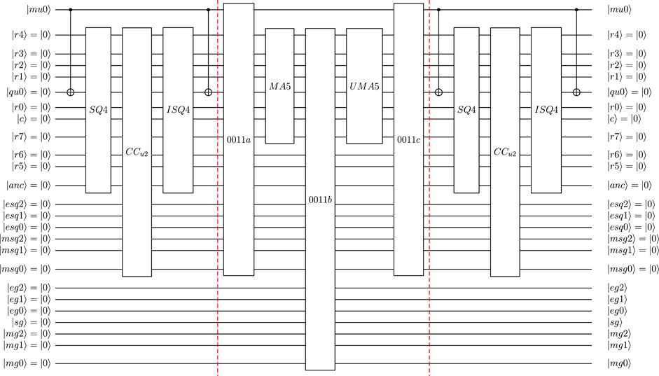
FIGURE 17. Reduced circuit with 25 qubits: $\left|dv1|dv0\right.⟩=\left|00\right.⟩$ or $\left|11\right.⟩$, $\left|eu2|eu1|eu0\right.⟩=\left|011\right.⟩$, $\left|100\right.⟩$, $\left|101\right.⟩$ or $\left|110\right.⟩$ (and therefore $\left|cut\right.⟩=\left|0\right.⟩$).

Following the process detailed in the previous section, for a further reduction by 2 qubits to 26 qubits would result in a similar quantum circuit, then involving $\left|qu1\right.⟩$ and $\left|qu0\right.⟩$. For brevity, this quantum circuit is not shown here.

The operation 0011a comprises two parts. The first part uses quantum-floating point representation of u² to set the “b” register of the modulo-5 Cuccaro adder (i.e., the register that gets overwritten with addition result). Here, a shift is used to account for the difference in exponent of u and u². This part of the 0011a is not affected by the partial reduction of workspace qubits. The second part of 0011a set −u (for $\left|dv1|dv0\right.⟩=\left|00\right.⟩$) or u (for $\left|dv1|dv0\right.⟩=\left|11\right.⟩$) into “a” register of modulo-5 adder. Figure 18 shows the quantum-circuit implementation of this second step before a reduction of workspace qubits is performed. It can be seen that in a partial reduction of the workspace qubits, one or more of the qubits in the “a” register need to be removed. For the example of the reduction to 26 qubits, the qubits $\left|a4|a3|a2\right.⟩$ will be eliminated. For the reduction to 25 qubits, qubits $\left|a4|a3|a2|a1\right.⟩$ will be involved as indicated with the red box in Figure 18.

FIGURE 18

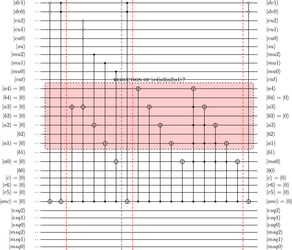
FIGURE 18. Re-arranged quantum circuit (without further reduction on workspace qubits). Quantum circuit shows setting of − u (for $\left|dv1|dv0\right.⟩=\left|00\right.⟩$) or u (for $\left|dv1|dv0\right.⟩=\left|11\right.⟩$) into “a” register of modulo-5 adder. Velocity u and squared velocity u² are defined as quantum floating-point numbers with N_M = 4 and N_E = 3.

The quantum circuit illustrated in Figure 18 first “copies” the mantissa qubits (including the “hidden” qubit) into the “a” register for $\left|dv1|dv0\right.⟩=\left|00\right.⟩$ and for $\left|dv1|dv0\right.⟩$. To perform −u + u², the second part of the circuit transforms the qubits to 2’s complement for $\left|dv1|dv0\right.⟩=\left|00\right.⟩$. Without this change to 2’s complement formulation, i.e., for $\left|dv1|dv0\right.⟩=\left|11\right.⟩$ the reduction of the workspace for the modulo-5 adder can be performed using the approach previously shown for the 4-qubit adders in the evaluation of u².

For $\left|dv1|dv0\right.⟩=\left|00\right.⟩$, in most cases, the need arises to use different computational kernels (derived for different choice of the reduced qubits), depending of the state of the remaining mantissa qubits of u. The following three examples illustrate this:

(1) Reduction by 2 qubits to 26-qubit circuit, $\left|mu2|mu1\right.⟩=\left|0\right.⟩$. For normalized inputs, we then have $\left|qu3|qu2\right.⟩=\left|10\right.⟩$ in the representation without hidden qubit. For $\left|dv1|dv0\right.⟩=\left|00\right.⟩$: “-u” into modulo-5 adder, now 4 cases need to be considered:

• $\left|qu3|qu2|qu1|qu0\right.⟩=\left|1000\right.⟩$ and there for “−u”: $\left|11000\right.⟩$

• $\left|qu3|qu2|qu1|qu0\right.⟩=\left|1001\right.⟩$ and there for “−u”: $\left|10111\right.⟩$

• $\left|qu3|qu2|qu1|qu0\right.⟩=\left|1010\right.⟩$ and there for “−u”: $\left|10110\right.⟩$

• $\left|qu3|qu2|qu1|qu0\right.⟩=\left|1011\right.⟩$ and there for “-u”: $\left|10101\right.⟩$

showing that modulo-5 kernels derived for $\left|a4|a3|a2\right.⟩=\left|110\right.⟩$ and for $\left|a4|a3|a2\right.⟩=\left|101\right.⟩$ are needed, depending on $\left|qu1|qu0\right.⟩$. In addition for $\left|qu0\right.⟩=\left|1\right.⟩$ a NOT operation on $\left|qu1\right.⟩$ just before and after performing the addition is needed;

(2) Reduction by 3 qubits to 25-qubit circuit, $\left|mu2|mu1\right.⟩=\left|00\right.⟩$. For normalized inputs, we then have $\left|qu3|qu2|mu1\right.⟩=\left|100\right.⟩$ in the representation without hidden qubit. For $\left|dv1|dv0\right.⟩=\left|00\right.⟩$: “−u” into modulo-5 adder, now 2 cases need to be considered:

• $\left|qu3|qu2|qu1|qu0\right.⟩=\left|1000\right.⟩$ and there for “−u”: $\left|11000\right.⟩$

• $\left|qu3|qu2|qu1|qu0\right.⟩=\left|1001\right.⟩$ and there for “−u”: $\left|10111\right.⟩$

similar to the reduction-to-26-qubits example, it follows that modulo-5 kernels derived for $\left|a4|a3|a2\right.⟩=\left|1100\right.⟩$ and for $\left|a4|a3|a2\right.⟩=\left|1011\right.⟩$ are needed for this example, again with a switch between these kernels that depends on $\left|qu1|qu0\right.⟩$;

(3) Reduction by 4 qubits to 24-qubit circuit, i.e., with all mantissa qubits for N_M = 4 reduced out in the transformed circuit. For the example $\left|mu2|mu1|mu0\right.⟩=\left|001\right.⟩$, the normalized input showing the hidden qubit is $\left|qu3|qu2|qu1|qu0\right.⟩=\left|1001\right.⟩$. For $\left|dv1|dv0\right.⟩=\left|00\right.⟩$, “−u” is then represented as $\left|10111\right.⟩$

For the first two examples, Figure 19 shows the quantum-circuit implementation of the reduced MA5 operation for $\left|dv1|dv0\right.⟩=\left|00\right.⟩$. The circuits were derived by first creating two separate kernels, e.g. for $\left|a4|a3|a2\right.⟩=\left|110\right.⟩$ and for $\left|a4|a3|a2\right.⟩=\left|101\right.⟩$ in the reduction-by-2 qubits example. Then, the differences between the kernels are performed conditional and ancilla qubit $\left|anc\right.⟩$ in the combined circuits shown.

FIGURE 19

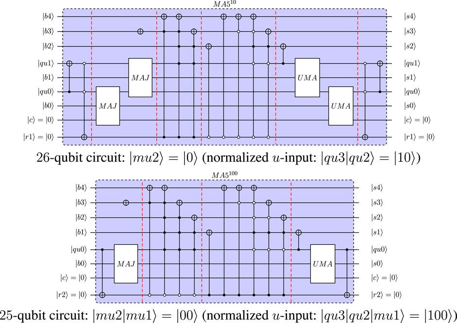
FIGURE 19. Quantum circuits for MA5 used in reduced circuit with 26 qubits and with 25 qubits for $\left|dv1|dv0\right.⟩=\left|00\right.⟩$.

Note: The quantum circuit reductions shown here were performed manually and certainly pose major challenges for automation by circuit compilation methods.

10 Complexity analysis

For the full quantum circuit introduced here, the case with 4 mantissa qubits (N_M = 4) and 3 exponent qubits (N_E = 3) is described in detail in the present work. A crucial factor in applying this quantum algorithm as well as its simulation on classical hardware is its computational complexity in terms of space (number of qubits—or circuit width) and time (number of gate operations and circuit depth) as a function of N_M and N_E. For a well-conditioned computational problem such as the flow field governed by the D1Q3 model (with velocity u, squared velocity u² and re-scaled distribution functions all ≪ 1 in magnitude), it can be expected that meaningful simulations can be performed with N_E = 3. However, to reduce the impact of rounding and truncation errors, realistic applications will involve N_M > 4. Therefore, the growth of circuit width and depth as function of increasing values of N_M is of particular interest in the complexity analysis presented here.

10.1 Full circuit—Before reduction

For the D1Q3 model 2 qubits $\left|dv1|dv0\right.⟩$ are required independent of N_M and N_E. Using the hidden-qubit approach, the u-velocity is defined in terms of exponent, sign and mantissa using N_E + 1 + N_M − 1 = N_E + N_M qubits. For the output ${\vec{g}}^{eq}$, similarly N_E + N_M are required since the same floating-point format is used. A single qubit $\left|cut\right.⟩$ is used to identify cases with truncation to 0 of u². The temporary storage of u² in floating-point representation requires N_E + N_M − 1 qubits since a “sign” qubit is not required. The remaining qubits represent the “workspace” of the algorithm. Two computational steps are performed (as well as their un-computation) within this space: the shift-and-add based evaluation of u² and the “signed” addition ±u + u² for directions $\left|dv1|dv0\right.⟩=\left|00\right.⟩$ and $\left|dv1|dv0\right.⟩=\left|00\right.⟩$. For the example N_M = 4 this addition is performed using a 5-qubit modulo adder. The modulo adder requires 2N_M + 1 qubits. The u² evaluation a 2N_M results register, N_M qubits for unsigned velocity input, 1 “carry” qubit as well as 1 ancilla qubit. In total, the u² evaluation therefore requires 3N_M + 2 qubits. This exceeds the requirement of the modulo adder and therefore the workspace needs a total of 3N_M + 2 qubits. The total space complexity of the original quantum circuit therefore is:

$2+2\left(N_E+N_M\right)+1+\left(N_E+N_M-1\right)+\left(3N_M+2\right)=4+3N_E+6N_M$

10.2 Quantum circuit after reduction steps

After the first reduction step introduced in Section 9, the following qubits were removed from the original circuit: 2 qubits $\left|dv1|dv0\right.⟩$, N_E + N_M (input “u” in signed floating-point format) as well as the single $\left|cut\right.⟩$ qubit. Therefore, the total space complexity for the quantum circuit following this first reduction step is therefore:

$4+3N_E+6N_M-\left[2+\left(N_E+N_M\right)+1\right]=1+2N_E+5N_M$

The further reduction detailed in Section 9.1, one or more of the N_M qubits defining the unsigned velocity input into the u² evaluation were eliminated. In its most aggressive form, this reduction step can eliminate all N_M qubits defining the unsigned velocity input, so that the space complexity reduces further to:

$1+2N_E+5N_M-N_M=1+2N_E+4N_M$

To illustrate the complexity for different choices of N_M, Table 3 summarized the required number of qubits for N_E = 3 and increasing N_M for the original quantum circuits as well as the reduction steps 1 and 2.

TABLE 3

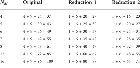
TABLE 3. Required number of qubits for original and transformed quantum circuits (N_E = 3).

Figure 20 shows the memory required to store the qubit information as a pair of 32-bit floating point numbers. For reference, the red lines show the FPGA board memory and 1 TB, 1 PB, 1 EB and 1 ZB. To put this into context: the UK’s largest supercomputer, Archer, comprises 4,920 nodes with each 64 GB of memory, so the total memory is still less than 1 PB.

FIGURE 20

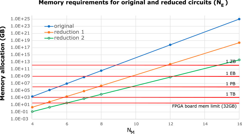
FIGURE 20. Memory requirements for the original circuit and the two types of reduced circuits as a function of N_M, for N_E = 3

11 Examples of D1Q3 quantum circuit reduced to 25 qubits

In this section, two examples are considered of reduced circuits with 25 qubits:

• Example 1: velocity u defined as $\left|01000|110\right.⟩=+8/32=+1/4$ or $\left|01001|110\right.⟩=+9/32$. Alternatively, in terms of unsigned hidden-qubit formulation for mantissa: $\left|mu2|mu1|mu0|eu2|eu1|eu0\right.⟩=\left|000|110\right.⟩$ or $\left|mu2|mu1|mu0|eu2|eu1|eu0\right.⟩=\left|001|110\right.⟩$;

• Example 2: velocity u defined as $\left|01100|101\right.⟩=+12/64=+3/16$ or $\left|01101|101\right.⟩=+13/64$. In terms of unsigned hidden-qubit formulation for mantissa: $\left|mu2|mu1|mu0|eu2|eu1|eu0\right.⟩=\left|100|101\right.⟩$ or $\left|mu2|mu1|mu0|eu2|eu1|eu0\right.⟩=\left|101|101\right.⟩$.

With a further reduction by 3 qubits, this means that only $\left|mu0\right.⟩$ acts as input qubit, and therefore the reduced circuits represented by both examples only compute 2 separate input velocities u each, as itemized above.

The equilibrium distribution functions $g_0^{eq}$ (defined by $\left|dv1|dv0\right.⟩=\left|00\right.⟩$) and $g_3^{eq}$ (defined by $\left|dv1|dv0\right.⟩=\left|11\right.⟩$) are shown in Table 4.

TABLE 4

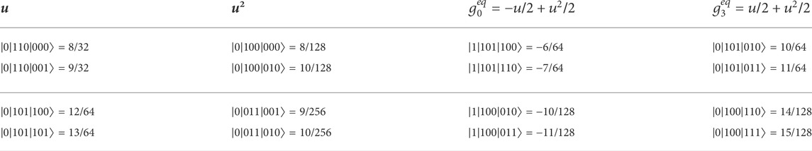
TABLE 4. Input and output of examples for 25-qubit example circuits. Mantissa is shown without “hidden qubit.”

Here, the term −u + u² required in $g_0^{eq}$ was evaluated as follows using a modulo-5 adder. For positive numbers, a 5-qubit input with a leading $\left|0\right.⟩$, followed by the hidden qubit and N_M − 1 = 3 mantissa qubits is used, while for negative numbers, the 4-qubit representation (including hidden qubit) is transformed into its 5-qubit 2’s complement. Furthermore, mantissa qubits are shifted where necessary to account for difference in exponents of the two inputs. Such shifts are performed before transformation to 2’s complement. Then, for the four examples in the table above, the “signed” addition can be summarized as:

$\begin{array}{ccc}\hfill u=8/32& \left(\left|0|110|000\right.⟩\right):\hfill & \left|11000\right.⟩+\left|00010\right.⟩=\left|11010\right.⟩\to -u+u^2=\left|1|101|100\right.⟩=-6/32=-12/64\hfill \\ \hfill u=9/32& \left(\left|0|110|001\right.⟩\right):\hfill & \left|10111\right.⟩+\left|00010\right.⟩=\left|11001\right.⟩\to -u+u^2=\left|1|101|110\right.⟩=-7/32=-14/64\hfill \\ \hfill u=12/64& \left(\left|0|101|100\right.⟩\right):\hfill & \left|10100\right.⟩+\left|00010\right.⟩=\left|10110\right.⟩\to -u+u^2=\left|1|101|010\right.⟩=-10/64\hfill \\ \hfill u=13/64& \left(\left|0|101|101\right.⟩\right):\hfill & \left|10011\right.⟩+\left|00010\right.⟩=\left|10101\right.⟩\to -u+u^2=\left|1|101|011\right.⟩=-11/64\hfill \end{array}$

As can be seen, in the top two examples, the outcomes −6/32 and −7/32 result from the modulo-5 mantissa addition, so that a re-normalization is required. This leads to the normalized numbers −12/64 and −14/64, respectively. For the bottom two examples, such a re-normalization was not required.

12 Evaluation

12.1 Experimental setup

We evaluated our approach on a single-node FPGA system. Our host system has a dual Intel Xeon E5-2609 V2 2.5 GHz processor and 64 GB RAM (DDR3, 1.6 GHz). This system hosts a Nallatech PCIe-385N A7 FPGA board with 8 GB RAM (DDR3) connected through a PCIe 2 connection. The system runs Scientific Linux 6.8 and we used the Intel SDK for OpenCL Version 17.1 to communicate with and program the FPGA device. The CPU used for evaluation is the same as the FPGA host. The host code is compiled using G++ (GCC version 4.7.2). To evaluate the CPU approach, we run the same OpenCL kernel with the same host code. Our GPU system has access to an NVIDIA GK110B (GeForce GTX TITAN Black), with access to 6 GB of VRAM, which is used for the GPU evaluation target. The GPU system compiles the C++ host code with G++ (GCC version 5.4.0).

12.2 Experimental results

12.2.1 FPGA resource utilization

We compiled our source code with the AOC tool provided by the Intel SDK for OpenCL. Table 5 summarizes the FPGA resource utilization and maximum operating frequency (F_max) after synthesis for the presented architecture for 1 through 8 compute units. We see that while we cannot double our current maximum number of compute units directly, we still have room to improve the design by simply adding more compute units, potentially up to 12 units. This is still to be demonstrated as adjustments have to be made to allow for a non-power of 2 number of compute units.

TABLE 5

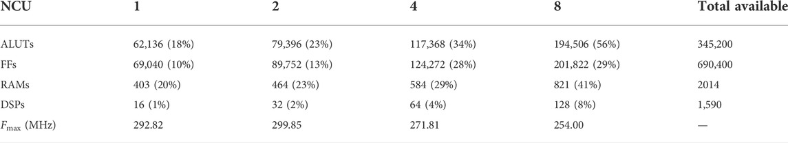
TABLE 5. FPGA resource utilization and maximum frequency for a baseline (Over-PCIe) Single-Qubit gate QWM kernel for 1 through 8 compute units and 8 maximum controls per gate.

12.2.2 Full square circuits

Figure 21 shows the runtime results for several full squaring circuits with input mantissa sizes of 4 bits through 8 bits. The FPGA outperforms the CPU for a small number of qubits, which is demonstrative of the higher overhead needed by the CPU to run the circuit. For a higher number of qubits, the CPU clearly outperforms our current baseline FPGA implementation. This is down to the current implementation not having any FPGA-specific optimizations (discussed below). In particular, to achieve universality, this architecture can run a number of different gates based on the gate opcode (or gate matrix) passed to it by the host. While this is necessary for some algorithms which require universality, some classes of circuits can be performed with a reduced set of operational gates, for which we can specialize the FPGA architecture. Aminian et al. (2008) demonstrate this in their work discussed in Section 3.2.

FIGURE 21

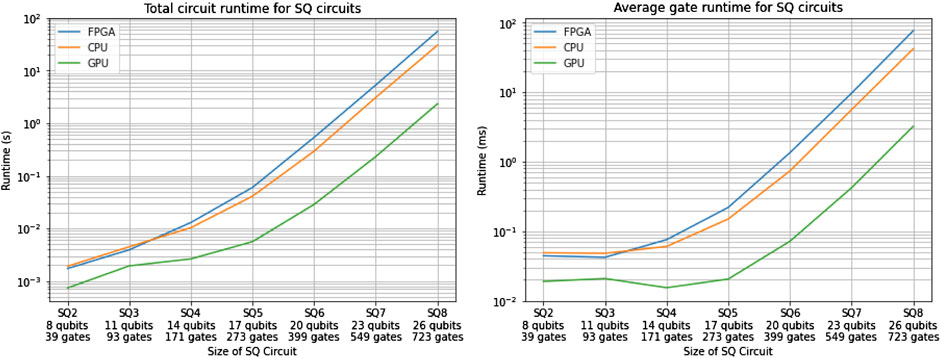
FIGURE 21. Total circuit and average gate simulation times for the squaring circuits with different input sizes. Logarithmic scale is representative of growing circuit qubit count.

12.2.3 Reduced square circuits

Figure 22 shows the runtime results for the full 4-bit input mantissa squaring circuit and two reduced specializations with three fewer qubits. As expected, the lower qubit reduced circuits outperform the full circuit and require considerably less memory. This demonstrates the advantage in runtime gained by performing the proposed reductions on a small circuit. For the two demonstrated reduced circuits, the FPGA slightly outperforms the CPU, which again is down to the CPU having more overhead. This will not be the case for a larger circuit being simulated on this baseline architecture.

FIGURE 22

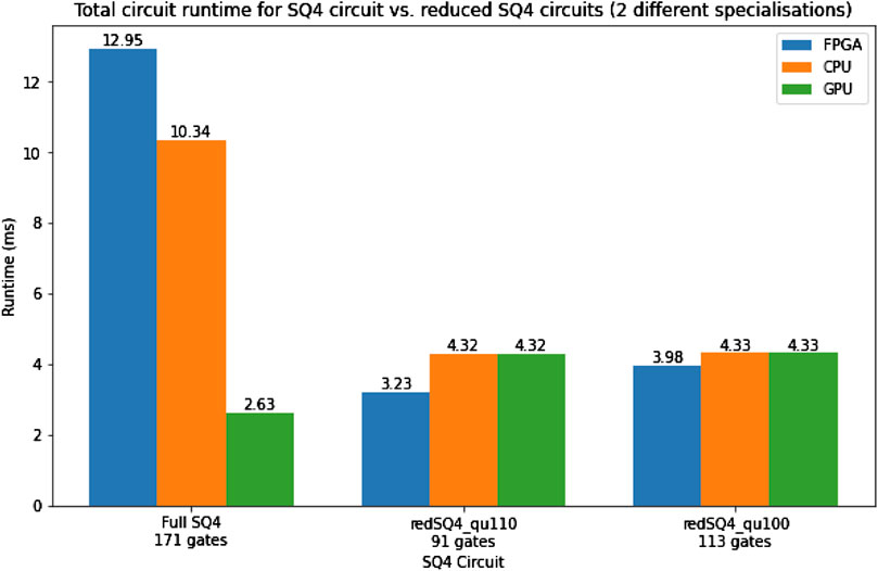
FIGURE 22. Total circuit simulation times for the full SQ4 and the reduced SQ4 circuit with two different input specializations.

12.2.4 Reduced 25-qubit D1Q3

Figure 23 shows the total circuit runtime results for the reduced 25-qubit D1Q3 with several specializations for $\left|d{v}_1|d{v}_0\right.⟩$ and $\left|e{u}_2|e{u}_1|e{u}_0\right.⟩$. The observed variations in total circuit runtime between the different specializations of the D1Q3 circuit are due to the number of quantum gates being different across these specialized reduced circuits. Because of the memory restrictions of our CPU and FPGA systems, we were unable to run the full 37-qubit version of this circuit. In this work, the main motivation for the introduced circuit transformations is to facilitate the simulation of large circuits, which without these reductions would not fit in the memory. Alternatively, similar transformations can also be used on smaller circuits that do fit in the device’s memory to reduce their execution times, by taking advantage of fine-grained parallelism, as demonstrated in the previous section. For evaluating the circuit for different inputs, different quantum circuit specializations have to be ran on the architecture; however, since the architecture is circuit-independent, there is no extra cost for running different circuits on it. Since no FPGA bitstream compilation has to be run between circuit evaluations, this achieves our goal of reusability, up to some constant maximum number of controls per gate.

FIGURE 23

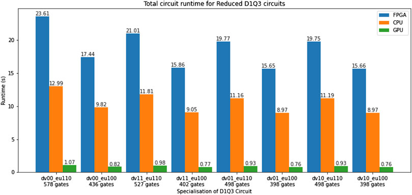
FIGURE 23. Total circuit simulation times for the reduced D1Q3 circuit with different input specializations.

12.3 Discussion

The above results show the potential of our approach of circuit transformations to reduce the number of qubits in exchange for a higher number of control bits. Table 6 shows a summary of the runtimes used to infer the following performance and power consumption results. With the current status of our work, in absolute terms, the performance of the simulation on the FPGA is about half as fast as on the CPU host. The GPU benefits from very high memory bandwidth and thousands of compute threads, and thus it shines for this particular approach of simulation (QWM with a full state vector), beating the FPGA by a factor of 20 for high-qubit circuits.

TABLE 6

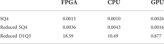
TABLE 6. Runtime results in seconds for architecture with 8 NCU and 8 NCONTROLS. Displayed results for reduced circuits is the average runtime across different specializations, which vary in circuit width.

However, as explained before, to scale to larger numbers of qubits, it is necessary to move to clusters of FPGAs. For supercomputer clusters, the dominant factor is the energy consumption and therefore we need to consider the performance per Watt. From that perspective, the picture is quite different: the measured power consumption of the FPGA board is 25 W (Segal et al., 2014); the host CPU consumes 160 W (not including RAM power consumption). So already the FPGA simulation has more than 3× better performance per Watt than the CPU. Our evaluation GPU consumes 250 W of power, meaning it is about 2× better than the FPGA in terms of performance per Watt.

12.4 Future further improvements

Furthermore, there is a lot of scope for improvement of the FPGA performance. We used a baseline over-PCIe architecture without pipeline control to obtain the presented results. For parallelisation on the device, the architecture currently relies on the dynamic scheduler of the OpenCL NDRange construct. It is unclear how well this pipelines our design and we estimate the architecture would likely benefit from tighter control over pipelining. This would involve using OpenCL channels to explicitly control the flow of the amplitudes through the design. In addition, we are currently not applying any caching techniques in our design, several of which can be applied. Each of our kernels currently reads two values at a time from the distributed RAM of the FPGA, performs some computation on them, and writes them back. We can make better utilization of the DRAM’s bandwidth by reading the required amplitudes in consecutive blocks. Due to the exponential strides between the amplitudes, it may not always be possible to fill the cache in one memory read with matching amplitudes. However, we can show that this is possible with two contiguous memory reads. Furthermore, another optimization technique which would be particularly useful for circuits like the ones presented here is state vector compression. For circuits whose intermediary state vectors present repetition in their amplitude values, it is not always necessary to store the full state vector in memory. Instead, memory access is replaced by computation over a compressed state vector space; a pattern very suitable for application on an FPGA.

With these improvements, which are the focus of our research at the moment, it is expected that the FPGA will outperform the CPU even in absolute terms, so that we are confident that the FPGA simulation can achieve an order of magnitude better performance per Watt. We are also aiming to show that an optimized FPGA architecture can outperform a GPU in performance per Watt and total energy consumption.

13 Conclusion

Quantum circuits for the non-linear equilibrium distribution function for the D1Q3 lattice-based model were introduced as a step towards more complete models such as D2Q9 and D3Q27. A key feature of the derived circuits is the use of the quantum computational basis encoding along with the use of a reduced-precision floating-point representation. This in contrast to existing work typically employing fixed-point representation in quantum algorithms using the quantum computational basis encoding. It is demonstrated that for modest precision (e.g., using 4-bit mantissas) quantum circuits with fewer than 40 qubits can be derived. Even with further ancillae qubits that result from transpiling the circuit to native gates available on quantum hardware, this shows that for Noisy Intermediate-Scale Quantum (NISQ) Computer-era hardware, demonstration of the introduced quantum circuits is feasible. The quantum-circuit transformation introduced and detailed in this work show that starting from the full circuit, reduced circuits can effectively be created so that step-by-step the behavior of the full quantum circuit can be analyzed using more limited resources, while taking advantage of the fine-grained parallelism offered by FPGAs.

We demonstrate reductions from 37 to 23 qubits for the quantum circuit computing the equilibrium distribution function of D1Q3 model with input velocity defined in floating-point format with a 4-qubit mantissa and 3-qubit exponent. For increased mantissa qubit count of 16, a reduction from 109 to 71 qubits occurs. We show that the reduced circuit can be successfully run on an FPGA system and that the FPGA simulation has more than 3× better performance per Watt compared to the CPU simulation.

In future work, the quantum-circuit transformation methods will be analyzed further and extended to wider range of circuits. In terms of fluid dynamics applications, the step towards D2Q9 and D3Q27 is the aim of future work. We will also explore a number of techniques to improve the FPGA simulation performance, with the aim of obtaining a 10× improvement in performance per Watt over the CPU and outperforming the GPU in energy consumption.

Data availability statement

The raw data supporting the conclusion of this article will be made available by the authors, without undue reservation.

Author contributions

YM: Development of Haskell compilation toolchain and FPGA architecture—Presenting results of encoded reduced quantum circuits for D1Q3 and analysis WV: Summary and discussion of presented results and power efficiency analysis RS: Derivation of the quantum circuit implementation of the D1Q3 model—Initiated the work on the circuit transformation methods for reducing required number of qubits—Manual derivation of the example reduced circuits provided.

Funding

This work was supported by a PhD studentship from the College of Science and Engineering at the University of Glasgow.

Conflict of interest

The authors declare that the research was conducted in the absence of any commercial or financial relationships that could be construed as a potential conflict of interest.

Publisher’s note

All claims expressed in this article are solely those of the authors and do not necessarily represent those of their affiliated organizations, or those of the publisher, the editors and the reviewers. Any product that may be evaluated in this article, or claim that may be made by its manufacturer, is not guaranteed or endorsed by the publisher.

References

Aaronson, S., and Gottesman, D. (2004). Improved simulation of stabilizer circuits. Phys. Rev. A 70, 052328. doi:10.1103/PhysRevA.70.052328

CrossRef Full Text | Google Scholar

Aïmeur, E., Brassard, G., and Gambs, S. (2007). “Quantum clustering algorithms,” in ICML ’07: Proceedings of the 24th International Conference on Machine Learning (New York, NY, USA: Association for Computing Machinery), 1–8. doi:10.1145/1273496.1273497

CrossRef Full Text | Google Scholar

Aminian, M., Saeedi, M., Zamani, M. S., and Sedighi, M. (2008). “FPGA-based circuit model emulation of quantum algorithms,” in 2008 IEEE Computer Society Annual Symposium on VLSI (Montpellier, France: IEEE), 399–404. doi:10.1109/ISVLSI.2008.43

CrossRef Full Text | Google Scholar

Aramon, M., Rosenberg, G., Valiante, E., Miyazawa, T., Tamura, H., and Katzgraber, H. G. (2019). Physics-inspired optimization for quadratic unconstrained problems using a digital annealer. Front. Phys. 7. doi:10.3389/fphy.2019.00048

CrossRef Full Text | Google Scholar

Berman, G., Ezhov, A., Kamenev, D., and Yepez, J. (2002). Simulation of the diffusion equation on a type-II quantum computer. Phys. Rev. A 66, 012310. doi:10.1103/PhysRevA.66.012310

CrossRef Full Text | Google Scholar

Berry, D., Childs, A., Ostrander, A., and Wang, G. (2017). Quantum algorithm for linear differential equations with exponentially improved dependence on precision. Commun. Math. Phys. 356, 1057–1081. doi:10.1007/s00220-017-3002-y

CrossRef Full Text | Google Scholar

Berry, D. (2014). High-order quantum algorithm for solving linear differential equations. J. Phys. A Math. Theor. 47, 105301. doi:10.1088/1751-8113/47/10/105301

CrossRef Full Text | Google Scholar

Bonny, T., and Haq, A. (2020). Emulation of high-performance correlation-based quantum clustering algorithm for two-dimensional data on FPGA. Quantum Inf. process. 19, 179. doi:10.1007/s11128-020-02683-9

CrossRef Full Text | Google Scholar

Budinski, L. (2021). Quantum algorithm for the advection–diffusion equation simulated with the lattice Boltzmann method. Quantum Inf. process. 20, 57. doi:10.1007/s11128-021-02996-3

CrossRef Full Text | Google Scholar

Cao, Y., Papageorgiou, A., Petras, I., Traub, J., and Kais, S. (2013). Quantum algorithm and circuit design solving the Poisson equation. New J. Phys. 15, 013021. doi:10.1088/1367-2630/15/1/013021

CrossRef Full Text | Google Scholar

Childs, A., and Liu, J. (2020). Quantum spectral methods for differential equations. Commun. Math. Phys. 375, 1427–1457. doi:10.1007/s00220-020-03699-z

CrossRef Full Text | Google Scholar

Conceicao, C., and Reis, R. (2015). “Efficient emulation of quantum circuits on classical hardware,” in 2015 IEEE 6th Latin American Symposium on Circuits & Systems (LASCAS) (Montevideo, Uruguay: IEEE), 1–4. doi:10.1109/LASCAS.2015.7250404

CrossRef Full Text | Google Scholar

Costa, P., Jordan, S., and Ostrander, A. (2019). Quantum algorithm for simulating the wave equation. Phys. Rev. A . Coll. Park. 99, 012323. doi:10.1103/PhysRevA.99.012323

CrossRef Full Text | Google Scholar

Steijl, R. (2020). “Quantum algorithms for fluid simulations,” in Advances in quantum communication and information. Editor F. Bulnes (London: IntechOpen). ISBN 9781789852684. doi:10.5772/intechopen.86685

CrossRef Full Text | Google Scholar

Steijl, R. (2022). “Quantum algorithms for nonlinear equations in fluid mechanics,” in Quantum computing and communications. Editor Y. Zhao (London: IntechOpen). ISBN 9781839681332. doi:10.5772/intechopen.95023

CrossRef Full Text | Google Scholar

De Raedt, H., Hams, A. H., Michielsen, K., and De Raedt, K. (2000). Quantum computer emulator. Comput. Phys. Commun. 132, 1–20. doi:10.1016/S0010-4655(00)00132-6

CrossRef Full Text | Google Scholar

De Raedt, K., Michielsen, K., De Raedt, H., Trieu, B., Arnold, G., Richter, M., et al. (2007). Massively parallel quantum computer simulator. Comput. Phys. Commun. 176, 121–136. doi:10.1016/j.cpc.2006.08.007

CrossRef Full Text | Google Scholar

Fillion-Gourdeau, F., and Lorin, E. (2019). Simple digital quantum algorithm for symmetric first-order linear hyperbolic systems. Numer. Algorithms 82, 1009–1045. doi:10.1007/s11075-018-0639-3

CrossRef Full Text | Google Scholar

Gaitan, F. (2020). Finding flows of a Navier–Stokes fluid through quantum computing. npj Quantum Inf. 6, 61. doi:10.1038/s41534-020-00291-0

CrossRef Full Text | Google Scholar

Garcia, H., and Markov, I. (2015). Simulation of quantum circuits via stabilizer frames. IEEE Trans. Comput. 64, 2323–2336. doi:10.1109/TC.2014.2360532

CrossRef Full Text | Google Scholar

[Dataset] García-Molina, P., Rodríguez-Mediavilla, J., and García-Ripoll, J. J. (2021). Solving partial differential equations in quantum computers.

Google Scholar

García-Ripoll, J. J. (2021). Quantum-inspired algorithms for multivariate analysis: From interpolation to partial differential equations. Quantum 5, 431. doi:10.22331/q-2021-04-15-431

CrossRef Full Text | Google Scholar

Green, A. S., LeFanu, P., Ross, N. J., Selinger, P., and Valiron, B. (2013). Quipper: A scalable quantum programming language. arXiv.org, 1304:3390.

Google Scholar

Gutiérrez, E., Romero, S., Trenas, M. A., and Zapata, E. L. (2010). Quantum computer simulation using the cuda programming model. Comput. Phys. Commun. 181, 283–300. doi:10.1016/j.cpc.2009.09.021

CrossRef Full Text | Google Scholar

Han, K., and Kim, J. (2002). Quantum-inspired evolutionary algorithm for a class of combinatorial optimization. IEEE Trans. Evol. Comput. 6, 580–593. doi:10.1109/TEVC.2002.804320

CrossRef Full Text | Google Scholar

Harrow, A., Hassidim, A., and Lloyd, S. (2009). Quantum algorithm for linear systems of equations. Phys. Rev. Lett. 103, 150502. doi:10.1103/PhysRevLett.103.150502

PubMed Abstract | CrossRef Full Text | Google Scholar

Itani, W., and Succi, S. (2022). Analysis of carleman linearization of lattice Boltzmann. Fluids 7, 24. doi:10.3390/fluids7010024

CrossRef Full Text | Google Scholar

Kelly, A. (2018). Simulating quantum computers using OpenCL. arXiv:1805.00988 [quant-ph]. ArXiv: 1805.00988.

Google Scholar

Kerenidis, I., and Prakash, A. (2020). Quantum gradient descent for linear systems and least squares. Phys. Rev. A 101, 022316. doi:10.1103/PhysRevA.101.022316

CrossRef Full Text | Google Scholar

Khalid, A., Zilic, Z., and Radecka, K. (2004). “FPGA emulation of quantum circuits,” in IEEE International Conference on Computer Design: VLSI in Computers and Processors, 2004. ICCD 2004. Proceedings (San Jose, CA, USA: IEEE), 310–315. doi:10.1109/ICCD.2004.1347938

CrossRef Full Text | Google Scholar

Khalid, M., Mujahid, U., Jafri, A., Choi, H., and Muhammad, N. (2021). An FPGA-based hardware abstraction of quantum computing systems. J. Comput. Electron. 20, 2001–2018. doi:10.1007/s10825-021-01765-w

CrossRef Full Text | Google Scholar

[Dataset] Knudsen, M., and Mendl, C. B. (2020). Solving differential equations via continuous-variable quantum computers.

Google Scholar

Lee, Y., Khalil-Hani, M., and Marsono, M. (2016). An FPGA-based quantum computing emulation framework based on serial-parallel architecture. Int. J. Reconfigurable Comput. 18, 1. doi:10.1155/2016/5718124

CrossRef Full Text | Google Scholar

Lee, Y., Khalil-Hani, M., and Marsono, M. (2018). Improved quantum circuit modelling based on Heisenberg representation. Quantum Inf. process. 17 (36), 36–28. doi:10.1007/s11128-017-1806-5

CrossRef Full Text | Google Scholar

[Dataset] Leyton, S., and Osborne, T. (2008). A quantum algorithm to solve nonlinear differential equations.

Google Scholar

[Dataset] Liu, J. P., Øie Kolden, H., Krovi, H. K., Loureiro, N. F., Trivisa, K., and Childs, A. M. (2021). Efficient quantum algorithm for dissipative nonlinear differential equations.

Google Scholar

[Dataset] Lloyd, S., Palma, G. D., Gokler, C., Kiani, B., Liu, Z. W., Marvian, M., et al. (2020). Quantum algorithm for nonlinear differential equations.

Google Scholar

Lu, X., Yuan, J., and Zhang, W. (2013). Workflow of the grover algorithm simulation incorporating cuda and gpgpu. Comput. Phys. Commun. 184, 2035–2041. doi:10.1016/j.cpc.2013.03.017

CrossRef Full Text | Google Scholar

Ma, G., Li, H., and Zhao, J. (2020). Quantum qr decomposition in the computational basis. Quantum Inf. process. 19, 271. doi:10.1007/s11128-020-02777-4

CrossRef Full Text | Google Scholar

Mahmud, N., and El-Araby, E. (2019). Dimension reduction using Quantum Wavelet Transform on a high-performance reconfigurable computer. Int. J. Reconfigurable Comput. 2019, 1. doi:10.1155/2019/1949121

CrossRef Full Text | Google Scholar

Mahmud, N., Haase-Divine, B., Kuhnke, A., Rai, A., MacGillivray, A., and El-Araby, E. (2020). Efficient computation techniques and hardware architectures for unitary transformations in support of quantum algorithm emulation. J. Signal Process. Syst. 92, 1017–1037. doi:10.1007/s11265-020-01569-4

CrossRef Full Text | Google Scholar

Montanaro, A., and Pallister, S. (2016). Quantum algorithms and the finite element method. Phys. Rev. A 93, 032324. doi:10.1103/PhysRevA.93.032324

CrossRef Full Text | Google Scholar

Nielsen, M., and Chuang, I. (2010). Quantum computation and quantum information. 10th Anniversary Edition. Cambridge: Cambridge University Press.

Google Scholar

Pilch, J., and Dlugopolski, J. (2019). An FPGA-based real quantum computer emulator. J. Comput. Electron. 18, 329–342. doi:10.1007/s10825-018-1287-5

CrossRef Full Text | Google Scholar

Rosenbaum, D. (2010). Binary superposed quantum decision diagrams. Quantum Inf. process. 9, 463–496. doi:10.1007/s11128-009-0153-6

CrossRef Full Text | Google Scholar

Scherer, A., Valiron, B., Mau, S., Alexander, S., van den Berg, E., and Chapuran, T. (2017). Concrete resource analysis of the quantum linear-system algorithm used to compute the electromagnetic scattering cross section of a 2D target. Quantum Inf. process. 16, 60. doi:10.1007/s11128-016-1495-5

CrossRef Full Text | Google Scholar

Segal, O., Nasiri, N., Margala, M., and Vanderbauwhede, W. (2014). “High level programming of fpgas for hpc and data centric applications,” in 2014 IEEE High Performance Extreme Computing Conference (HPEC) (IEEE), 1–3.

CrossRef Full Text | Google Scholar

Steijl, R., and Barakos, G. (2018). Parallel evaluation of quantum algorithms for computational fluid dynamics. Comput. Fluids 173, 22–28. doi:10.1016/j.compfluid.2018.03.080

CrossRef Full Text | Google Scholar

Tabakin, F., and Julia-Diaz, B. (2009). Qcmpi: A parallel environment for quantum computing. Comput. Phys. Commun. 180, 948–964. doi:10.1016/j.cpc.2008.11.021

CrossRef Full Text | Google Scholar

Todorova, B., and Steijl, R. (2020). Quantum algorithm for the collisionless Boltzmann equation. J. Comput. Phys. 409, 109347. doi:10.1016/j.jcp.2020.109347

CrossRef Full Text | Google Scholar

Viamontes, G., Markov, I., and Hayes, J. (2003). Improving gate-level simulation of quantum circuits. Quantum Inf. process. 2, 347–380. doi:10.1023/b:qinp.0000022725.70000.4a

CrossRef Full Text | Google Scholar

Xu, G., Daley, A., Givi, P., and Somma, R. (2018). Turbulent mixing simulation via a quantum algorithm. AIAA J. 56, 687–699. doi:10.2514/1.J055896

CrossRef Full Text | Google Scholar

Xue, C., Wu, Y.-C., and Guo, G.-P. (2021). Quantum homotopy perturbation method for nonlinear dissipative ordinary differential equations. New J. Phys. 23, 123035. doi:10.1088/1367-2630/ac3eff

CrossRef Full Text | Google Scholar

Yepez, J. (2001). Quantum lattice-gas model for computational fluid dynamics. Phys. Rev. E 63, 046702. doi:10.1103/PhysRevE.63.046702

PubMed Abstract | CrossRef Full Text | Google Scholar

Zhou, S., Loke, T., Izaac, J., and Wang, J. (2017). Quantum fourier transform in computational basis. Quantum Inf. process. 16, 82. doi:10.1007/s11128-017-1515-0

CrossRef Full Text | Google Scholar