Dynamic analysis and validation of a multi-body floating wind turbine using the moving frame method

1 Introduction

The world’s increasing need for energy makes renewable energy sources attractive. While the demand for renewable energy increases, so does the resistance to onshore wind farms due to the environmental impact, which puts certain species at risk WWF (2022). Offshore wind farms will lessen the environmental impact regarding permanent structures’ installation and yield more favourable wind conditions Burton et al. (2011).

Floating offshore wind turbines (FOWT), however, experience harsher environmental loads and also increased freedom to translate compared to fixed installations. This implies that predicting the movement of the FOWT is a challenge unto itself. To maximise their potential, continually improved analyses for floating offshore wind farms must be implemented.

Currently, there exists reliable commercial software to conduct analyses of such structures. However, as engineers continue to infuse analyses with artificial intelligence, it is advisable to rely on such legacy software alone and, instead, supplement analyses with A.I. and digital twins. A digital twin is a representation of an industrial asset in operation that includes the asset’s condition and relevant historical data. When supplemented with AI, such models can vastly improve the asset’s operation; in this case, includes the modelling of dynamics response. A judicious use of inter-process communication algorithms, in which a digital twin can access a database of both previously solved problems coupled with extant weather conditions; and this can speed the computation for near real-time simulations. In fact, this work is currently underway in a related project of crane motion on ships using the method used and discussed herein.

The Moving Frame Method (MFM) can ease the process of obtaining the equations of motion Storaas et al. (2019) and can substantially reduce simulation time when implemented without the computational overhead of commercial software. The MFM utilizes Lie algebra and Cartan’s notion of Moving frames to extract the equations of motion of both single- and multi-body systems as well as 2D and 3D kinetics in a consistent notational matter Impelluso (2017).

This research constructs the equations of motion using the MFM and implements some of the environmental loads. It will focus on the OC3 Phase IV spar-buoy platform and the NREL 5MW reference turbine due to extensive research already performed on such platforms and turbines. The goal is to replicate previously found results and also to lay the foundation for further use of the MFM when addressing complex multi-body dynamic systems. The authors selected the FOWT as such an implementation due to its nature. It is a complex machine, and experiences equally complex loading. Furthermore, the industry is implementing AI for many of its optimization problems. This makes the MFM method an interesting approach to use. Essentially, this project endeavors to demonstrate advanced computational techniques, such as how the MFM enables easy transitions between scenarios where the tower-nacelle-rotor connection is considered as a rigid body, and, later, coupled with a finite element process, a deformable body.

To understand the method, the reader may review two papers Impelluso (2017); Murakami (2013). In the first half of this paper, we will launch directly into the method in a tutorial style.

2 The moving frame method

The Moving Frame Method (MFM) represents a paradigm shift in the foundation of the discipline of multi-body dynamics.

2.1 MFM background

The MFM exploits the philosophy of Elie Cartan who advocated that all objects be endowed with a moving reference frame Cartan (1986). To relate the moving frames in a multi-body system (one for each link), the MFM utilizes a compact notation, along with the group theory and associated algebra of Sophus Lie but distilled to the simplicity of matrix multiplications Frankel (2011).

In addition, the MFM for multi-bodies adopts a revised approach to the Principle of Virtual work, in which a proper variation of the angular velocity is established. While Wittenburg Wittenburg (2007) advocated the use of virtual power to embed driving forces and motor torques into the variation principle, the MFM adopts a restriction on the variation of the angular velocity. This restriction derives from both the variation of the frame and the variation of the coordinates; and as first advocated by Holm Holm (2008).

The MFM is not merely an alternate method of analysis. Rather, it represents a paradigm shift in a discipline—one which empowers the moving reference frame over the inertial. It eschews the notion of fictious forces that derive from such frames, and predicating itself on the reality that everything moves. The MFM renders a notation that is consistent across the facets of dynamics. It enables 2D, 3D, single and multi-body dynamics to be represented with the same consistent notation. It needs no validation as it produces the same equations of motion as the traditional approach to dynamics, but more expeditiously, and with a suite of equations that more more amenable to coding through its matrix-based formulation.

A pedagogical analysis of the method and an assessment of student learning has been presented previously Impelluso (2017) for single body, 3D dynamics. Regarding research, the MFM has been used to model ROV motion Austefjord et al. (2018), friction Rykkje et al. (2021), gyroscopic wave energy converters Korsvik et al. (2019), a knuckle boom crane Eia et al. (2019), and ship stability Flatlandsmo et al. (2019).

In this project, we apply the MFM to study the dynamics of a wind turbines. In this way, we demonstrate the power of the MFM and its ability for easy deployment in the analysis of floating wind turbines. For in this era of smart machines, we must consider recoding legacy software if we are to imbue existing software with artificial intelligence.

2.2 Applying the moving frame method

Figure 1 illustrates how each body of the FOWT will be endowed with its own reference frame at the body’s center of mass. The combined body of the platform and the tower will hold the first frame from which the inertial frame will be deposited. In other words, the first body’s frame is primary and the inertial frame is merely a decal to be peeled off at the onset of the analysis to compute position data. The second moving reference frame is attached to the nacelle, and the third is attached to the combined body of the hub and the blades. All frames will be aligned with the centre of mass of the respective bodies at the start time. In the following section, the kinematics of each moving frame will be described. This will lay the foundation for obtaining the equations of motion. We now use the Special Euclidean Group, SE(3), to obtain each component’s angular velocity and translational velocities systematically. However, to ease understanding, the reader is advised to consult the primary results of each of the following three subsections, as per Table 1, below:

FIGURE 1

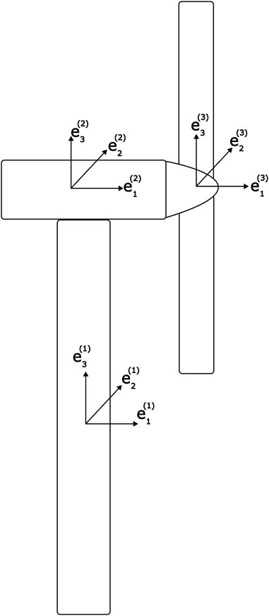
FIGURE 1. Turbine with frames attached to each body.

TABLE 1

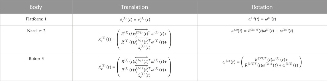
TABLE 1. Kinematic results.

2.3 Kinematics of the platform, body 1

The platform will have all rotational and translational freedoms.

• The rotation of the platform—pitch, yaw and roll—from the inertial frame, is found by post-multiplying the inertial frame by a rotation (a member of the special orthogonal group, SO(3).

• The translation of the platform—surge, heave and sway from the inertial frame is found by post-multiplying the inertial frame by translation coordinates.

${\mathbf{e}}^{\left(1\right)}\left(t\right)={\mathbf{e}}^I{R}^{\left(1\right)}\left(t\right)(1)$

${\mathbf{r}}_c^{\left(1\right)}\left(t\right)={\mathbf{e}}^I{x}_c^{\left(1\right)}\left(t\right)(2)$

Obtaining these rotational and translational coordinates in the inertial reference frame will be the main focus of later parts of the analysis. However, at this time, we proceed beyond SO(3) and adopt the Special Euclidean Group, SE(3), which will enable us to combine both motions in one data structure.

Next, the frame and its position are group in a structure called the frame connection. Below, both the inertial frame connection and the moving frame connection (the former asserts the origin) are displayed:

$\left(\begin{array}{cc}\hfill {\mathbf{e}}^I\hfill & \hfill \mathbf{0}\hfill \end{array}\right)(3)$

$\left(\begin{array}{cc}\hfill {\mathbf{e}}^{\left(1\right)}\left(t\right)\hfill & \hfill {\mathbf{r}}_c^{\left(1\right)}\left(t\right)\hfill \end{array}\right)(4)$

The two frame connections are related through a frame connection matrix, defined implicitly by Eq. 5. Notice that the expression below recapitulates the two equations that commenced this section.

$\left(\begin{array}{cc}\hfill {\mathbf{e}}^{\left(1\right)}\left(t\right)\hfill & \hfill {\mathbf{r}}_c^{\left(1\right)}\left(t\right)\hfill \end{array}\right)=\left(\begin{array}{cc}\hfill {\mathbf{e}}^I\hfill & \hfill \mathbf{0}\hfill \end{array}\right)E^{\left(1\right)}\left(t\right)=\left(\begin{array}{cc}\hfill {\mathbf{e}}^I\hfill & \hfill \mathbf{0}\hfill \end{array}\right)\left[\begin{array}{cc}\hfill R^{\left(1\right)}\left(t\right)\hfill & \hfill x_c^{\left(1\right)}\left(t\right)\hfill \\ \hfill 0^T\hfill & \hfill 1\hfill \end{array}\right](5)$

The frame connection matrix, E⁽¹⁾(t), is a member of the Special Euclidean Group, SE(3), and carries associated group properties and algebra. As a member of SE(3) the inverse can be found analytically:

${\left(E^{\left(1\right)}\left(t\right)\right)}^{-1}=\left[\begin{array}{cc}\hfill R^{\left(1\right)T}\left(t\right)\hfill & \hfill -R^{\left(1\right)T}\left(t\right)x_c^{\left(1\right)}\left(t\right)\hfill \\ \hfill 0^T\hfill & \hfill 1\hfill \end{array}\right](6)$

As an aside, note that the superscript (1) implies an absolute frame connection matrix to relate the inertial and moving frame connections.

Next, we obtain the rate of change of the frame connection matrix as follows:

$\left(\begin{array}{cc}\hfill {\dot{\mathbf{e}}}^{\left(1\right)}\left(t\right)\hfill & \hfill {\dot{\mathbf{r}}}_c^{\left(1\right)}\left(t\right)\hfill \end{array}\right)=\left(\begin{array}{cc}\hfill {\mathbf{e}}^I\left(t\right)\hfill & \hfill \mathbf{0}\hfill \end{array}\right){\dot{E}}^{\left(1\right)}\left(t\right)(7)$

Taking the derivative of the frame connection matrix ${\dot{E}}^{(1)}(t)$, yields:

${\dot{E}}^{\left(1\right)}\left(t\right)=\left[\begin{array}{cc}\hfill {\dot{R}}^{\left(1\right)}\left(t\right)\hfill & \hfill {\dot{x}}_c^{\left(1\right)}\left(t\right)\hfill \\ \hfill 0^T\hfill & \hfill 0\hfill \end{array}\right](8)$

Since the inverse of the frame connection matrix is analytically known through the algebraic properties of SE(3), the rate of change of the frame connection matrix can be expressed in terms of the same frame connection matrix:

$\left(\begin{array}{cc}\hfill {\dot{\mathbf{e}}}^{\left(1\right)}\left(t\right)\hfill & \hfill {\dot{\mathbf{r}}}_c^{\left(1\right)}\left(t\right)\hfill \end{array}\right)=\left(\begin{array}{cc}\hfill {\mathbf{e}}^{\left(1\right)}\left(t\right)\hfill & \hfill {\mathbf{r}}_c^{\left(1\right)}\left(t\right)\hfill \end{array}\right){\left(E^{\left(1\right)}\left(t\right)\right)}^{-1}{\dot{E}}^{\left(1\right)}\left(t\right)(9)$

$\left(\begin{array}{cc}\hfill {\dot{\mathbf{e}}}^{\left(1\right)}\left(t\right)\hfill & \hfill {\dot{\mathbf{r}}}_c^{\left(1\right)}\left(t\right)\hfill \end{array}\right)=\left(\begin{array}{cc}\hfill {\mathbf{e}}^{\left(1\right)}\left(t\right)\hfill & \hfill {\mathbf{r}}_c^{\left(1\right)}\left(t\right)\hfill \end{array}\right){\mathrm{\Omega }}^{\left(1\right)}\left(t\right)(10)$

The two equations above implicitly define Ω⁽¹⁾(t). By multiplying the inverse of the frame connection matrix and its rate, we obtain:

${\mathrm{\Omega }}^{\left(1\right)}\left(t\right)=\left[\begin{array}{cc}\hfill \stackrel{⃡}{{\omega }^{\left(1\right)}\left(t\right)}\hfill & \hfill R^{\left(1\right)T}\left(t\right){\dot{x}}_c^{\left(1\right)}\left(t\right)\hfill \\ \hfill 0^T\hfill & \hfill 0\hfill \end{array}\right](11)$

From this the foundation has been laid to extract the translational and rotational information in the following steps:

$\stackrel{⃡}{{\omega }^{\left(1\right)}\left(t\right)}=R^{\left(1\right)T}\left(t\right){\dot{R}}^{\left(1\right)}\left(t\right)(12)$

As previously mentioned the angular velocity matrix in its skew-symmetric form is used to express the time rate of change of the body frame in terms of the body frame:

${\dot{\mathbf{e}}}^{\left(1\right)}\left(t\right)={\mathbf{e}}^{\left(1\right)}\left(t\right)\stackrel{⃡}{{\omega }^{\left(1\right)}\left(t\right)}(13)$

From Eq. 11 the translational velocity information of the body in the moving frame can also be extracted:

${\dot{\mathbf{r}}}_c^{\left(1\right)}\left(t\right)={\mathbf{e}}^{\left(1\right)}\left(t\right)R^{\left(1\right)T}\left(t\right){\dot{x}}_c^{\left(1\right)}\left(t\right)(14)$

Which is easily referred back to the inertial frame using the inverse frame relation:

${\dot{\mathbf{r}}}_c^{\left(1\right)}\left(t\right)={\mathbf{e}}^I\left(t\right){\dot{x}}_c^{\left(1\right)}\left(t\right)(15)$

This concludes the kinematic of the platform and the next section will continue through the tree structure of the platform, nacelle and blades. From here, the same structures will apply, however, they will be formulated as relative frame connections.

2.4 Kinematics of the nacelle, body 2

The yaw bearing motor enables the rotation of the nacelle about the tower’s vertical axis. As a simple first pass, this study assume the motor and Nacelle as one body. To construct the frame connection matrices, one may progress from the first body to the second as follows:

• Translate to yaw bearing, henceforth known as point J, using the turbine frame. Ultimately, for simplicity, the analysis will assert that the second body is directly above the first: $s_2^{(J/1)}(t)=s_1^{(J/1)}(t)=0$. However, for now, the analysis leaves it as general coordinate form:

${\mathbf{s}}^{\left(J/1\right)}\left(t\right)={\mathbf{e}}^{\left(1\right)}\left(t\right)s^{\left(J/1\right)}\left(t\right)={\mathbf{e}}^{\left(1\right)}\left(t\right)\left(\begin{array}{c}\hfill s_1^{\left(J/1\right)}\left(t\right)\hfill \\ \hfill s_2^{\left(J/1\right)}\left(t\right)\hfill \\ \hfill s_3^{\left(J/1\right)}\left(t\right)\hfill \end{array}\right)(16)$

• Next, to reach the second frame, we allow the second body to rotate from the first, using a member of SO(3) to affect the rotation, about the vertical axis:

$R^{\left(2/1\right)}\left(t\right)=\left[\begin{array}{ccc}\hfill cos\varphi \hfill & \hfill -sin\varphi \hfill & \hfill 0\hfill \\ \hfill sin\varphi \hfill & \hfill cos\varphi \hfill & \hfill 0\hfill \\ \hfill 0\hfill & \hfill 0\hfill & \hfill 1\hfill \end{array}\right](17)$

• Finally, we translate to the center of mass of the nacelle. For simplicity it can be assumed that we progress directly outward: $s_2^{(2/J)}(t)=s_3^{(2/J)}(t)=0$.

${\mathbf{s}}^{\left(2/J\right)}\left(t\right)={\mathbf{e}}^{\left(2\right)}\left(t\right)s^{\left(2/J\right)}\left(t\right)={\mathbf{e}}^{\left(2\right)}\left(t\right)\left(\begin{array}{c}\hfill s_1^{\left(2/J\right)}\left(t\right)\hfill \\ \hfill s_2^{\left(2/J\right)}\left(t\right)\hfill \\ \hfill s_3^{\left(2/J\right)}\left(t\right)\hfill \end{array}\right)(18)$

With the above mentioned rotational and translational coordinates, the relative frame connection matrix - that relates the platform frame connection to the nacelle frame connection can be obtained as the non-commutative product of the following matrices (which can be stated, in words, as translate, rotate, translate):

$E^{\left(2/1\right)}\left(t\right)=\left[\begin{array}{cc}\hfill I_{3x3}\hfill & \hfill s^{\left(J/1\right)}\left(t\right)\hfill \\ \hfill 0\hfill & \hfill 1\hfill \end{array}\right]\left[\begin{array}{cc}\hfill R^{\left(2/1\right)}\left(t\right)\hfill & \hfill 0\hfill \\ \hfill 0\hfill & \hfill 1\hfill \end{array}\right]\left[\begin{array}{cc}\hfill I_{3x3}\hfill & \hfill s^{\left(2/J\right)}\left(t\right)\hfill \\ \hfill 0\hfill & \hfill 1\hfill \end{array}\right](19)$

Performing the matrix multiplication yields:

$E^{\left(2/1\right)}\left(t\right)=\left[\begin{array}{cc}\hfill R^{\left(2/1\right)}\left(t\right)\hfill & \hfill R^{\left(2/1\right)}\left(t\right)s^{\left(2/J\right)}\left(t\right)+s^{\left(J/1\right)}\left(t\right)\hfill \\ \hfill 0\hfill & \hfill 1\hfill \end{array}\right](20)$

The relative frame connection relationship is now complete:

$\left(\begin{array}{cc}\hfill {\mathbf{e}}^{\left(2\right)}\left(t\right)\hfill & \hfill {\mathbf{r}}_c^{\left(2\right)}\left(t\right)\hfill \end{array}\right)=\left(\begin{array}{cc}\hfill {\mathbf{e}}^{\left(1\right)}\left(t\right)\hfill & \hfill {\mathbf{r}}_c^{\left(1\right)}\left(t\right)\hfill \end{array}\right)E^{\left(2/1\right)}\left(t\right)(21)$

Note that the superscript on E^(2/1)(t) implies a relative frame conenction matrix, between two moving frame connections.

However, by taking advantage of the platform’s frame connection matrix, Eq. 5, the absolute frame connection of the nacelle is found using the Group property of closure under matrix multiplications:

$\left(\begin{array}{cc}\hfill {\mathbf{e}}^{\left(2\right)}\left(t\right)\hfill & \hfill {\mathbf{r}}_c^{\left(2\right)}\left(t\right)\hfill \end{array}\right)=\left(\begin{array}{cc}\hfill {\mathbf{e}}^I\hfill & \hfill \mathbf{0}\hfill \end{array}\right)E^{\left(1\right)}\left(t\right)E^{\left(2/1\right)}\left(t\right)(22)$

Define:

$E^{\left(2\right)}\left(t\right)=E^{\left(1\right)}\left(t\right)E^{\left(2/1\right)}\left(t\right)(23)$

Using what was previously found it can be shown that:

$E^{\left(2\right)}\left(t\right)=\left[\begin{array}{cc}\hfill R^{\left(2\right)}\left(t\right)\hfill & \hfill R^{\left(2\right)}\left(t\right)s^{\left(2/J\right)}\left(t\right)+R^{\left(1\right)}\left(t\right)s^{\left(J/1\right)}\left(t\right)+x_c^{\left(1\right)}\left(t\right)\hfill \\ \hfill 0^T\hfill & \hfill 1\hfill \end{array}\right](24)$

Where R⁽²⁾(t) in the upper left of E⁽²⁾(t) is the absolute rotation matrix of the nacelle frame, defined in the following manner:

$R^{\left(2\right)}\left(t\right)=R^{\left(1\right)}\left(t\right)R^{\left(2/1\right)}\left(t\right)(25)$

The term located in the upper right quadrant of E⁽²⁾(t) describes the nacelle’s center of mass location from the inertial frame.

As in the previous section the inverse of the absolute frame connection matrix is obtained:

${\left(E^{\left(2\right)}\left(t\right)\right)}^{-1}=\left[\begin{array}{cc}\hfill R^{\left(2\right)T}\left(t\right)\hfill & \hfill -R^{\left(2\right)T}\left(t\right)\left(R^{\left(2\right)}\left(t\right)s^{\left(2/J\right)}\left(t\right)+R^{\left(1\right)}\left(t\right)s^{\left(J/1\right)}\left(t\right)+x_c^{\left(1\right)}\left(t\right)\right)\hfill \\ \hfill 0\hfill & \hfill 1\hfill \end{array}\right](26)$

The time rate of change of the absolute frame connection matrix:

${\dot{E}}^{\left(2\right)}\left(t\right)=\left[\begin{array}{cc}\hfill {\dot{R}}^{\left(2\right)}\left(t\right)\hfill & \hfill {\dot{R}}^{\left(2\right)}\left(t\right)s^{\left(2/J\right)}\left(t\right)+{\dot{R}}^{\left(1\right)}\left(t\right)s^{\left(J/1\right)}\left(t\right)+{\dot{x}}_c^{\left(1\right)}\left(t\right)\hfill \\ \hfill 0\hfill & \hfill 0\hfill \end{array}\right](27)$

Finally, using the data structure of SE(3) the time rate of change of the second frame connection in terms of the second frame connection is:

$\left(\begin{array}{cc}\hfill {\dot{\mathbf{e}}}^{\left(2\right)}\left(t\right)\hfill & \hfill {\dot{\mathbf{r}}}_c^{\left(2\right)}\left(t\right)\hfill \end{array}\right)=\left(\begin{array}{cc}\hfill {\mathbf{e}}^{\left(2\right)}\left(t\right)\hfill & \hfill {\mathbf{r}}_c^{\left(2\right)}\left(t\right)\hfill \end{array}\right){\left(E^{\left(2\right)}\left(t\right)\right)}^{-1}{\dot{E}}^{\left(2\right)}\left(t\right)(28)$

Define:

${\mathrm{\Omega }}^{\left(2\right)}\left(t\right)={\left(E^{\left(2\right)}\left(t\right)\right)}^{-1}{\dot{E}}^{\left(2\right)}\left(t\right)=\left[\begin{array}{cc}\hfill {\mathrm{\Omega }}_{11}^{\left(2\right)}\left(t\right)\hfill & \hfill {\mathrm{\Omega }}_{11}^{\left(2\right)}\left(t\right)\hfill \\ \hfill 0\hfill & \hfill 0\hfill \end{array}\right](29)$

Expanding on the terms in the Omega matrix:

${\mathrm{\Omega }}_{11}^{\left(2\right)}\left(t\right)=R^{\left(2/1\right)T}\left(t\right)R^{\left(1\right)T}\left(t\right)\left(\begin{array}{c}\hfill {\dot{R}}^{\left(1\right)}\left(t\right)R^{\left(2/1\right)}\left(t\right)\hfill \\ \hfill +R^{\left(1\right)}\left(t\right){\dot{R}}^{\left(2/1\right)}\left(t\right)\hfill \end{array}\right)(30)$

${\mathrm{\Omega }}_{12}^{\left(2\right)}\left(t\right)=R^{\left(2/1\right)T}\left(t\right)R^{\left(1\right)T}\left(t\right)\left(\begin{array}{c}\hfill {\dot{R}}^{\left(2\right)}\left(t\right)s^{\left(2/J\right)}\left(t\right)+\hfill \\ \hfill {\dot{R}}^{\left(1\right)}\left(t\right)s^{\left(J/1\right)}\left(t\right)+{\dot{x}}_c^{\left(1\right)}\left(t\right)\hfill \end{array}\right)(31)$

From Eq. 30 the absolute angular velocity matrix can be extracted and used to find the angular velocity vector:

${\omega }^{\left(2\right)}\left(t\right)=R^{\left(2/1\right)T}\left(t\right){\omega }^{\left(1\right)}\left(t\right)+{\omega }^{\left(2/1\right)}\left(t\right)(32)$

Using Eq. 31 the translational velocity of the second body expressed in the inertial frame can be found:

${\dot{x}}_c^{\left(2\right)}\left(t\right)=\left(\begin{array}{c}\hfill R^{\left(2\right)}\left(t\right){\stackrel{⃡}{s_c^{\left(2/J\right)}\left(t\right)}}^T{\omega }^{\left(2\right)}\left(t\right)+\hfill \\ \hfill R^{\left(1\right)}\left(t\right){\stackrel{⃡}{s_c^{\left(J/1\right)}\left(t\right)}}^T{\omega }^{\left(1\right)}\left(t\right)+{\dot{x}}_c^{\left(1\right)}\left(t\right)\hfill \end{array}\right)(33)$

For the sake simplicity, the recursive relationships for only rotations, SO(3) and the combined rotation and displacement SE(3) are presented here.

$\stackrel{⃡}{{\omega }^{\left(\alpha \right)}\left(t\right)}=R^{\left(\alpha /\alpha -1\right)T}\left(t\right)\stackrel{⃡}{{\omega }^{\left(\alpha -1\right)}\left(t\right)}{R}^{\left(\alpha /\alpha -1\right)}\left(t\right)+R^{\left(\alpha /\alpha -1\right)T}\left(t\right){\dot{R}}^{\left(\alpha /\alpha -1\right)}\left(t\right)(34)$

${\mathrm{\Omega }}^{\left(\alpha \right)}\left(t\right)=E^{\left(\alpha /\alpha -1\right)T}\left(t\right){\mathrm{\Omega }}^{\left(\alpha -1\right)}\left(t\right)E^{\left(\alpha /\alpha -1\right)}\left(t\right)+E^{\left(\alpha /\alpha -1\right)T}\left(t\right){\dot{E}}^{\left(\alpha /\alpha -1\right)}\left(t\right)(35)$

As we conclude the nacelle kinematics it must be emphasized that the nacelle will not yaw in the current case studies, and this will be addressed in later parts of this projec. Despite this, we have installed the possibility to insert such a motor-driven yaw. Also the relative angular velocity between the nacelle and the turbine is analytically known to involve only one rotation since it is driven by a motor torque. It is written as:

${\omega }^{\left(2/1\right)}\left(t\right)=\dot{\varphi }\left(\begin{array}{c}\hfill 0\hfill \\ \hfill 0\hfill \\ \hfill 1\hfill \end{array}\right)=\dot{\varphi }{e}_3(36)$

Recognizing that the column, above, is the uskewed form of the basis of skew symmetric angular velocity matrices for a single rotation:

$\stackrel{⃡}{e_3}=\left[\begin{array}{ccc}\hfill 0\hfill & \hfill -1\hfill & \hfill 0\hfill \\ \hfill 1\hfill & \hfill 0\hfill & \hfill 0\hfill \\ \hfill 0\hfill & \hfill 0\hfill & \hfill 0\hfill \end{array}\right](37)$

Combing Eq. 36 and 32 the absolute angular velocity vector can be stated:

${\omega }^{\left(2\right)}\left(t\right)=R^{\left(2/1\right)T}\left(t\right){\omega }^{\left(1\right)}\left(t\right)+e_3\dot{\varphi }(38)$

2.5 Kinematics of the blades, body 3

In this project, the three blades and the hub will be considered one body; however, nothing prevents future research from extending this and modeling each individual blade.

The rotation will be induced by the wind speed, and a motor (the motor will be applied to slow the spinning of the blades down and generate power).

Since the center of mass of the blades lies coincident with the spin axis of the blades there is no need to translate after accounting for the rotation of the blades.

• Translate from the nacelle CM to the joint (which incidentally coincides with the CM of the blades)

${\mathbf{s}}_c^{\left(3/2\right)}\left(t\right)={\mathbf{e}}^{\left(2\right)}\left(t\right)s_c^{\left(3/2\right)}\left(t\right)\left(\begin{array}{c}\hfill s_{c1}^{\left(3/2\right)}\left(t\right)\hfill \\ \hfill s_{c2}^{\left(3/2\right)}\left(t\right)\hfill \\ \hfill s_{c3}^{\left(3/2\right)}\left(t\right)\hfill \end{array}\right)(39)$

• Rotation of the third frame from the second frame will happen about the 1 axis and the rotation matrix is shown:

$R^{\left(3/2\right)}\left(t\right)=\left[\begin{array}{ccc}\hfill 1\hfill & \hfill 0\hfill & \hfill 0\hfill \\ \hfill 0\hfill & \hfill cos\psi \hfill & \hfill -sin\psi \hfill \\ \hfill 0\hfill & \hfill sin\psi \hfill & \hfill cos\psi \hfill \end{array}\right](40)$

The non-commutative building blocks of the relative frame connection matrix follows:

$E^{\left(3/2\right)}\left(t\right)=\left[\begin{array}{cc}\hfill I_{3x3}\hfill & \hfill s_c^{\left(3/2\right)}\left(t\right)\hfill \\ \hfill 0\hfill & \hfill 1\hfill \end{array}\right]\left[\begin{array}{cc}\hfill R^{\left(3/2\right)}\left(t\right)\hfill & \hfill 0\hfill \\ \hfill 0\hfill & \hfill 1\hfill \end{array}\right](41)$

Through matrix multiplication it is known:

$E^{\left(3/2\right)}\left(t\right)=\left[\begin{array}{cc}\hfill R^{\left(3/2\right)}\left(t\right)\hfill & \hfill s_c^{\left(3/2\right)}\left(t\right)\hfill \\ \hfill 0\hfill & \hfill 1\hfill \end{array}\right](42)$

Which is used in the context of frame connections in the following way:

$\left(\begin{array}{cc}\hfill {\mathbf{e}}^{\left(3\right)}\left(t\right)\hfill & \hfill {\mathbf{r}}_c^{\left(3\right)}\left(t\right)\hfill \end{array}\right)=\left(\begin{array}{cc}\hfill {\mathbf{e}}^{\left(2\right)}\left(t\right)\hfill & \hfill {\mathbf{r}}_c^{\left(2\right)}\left(t\right)\hfill \end{array}\right)E^{\left(3/2\right)}\left(t\right)(43)$

The absolute frame connection matrix is found by pre-multiplying this result by the absolute frame connection matrix for the nacelle:

$E^{\left(3\right)}\left(t\right)=E^{\left(2\right)}\left(t\right)E^{\left(3/2\right)}\left(t\right)(44)$

The result of this matrix multiplication is shown below, however every step is not shown:

$E^{\left(3\right)}\left(t\right)=\left[\begin{array}{cc}\hfill R^{\left(3\right)}\left(t\right)\hfill & \hfill R^{\left(2\right)}\left(t\right)s_c^{\left(3/J\right)}\left(t\right)+R^{\left(1\right)}\left(t\right)s_c^{\left(J/1\right)}\left(t\right)+x_c^{\left(1\right)}\left(t\right)\hfill \\ \hfill 0\hfill & \hfill 1\hfill \end{array}\right](45)$

Since the translation for the yaw bearing to center of mass of the nacelle happens in the same frame as the translation from the nacelle to the center of mass of the blades it is known that:

$s_c^{\left(3/J\right)}\left(t\right)=s_c^{\left(3/2\right)}\left(t\right)+s_c^{\left(2/J\right)}\left(t\right)(46)$

The time rate of change of the frame connection of the rotor frame in terms of the rotor frame can also be found:

${\mathrm{\Omega }}^{\left(3\right)}\left(t\right)={\left(E^{\left(3\right)}\left(t\right)\right)}^{-1}{\dot{E}}^{\left(3\right)}\left(t\right)(47)$

${\mathrm{\Omega }}^{\left(3\right)}\left(t\right)=\left[\begin{array}{cc}\hfill {\mathrm{\Omega }}_{11}^{\left(3\right)}\left(t\right)\hfill & \hfill {\mathrm{\Omega }}_{12}^{\left(3\right)}\left(t\right)\hfill \\ \hfill 0\hfill & \hfill 0\hfill \end{array}\right](48)$

Expanding on the terms in the matrix:

${\mathrm{\Omega }}_{11}^{\left(3\right)}\left(t\right)=R^{\left(3\right)T}\left(t\right){\dot{R}}^{\left(3\right)}\left(t\right)(49)$

The angular velocity vector can be extracted:

${\omega }^{\left(3\right)}\left(t\right)=\left(\begin{array}{c}\hfill R^{\left(3/1\right)T}\left(t\right){\omega }^{\left(1\right)}\left(t\right)+\hfill \\ \hfill R^{\left(3/2\right)T}\left(t\right){\omega }^{\left(2/1\right)}\left(t\right)+{\omega }^{\left(3/2\right)}\hfill \end{array}\right)(50)$

${\mathrm{\Omega }}_{12}^{\left(3\right)}\left(t\right)=\left(\begin{array}{c}\hfill R^{\left(3/2\right)T}\left(t\right){\stackrel{⃡}{s_c^{\left(3/J\right)}\left(t\right)}}^T{\omega }^{\left(2\right)}\left(t\right)+\hfill \\ \hfill R^{\left(3/1\right)T}\left(t\right){\stackrel{⃡}{s_c^{\left(J/1\right)}\left(t\right)}}^T{\omega }^{\left(1\right)}\left(t\right)+\hfill \\ \hfill R^{\left(3\right)T}\left(t\right){\dot{x}}_c^{\left(1\right)}\left(t\right)\hfill \end{array}\right)(51)$

Which leads to the translational velocity of the rotor expressed in the inertial frame:

${\dot{x}}_c^{\left(3\right)}\left(t\right)=\left(\begin{array}{c}\hfill R^{\left(2\right)}\left(t\right){\stackrel{⃡}{s_c^{\left(3/J\right)}\left(t\right)}}^T{\omega }^{\left(2\right)}\left(t\right)+\hfill \\ \hfill R^{\left(1\right)}\left(t\right){\stackrel{⃡}{s_c^{\left(J/1\right)}\left(t\right)}}^T{\omega }^{\left(1\right)}\left(t\right)+\hfill \\ \hfill {\dot{x}}_c^{\left(1\right)}\left(t\right)\hfill \end{array}\right)(52)$

Before delving deeper into the solution, note for the sake of simplicity, that the relative angular velocity of the rotor from the nacelle is analytically known to involve only one rotation. Thus, this rotation coordinate can be infused into the analysis in a simpler way as follows.

${\omega }^{\left(3/2\right)}\left(t\right)=\dot{\psi }\left(\begin{array}{c}\hfill 1\hfill \\ \hfill 0\hfill \\ \hfill 0\hfill \end{array}\right)=\dot{\psi }{e}_1(53)$

Similarly to the nacelle kinematics the column is the unskewed form of the basis of skew symmetric angular velocity matrices fora single rotation about the shared first axis.

$\stackrel{⃡}{e_1}=\left[\begin{array}{ccc}\hfill 0\hfill & \hfill 0\hfill & \hfill 0\hfill \\ \hfill 0\hfill & \hfill 0\hfill & \hfill -1\hfill \\ \hfill 0\hfill & \hfill 1\hfill & \hfill 0\hfill \end{array}\right](54)$

And therefore the angular velocity vector can be restated as:

${\omega }^{\left(3\right)}\left(t\right)=R^{\left(3/1\right)T}\left(t\right){\omega }^{\left(1\right)}\left(t\right)+R^{\left(3/2\right)T}\left(t\right)\dot{\varphi }{e}_3+\dot{\psi }{e}_1(55)$

This concludes applying the frames to the turbine, in the next section the generalized essential coordinates will be examined.

In accordance with Table 1, we summarize the results we have obtained. The work performed yielded the following Cartesian result presented below. The first two of which are tautological:

${\dot{x}}_c^{\left(1\right)}\left(t\right)={\dot{x}}_c^{\left(1\right)}\left(t\right)(56)$

${\omega }^{\left(1\right)}\left(t\right)={\omega }^{\left(1\right)}\left(t\right)(57)$

${\dot{x}}_c^{\left(2\right)}\left(t\right)=\left(\begin{array}{c}\hfill R^{\left(2\right)}\left(t\right){\stackrel{⃡}{s_c^{\left(2/j\right)}\left(t\right)}}^T{\omega }^{\left(2\right)}\left(t\right)+\hfill \\ \hfill R^{\left(1\right)}\left(t\right){\stackrel{⃡}{s_c^{\left(J/1\right)}\left(t\right)}}^T{\omega }^{\left(1\right)}\left(t\right)+{\dot{x}}_c^{\left(1\right)}\left(t\right)\hfill \end{array}\right)(58)$

${\omega }^{\left(2\right)}\left(t\right)=R^{\left(2/1\right)T}\left(t\right){\omega }^{\left(1\right)}\left(t\right)+{\omega }^{\left(2/1\right)}\left(t\right)(59)$

${\dot{x}}_c^{\left(3\right)}\left(t\right)=\left(\begin{array}{c}\hfill R^{\left(2\right)}\left(t\right){\stackrel{⃡}{s_c^{\left(3/J\right)}\left(t\right)}}^T{\omega }^{\left(2\right)}\left(t\right)+\hfill \\ \hfill R^{\left(1\right)}\left(t\right){\stackrel{⃡}{s_c^{\left(J/1\right)}\left(t\right)}}^T{\omega }^{\left(1\right)}\left(t\right)+\hfill \\ \hfill {\dot{x}}_c^{\left(1\right)}\left(t\right)\hfill \end{array}\right)(60)$

${\omega }^{\left(3\right)}\left(t\right)=\left(\begin{array}{c}\hfill R^{\left(3/1\right)T}\left(t\right){\omega }^{\left(1\right)}\left(t\right)+\hfill \\ \hfill R^{\left(3/2\right)T}\left(t\right){\omega }^{\left(2/1\right)}\left(t\right)+{\omega }^{\left(3/2\right)}\left(t\right)\hfill \end{array}\right)(61)$

2.6 Generalized coordinates

The next step is to reformulate these expressions and extract the Cartesian coordinates as a function of a minimal set of generalized coordinates. Since there are three bodies the Cartesian coordinate rates will be a 6 × 1 column vector holding the translational and rational velocity of each respective body, where each element in the column will be 3 × 1 column. The full Cartesian rate column will be 18 × 1:

$\left\{\dot{X}\left(t\right)\right\}=\left(\begin{array}{c}\hfill {\dot{x}}_c^{\left(1\right)}\left(t\right)\hfill \\ \hfill {\omega }^{\left(1\right)}\left(t\right)\hfill \\ \hfill {\dot{x}}_c^{\left(2\right)}\left(t\right)\hfill \\ \hfill {\omega }^{\left(2\right)}\left(t\right)\hfill \\ \hfill {\dot{x}}_c^{\left(3\right)}\left(t\right)\hfill \\ \hfill {\omega }^{\left(3\right)}\left(t\right)\hfill \end{array}\right)(62)$

In the previous equation, the first row consits of surge, sway and heave; the second row consists of roll, pitch and yaw of the turbine body: this is followed by the Cartesian rates for body 2 and 3. Meanwhile the rate of change of the generalized essential coordinates:

$\left\{\dot{q}\left(t\right)\right\}=\left(\begin{array}{c}\hfill {\dot{x}}_c^{\left(1\right)}\left(t\right)\hfill \\ \hfill {\omega }^{\left(1\right)}\left(t\right)\hfill \\ \hfill \dot{\varphi }\hfill \\ \hfill \dot{\psi }\hfill \end{array}\right)(63)$

In Eq. 63, the first two rows are as before, but the third row is one coordinate (the turning of the nacelle) and the last row, also one coordinate, is the spin of the blades.

The Cartesian rates are related to the time rate of change of the generalized essential coordinates through the B-matrix as follows. The system is linear in that the generalized rates are readily extracted:

$\left\{\dot{X}\left(t\right)\right\}=\left[B\left(t\right)\right]\left\{\dot{q}\left(t\right)\right\}(64)$

For the FOWT the B-matrix will be a 6 × 4 matrix in compact notational form:

$\left[B\left(t\right)\right]=\left[\begin{array}{cccc}\hfill I_3\hfill & \hfill 0_{3x3}\hfill & \hfill 0_{3x1}\hfill & \hfill 0_{3x1}\hfill \\ \hfill 0_{3x3}\hfill & \hfill I_3\hfill & \hfill 0_{3x1}\hfill & \hfill 0_{3x1}\hfill \\ \hfill I_3\hfill & \hfill B_{32}\hfill & \hfill B_{33}\hfill & \hfill 0_{3x1}\hfill \\ \hfill 0_{3x3}\hfill & \hfill R^{\left(2/1\right)T}\left(t\right)\hfill & \hfill e_3\hfill & \hfill 0_{3x1}\hfill \\ \hfill I_3\hfill & \hfill B_{52}\hfill & \hfill B_{53}\hfill & \hfill 0_{3x1}\hfill \\ \hfill 0_{3x3}\hfill & \hfill R^{\left(3/1\right)T}\left(t\right)\hfill & \hfill R^{\left(3/2\right)T}\left(t\right)e_3\hfill & \hfill e_1\hfill \end{array}\right](65)$

Where:

$B_{32}=R^{\left(2\right)}\left(t\right){\stackrel{⃡}{s_c^{\left(2/J\right)}\left(t\right)}}^T{R}^{\left(2/1\right)T}\left(t\right)+R^{\left(1\right)}\left(t\right){\stackrel{⃡}{s_c^{\left(J/1\right)}\left(t\right)}}^T(66)$

$B_{33}=R^{\left(2\right)}\left(t\right){\stackrel{⃡}{s_c^{\left(2/J\right)}\left(t\right)}}^T{e}_3(67)$

$B_{52}=R^{\left(1\right)}\left(t\right){\stackrel{⃡}{s_c^{\left(J/1\right)}\left(t\right)}}^T+R^{\left(2\right)}\left(t\right){\stackrel{⃡}{s_c^{\left(3/J\right)}\left(t\right)}}^T{R}^{\left(2/1\right)T}\left(t\right)(68)$

$B_{53}=R^{\left(2\right)}\left(t\right){\stackrel{⃡}{s_c^{\left(3/J\right)}\left(t\right)}}^T{e}_3(69)$

2.7 Hamilton’s principle and kinetics

To obtain the equations of motion for the FOWT, Hamilton’s Principle is applied. To this end, the Lagrangian is established in a structured form to account for all masses. The Lagrangian describes the states of a dynamic system as the difference between kinetic and potential energy for conservative forces. By extending Hamilton’s Principle with the Principle of Virtual Work, we can account for non-conservative forces such as the applied motors and dissipative fluid forces.

$\widehat{L}=K+W(70)$

Both translational velocity and angular velocity contribute to the kinetic energy of dynamic multi-body-systems. However, this energy will be expressed using the linear and angular momentum for each body, α = 1, 2, 3, stated here (using the mass m^α, and mass matrix of inertia, $J_c^{(\alpha )}$, of each body) as:

${\mathbf{L}}_c^{\left(\alpha \right)}={\mathbf{e}}^I\left(t\right)L_c^{\left(\alpha \right)}={\mathbf{e}}^I{m}^{\left(\alpha \right)}{\dot{x}}_c^{\left(\alpha \right)}\left(t\right)(71)$

${\mathbf{H}}_c^{\left(\alpha \right)}={\mathbf{e}}^I{H}_c^{\left(\alpha \right)}={\mathbf{e}}^I\left(t\right)J_c^{\left(\alpha \right)}{\omega }^{\left(\alpha \right)}\left(t\right)(72)$

Next, the goal is to group the previous two equations in one structured form, as follows. A generalized mass matrix $\left[M\right]$ is constructed. It consists of the alternating masses and mass moment of inertia of the bodies in the multi-body system: (1)-Platform, (2)-Nacelle, (3)-Rotor. Each entry on the diagonal below is, itself a 3 by 3 matrix. The impact of a sparse matrix will be handled in the Matlab code.

$\left[M\right]=\left[\begin{array}{cccccc}\hfill m^{\left(1\right)}{I}_3\hfill & \hfill 0\hfill & \hfill 0\hfill & \hfill 0\hfill & \hfill 0\hfill & \hfill 0\hfill \\ \hfill 0\hfill & \hfill J_c^{\left(1\right)}\hfill & \hfill 0\hfill & \hfill 0\hfill & \hfill 0\hfill & \hfill 0\hfill \\ \hfill 0\hfill & \hfill 0\hfill & \hfill m^{\left(2\right)}\hfill & \hfill 0\hfill & \hfill 0\hfill & \hfill 0\hfill \\ \hfill 0\hfill & \hfill 0\hfill & \hfill 0\hfill & \hfill J_c^{\left(2\right)}\hfill & \hfill 0\hfill & \hfill 0\hfill \\ \hfill 0\hfill & \hfill 0\hfill & \hfill 0\hfill & \hfill 0\hfill & \hfill m^{\left(3\right)}\hfill & \hfill 0\hfill \\ \hfill 0\hfill & \hfill 0\hfill & \hfill 0\hfill & \hfill 0\hfill & \hfill 0\hfill & \hfill J_c^{\left(3\right)}\hfill \end{array}\right](73)$

Using the generalized mass matrix, the generalized momenta can be constructed:

$\left\{H\right\}=\left[M\right]\left(\begin{array}{c}\hfill {\dot{x}}_c^{\left(1\right)}\left(t\right)\hfill \\ \hfill {\omega }^{\left(1\right)}\left(t\right)\hfill \\ \hfill {\dot{x}}_c^{\left(2\right)}\left(t\right)\hfill \\ \hfill {\omega }^{\left(2\right)}\left(t\right)\hfill \\ \hfill {\dot{x}}_c^{\left(3\right)}\left(t\right)\hfill \\ \hfill {\omega }^{\left(3\right)}\left(t\right)\hfill \end{array}\right)=\left[M\right]\left\{\dot{X}\left(t\right)\right\}=\left(\begin{array}{c}\hfill L_c^{\left(1\right)}\hfill \\ \hfill H_c^{\left(1\right)}\hfill \\ \hfill L_c^{\left(2\right)}\hfill \\ \hfill H_c^{\left(2\right)}\hfill \\ \hfill L_c^{\left(3\right)}\hfill \\ \hfill H_c^{\left(3\right)}\hfill \end{array}\right)(74)$

The kinetic energy of the entire multi-body system can be stated as:

$K=\frac{1}{2}{\left\{\dot{X}\left(t\right)\right\}}^T\left\{H\right\}(75)$

With this expression for the kinetic energy and an understanding of the applied loads, we obtain the equations of motion through variational methods. However, there will be a difficulty in formulating the variation of the angular velocity and a digression must be made.

The variation of the generalized velocities needs to be obtained to take the variation of the Lagrangian. The variation of any frame connection matrix has been defined by Murakami at UCSD Murakami (2013) and was obtained independently by Holm (2008).

$\delta {\mathrm{\Pi }}^{\alpha }=\left[\begin{array}{cc}\hfill \stackrel{⃡}{\delta {\pi }^{\alpha }\left(t\right)}\hfill & \hfill R^{\left(\alpha \right)T}\left(t\right)\delta x_c^{\left(\alpha \right)}\left(t\right)\hfill \\ \hfill 0^T\hfill & \hfill 0\hfill \end{array}\right](76)$

Where $\stackrel{⃡}{\delta {\pi }^{\alpha }(t)}$ is the variation of the angular displacements defined as:

$\stackrel{⃡}{\delta {\pi }^{\alpha }\left(t\right)}=R^{\left(\alpha \right)T}\left(t\right)\delta R^{\left(\alpha \right)}\left(t\right)(77)$

Note that the unvaried form does not exist. This term above, is merely a definition that will be structurally consistent with related terms in this analysis. Essentially, the rotation matrix is varied, δR^(α)(t), and pulled back to an inertial frame by post-multiplication of the transpose of the original form: R^(α)T(t). Next the virtual generalized displacement matrix column, $\left\{\delta \tilde{X}(t)\right\}$ is presented:

$\left\{\delta \tilde{X}\left(t\right)\right\}=\left(\begin{array}{c}\hfill \delta x_c^{\left(1\right)}\left(t\right)\hfill \\ \hfill \delta {\pi }_c^{\left(1\right)}\left(t\right)\hfill \\ \hfill \delta x_c^{\left(2\right)}\left(t\right)\hfill \\ \hfill \delta {\pi }_c^{\left(2\right)}\left(t\right)\hfill \\ \hfill \delta x_c^{\left(3\right)}\left(t\right)\hfill \\ \hfill \delta {\pi }_c^{\left(3\right)}\left(t\right)\hfill \end{array}\right)(78)$

The commutativity of the time differentiation and the variation of the frame is essential during the integration of the Lagrangian. The restriction on the variation of the angular velocities is proved below:

$\delta {\omega }^{\left(\alpha \right)}\left(t\right)=\frac{d}{dt}\delta {\pi }^{\left(\alpha \right)}\left(t\right)+\stackrel{⃡}{{\omega }^{\left(\alpha \right)}\left(t\right)}\delta {\pi }^{\left(\alpha \right)}\left(t\right)(79)$

The variation of the translational velocities:

$\frac{d}{dt}\delta x_c^{\left(\alpha \right)}\left(t\right)=\delta {\dot{x}}_c^{\left(\alpha \right)}\left(t\right)(80)$

Next the two equations above are consolidated into one form. This is done by construction another sparse matrix system. $\left[D\right]$ is a skew symmetric sparse matrix used to account for the restriction on the variation of the angular velocities:

$\left[D\right]=\left[\begin{array}{cccccc}\hfill 0\hfill & \hfill 0\hfill & \hfill 0\hfill & \hfill 0\hfill & \hfill 0\hfill & \hfill 0\hfill \\ \hfill 0\hfill & \hfill \stackrel{⃡}{{\omega }^{\left(1\right)}\left(t\right)}\hfill & \hfill 0\hfill & \hfill 0\hfill & \hfill 0\hfill & \hfill 0\hfill \\ \hfill 0\hfill & \hfill 0\hfill & \hfill 0\hfill & \hfill 0\hfill & \hfill 0\hfill & \hfill 0\hfill \\ \hfill 0\hfill & \hfill 0\hfill & \hfill 0\hfill & \hfill \stackrel{⃡}{{\omega }^{\left(2\right)}\left(t\right)}\hfill & \hfill 0\hfill & \hfill 0\hfill \\ \hfill 0\hfill & \hfill 0\hfill & \hfill 0\hfill & \hfill 0\hfill & \hfill 0\hfill & \hfill 0\hfill \\ \hfill 0\hfill & \hfill 0\hfill & \hfill 0\hfill & \hfill 0\hfill & \hfill 0\hfill & \hfill \stackrel{⃡}{{\omega }^{\left(3\right)}\left(t\right)}\hfill \end{array}\right](81)$

Using the above equation the variation of the velocities can be stated as:

$\left\{\delta \dot{X}\left(t\right)\right\}=\frac{d}{dt}\delta \tilde{X}\left(t\right)+\left[D\right]\left\{\delta \tilde{X}\left(t\right)\right\}(82)$

The sparsity of the D matrix leaves the variation of linear velocities in standard forrm, yet handles the restriction on the variation of the angular velocities. In Eq. 65 the relationship between the generalized Cartesian velocities and the generalized essential velocities is presented, and the same can be shown for the variation of the generalized Cartesian displacements and the essential generalized displacements:

$\left\{\delta \tilde{X}\left(t\right)\right\}=\left[B\left(t\right)\right]\left\{\delta q\left(t\right)\right\}(83)$

The virtual work done by all the forces, conservative and non-conservative can be stated as:

$\delta W={\left\{\delta \tilde{X}\left(t\right)\right\}}^T\left\{Q\left(t\right)\right\}(84)$

Where $\left\{Q(t)\right\}$ holds all the applied forces and moments:

$\left\{Q\left(t\right)\right\}=\left(\begin{array}{c}\hfill F_c^{\left(1\right)I}\left(t\right)\hfill \\ \hfill M_c^{\left(1\right)}\left(t\right)\hfill \\ \hfill F_c^{\left(2\right)I}\left(t\right)\hfill \\ \hfill M_c^{\left(2\right)}\left(t\right)\hfill \\ \hfill F_c^{\left(3\right)I}\left(t\right)\hfill \\ \hfill M_c^{\left(3\right)}\left(t\right)\hfill \end{array}\right)(85)$

Recollecting Eq. 83 and 84 the generalized forces and a new expression for the virtual work can be stated:

$\left\{F^{*}\left(t\right)\right\}={\left[B\left(t\right)\right]}^T\left\{Q\left(t\right)\right\}(86)$

$\delta W={\left\{\delta q\left(t\right)\right\}}^T\left\{F^{*}\left(t\right)\right\}(87)$

Varying the Lagrangian will now give the following expression:

$\delta \widehat{L}={\left\{\delta \dot{X}\left(t\right)\right\}}^T\left[M\right]\left\{\dot{X}\left(t\right)\right\}+{\left\{\delta q\left(t\right)\right\}}^T\left\{F^{*}\left(t\right)\right\}(88)$

The Lagrangian can now be integrated noting that the boundary condition of no variation at the boundaries must be met:

${\int }_{t_0}^{t_1}{\left\{\delta \dot{X}\left(t\right)\right\}}^T\left[M\right]\left\{\dot{X}\left(t\right)\right\}+{\left\{\delta q\left(t\right)\right\}}^T\left\{F^{*}\left(t\right)\right\}dx(89)$

Taking advantage of integration by parts and the boundary conditions it can be shown that the equation above yields the following:

$\begin{array}{c}\hfill {\left[B\left(t\right)\right]}^T\left[M\right]\left[B\left(t\right)\right]\left\{\ddot{q}\left(t\right)\right\}+{\left[B\left(t\right)\right]}^T\left(\left[M\right]\left[\dot{B}\left(t\right)\right]+\left[D\left(t\right)\right]\left[M\right]\left[B\left(t\right)\right]\right)\left\{\dot{q}\left(t\right)\right\}=\left\{F^{*}\left(t\right)\right\}\end{array}(90)$

Hamilton’s Principle extended by the Principle of Virtual Work has now provided the matrix form equations of motion for the FOWT.

2.8 Reconstruction of the rotation matrix

The platform is free to rotate in pitch, roll and yaw directions and therefore the rotation matrix will be unknown and must be reconstructed from the calculated angular velocity of the platform. If the angular velocity is constant, it can be shown that:

${\dot{R}}^{\left(1\right)}\left(t\right)=R^{\left(1\right)}\left(t\right)\stackrel{⃡}{{\omega }^{\left(1\right)}\left(t\right)}(91)$

By assuming a constant angular velocity and exploiting a mid-point integration scheme for each time step in the chosen numerical method to solve the equations of motion the reconstruction formula can be used:

$R\left(t+\mathrm{\Delta }t\right)=R\left(t\right)exp\left\{\mathrm{\Delta }t\omega \left(t\right.+\mathrm{\Delta }t/2\right\}(92)$

When the Cayley Hamilton Theorem is applied to a skew symmetric matrix, it is known that:

$exp\left\{t{\omega }_0\right\}=I+\frac{{\omega }_0}{\Vert {\omega }_0\Vert }sin\left(t\Vert {\omega }_0\Vert \right)+{\left(\frac{{\omega }_0}{\Vert {\omega }_0\Vert }\right)}^2\left(1-cos\left(t\Vert {\omega }_0\Vert \right)\right)(93)$

2.9 Hydrodynamics

Solving the hydrodynamic problem in general requires knowledge about two different aspects of the fluid; velocity and pressure Perez and Fossen (2007). The overarching Navier-Stokes equations are unnecessarily too advanced for this first pass analysis. However, by assuming an inviscid, incompressible, irrotational fluid flow the velocity can be derived by taking the gradient of a potential function Faltinsen (1990). With the formulations presented below the MFM will be used to relate the hydrodynamic loads to the FOWT.

To assess the hydrodynamic loads that act upon the platform several assumptions and simplifications must be made. The most important assumption is that the hydrodynamic problem can be linearised. This assumption is mostly valid for deep water sea states where it is implied that the wave elevation is relatively small compared to the wave length which in turn eliminates breaking of waves in most cases Jonkman (2007).

By means of linearisation, the superposition principle can be applied, and the true linear hydrodynamic equation Ogilvie (1964) is presented below:

$\begin{array}{c}\hfill F_i^{Pl}=F_i^H+F_i^W-{\int }_0^t{K}_{ij}\left(t-\tau \right){\dot{q}}_j\left(\tau \right)d\tau +F_i^D+F_i^L-A_{ij}\left(\infty \right){\ddot{q}}_j\end{array}(94)$

• Hydrostatics: $F_i^H$ is the resultant force and moments from the body’s displacement, altering the position of the buoyancy center and the amount of displaced fluid. It is calulated by summing the pressure acting on the submerged body.

• Wave Excitation Loads: $F_i^W$ is the forces and moments from waves. These forces are obtained using a corresponding wave spectra and the normalized vector of wave excitation loads which, in turn, is calculated from the geometry of platform by means of numerical software.

• Radiation loads: The convolution integral term represents the energy that dissipates as the platform oscillates in the fluid.

• Viscous Drag: $F_i^D$ represents the loads from viscous drag due to the platform velocity relative to the fluid velocity.

• Mooring lines loads: The combined forces and moments from all three mooring lines are encapsulated in the $F_i^L$ term. A quasi-static model will be used to approximate the mooring loads for various displacements of the FOWT Grindheim (2022).

• A_ij(∞) is the added mass component at infinite frequency. The translating and rotating platform will also need to displace the surrounding water which is known as added mass and is calculated in the frequency domain using a numerical panel method with software such as Wamit.

2.10 Implementing the model in a simulation

The numerical integration used in this work does not exploit Matlab’s Runge-Kutta 4th order (RK4) solver. The authors developed their own. The Matlab solver does not come equipped with the necessary call out to a function to establish the rotation matrix for the base frame (in this case, the turbine body). For while this work uses Runge-Kutta-4 to integrate, it must deal with one other issue, in tandem: there is no standard rotation matrix for the turbine body (it may include roll, pitch and yaw). Consequently, the code cannot state an explicit rotation matrix and its time derivative for ease of updating the B-matrix between times steps. Thus, the approach used was to use the Cayley-Hamilton theorem, and the Rodriguez formula (the latter of which derives from Cayley-Hamilton), to update the rotation matrix from the angular velocity matrix, between the times steps of RK4.

The code is kept as general as possible and flags are implemented to handle specific scenarios that are simulated. Through the MFM the equations of motion were extracted, recall Eq. 90, and they can be written in compact form:

$M^{*}\left\{\ddot{q}\left(t\right)\right\}+N^{*}\left\{\dot{q}\left(t\right)\right\}=\left\{F^{*}\left(T\right)\right\}(95)$

Where:

$\begin{array}{cc}\hfill M^{*}& ={\left[B\left(t\right)\right]}^T\left[M\right]\left[B\left(t\right)\right]\hfill \\ \hfill N^{*}& ={\left[B\left(t\right)\right]}^T\left(\left[M\right]\left[\dot{B}\left(t\right)\right]+\left[D\left(t\right)\right]\left[M\right]\left[B\left(t\right)\right]\right)\hfill \end{array}(96)$

The process will start with calculating the forces acting upon the FOWT at the current time step before initializing the Runge-Kutta method. Between every partial step of the Runge-Kutta method the rotation matrix for the platform that holds the pitch, roll and yaw displacements must be reconstructed using 93.

Once the essential generalized velocities are approximated the generalized coordinates are also approximated through a simple mid-point integration scheme explained further in the next section. The Cartesian coordinates are then calculated and saved for the visual 3D simulation.

A list of pertinent data used in the Matlab code is presented below:

• Current time

• Time step

• Generalized essential velocities

• The rotation matrix describing the full 3D rotation of the FOWT

• Angular velocity matrix of the platform

• Centre of mass location of the platform, nacelle and rotor

• Mass of the individual bodies

• Mass moment of inertia matrix for each body

• Forces and moments from external loads

Rearranging Eq. 95 and discretizing it:

${\ddot{q}}_{n+1}={\left[M_n^{*}\right]}^{-1}\left[F_n^{*}-N_n^{*}{\dot{q}}_n\right](97)$

The Runge-Kutta 4th-order method with the above equation reduces to:

$\begin{array}{cc}\hfill k_1& ={\left[M_n^{*}\right]}^{-1}\left[F_n^{*}-N_n^{*}{\dot{q}}_n\right]\hfill \\ \hfill k_2& ={\left[M_{n+0.5\mathrm{\Delta }t}^{*}\right]}^{-1}\left[F_{n+0.5\mathrm{\Delta }t}^{*}-N_{n+0.5\mathrm{\Delta }t}^{*}\left({\dot{q}}_n+\frac{1}{2}{k}_1\mathrm{\Delta }t\right)\right]\hfill \\ \hfill k_3& ={\left[M_{n+0.5\mathrm{\Delta }t}^{*}\right]}^{-1}\left[F_{n+0.5\mathrm{\Delta }t}^{*}-N_{n+0.5\mathrm{\Delta }t}^{*}\left({\dot{q}}_n+\frac{1}{2}{k}_2\mathrm{\Delta }t\right)\right]\hfill \\ \hfill k_4& ={\left[M_{n+\mathrm{\Delta }t}^{*}\right]}^{-1}\left[F_{n+\mathrm{\Delta }t}^{*}-N_{n+\mathrm{\Delta }t}^{*}\left({\dot{q}}_n+k_3\mathrm{\Delta }t\right)\right]\hfill \\ \hfill {\dot{q}}_{n+1}& ={\dot{q}}_n+\mathrm{\Delta }t\left(k_1+k_2+k_3+k_4\right)\frac{1}{6}\hfill \end{array}(98)$

A simple mid-point integration scheme is implemented to calculate the general essential coordinates:

$q_{n+1}=q_n+\frac{\left({\dot{q}}_n+{\dot{q}}_{n+1}\right)}{2}\mathrm{\Delta }t(99)$

For the load cases which where simulated in this paper a fixed step integration was used. The initial conditions used in the various load cases were based upon the work done in El Beshbichi et al. (2021a).

A complete system description of the structural properties of the floating wind turbine can be found in Table 2.

TABLE 2

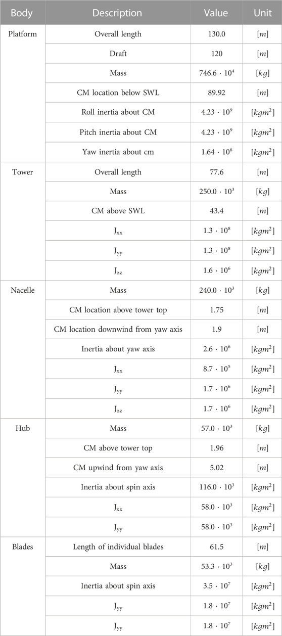
TABLE 2. Structural data Jonkman (2010).

2.11 Traditional methods of validation

Currently, tools such as Bladed by DNV, SIMO/RIFLEX by Marintek, HAWC2 by DTU and FAST by NREL are used to analyze and validate FOWT design Robertson et al. (2014); Cordle and Jonkman (2011); dnv (2023); Jonkman et al. (2010). These are fully coupled dynamic tools which account for hydrodynamic and areodynamic loads, structural dynamics, mooring and control systems in their prediction of the system response. These methods are known as the aero-hydro-elastic-servo fully-coupled approach Cruz and Atcheson (2016) and while accurate in their predictions can be time-consuming to use El Beshbichi et al. (2021b). These methods also assume a generic FOWT design which limit their usability in exploration of new design which differs significantly from the traditional FOWT.

3 Results

To facilitate comparison between existing validated work, this section will present some of the results from individual load cases. A brief overview of the load cases can be seen in Table 3 The response of the FOWT for free decay surge and pitch (Load Case 1.4 El Beshbichi et al. (2021a)) scenario as well as irregular wind and wave response [Load Case 5.2 El Beshbichi et al. (2021b)].

TABLE 3

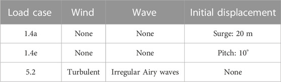
TABLE 3. Load cases, based on El Beshbichi et al. (2021b).

3.1 Free decay surge

The platform is initially displaced 20 m in the surge direction. It is released and the response is simulated accounting for hydrostatic, mooring, drag and damping loads. The results that are presented shows the response of the platform in the surge (Figure 2) and pitch (Figure 3) direction. The results show good correlation with previous findings but there are discrepancies in the amplitude and natural period due to the simplified loads which are applied in these simulations.

FIGURE 2

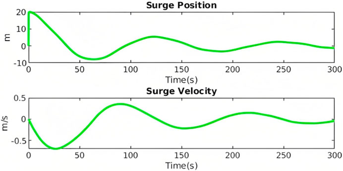
FIGURE 2. Surge response of the FOWT from Free Decay Surge.

FIGURE 3

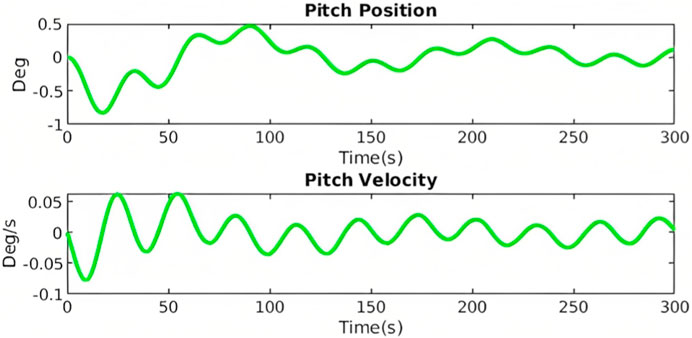
FIGURE 3. Pitch response of the FOWT from Free Decay Surge.

3.2 Free decay pitch

The platform is tilted to 10° in the pitch direction. It is also translated such that the sea-water line is not displaced in the surge direction. The results presented show the response in the surge direction (Figure 4) and pitch direction (Figure 5). As in the previous section the results are not an exact replica but correlate in orders of magnitude and frequency. The differences are readily explained by the simplified implementation of loads.

FIGURE 4

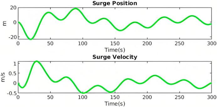
FIGURE 4. Surge response of the FOWT from Free Decay Pitch.

FIGURE 5

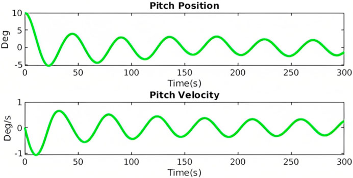
FIGURE 5. Pitch response of the FOWT from Free Decay Pitch.

3.3 Irregular wave

For this load case an irregular wave spectra with significant wave height of 6m and peak spectral period is 10s. A turbulent wind field is also created with a mean wind speed of 10m/s. Below the response in the surge direction (Figure 6), pitch direction (Figure 7) and the yaw direction (Figure 8) which is induced from the gyroscopic effect of the pitching FOWT as the rotor spins.

FIGURE 6

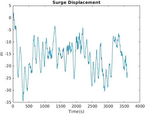
FIGURE 6. Surge response of the FOWT LC5.3 El Beshbichi et al. (2021a).

FIGURE 7

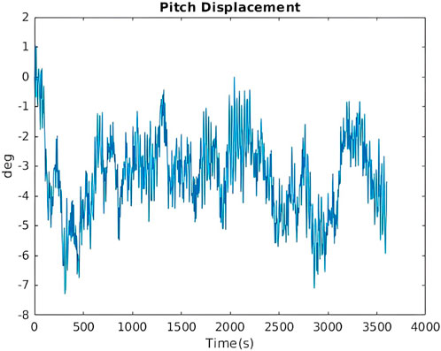
FIGURE 7. Pitch response of the FOWT LC5.3 El Beshbichi et al. (2021b).

FIGURE 8

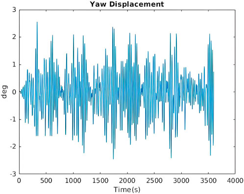
FIGURE 8. Yaw response of the FOWT LC5.3 El Beshbichi et al. (2021a).

4 Discussion

The animation is presented on this web site: https://olemg.github.io/FinalSim/. The reader is free to download the Matlab code to reproduce the results.

This project deployed the MFM to analyze the dynamic response of a floating wind turbine. This work has demonstrated how equations of motion for the analysis are easily obtained with the MFM, and in a form suitable for numerical solution by standard numerical methods. The focus of this project was not a more advanced and detailed analysis, but a validation of previous work, with a method that is more easily deployed. Using the MFM, analysts need not turn to commercial software and potential “black box” functions, but are able to create the entire software system themselves.

The results were compared to previous work done on the same FOWT El Beshbichi et al. (2021b). Figure 9 shows some of the free decay results which were found in El Beshbichi et al. (2021a). The discrepancies between this analysis and previous work are relatively simple and readily explained. The obstacles were the wave radiation, damping coefficients and related issues on the location of the center of mass. Seeing as these variables were not properly adjusted to fit this simulation results that where similar in order of magnitude and frequency were deemed sufficient. These issues do not detract from the mathematical simplicity of the MFM, nor its power.

FIGURE 9

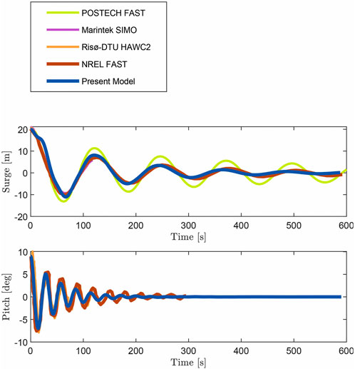
FIGURE 9. Free decay response taken from El Beshbichi et al. (2021b). “Present Model” refers to the model in that article. The heave response in the figure was removed. Licensed under CC by 4.0 (https://creativecommons.org/licenses/by/4.0/).

A validation must be conducted on the best way to solve the wave radiation damping state-space model and make it account for all couplings in all DOF’s. It could also be of interest to use the MFM to model the delta connection (crowfoot) of the mooring lines correctly such that there is no need for the added yaw spring stiffness.

The discrepancies are easy to overcome with greater attention paid to damping factors by a specialist in fluid mechanics. The primary goal of this project was to demonstrate the MFM and to create the overarching model so that such more refined analyses can be conducted. By revisiting the hydrodynamic coefficients such as the added mass matrix, damping matrix and this analysis could be more accurate (or, it might turn out that previous analyses could be improved; or both).

The results presented in this project do not precisely replicate what was previously found but this was expected due to the previously mentioned simplifications and assumptions (all of which can be revisited, improved, or, if found to be faulty, corrected). Damping can easily be introduced into this model. Once the form of the damping (say, due to wave viscosity) is assessed, one then adds it to the force vector, prior to multiplying by B-star to ensure that is involved as a generalized force.

However this project demonstrates that the moving frame method is capable of complex multi-body dynamic analysis.

5 Conclusion

There were two overarching facets to this work.

The first goal was to commence the construction of a software system to model the dynamics of floating wind turbines. In this regard, initial results have shown to be promising. The overall results capture the response of the floating turbine under various conditions, and they correspond to results predicted by commercial software. While there is some minimal discrepancy, the authors attribute this to an incomplete accounting of viscous effects and wave radiation. Ongoing work will rectify this in the next round.

The second goal of this work aligns with the philosophy of the American naturalist philosopher, Henry David Thoreau who opined, with concern, that “Man has become a tool of his tools.” In that spirit, this work has demonstrated that, with the Moving Frame Method, dynamical analysis is reduced to one equation that is readily implemented through a combination of a simple Runge-Kutta algorithm in a matrix-based environment. Furthermore, through WebGL and its interface, ThreeJS, the work is visualized through two-dimensional graphs, and with three-dimensional web pages (viewable on cell phones). In fact, the entire coding was conducted as a Bachelor project under the guidance of one professor who provided judicious advice on hydrodynamics, and another professor who taught the student the Moving Frame Method. In this way, future researchers need not rely on large-scale legacy software and readily implement analyses dedicated to the focus of their research.

6 Future work

For one of the authors, the future work consists of the dissemination of the MFM in the undergraduate curriculum. The undergraduate discipline of dynamics has become corrupted. There is, today, too heavy a reliance on the inertial frame, too much of a focus on 2D planar dynamics, and an ill-thought use of energy principles. Thus, students never learn the nuances and beauty of the discipline when focused on planar problems. Some schools split the assorted topics into other courses, further disintegrating the discipline, undermining a complete understanding, and giving rise to the disengagement many students now feel. The MFM brings reason and simplicity to dynamics, while uplifting it to three dimensions and solving advanced 3D problems at the undergraduate level. It leverages energy principles not as back-of-envelope confirmation of solutions in 2D (as is done in most textbooks today), but in its rightful place: Hamilton’s Principle and variational calculus. This coming fall, the method will be taught in three universities. The author invites any reader interested in this method to contact him to discuss access to all pedagogical content.

Data availability statement

The raw data supporting the conclusion of this article will be made available by the authors, without undue reservation.

Author contributions

YX guided on the hydrodynamic, wind and mooring loads. TI guided on the Moving Frame Method. O-MG developed the code. All authors contributed to the article and approved the submitted version.

Conflict of interest

The authors declare that the research was conducted in the absence of any commercial or financial relationships that could be construed as a potential conflict of interest.

Publisher’s note

All claims expressed in this article are solely those of the authors and do not necessarily represent those of their affiliated organizations, or those of the publisher, the editors and the reviewers. Any product that may be evaluated in this article, or claim that may be made by its manufacturer, is not guaranteed or endorsed by the publisher.

References

Austefjord, K., Hestvik, M., Larsen, L.-K., and Impelluso, T. (2018). Modelling subsea rov motion using the moving frame method. Int. J. Dynam. Control 7. V04AT06A010. doi:10.1115/IMECE2018-86191

CrossRef Full Text | Google Scholar

Burton, T., Jenkins, N., Bossanyi, E., Sharpe, D., and Graham, M. (2011). Wind energy handbook. 3. New Jersey, United States: John Wiley & Sons.

Google Scholar

Cartan, E. (1986). “On manifolds with an affine connection and the theory of general relativity,” in Monographs and textbooks in physical science (Bibliopolis).

Google Scholar

Cordle, A., and Jonkman, J. (2011). “State-of-the-art in floating wind turbine design tools,” in Proceedings of the International Offshore and Polar Engineering Conference, Beijing, China, June 20-25, 2010.

Google Scholar

Cruz, J., and Atcheson, M. (2016). Floating offshore wind energy: The next generation of wind energy. Cham: Springer Science & Business Media. doi:10.1007/978-3-319-29398-1

CrossRef Full Text | Google Scholar

DNV G1 (2023). enWind turbine design software | Bladed. Norway: DNV.

Google Scholar

Eia, M. E., Vigre, E. M., and Rykkje, T. R. (2019). “Modeling a Knuckle-Boom crane control to reduce pendulum motion using the moving frame method,” in ASME International Mechanical Engineering Congress and Exposition. Available at: https://asmedigitalcollection.asme.org/IMECE/proceedings-pdf/IMECE2019/59414/V004T05A069/6512768/v004t05a069-imece2019-10436.pdf.

CrossRef Full Text | Google Scholar

El Beshbichi, O., Xing, Y., and Ong, M. C. (2021a). An object-oriented method for fully coupled analysis of floating offshore wind turbines through mapping of aerodynamic coefficients. Mar. Struct. 78, 102979. doi:10.1016/j.marstruc.2021.102979

CrossRef Full Text | Google Scholar

El Beshbichi, O., Xing, Y., and Ong, M. C. (2021b). An object-oriented method for fully coupled analysis of floating offshore wind turbines through mapping of aerodynamic coefficients. Mar. Struct. 78, 102979. doi:10.1016/j.marstruc.2021.102979

CrossRef Full Text | Google Scholar

Faltinsen, O. M. (1990). “Sea loads on ships and offshore structures,” in Cambridge ocean technology series (Cambridge: Cambridge University Press).

Google Scholar

Flatlandsmo, J., Smith, T., Halvorsen, r. O., and Impelluso, T. J. (2019). Modeling stabilization of crane-induced ship motion with gyroscopic control using the moving frame method. J. Comput. Nonlinear Dyn. 14. doi:10.1115/1.4042323

CrossRef Full Text | Google Scholar

Frankel, T. (2011). The geometry of physics: An introduction. Cambridge: Cambridge University Press. Google-Books-ID: gXvHCiUlCgUC.

Google Scholar

Grindheim, O.-M. R. (2022). Dynamic analysis of a multi-body floating wind turbine. Shock Vib. 2022. doi:10.1155/2022/6883663

CrossRef Full Text | Google Scholar

Holm, D. (2008). Geometric mechanics, part ii: Rotating, translating and rolling. Singapore: World Scientific Publishing Company. doi:10.1142/P549

CrossRef Full Text | Google Scholar

Impelluso, T. (2017). The moving frame method in dynamics: reforming a curriculum and assessment. Int. J. Mech. Eng. Educ. 46, 158–191. doi:10.1177/0306419017730633

CrossRef Full Text | Google Scholar

Jonkman, J. (2010). “Definition of the floating system for phase IV of OC3,”. Report No:NREL/TP-500-47535. doi:10.2172/979456

CrossRef Full Text | Google Scholar

Jonkman, J. M. (2007). Dynamics modeling and loads analysis of an offshore floating wind turbine. Report No:NREL/TP-500-41958. doi:10.2172/921803

CrossRef Full Text | Google Scholar

Jonkman, J. M., Larsen, T. J., Hansen, A. D., Nygaard, T. A., Maus, K., Karimirad, M., et al. (2010). “Offshore code comparison collaboration within iea wind task 23: phase iv results regarding floating wind turbine modeling,”. Report No: NREL/TP-5000-48191. doi:10.13140/2.1.3576.5768

CrossRef Full Text | Google Scholar

Korsvik, H. B., Rognsvaag, E. S., Tomren, T. H., Nyland, J. F., and Impelluso, T. J. (2019). Dual gyroscope wave energy converter. Energy ASME Int. Mech. Eng. Congr. Expo. 6. doi:10.1115/IMECE2019-10266.V006T06A008

CrossRef Full Text | Google Scholar

Murakami, H. (2013). “A moving frame method for multi-body dynamics,” in Proceedings of the ASME 2013 International Mechanical Engineering Congress and Exposition, San Diego, California, November 15–21, 2013. In IMECE2013.

CrossRef Full Text | Google Scholar

Ogilvie, T. F. (1964). Recent progress toward the understanding and prediction of ship motions. Delft, Netherlands: The Delft University of Technology.

Google Scholar

Perez, T., and Fossen, T. (2007). “Tutorial on modelling and simulation of marine system dynamics,” in IFAC Conference on Control Applications in Marine Systems (CAMS), Trondheim, Norway, September 13-16, 2016.

Google Scholar

Robertson, A., Jonkman, J., Vorpahl, F., Popko, W., Qvist, J., Frøyd, L., et al. (2014). Offshore code comparison collaboration ContinuationWithin IEAWind task 30: phase ii results regarding a floating semisubmersible wind system. Ocean Renew. Energy Int. Conf. Offshore Mech. Arct. Eng. 9. doi:10.1115/OMAE2014-24040.V09BT09A012

CrossRef Full Text | Google Scholar

Rykkje, T. R., Leinebø, D., Bergaas, E. S., Skjelde, A., and Impelluso, T. J. (2021). Modeling friction in robotic systems using the moving frame method in dynamics. Int. J. Mech. Eng. Educ. 49, 25–59. doi:10.1177/0306419019844160

CrossRef Full Text | Google Scholar

Storaas, T., Virkesdal, K., Brekke, G., Rykkje, T., and Impelluso, T. (2019). “Stabilizing ship motion with a dual system inertial disk,” in ASME 2019 International Mechanical Engineering Congress and Exposition, Salt Lake City, Utah, November 11–14, 2019.

CrossRef Full Text | Google Scholar

Wittenburg, J. (2007). Dynamics of multibody systems. Cham: Springer Berlin Heidelberg.

Google Scholar

WWF (2022). Vindkraft og naturen.

Google Scholar