Extraction of exact symbolic stationary probability formulas for Markov chains in finite space with application to production lines. part II: unveiling accurate formulas for very short serial production lines without buffers (three- and four-stations)

Introduction: Over the past seven decades, a significant volume of research has been dedicated to manufacturing systems due to their importance in the worldwide economy. Much of this research has focused on using Markov stochastic modeling to formulate manufacturing systems problems. During the research effort, numerous numerical methods have been developed for solving such systems; however, relatively few formulas have been proposed. That is because even small systems are characterized by the well-known state explosion problem.

Methods: In short serial production lines, the underlying Markov chain is depicted as a graph of the transition diagram, which is constructed by implementing an algorithm. The steady-state probabilities are extracted in the symbolic form of two polynomial ratios. That is accomplished by employing a recently introduced method that assigns probabilities in symbolic form on the graph anti-arborescences. Finally, the performance metrics of the short production line can be obtained in exact closed-form expressions via its known definition from extant literature using straightforward algebraic operations.

Results: The closed-form formulae for the performance metrics of short serial production lines (e.g., throughput, maximum utilization, work in process, blocking probability for the second station, probability of the third station being idle, etc.) with two, three, and four stages, absent buffers, are presented herein for the first time in the extant literature. The proposed algorithm results shed light on the well-known phenomenon of production lines known as the “bowl phenomenon”. Comprehending the formula structure enables the formulation of a straightforward model for throughput estimation for fully balanced short serial production lines using genetic programming for lines up to thirteen stages.

Discussion: The enormous size of the exact formulas highlights the need for more computational support for production lines larger than four stages without buffers. A comprehensive understanding of the underlying principles governing exact formulas will facilitate the implementation of innovative mathematical approaches to problem-solving. This understanding will also enable artificial intelligence to derive precise mathematical relationships with reduced complexity, thereby fostering intuition in production lines.

1 Introduction

A significant part of the world’s economic progress and development after 1950 was based on manufacturing, where specialization and the sharing of labor and resources led to the growth of production lines. One consequence of the invention of the assembly line was the scientific research that followed, leading to the development of manufacturing systems in Industry 4.0. Areas such as empirical studies, modeling, analysis, design, control, optimization, and monitoring have become a fundamental part of manufacturing research for seven decades, along with computing and operational research advances. Thus, numerous scientific studies, papers, monographs, and books have been devoted to the problems and issues of manufacturing systems. All these works aim to improve the efficiency of production lines by estimating their productivity. Many performance metrics are of interest, but the most valuable insights for a production line come from evaluating its average throughput, i.e., the average number of finished parts produced in the long term by the last machine of the system per unit of time (Papadopoulos, 1996).

The efficient solution of production lines is a complex and challenging task due to their configuration into composite topologies and their size, which lead to internal interactions between the line components, increasing the variability due to stochastic factors. The modeling of production lines as a Markov process aims to analyze the stochastic behavior of production lines and to serve as a tool for their performance estimation. However, these systems’ complexity prevents a broader development of exact methods, i.e., closed formulas that express the throughput symbolically and error-free or numerical methods whose only flaw is the inaccuracy of digital computers.

The exact closed formulas are too few and refer to the throughput and maximum utilization for short serial production lines without intermediate buffers of two and three stages presented in Hunt’s work (Hunt, 1956). Since then, considerable efforts have been made, and remarkable results have been achieved in many aspects of production line problems. Still, the development of closed formulas was not one of them due to the combinatorial explosion.

In this work, we use the results of the work presented in the paper (Boulas et al., 2024a) to obtain not only the throughput but all performance measures for short serial production lines for two to four stages without intermediate buffers. It is shown that the size of these formulas increases exponentially. Thus, the reasons that prevent the scientific community from developing closed formulas are explained, and it becomes understandable why scientific research could not go beyond Hunt’s work for almost seven decades.

The rest of the paper is organized as follows. Section 2 reviews the literature, focusing primarily on the formulae literature for evaluating the performance of production lines. The production line model and its assumptions followed by the Algorithm (With capitalized A refers to the Algorithm proposed in this work), which constructs the transition state diagram for short serial production lines under the model assumption, are presented in Section 3. The exact results of the formulas for K = 2,3,4 stages and the complexity for longer stages, the well-known bowl phenomenon by the aspect of spanning trees, and a simple formula produced by Genetic Programming are presented in Section 4. This is followed by the Discussion, Summary, and Conclusion sections, which include further research in Sections 5, 6, respectively.

2 Review of the literature on the performance evaluation of production lines

The literature on production systems presents a detailed study of developing methods for evaluating the performance of production lines. The extensive reviews summarize the primary research; further details can be found in the comprehensive reviews by Buzacott and Shanthikumar (1992) and by Dallery and Gershwin (1992). The book (Buzacott and Shanthikumar, 1993) provides a general description of production line performance measurement.

2.1 The use of markovian analysis and numerical methods for performance measurement

Research publications on estimating performance measures using formulas are dominated by throughput estimation formulas based on empirical studies, simulations, or Markovian analysis. Most Markovian analysis studies assume processing times that follow exponential or phase-type distributions (Papadopoulos et al., 2019). The steady-state probabilities of these systems are determined by solving linear systems of equations, as in the work of Hunt and Hatcher (Hunt, 1956; Hatcher, 1969), in which they analytically solved the system models under investigation. Works in which the linear systems of equations are solved numerically include the work of Hillier and Boling (Hillier and Boling, 1966; Hillier and Boling, 1967). The main problem of Markovian analysis is the vast state space, see Papadopoulos et al. (1990), which overgrows and becomes an obstacle to implementing the method. However, various studies have significantly contributed to developing methods for evaluating production lines, making significant progress and evolution in the field.

The complexity problem leaves a more significant footprint when developing formulas for expressing performance measures. The exact solution of a system longer than 13 stages requires sophisticated techniques such as Stochastic Automata Networks (SAN) (see Fernandes et al., 2013b; Fernandes et al., 2013a). Although numerical methods have been used to obtain exact solutions for up to 13 stages using the MARKOV algorithm, see the book by Papadopoulos et al. (2009), there are no exact closed-form formulas of throughput for lines longer than three stages.

The book by Ghezzi et al. (2017) provides an account of the changes that Industry 4.0 will bring to production systems. It introduces the new concepts of production through a series of examples of production systems and discusses the essential role of mathematics in the competitiveness of manufacturing companies and the most advanced mathematical models and simulation tools for production optimization. But the role of human intuition despite technological advancement is explored in Gershwin (2018), where the human factor plays a central role in the design of high-performance production systems. The paper shows how analytical models enhance human intuition and help to achieve optimal solutions. The human factor is discussed in Cañas et al. (2021), where a classification of the principles of Industry 4.0 design is made, taking into account a series of classification aspects. It also analyzes a series of conceptual frameworks of reference that deal with the definition of term Industry 4.0.

2.2 Literature about formulas for throughput estimation

Hunt, with his early work (Hunt, 1956) was the first to analyze production lines with two and three stages without buffers, among other cases of production line configurations, assuming processing times that follow exponential distributions. He solved the system of differential equations and obtained solutions in the form of a ratio of two polynomials. The solutions were close to the maximum utilization; thus, the exact throughput estimate of the Markov process was obtained. Hunt’s model was slightly different because the arrival of the workpieces at the front of the production line under study was subject to a Poisson distribution. Hunt’s formula for the three stages is very significant as it implicitly limits the size of the system under study due to the complexity of the exact formulas (Muth, 1984).

Hunt’s work motivated other researchers to address the problem of throughput estimation, such as Hillier and Boling (Hillier and Boling, 1967), who developed a method for the exact solution of a short serial production line without buffers. This work also creates an approximate recursive formula for longer lines and exponential processing times, which is solved using numerical methods. In Haydon (1973) and Scale (1972), the authors used approximate solutions in their dissertations. They established approximate formulas for the throughput of flow or production lines. Using the concept of the “cyclic queue,” a simplified formula for exponential service times was developed by Basu (1977) to optimize buffer capacity given three cost parameters. A prediction formula for the throughput of K-stage production lines based on empirical results of other studies was presented by Panwalkar and Smith (1979).

Muth introduced the stochastic model of the holding time to analyze production lines (Muth, 1977; Muth, 1984). The method can quantify the times taken by successive orders at each workstation on the line by using integral equations. Both exponentially and generally distributed processing times can be analyzed. The author mentioned Hunt’s work at length and made a critical observation (Muth, 1984, p. 65) of the paper: “It should be noted that the state-transition rate diagram of an ergodic Markov process is implicitly a representation of the equations defining the equilibrium conditions.” For the case of three non-identical stations based on service times with exponential distributions and two-station Erlang distributions, the author derived a simple analytical formula for the throughput. It was assumed that the service time at each workstation follows a different stochastic process. Muth’s work provided closed-form solutions for three non-identical exponential stations and two Erlang stations. Although the result for exponential servers is identical to Hunt’s, it is characterized by a much simpler structure since it is a sum of simple fractions rather than a ratio of two polynomials. Muth and Alkaff extracted a general throughput estimation formula using the first station’s holding time (Muth and Alkaff, 1987). The authors solved the problem of a production line with three stations if the service times of stations one and three follow phase-type distributions. Still, the service time of station two follows a Laplace-transformable distribution. Muth studied asynchronous production lines with K-serial workstations (Muth, 1987), where he analyzed transfer lines with stochastic service times subject to failure and repair with no intermediate buffer between two consecutive stations. The author solved the model using a combination of theory and numerical curve fitting to extract the throughput formula. Alkaff and Muth (1987) extended the analysis of Muth’s holding time model (HTM) to longer production lines, establishing exact throughput formulas for a balanced line. The holding time concept of Muth’s method was also used in the work of Rao (Rao, 1975a; Rao, 1975b; Rao, 1976a; Rao, 1976b), where integral equations were used to deal with specific problems of production lines.

Mishra et al. (1985) determined two closed-form formulas for the throughput of production lines with three stations, in which the processing time of the first and third stations was exponentially distributed. In contrast, the processing time of the second station followed either a gamma or a hyper-exponential distribution. In Hira and Pandey (1987) and Dar-El and Mazer (1989), multiple regression was used to derive analytical mathematical formulas. Blumenfeld extended Muth’s formula (Blumenfeld, 1990) to approximate the throughput between two consecutive workstations of the production line by introducing the buffer size as a parameter. The proposed simple formula for throughput was a function of four parameters: mean and standard deviation of service or processing times, number of stations, and buffer size. Martin (1993) investigated the problem of accurately predicting the efficiency of a production line with an arbitrary number of workstations and intermediate buffer capacities. The author assumed realistic distributions of processing times. In Baker et al. (1994), a line with three workstations and no intermediate buffers was analyzed to obtain an approximation of throughput. The authors developed a set of simple predictors using simple cases of a general line to feed an algorithm for the general case. Their methods utilized the exponential case for which exact throughput values were known. In addition, the authors tested their results using simulated data for two classes of uniform distributions and a lognormal distribution. The holding time model (HTM) was also used to calculate the throughput of a K-station production line in Papadopoulos (1996). Throughput was derived as an approximate analytical formula for workstations with different mean processing times. Also, a formula for the case of the balanced lines was proposed. A formula for lines with identical workstations subject to random failures and intermediate buffers of equal size between workstations was obtained by Blumenfeld and Li (2005). In Dhouib et al. (2010), the authors proposed an analytical model to assess the variance of the throughput of homogeneous transfer lines with no intermediate buffers. Their model allowed machines to break down, whereas service and repair times were assumed to follow the exponential distribution.

Unpaced serial production lines with parallel machines at each workstation were investigated by Magazine and Stecke (1996) to improve performance. The authors gave the results of their formula by a series of curves. Based on the decomposition method, see Gershwin (1987), two analytical formulas for estimating the throughput of a reliable production line with exponential service times and finite intermediate buffers were developed by Li et al. (2016). The case of a nearly balanced line with identical buffers or almost optimal buffer allocations was investigated.

The problem of calculating throughput in a serial production line is of considerable interest due to its impact on the cost of the production process. In (Aboutaleb et al., 2017) an independent closed-form formula for the throughput rate of normally distributed asynchronous human-dependent serial flow lines was derived using data mining and simulation modeling. In Bai et al. (2021), a new aggregation-based iterative algorithm is proposed to compute the performance metrics of a serial line with multiple machines by representing it as a set of virtual lines with two machines. Energy consumption is also of great interest. A Markov chain model is set up to interpret the dynamics of serial production lines with N-policy. The analytical formulas for production rate and energy consumption are derived in Cui et al. (2021). An energy-efficient control model is then formulated to establish a balance between productivity and energy consumption.

In the work (Magnanini and Tolio, 2023), a novel analytical model for the performance evaluation of asynchronous, unreliable production lines for manufacturing discrete parts with finite buffers and deterministic processing times is presented. This approach is based on continuous-time Markov chains with continuous flow. The same work recognizes that performance evaluation models become relevant as evaluation kernels within decision support tools that can be used as synthetic, computationally effective models of the entire multilevel system.

2.3 The use of intelligent techniques and graph theory for obtaining throughput formulas

The complexity of production systems makes it attractive to use artificial intelligence to address a variety of problems in the production process. A number of different aspects of the problem are presented in (Kang and Bhatti, 2019; Arinez et al., 2020; Sankhye and Hu, 2020; Ayvaz and Alpay, 2021; Subramaniyan et al., 2021; Fragapane et al., 2022; Alkhalefah et al., 2023).

Symbolic regression is a method for obtaining formulas that describe underlying processes using a set of values of independent variables and their corresponding dependent variables. An essential evolutionary technique for symbolic regression tasks is genetic programming (GP) (Koza, 1992), which is classified as artificial intelligence. A number of attempts to express throughput have been made using GP and comparisons have been made with other techniques showing the effectiveness of the method (Can and Heavey, 2009; Can and Heavey, 2011; Can and Heavey, 2012).

In Papadopoulos et al. (2002) genetic programming was used, along with decomposition techniques, to obtain throughput formulas for short production lines with two, three, and four machines and buffers.

The same evolutionary technique was used to obtain a set of approximate formulas for throughput presented in the work by Boulas et al. (2015), Boulas et al. (2017) by using DECO-2 and MARKOV algorithms, see Papadopoulos et al. (2009) to build training sets for GP. The same team found that satisfactory approximate solutions with high accuracy can eventually be expressed as a two-polynomial ratio. Boulas et al. (2018) extended this observation for the studied case of two workstations with parallel machines. The training set was formed using the DECO-2 algorithm, which provides the exact results for this production line type. Finally, the GP results presented in Boulas et al. (2018) can be expressed in a two-polynomial relation. Thus, a hybrid Genetic Programming (GP) and Genetic Algorithm (GA) scheme (Holland, 1992) was proposed by Boulas et al. (2021), which can obtain efficient formulas as a ratio of two polynomials with integer coefficients and exponents, like Hunt’s formulas.

The same team developed a method to symbolically represent a Markov chain’s stationary probabilities, given in Part I of this work (Boulas et al., 2024a). With its practical application, this method creates a probability space. It extracts all probabilities consistently using the set of anti-arborescences of the state transition diagram, thereby enhancing the usability of the research findings. In order to obtain the exact formulas for the performance measurement of a K-stage production line, a crucial step involves constructing the graph representing the state transition rate diagram using an appropriate method. Subsequently, the symbolic steady-state probabilities are extracted from the anti-arborescences, following the procedure developed in Part I, (Boulas et al., 2024a). Each anti-arborescence represents a product of mean service rates that forms a monomial. The sum of the monomials of a given graph vertex anti-arborescence (or a system state) forms a polynomial. The latter, divided by the sum of all polynomials of all graph vertices, is the steady-state probability of the specific system state. The system performance estimation is then reduced to algebraic operations of polynomial ratios for each stationary probability available by the method presented in Part I of this work (Boulas et al., 2024a), thereby providing a clear understanding of the research methodology.

3 Applying the methodology to extract formulas using the underlying graphs representing short serial production lines

The production lines are complex and contain various topologies to produce goods economically. On the way of the product within the production line, there are branches and connections or loops, parallel machines, control and inspection stations, and processing and assembly or disassembly operations. In addition, in practice, machines are always broken down. Even the size of the lines varies, reaching a few hundred stations in industries such as automotive. The flow of workpieces is carried out to increase the added value, and the final products are their result. This work uses a simplified model to study short serial production lines without intermediate buffers between workstations. This type of production line is simple to model but challenging to operate because the absence of intermediate buffers leads to the vital phenomena of blocking and starving, which increases variability and reduces line throughput. This production line type is the fundamental structural unit for understanding the deeper mechanisms governing these complex production lines.

3.1 The model of operation of the short serial production lines

The assumptions of the model considered in this paper are given below. For simplicity, we assume reliable workstations with individual machines per workstation and the service or processing times to be stochastic, following the negative exponential distribution.

Figure 1 shows a production line with single machine workstations indicated by the rectangles M_i, i = 1,2, … , K. The jobs enter the production line from the first workstation via a warehouse with an unlimited capacity of raw products. They are routed sequentially from the first to the last workstation, M_K. The K machines pick the workpieces sequentially, with one machine per stage. When the parts have completed their processing on each machine, they move on to the next one until they become finished products. Each machine state can be characterized as 0: idle, 1: working, and 2: blocked. The system’s state consists of three digits, i.e., the composition of the states of the individual machines following the above indicators. When processing is complete, they leave the system and are placed in a warehouse with unlimited capacity. The assumptions of the model considered in this study are similar to those in (Papadopoulos et al., 2009), which are summarized below.

1. The first warehouse, W_in, is assumed to have an infinite capacity of raw parts to supply the first station, which is never starved. That is called a saturated production line.

2. The last station, M_K, is assumed to be never blocked, i.e., it is assumed that there is enough space in the warehouse after the last machine to accommodate the finished products.

3. It is assumed that all machines’ processing or service times follow the negative exponential distribution with mean service rates μ_i (i = 1, 2, … , K), which are generally not identical.

4. The machines are assumed to be perfectly reliable, i.e., never fail.

5. There are no intermediate buffers between the workstations.

6. The line is subject to the so-called blocking phenomenon. When machine M_j has finished processing, and there is a part in the downstream machine M_j+1, machine M_j cannot start processing the next job because it is unavailable. So, machine M_j blocks the processing of the following job until the next downstream machine is empty.

Figure 1

Figure 1. A K-station production line with K single-machine stations and two warehouses of infinite capacity in front of the first station and after the last station.

The model described above was chosen for its simplicity. There are algorithms to calculate the exact throughput of these simple systems numerically. One of these, called MARKOV, was developed by Heavey (see the papers by Papadopoulos, Heavey, and O'Kelly (Papadopoulos et al., 1989; Papadopoulos et al., 1990) and Heavey, Papadopoulos, and Browne (Heavey et al., 1993)). The MARKOV algorithm is available in the book Papadopoulos et al. (2009). A similar algorithm was proposed by Hillier and Boling (1967).

The above model ensures that the operation of the production line can be modeled as a Markovian chain. The rate transition matrix Q with the elements of transition rates from state i to state j, q_ij, is a powerful tool for solving such systems to determine the vector of stationary probabilities, π, from the solution of the Equation π·Q = 0, (Gershwin, 1994; Altiok, 1997; Papadopoulos et al., 2009). Once the vector of steady-state probabilities π has been extracted, it is easy to obtain the system performance measures. For example, the maximum utilization, ρ_max, can be defined as the sum of stationary probabilities at which the first workstation in the line is not blocked. The estimate of throughput is obtained as the numerical product of the first machine’s service rate μ₁ multiplied by the maximum utilization rate, i.e., X = μ₁·ρ_max. The work in process, $\overline{WIP,}$ of the system is the internal product of the incomplete parts in the production line for every system state E, multiplied by the vector of stationary probabilities π, $\overline{WIP}=\mathit{\pi }·\mathit{E}$. One can extract many other performance measures of interest using the stationary probabilities vector. One example is the probability that the second machine is blocked, Bl₂. It is the stationary probability for which $\mathit{Pr}\left(M_2^{Bl}\right)=B{l}_2={\sum }_{i,where{M}_2=2}{\pi }_i$, Moreover, the list continues for each performance measure considered.

The ability to express the stationary probabilities accurately in analytic form is the intermediate stage in developing the exact formulas for evaluating the efficiency of the production lines. The main objective of our study is to develop a set of formulas for estimating the exact solutions for each performance measure of short serial production lines with K = 2, 3, 4. The complexity of the problem prevents further extraction of formulas for the case of 5 stations since the combinatorial explosion leads to an enormous solution size of the exact formulas, which is very difficult to obtain or even to represent.

3.2 The algorithm that constructs the graph for short serial production lines without buffers

For the numerical solution of the production lines, it is crucial to form the transition rate matrix Q (Papadopoulos and O'Kelly, 1993; Papadopoulos et al., 2009). In our case, where we solve the system analytically, the transition rate diagram between the system states may be formed instead of obtaining the anti-arborescences following the Algorithm presented in Part I of this work (Boulas et al., 2024a). That task, specifically for production lines without buffers, is done using the Algorithm of the present work, see Table 1. The Algorithm, consisting of the steps given below, forms the transition graph that determines the transition between an initial and a final state weighted by the mean service rate of the machine that causes this transition after the completion of the processing of a workpiece. Τhe methodology for solving small serial production lines can be summarized in the following three basic steps, which are briefly explained to understand the general application of the solution approach.

Step 1: Definition of the system to be solved (number of stations K).

Step 2: Determination of the graph describing the underlying Markovian chain of the system. In this Step, a graph from any source can be used. In this work, the Algorithm is used. However, the graph can be manually inserted into the Algorithm given in (Boulas et al., 2024a) to extract the exact stationary probabilities. The graph defines the system to be solved. For example, serial production lines with buffers and parallel machines per workstation are distinguished by the different graphs that describe those systems.

Step 3: The Algorithm presented in (Boulas et al., 2024a) is executed. This algorithm forms and assigns the stationary probabilities in analytic form based on the transition weights between the nodes of the graph w(u, v). The Algorithm forms the spanning monomials, spanning polynomials, and, finally, the ratios of the stationary probabilities.

Table 1

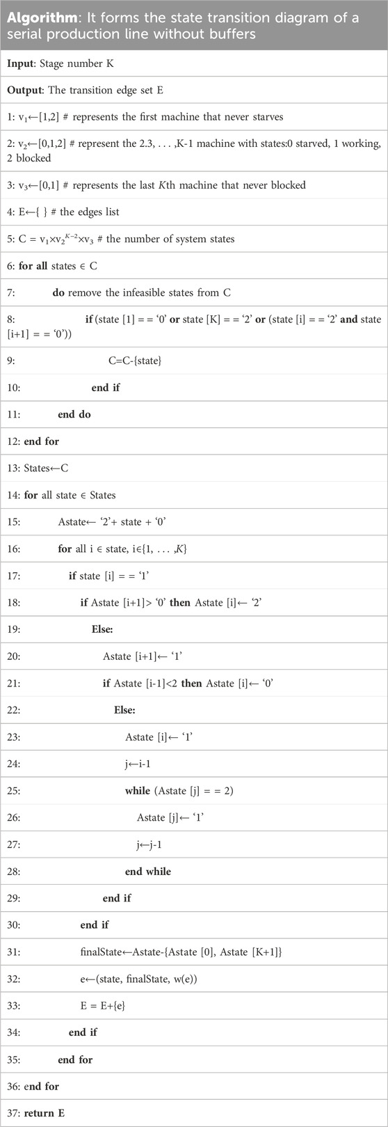
Table 1. The algorithm that forms the state transition diagram.

The Algorithm’s logic is to generate all feasible states of the system under consideration and then generate all transitions to a feasible final state for each initial feasible state. The transition from one initial state to another final state will be based on the mean service rate of a machine operating in the initial state according to the model’s assumptions. That mean service rate will be the weight of the graph’s edge for the transition from the initial to the final state. An initial state will have as many final states as the number of machines working. That is, for a system with four machines and a state of 1011, we will expect three final states of 1111, 1021, and 1010 depending on the order of completion of machining on each machine, i.e., first, third, and fourth machines, respectively.

The Algorithm receives the stage number K of the production line as an argument and forms the transition graph as an edge list, E. Each edge of the transition graph includes the initial state, the final state, and the weight of the edge, i.e., the mean service rate of the corresponding machine that causes the transition from one state to another, according to the assumed model. The Algorithm uses an auxiliary state called “Astate” to handle the model workflow, which is dropped off when the final state of the transition is obtained.

Using the variables V_i, i = 1,2,3, all possible states of the machines of each workstation of the line are determined under the model assumptions. V₁ and V₃ are the possible states of the first and Kth stations, respectively, while each of the machines in the intermediate stations can assume the three possible states of variable V₂ (Steps 1–3). Since C has some infeasible system states as members, i.e., like a blocked machine followed by an idle machine, it must be freed from all these problematic states. The line 4 initializes the edge list of the graph to an empty list. The Cartesian product of line 5 contains the number of all possible states of the system and the infeasible states, which should be subtracted from the set of feasible states of the system. That is the task in the “for loop” lines 6–12, where only feasible states are kept. The final tidied set C contains all feasible system states, called States, i.e., the nodes of the transition graph, line 13.

Next, for each initial system state, we need to extract the final state where the system ends up in the considered system state after the completion of the work of each initially busy machine. That is the purpose of the “for loop” (lines 14–36), in which every feasible system state is examined. Each system state is an ordered set of elements according to the state of each machine, i.e., idle, working, and blocked. The system state has K-ordered digits, each one for the respective state of the machine. Each element represents the corresponding state of the machine, i.e., idle: 0, busy: 1, and blocked: 2. The state elements representing busy machines are interesting because they cause the transitions from one system state to another, i.e., each system state causes the same number of transitions that are equal to the number of its busy machines. The Algorithm aims to find all these elements corresponding to busy machines to detect the next system state when the considered busy machine has finished processing the workpiece.

The subsequent system state is reached via an edge (arc) with a weight equal to the mean service rate of the machine. The Algorithm uses the auxiliary state Astate, which is extended by two elements to estimate the system’s transformation. The element ‘2′at the beginning of the state simulates the infinite queue at the beginning of the production line. At the end of the state, the element ‘0′is added to represent the infinite capacity warehouse that prevents the blocking of the Kth machine, line 15. All transformations for the final state estimation occur on Astate, which has K+2 elements. The Algorithm examines only the machines that can make system transitions after finishing their work in the ‘if statement’ of line 17. When the ith machine is busy, a transition occurs, i.e., a graph edge from the initial state under consideration to a feasible final state that must be found.

In line 18, the state of the following production line machine, i.e (i+1), is considered. If it is unavailable, the workpiece blocks the ith machine until there is room to move on. If the next machine is free, the workpiece is moved there, and processing starts immediately in line 20. To get the system’s final state, it is necessary to check what happens on the upstream side of the ith machine (lines 21–29). If no workpiece is available, the ith machine enters the idle state, line 21; otherwise, the processing immediately enters the busy state, line 23, and the subsequent upstream blocked machines immediately release their parts and enter the busy state, as specified by the while loop of the Algorithm.

All these changes occur in the auxiliary system state, the Estate, from which the final system state is formed by truncating the front queue and end-of-system store states, line 31. The initial system state forms the transition edge e, the final system state, and the weight of the edge, viz., the machine’s mean service rate that finishes its job, causing the system’s transition to the next state, line 32. The transition graph is formed by an edge list summarizing all the initial state transitions, line 33. That list of edges E represents the state transition diagram, which is the result of the Algorithm and is returned at the end in line 37.

The state transition diagram in the edge list E is the input for the automatic extraction of analytic stationary probabilities of finite Markov chains using the method presented in Boulas et al. (2024a). The edge list E reverses direction, and each spanning tree rooted at each node is obtained. Reversing direction again and going along each anti-arborescence, a monomial is formed by multiplying each edge weight, i.e., mean service rate. This monomial is called a spanning monomial. The spanning monomials of all anti-arborescences ending on a given vertex v_i are summed up to form the v_i vertex spanning polynomial. $s{p}_{v_i}$. All the spanning polynomials are summed up to form the graph spanning polynomial sp_G, which normalizes all probabilities to one. The sp_G is the denominator of the stationary probabilities of each vertex, i.e., the system state. The corresponding numerator is the vertex-spanning polynomial. Since the stationary probabilities are in analytic form, the estimation of the performance measures is a matter of algebra, following the analysis mentioned above at the end of Section 3 about stationary probabilities formation.

4 Results for short serial production lines

This Section presents the results of implementing the methodology presented in Boulas et al. (2024a) of our research for lines with K = 2, 3, and four stations using the graphs constructed by the Algorithm of the present work. These results also serve as examples of how the proposed methodology works. For lines with K ≥ 5 stations, a presentation of the critical problem of the size of the exact formulas using the results of the methodology follows.

4.1 Case K = 2

The two-station production line is the most straightforward, non-trivial system of coupled machines for analysis and provides a good starting point for generalizations and the development of methods such as decomposition for performance estimation (Gershwin, 1994). Moreover, under the assumptions of the model adopted in this work, the two-station system provides an opportunity to get an overview of the solution approach for determining analytic probabilities without being burdened with all the complications of combinatorial explosion, an inherent feature for longer lines. Equation 1 shows the transition matrix Q of the system, and Figure 2A shows the associated state transition diagram with the three anti-arborescences shown in Figures 2B–D, which are easily obtained. The edge weight product, i.e., the mean service rates of the exponential distribution of each anti-arborescence, forms the corresponding spanning monomial $s{p}_{10}={\mu }_2^2,s{p}_{11}={\mu }_1·{\mu }_2,s{p}_{21}={\mu }_1^2$ for the states ‘10’, ‘11’, and ‘21’, respectively. The spanning polynomial of the graph is the sum of all monomials and is the denominator of the steady-state probability, i.e., $s{p}_G=s{p}_{10}+s{p}_{11}+s{p}_{21}={\mu }_2^2+{\mu }_1·{\mu }_2+{\mu }_1^2$. Thus, the steady-state probabilities vector $\mathit{\pi }$ is presented in Equation 2 and can be easily determined, which is the solution of the Equation $\mathit{\pi }·\mathit{Q}=\mathbf{0}$, while it holds ${\displaystyle \sum _{i\in S}}{\pi }_i=1$ where $S=\left\{10,11,21\right\}$ is the set of states.

$\mathit{Q}=\left(\begin{array}{ccc}-{\mu }_1& {\mu }_1& 0\\ {\mu }_2& -\left({\mu }_1+{\mu }_2\right)& {\mu }_1\\ 0& {\mu }_2& -{\mu }_2\end{array}\right)(1)$

$\mathit{\pi }=\left[{\pi }_{10},{\pi }_{11},{\pi }_{21}\right]=\left[\frac{s{p}_{10}}{s{p}_G},\frac{s{p}_{11}}{s{p}_G},\frac{s{p}_{21}}{s{p}_G}\right]=\left[\frac{{\mu }_2^2}{{\mu }_2^2+{\mu }_1·{\mu }_2+{\mu }_1^2},\frac{{\mu }_1·{\mu }_2}{{\mu }_2^2+{\mu }_1·{\mu }_2+{\mu }_1^2},\frac{{\mu }_1^2}{{\mu }_2^2+{\mu }_1·{\mu }_2+{\mu }_1^2}\right](2)$

Figure 2

Figure 2. The state transition diagram (A) for K = 2, and the three anti-arborescences for the states (B) “10” (C) “11”, and (D) “21”.

In his work, Hunt (Hunt, 1956) calculated the maximum utilization for two stages without buffers, ${\rho }_{\mathit{max},2}=\frac{{\mu }_2{\mu }_1+{\mu }_2^2}{{\mu }_1^2+{\mu }_1{\mu }_2+{\mu }_2^2}$. The maximum utilization is the sum of the steady-state probabilities at which the first machine in the system is not blocked, i.e., ${\rho }_{\mathit{max},2}={\pi }_{10}+{\pi }_{11}$, which amounts to the same formula as Hunt’s Equation. In the same way, it is easy to express the other performance measures using the steady-state probabilities in the analytic form of Equation 2.

4.2 Case K = 3

Hunt analyzed the case of a system with K = 3 stations without buffers (Hunt, 1956), where he gave the analytical solution for the maximum utilization and throughput by extracting the equations for the steady-state probabilities from a set of difference equations. In this work, a different approach is followed using the state transition diagram of the system and the methodology introduced in (Boulas et al., 2024a) for extracting the steady-state probabilities in the analytic form to extend Hunt’s work to other performance measures. The Algorithm obtains the state transition graph and corresponds to that presented in Muth’s work (Muth, 1984). The graph is shown in Figure 3A and Equation 3 represents the corresponding state transition matrix used to show that the analytic transition probabilities are the exact solutions of the underlying Markov chain. The graph has eight vertices and 14 edges, making it tedious to detect anti-arborescences without a computer, as in the case of K = 2 stations. Therefore, the Algorithm given in (Boulas et al., 2024a) is used to overcome this difficulty and find all 78 anti-arborescences of the graph of Figure 3A that form the corresponding monomials. The state ‘100′will be used as an example of the technique since it occurs in all production lines from K = 1 stations, i.e., the system state in which only the first machine is working and all others are idle with no workpiece in them, i.e., the states ‘1’, ‘10’,'100’, ‘1000’ and ‘10000’ for K = 1,2,3,4, and five stations, respectively. This state can be used for comparison to understand the growth of the size of the analytic steady-state probabilities. For the considered case of K = 3 stations, there are eight different and unique anti-arborescences for the ‘100’ state, which have the opposite direction, as shown in the computation tree in Figure 4. The first of the eight spanning trees is also the first of the 78 spanning trees of the whole graph, as shown in Figure 3B. On the right side of Figure 3C, the spanning tree T₁ of Figure 4 with the root in the ‘100’ state is shown, which generates the anti-arborescent from Figure 3B by reversing the edge direction. The edge direction reversal step is necessary because the Algorithm of Gabow and Myers (Gabow and Myers, 1978), a part of the methodology, can only enumerate the rooted spanning trees. If the edge direction inversion is not done, some spanning trees will not be formed appropriately, so the exact solution cannot be found.

$\mathit{Q}=\left(\begin{array}{cccccccc}-{\mu }_1& 0& {\mu }_1& 0& 0& 0& 0& 0\\ {\mu }_3& -\left({\mu }_1+{\mu }_3\right)& 0& {\mu }_1& 0& 0& 0& 0\\ 0& {\mu }_2& -\left({\mu }_1+{\mu }_2\right)& 0& 0& {\mu }_1& 0& 0\\ 0& 0& {\mu }_3& -\left({\mu }_1+{\mu }_2+{\mu }_3\right)& {\mu }_2& 0& {\mu }_1& 0\\ 0& {\mu }_3& 0& 0& -\left({\mu }_1+{\mu }_3\right)& 0& 0& {\mu }_1\\ 0& 0& 0& {\mu }_2& 0& -{\mu }_2& 0& 0\\ 0& 0& 0& 0& 0& {\mu }_3& -\left({\mu }_2+{\mu }_3\right)& {\mu }_2\\ 0& 0& 0& {\mu }_3& 0& 0& 0& -{\mu }_3\end{array}\right)(3)$

Figure 3

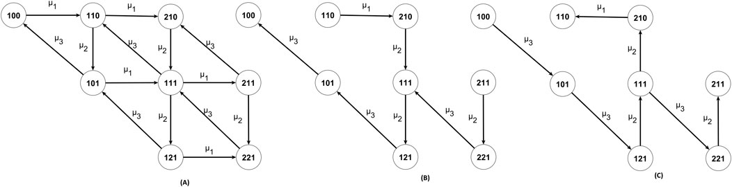
Figure 3. (A) The state transition diagram of the K = 3 stations line, (B) The first spanning tree of the graph ending in state “100”, and (C) The respective anti-arborescent rooted in state ‘100’, the equivalent of the computation tree T₁ of Figure 4.

Figure 4

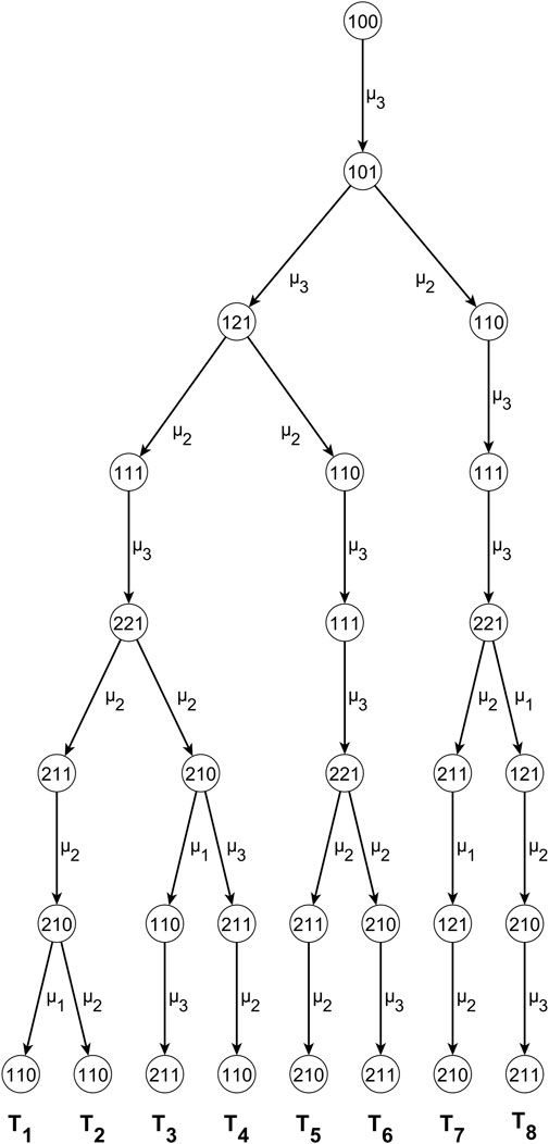
Figure 4. The computation tree of all spanning trees rooted on the state “100” for the line with K = 3 stations.

Figure 4 shows the computation tree (Gabow and Myers, 1978) for the system state ‘100'. The edges are shown in the opposite direction from the original graph, as they are intended to use Gabow and Myers’ Algorithm to generate anti-arborescences. The computation tree shows how the spanning tree T grows. The Algorithm of Gabow and Myers creates it and shows the steps to form the spanning tree. The spanning tree is uniquely extracted from the computation tree due to the simple rule that each edge added to T must start inside T and end outside of T. The spanning tree is a tree of edges and vertices. All edges and vertices belong to the graph created by the Algorithm, as shown in Figure 3A. Thus, applying the rules does not allow misleading regarding which edge is involved in each case. The spanning tree of T₁ ending in state ‘100’ is shown in Figure 3B, while the anti-arborescence rooted in state ‘100’ is shown in Figure 4C.

In Figure 4, each expansion of the subgraph Ti, i∊ {1.2,...8} is represented by a node indicating the last system state introduced into the spanning tree subgraph Ti, and an edge starting from Ti and leading to a node outside of Ti so each Ti is growing up progressively. Because of the model used, one edge can have the same weight, i.e., mean service rate, as another without confusion about which edge it is. The pair of edge and endpoint is unique in the graph and uniquely defines the spanning tree in the original direction (anti-arborescent in the reversed direction) that grows along the path indicated by the transition rate graph. The Ti grows until it encompasses all nodes of the graph node and reaches a depth equal to the number of states-1 levels (here, the states are eight, and the depth is seven). The number of levels determines the sum of the exponents of the individual monomials. When all graph nodes have been included, Ti is an anti-arborescent of the graph in the reversed direction (a spanning tree in the forward direction) and can be obtained. The recursive procedure continues until all anti-arborescences rooted in state ‘100’ have been obtained.

From the point of view of creating analytic stationary probabilities, the product of the edge weights, i.e., the mean service rates, that form the spanning monomial is of interest. For example, when analyzing the leftmost path of the computation tree (T₁), form the product and the corresponding spanning monomial as follows: ${\mu }_3·{\mu }_3·{\mu }_2·{\mu }_3·{\mu }_2·{\mu }_2·{\mu }_1={\mu }_1{\mu }_2^3{\mu }_3^3$. The sum of all spanning monomials gives the spanning polynomial of the considered state: the anti-arborescences root if the edges’ direction is reversed, or interchangeably the last vertex of the spanning trees if the edges have their original direction. For the system with K = 3 stations, the algorithmic approach introduced in (Boulas et al., 2024a) forms the spanning polynomial for each of the eight system states shown in Equations 4–11. The spanning polynomial of the entire graph is the sum of all cross-state polynomials and is the denominator of the stationary probabilities normalized to one. Equation 12 shows the spanning polynomial for the entire graph for the K = 3 stations line, and it is the same as the denominator in Hunt’s Equation for maximum utilization (Hunt, 1956).

$s{p}_{100}=2{\mu }_1{\mu }_2^3{\mu }_3^3+2{\mu }_1{\mu }_2^2{\mu }_3^4+{\mu }_2^4{\mu }_3^3+2{\mu }_2^3{\mu }_3^4+{\mu }_2^2{\mu }_3^5(4)$

$s{p}_{110}={\mu }_1^3{\mu }_2^2{\mu }_3^2+{\mu }_1^3{\mu }_2{\mu }_3^3+2{\mu }_1^2{\mu }_2^2{\mu }_3^3+2{\mu }_1^2{\mu }_2{\mu }_3^4+{\mu }_1{\mu }_2^3{\mu }_3^3+2{\mu }_1{\mu }_2^2{\mu }_3^4+{\mu }_1{\mu }_2{\mu }_3^5(5)$

$s{p}_{210}={\mu }_1^5{\mu }_3^2+2{\mu }_1^4{\mu }_2{\mu }_3^2+3{\mu }_1^4{\mu }_3^3+3{\mu }_1^3{\mu }_2{\mu }_3^3+3{\mu }_1^3{\mu }_3^4+{\mu }_1^2{\mu }_2^2{\mu }_3^3+2{\mu }_1^2{\mu }_2{\mu }_3^4+{\mu }_1^2{\mu }_3^5(6)$

$s{p}_{101}=2{\mu }_1^2{\mu }_2^3{\mu }_3^2+2{\mu }_1^2{\mu }_2^2{\mu }_3^3+{\mu }_1{\mu }_2^4{\mu }_3^2+2{\mu }_1{\mu }_2^3{\mu }_3^3+{\mu }_1{\mu }_2^2{\mu }_3^4(7)$

$s{p}_{111}={\mu }_1^4{\mu }_2^2{\mu }_3+{\mu }_1^4{\mu }_2{\mu }_3^2+{\mu }_1^3{\mu }_2^3{\mu }_3+3{\mu }_1^3{\mu }_2^2{\mu }_3^2+2{\mu }_1^3{\mu }_2{\mu }_3^3+{\mu }_1^2{\mu }_2^3{\mu }_3^2+2{\mu }_1^2{\mu }_2^2{\mu }_3^3+{\mu }_1^2{\mu }_2{\mu }_3^4(8)$

$s{p}_{211}={\mu }_1^5{\mu }_2{\mu }_3+{\mu }_1^4{\mu }_2^2{\mu }_3+2{\mu }_1^4{\mu }_2{\mu }_3^2+{\mu }_1^3{\mu }_2^2{\mu }_3^2+{\mu }_1^3{\mu }_2{\mu }_3^3(9)$

$s{p}_{121}={\mu }_1^3{\mu }_2^3{\mu }_3+{\mu }_1^3{\mu }_2^2{\mu }_3^2+{\mu }_1^2{\mu }_2^4{\mu }_3+2{\mu }_1^2{\mu }_2^3{\mu }_3^2+{\mu }_1^2{\mu }_2^2{\mu }_3^3(10)$

$s{p}_{221}={\mu }_1^5{\mu }_2^2+2{\mu }_1^4{\mu }_2^3+3{\mu }_1^4{\mu }_2^2{\mu }_3+{\mu }_1^3{\mu }_2^4+3{\mu }_1^3{\mu }_2^3{\mu }_3+2{\mu }_1^3{\mu }_2^2{\mu }_3^2(11)$

$\begin{array}{ll}\hfill s{p}_G=& {\displaystyle \sum _{j\in G}}s{p}_j\hfill \\ \hfill & ={\mu }_1^5{\mu }_2^2+{\mu }_1^5{\mu }_2{\mu }_3+{\mu }_1^5{\mu }_3^2+2{\mu }_1^4{\mu }_2^3+5{\mu }_1^4{\mu }_2^2{\mu }_3+5{\mu }_1^4{\mu }_2{\mu }_3^2+3{\mu }_1^4{\mu }_3^3\hfill \\ \hfill & +{\mu }_1^3{\mu }_2^4+5{\mu }_1^3{\mu }_2^3{\mu }_3+8{\mu }_1^3{\mu }_2^2{\mu }_3^2+7{\mu }_1^3{\mu }_2{\mu }_3^3+3{\mu }_1^3{\mu }_3^4+{\mu }_1^2{\mu }_2^4{\mu }_3\hfill \\ \hfill & +5{\mu }_1^2{\mu }_2^3{\mu }_3^2+8{\mu }_1^2{\mu }_2^2{\mu }_3^3+5{\mu }_1^2{\mu }_2{\mu }_3^4+{\mu }_1^2{\mu }_3^5+{\mu }_1{\mu }_2^4{\mu }_3^2+5{\mu }_1{\mu }_2^3{\mu }_3^3\hfill \\ \hfill & +5{\mu }_1{\mu }_2^2{\mu }_3^4+{\mu }_1{\mu }_2{\mu }_3^5+{\mu }_2^4{\mu }_3^3+2{\mu }_2^3{\mu }_3^4+{\mu }_2^2{\mu }_3^5\hfill \end{array}(12)$

Using the system’s transition matrix, Q, of Equation 3 shows that the analytic state probabilities of Equations 4–12 are the system solutions. The set of system states is S, where $S=\left\{100,101,110,111,121,210,211,221\right\}$ and the corresponding vector of steady-state probabilities is π, where $\mathit{\pi }=\left({\pi }_{100},{\pi }_{101}{,\pi }_{110,}{\pi }_{111}{,\pi }_{121}{,\pi }_{210,}{\pi }_{211,}{\pi }_{221}\right)=\left[\frac{{sp}_{100}}{{sp}_G},\frac{{sp}_{101}}{{sp}_G},\frac{{sp}_{110}}{{sp}_G},\frac{{sp}_{111}}{{sp}_G},\frac{{sp}_{121}}{{sp}_G},\frac{{sp}_{210}}{{sp}_G},\frac{{sp}_{211}}{{sp}_G},\frac{{sp}_{221}}{{sp}_G}\right]$. For two states i, j belonging to S: ${\sum }_{i,j\in S}{\pi }_i{q}_{ij}=0$ and ${\sum }_{i\in S}{\pi }_i=1$ or ${\pi }_{100}+{\pi }_{101}+{\pi }_{110}+{\pi }_{111}+{\pi }_{121}+{\pi }_{210}+{\pi }_{211}+{\pi }_{221}=1$ according to the equilibrium condition $\mathit{\pi }·\mathit{Q}=\mathbf{0}$ which is expanded in Equation 13.

$\begin{array}{c}{\mathrm{\pi }}_{100}·\left(-{\mathrm{\mu }}_1\right)+{\mathrm{\pi }}_{101}·{\mathrm{\mu }}_3+{\mathrm{\pi }}_{110}·0+{\mathrm{\pi }}_{111}·0+{\mathrm{\pi }}_{121}·0+{\mathrm{\pi }}_{210}·0+{\mathrm{\pi }}_{211}·0\hfill \\ +{\mathrm{\pi }}_{221}·0=0\hfill \\ {\mathrm{\pi }}_{100}·0+{\mathrm{\pi }}_{101}·\left(-{\mathrm{\mu }}_1-{\mathrm{\mu }}_3\right)+{\mathrm{\pi }}_{110}·{\mathrm{\mu }}_2+{\mathrm{\pi }}_{111}·0+{\mathrm{\pi }}_{121}·{\mathrm{\mu }}_3+{\mathrm{\pi }}_{210}\hfill \\ ·0+{\mathrm{\pi }}_{211}·0+{\mathrm{\pi }}_{221}·0=0\hfill \\ {\mathrm{\pi }}_{100}·{\mathrm{\mu }}_1+{\mathrm{\pi }}_{101}·0+{\mathrm{\pi }}_{110}·\left(-{\mathrm{\mu }}_1-{\mathrm{\mu }}_2\right)+{\mathrm{\pi }}_{111}·{\mathrm{\mu }}_3+{\mathrm{\pi }}_{121}·0+{\mathrm{\pi }}_{210}\hfill \\ ·0+{\mathrm{\pi }}_{211}+{\mathrm{\pi }}_{221}·0=0\hfill \\ {\mathrm{\pi }}_{100}·0+{\mathrm{\pi }}_{101}·{\mathrm{\mu }}_1+{\mathrm{\pi }}_{110}·0+{\mathrm{\pi }}_{111}·\left(-{\mathrm{\mu }}_1-{\mathrm{\mu }}_2-{\mathrm{\mu }}_3\right)+{\mathrm{\pi }}_{121}·0+{\mathrm{\pi }}_{210}\hfill \\ ·{\mathrm{\mu }}_2+{\mathrm{\pi }}_{211}·0+{\mathrm{\pi }}_{221}·{\mathrm{\mu }}_3=0\hfill \\ {\mathrm{\pi }}_{100}·0+{\mathrm{\pi }}_{101}·0+{\mathrm{\pi }}_{110}·0+{\mathrm{\pi }}_{111}·{\mathrm{\mu }}_2+{\mathrm{\pi }}_{121}·\left(-{\mathrm{\mu }}_1-{\mathrm{\mu }}_3\right)0+{\mathrm{\pi }}_{210}\hfill \\ ·0+{\mathrm{\pi }}_{211}·0+{\mathrm{\pi }}_{221}·0=0\hfill \\ {\mathrm{\pi }}_{100}·0+{\mathrm{\pi }}_{101}·0+{\mathrm{\pi }}_{110}·{\mathrm{\mu }}_1+{\mathrm{\pi }}_{111}·0+{\mathrm{\pi }}_{121}·0+{\mathrm{\pi }}_{210}·\left(-{\mathrm{\mu }}_2\right)\hfill \\ +{\mathrm{\pi }}_{211}·{\mathrm{\mu }}_3+{\mathrm{\pi }}_{221}·0=0\hfill \\ {\mathrm{\pi }}_{100}·0+{\mathrm{\pi }}_{101}·0+{\mathrm{\pi }}_{110}·0+{\mathrm{\pi }}_{111}·{\mathrm{\mu }}_1+{\mathrm{\pi }}_{121}·0+{\mathrm{\pi }}_{210}·0+{\mathrm{\pi }}_{211}\hfill \\ ·\left(-{\mathrm{\mu }}_2-{\mathrm{\mu }}_3\right)+{\mathrm{\pi }}_{221}·0=0\hfill \\ {\mathrm{\pi }}_{100}·0+{\mathrm{\pi }}_{101}·0+{\mathrm{\pi }}_{110}·0+{\mathrm{\pi }}_{111}·0+{\mathrm{\pi }}_{121}·{\mathrm{\mu }}_1+{\mathrm{\pi }}_{210}·0+{\mathrm{\pi }}_{211}\hfill \\ ·{\mathrm{\mu }}_2+{\mathrm{\pi }}_{221}·\left(-{\mathrm{\mu }}_3\right)=0\hfill \end{array}(13)$

To prove that the equations satisfy the equilibrium condition, we replace them in Equation 13. For instance, the first row of Equation 13 gives:

$\begin{array}{l}{\pi }_{100}·\left(-{\mu }_1\right)+{\pi }_{101}·{\mu }_3+{\pi }_{110}·0+{\pi }_{111}·0+{\pi }_{121}·0+{\pi }_{210}·0\\ +{\pi }_{211}·0+{\pi }_{221}·0\\ =0,\text{or}-{\mu }_1·{\pi }_{100}+{\mu }_3·{\pi }_{101}\\ =0,\text{by\hspace{0.17em}replacing}-{\mu }_1·\frac{s{p}_{100}}{s{p}_G}+{\mu }_3·\frac{s{p}_{101}}{s{p}_G}\\ =0\frac{-{\mu }_1·s{p}_{100}+{\mu }_3·s{p}_{101}}{s{p}_G}=0,\text{or}-{\mu }_1·s{p}_{100}+{\mu }_3·s{p}_{101}=0\end{array}$

by replacing Equations 4, 7 in the previous relation we obtain:

$\begin{array}{l}-{\mu }_{1}s{p}_{100}+{\mu }_{3}s{p}_{101}\\ =-{\mu }_1\left(2{\mu }_1{\mu }_2^3{\mu }_3^3+2{\mu }_1{\mu }_2^2{\mu }_3^4+{\mu }_2^4{\mu }_3^3+2{\mu }_2^3{\mu }_3^4+{\mu }_2^2{\mu }_3^5\right)+{\mu }_3\\ \left(2{\mu }_1^2{\mu }_2^3{\mu }_3^2+2{\mu }_1^2{\mu }_2^2{\mu }_3^3+{\mu }_1{\mu }_2^4{\mu }_3^2+2{\mu }_1{\mu }_2^3{\mu }_3^3+{\mu }_1{\mu }_2^2{\mu }_3^4\right)\\ =-2{\mu }_1^2{\mu }_2^3{\mu }_3^3-2{\mu }_1^2{\mu }_2^2{\mu }_3^4-{\mu }_1{\mu }_2^4{\mu }_3^3-2{\mu }_1{\mu }_2^3{\mu }_3^4-{\mu }_1{\mu }_2^2{\mu }_3^5+2{\mu }_1^2{\mu }_2^3{\mu }_3^3\\ +2{\mu }_1^2{\mu }_2^2{\mu }_3^4+{\mu }_1{\mu }_2^4{\mu }_3^3+2{\mu }_1{\mu }_2^3{\mu }_3^4+{\mu }_1{\mu }_2^2{\mu }_3^5\\ =0\end{array}$

Following the same procedure, it can be proved that Equations 4–11 are the system solutions and that the other seven lines of Equation 13 are verified. It should be noted that the same procedure was used to verify the solution for the system with K = 4 stations using the steady-state probabilities given in the supplementary material.

When we have obtained the steady-state probabilities for the system under consideration, the performance measures of interest can be readily determined. The exact formulas for the performance measures are given below as ratios of spanning polynomials where the denominator is the sp_G of Equation 12 and relationships of mean service rates in the same Equation number. Equations 14, 15 represent the formulas for maximum utilization and throughput, respectively. The numerator of Equation 15 has a symmetrical structure that characterizes the throughput and is identifiable by its reversibility property. Similar symmetry is also found in the case of two stations, which is easy to understand. It is noted that these formulas are identical to the formulas in Hunt’s work (Hunt, 1956).

Regarding the exact formula for the Work in Process $\overline{WIP}$, we need to have the vector E of workpieces presented in each state of S, here E=(1, 2, 2, 3, 3, 2, 3, 3). Thus, the internal product of the two vectors is the work in process of the system. The $\overline{WIP}$ Equation 16 presents the formula. Equation 17 provides the probability for the second machine to be blocked, Bl2, while Equation 18 gives the probability of the third machine being idle, I₃. The spanning polynomials can extract closed-form formulas for any system performance measure the underlying Markov chain can obtain.

${\rho }_{\mathit{max},3}=\frac{s{p}_{100}+s{p}_{101}+s{p}_{110}+s{p}_{111}+s{p}_{121}}{s{p}_G}=\frac{{\mu }_2{\mu }_3\left({\mu }_1+{\mu }_2\right)\left({\mu }_2+{\mu }_3\right)\left({\mu }_1^3+{\mu }_1^2{\mu }_2+3{\mu }_1^2{\mu }_3+{\mu }_1{\mu }_2{\mu }_3+3{\mu }_1{\mu }_3^2+{\mu }_2{\mu }_3^2+{\mu }_3^3\right)}{\begin{array}{c}{\mu }_1^5\left({\mu }_2^2+{\mu }_2{\mu }_3+{\mu }_3^2\right)+{\mu }_1^4\left(2{\mu }_2^3+5{\mu }_2^2{\mu }_3+5{\mu }_2{\mu }_3^2+3{\mu }_3^3\right)\\ +{\mu }_1^3\left({\mu }_2^4+5{\mu }_2^3{\mu }_3+8{\mu }_2^2{\mu }_3^2+7{\mu }_2{\mu }_3^3+3{\mu }_3^4\right)\\ +{\mu }_1^2\left({\mu }_2^4{\mu }_3+5{\mu }_2^3{\mu }_3^2+8{\mu }_2^2{\mu }_3^3+5{\mu }_2{\mu }_3^4+{\mu }_3^5\right)\\ +{\mu }_1\left({\mu }_2^4{\mu }_3^2+5{\mu }_2^3{\mu }_3^3+5{\mu }_2^2{\mu }_3^4+{\mu }_2{\mu }_3^5\right)\\ +{\mu }_2^4{\mu }_3^3+2{\mu }_2^3{\mu }_3^4+{\mu }_2^2{\mu }_3^5\end{array}}(14)$

$X_3={\mu }_1·{\rho }_{\mathit{max},3}={\mu }_1·\frac{s{p}_{100}+s{p}_{101}+s{p}_{110}+s{p}_{111}+s{p}_{121}}{s{p}_G}=\frac{\begin{array}{c}{\mu }_1^5{\mu }_2^2{\mu }_3+{\mu }_1^5{\mu }_2{\mu }_3^2+2{\mu }_1^4{\mu }_2^3{\mu }_3+5{\mu }_1^4{\mu }_2^2{\mu }_3^2+3{\mu }_1^4{\mu }_2{\mu }_3^3\\ +{\mu }_1^3{\mu }_2^4{\mu }_3+5{\mu }_1^3{\mu }_2^3{\mu }_3^2+7{\mu }_1^3{\mu }_2^2{\mu }_3^3+3{\mu }_1^3{\mu }_2{\mu }_3^4+{\mu }_1^2{\mu }_2^4{\mu }_3^2\\ +5{\mu }_1^2{\mu }_2^3{\mu }_3^3+5{\mu }_1^2{\mu }_2^2{\mu }_3^4+{\mu }_1^2{\mu }_2{\mu }_3^5+{\mu }_1{\mu }_2^4{\mu }_3^3+2{\mu }_1{\mu }_2^3{\mu }_3^4+{\mu }_1{\mu }_2^2{\mu }_3^5\end{array}}{s{p}_G}(15)$

$\overline{WIP}=\mathit{E}·\mathit{\pi }=\frac{s{p}_{100}+2·s{p}_{101}+2·s{p}_{110}+3·s{p}_{111}+3·s{p}_{121}+2·s{p}_{210}+3·s{p}_{211}+3·s{p}_{221}}{s{p}_G}\frac{\begin{array}{c}3{\mu }_1^5{\mu }_2^2+3{\mu }_1^5{\mu }_2{\mu }_3+2{\mu }_1^5{\mu }_3^2+6{\mu }_1^4{\mu }_2^3+15{\mu }_1^4{\mu }_2^2{\mu }_3+13{\mu }_1^4{\mu }_2{\mu }_3^2+6{\mu }_1^4{\mu }_3^3\\ +3{\mu }_1^3{\mu }_2^4+15{\mu }_1^3{\mu }_2^3{\mu }_3+23{\mu }_1^3{\mu }_2^2{\mu }_3^2+17{\mu }_1^3{\mu }_2{\mu }_3^3+6{\mu }_1^3{\mu }_3^4+3{\mu }_1^2{\mu }_2^4{\mu }_3\\ +13{\mu }_1^2{\mu }_2^3{\mu }_3^2+19{\mu }_1^2{\mu }_2^2{\mu }_3^3+11{\mu }_1^2{\mu }_2{\mu }_3^4+2{\mu }_1^2{\mu }_3^5+2{\mu }_1{\mu }_2^4{\mu }_3^2+8{\mu }_1{\mu }_2^3{\mu }_3^3\\ +8{\mu }_1{\mu }_2^2{\mu }_3^4+2{\mu }_1{\mu }_2{\mu }_3^5+{\mu }_2^4{\mu }_3^3+2{\mu }_2^3{\mu }_3^4+{\mu }_2^2{\mu }_3^5\end{array}}{s{p}_G}(16)$

$B{l}_2=\frac{s{p}_{121}+s{p}_{221}}{s{p}_G}=\frac{{\mu }_1^2{\mu }_2^2\left({\mu }_1+{\mu }_3\right){\left({\mu }_1+{\mu }_2+{\mu }_3\right)}^2}{s{p}_G}(17)$

$I_3=\frac{s{p}_{100}+s{p}_{110}+s{p}_{210}}{s{p}_G}=\frac{{\mu }_3^2\left(\begin{array}{c}{\mu }_1^5+2{\mu }_1^4{\mu }_2+3{\mu }_1^4{\mu }_3+{\mu }_1^3{\mu }_2^2+4{\mu }_1^3{\mu }_2{\mu }_3+3{\mu }_1^3{\mu }_3^2\\ +3{\mu }_1^2{\mu }_2^2{\mu }_3+4{\mu }_1^2{\mu }_2{\mu }_3^2+{\mu }_1^2{\mu }_3^3+3{\mu }_1{\mu }_2^3{\mu }_3+4{\mu }_1{\mu }_2^2{\mu }_3^2\\ +{\mu }_1{\mu }_2{\mu }_3^3+{\mu }_2^4{\mu }_3+2{\mu }_2^3{\mu }_3^2+{\mu }_2^2{\mu }_3^3\end{array}\right)}{s{p}_G}(18)$

4.3 Case K = 4

The algorithmic approach of the analytic formula extraction for stationary probabilities was used to obtain the system’s spanning polynomials. For the case of K = 4 stations without buffers, the system graph extracted by the Algorithm is shown as the state transition diagram of the system in Figure 5. Due to their enormous size, they are attached in the Supplementary Material, where they are both available source-coded and the executable in C++ and Python for any interested reader to be helpful. In addition, a PDF file contains the twenty-one spanning polynomials corresponding to system states. Also, the Latex code used to generate them is included in the supplementary material. An Excel file contains all the exponents and coefficients of the polynomials for each system state. The graph has 4,502,592 anti-arborescences forming the graph-spanning polynomial sp_G, the denominator of the stationary probabilities. For comparison, the spanning polynomial of the system state ‘10000’ is shown in Figure 6 i.e, the stationary probability for the state ‘10000’ is ${\pi }_{1000}=\frac{{sp}_{1000}}{{sp}_G}$; while all 21 spanning polynomials and their code can be found in the supplementary material. It is formed from 130,752 spanning monomials whose exponents have the constant sum of 20. Equivalently, the same number of anti-arborescences ending in state ‘1000’ where their number is equal to the sum of the polynomial coefficients. The supplementary material also contains a readme txt file with brief instructions.

Figure 5

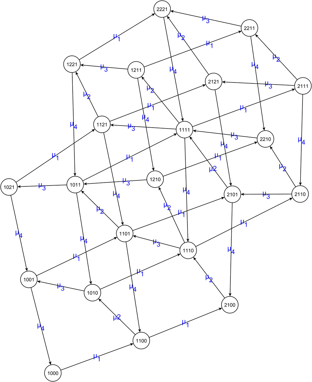
Figure 5. The state transition diagram of a production line with K = 4 stations. It has 21 vertices and 56 transitions, and the graph is the Algorithm’s outcome.

Figure 6

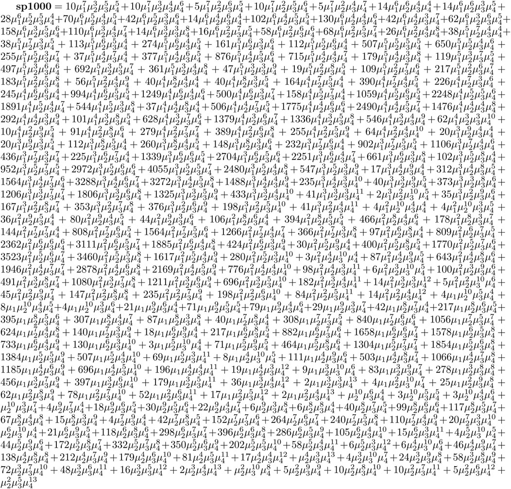
Figure 6. The spanning polynomial of the system state “1000” for a system of K = 4 stages without buffers.

The C++ code of the supplementary material was used to compare the MARKOV algorithm and the exact solution using the 194,481 line configurations used in Boulas et al. (2021) with μ_i∈[0.9,1.1], i = 1,2,3,4. These data were used to develop some Artificial Intelligence approaches, i.e., Genetic Programming and a hybrid scheme of Genetic Programming and Genetic Algorithms, to express the throughput by small size approximation formulas for K = 4 stations, among others. Table 2 shows the performance of the MARKOV algorithm, and our study shows that the highest difference in 194,481-line configurations is 5.37 × 10⁻⁷, which proves that the MARKOV algorithm gives accurate results. Any deviation is due to rounding to six digits. The CPU time for throughput estimation for all 194,481-line configurations was 1,141 s (19.02 min) for the exact formula, while by the MARKOV algorithm as specified in the prodline software (see (Papadopoulos et al., 2009) 692,302 s (8.01 days) using the same computer, an i7 CPU 970 running at 2.67 GHz, with eight cores and 16 GB RAM.

Table 2

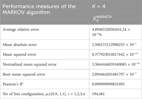
Table 2. The performance measures of the MARKOV algorithm were compared against the exact formula for K = 4 station production lines without intermediate buffers.

It should be noted that the exact throughput formula for lines with K = 4 stations contains 2,317,824 monomials in the numerator and 4,502,592 monomials in the denominator, whose exponents sum to 20. To ensure that the 21 spanning polynomials, i.e., each for each system state, are the exact solutions of the Equation $\mathit{\pi }·\mathit{Q}=\mathbf{0}$, the procedure described for lines with K = 3 stations was followed using Python’s SymPy module library, see Meurer et al. (2017). Thus, using the spanning polynomials coded in the supplementary material, one can access exact formulas and use them for any system performance measure that can be extracted from the underlying MARKOV chain.

4.4 Case K ≥ 5

For the case of a system of K = 5 stages, the Algorithm figures out the state transition diagram, a graph with 55 vertices (system states) and 145 edges (transition from one state to another). There are 34 edges for μ₁ and μ₅, 26 for μ₂ and μ₄, and 25 for μ₃. For this kind of graph, the monomials exponent sum is equal to 54, and their coefficients are relative to their number, which is a function of the anti-arborescences number or equivalently to the number of spanning trees when the direction edge is reversed.

A variation of the matrix-tree theorem is used to estimate the number of spanning trees in a directed graph. See (Boulas et al., 2024a) of our work for details. The number of spanning trees κ(Γ) in a directed graph Γ=(V, E) is equal to the determinant of the Laplacian matrix L of the graph Γ.

Table 3 presents the number of anti-arborescences for each of the 55 states of the line of K = 5 stages. The ‘10000’ state anti-arborescence number denotes the tremendous growth of the spanning monomial number. In our experiment, after 3 months of execution (when the execution stopped), the Algorithm, coded in C++, enumerated one million anti-arborescences of state ‘10000’ every 33 seconds. With that rate, finding all anti-arborescences of state ‘10000’ requires 1.109.000 years, while the whole graph estimation requires 140.000.000 years. Also, the computer integer number for the enumeration was exhausted many times through the execution; someone must use special C++ libraries to handle huge integers. That gives a sense of the size, which the exact formulas have even for short serial production lines.

Table 3

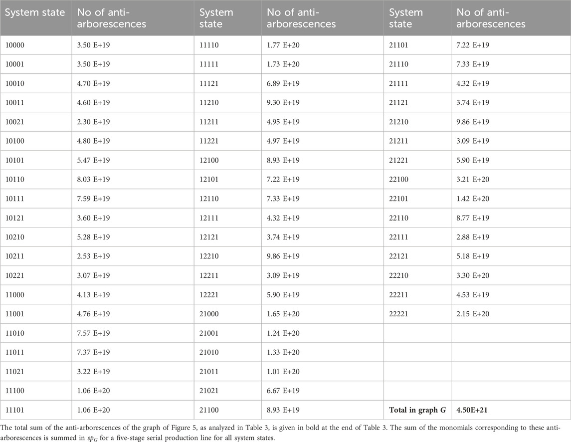
Table 3. The number of anti-arborescences for every state of K = 5 stages production line without intermediate buffers.

Following the same method for estimating spanning trees in a graph, Table 4 has been compiled. It shows the total number of the anti-arborescences for each stage, from one to eight.

Table 4

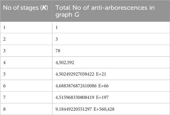
Table 4. The total number of anti-arborescences in the whole-state transition diagrams of K = 1 to 8-stage serial production lines without buffers.

4.5 Some insights into the bowl phenomenon can be obtained by the spanning tree’s structure

With the treatment of the Algorithm outcomes, Table 5 has been created. It presents the number of occurrences of every mean service rate for each machine in the corresponding graph, i.e., the state transition diagram. Let us assume that the corresponding exponent for every mean service rate μ_i, i∈{1.2, … , K} is x_i, i∈{1.2, … , K}, i.e., x₁ refers to μ₁, x₂ refers to μ₂ and so on. The number of occurrences of each mean service rate as an edge’s weight in the transition rate diagram, let it be o_i, i∈{1.2, … , K}, i.e., o₁ refers to μ₁, o₂ refers to μ₂ and so on. The integer values x_i can take are the components of vector x_i = [0.1, … , o_i]. The number of every possible combination that produces monomials is the Cartesian product x₁×x₂×… × x_K. If the number of system states is S, the maximum feasible set of monomials, M, is produced by Equation 19. The actual number of different monomials may be different. For K = 2 and K = 3, the feasible and actual number of monomials are the same, 3 and 24, respectively. For K = 4, the actual number is 1,018 monomials, while the cardinality of M is 1,163 monomials. For K = 5 and K = 6, the feasible number of monomials is 307,681 and 443889258, respectively, the upper limit of the different monomials that can appear in the sp_G.

${\mathit{x}}_1\times {\mathit{x}}_2\times ...\times {\mathit{x}}_K=\left[0,1,...,o_1\right]\times \left[0,1,...,o_2\right]\times ....\times \left[0,1,...,o_K\right]\text{\hspace{0.17em}constrained\hspace{0.17em}by\hspace{0.17em}}{\displaystyle \sum _{i=1}^K}{x}_i=S-1(19)$

Table 5

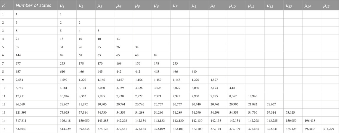
Table 5. The number of mean service rates as the weight of the transitions in state transition diagrams of K = 1 to 15 serial production lines without intermediate buffers.

Table 6 is the result of another observation obtained from the Algorithm outcomes if we record the number of occurrences of each mean service rate in all spanning trees of the graph for the number of stages K = 1 to 4. Examining the data sets in Tables 5, 6 by the number of stages in the production line shows a symmetric bowl pattern, with the mean service rates of middle stages underrepresented in the occurrences compared to the outlying ones. That means not all stages are equally involved in the spanning polynomial configuration and the exact formulas of systems’ performance metrics. This fact can explain the well-known bowl phenomenon; see about that in the book by Papadopoulos et al. (2009).

Table 6

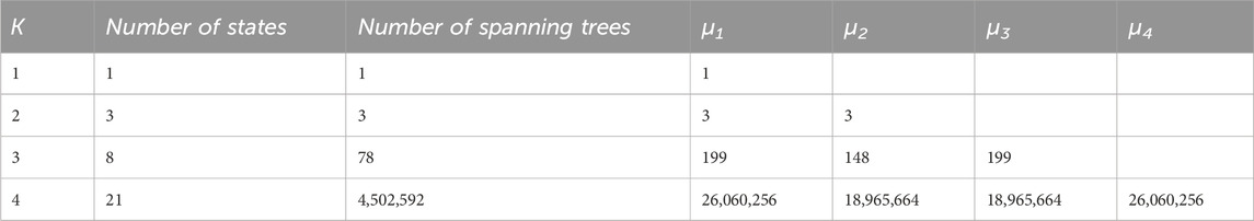
Table 6. The mean service rate occurrences in all spanning trees of transition state diagrams for K = 1 to 4 serial production lines without intermediate buffers.

4.6 The throughput estimation for the case of K stages balanced lines using a new genetic programming formula

This section introduces a new, straightforward formula for estimating throughput in balanced lines with K stages, utilizing genetic programming techniques. The formula takes advantage of the formulas structural insights gained from this work.

With the knowledge we have obtained of the formulas derived through the methodology of using spanning trees of state transition diagrams, we know that the MARKOV algorithm, if we use it for K stages and μ_i = 1 for i∊{1, 2, … , K}, will provide the maximum utilization of the serial production line. That is because we have the factorizations and simplifications in the numerator and denominator of the same powers equal to the number of system states minus 1. Despite the enormous size of the operations, since the mean service rate μ_i = 1 for i∊{1, 2, … , K} is used, the result of the operations is identical to the result of the MARKOV algorithm, which gives the throughput, however, because μ_i = 1 for i∊{1, 2, … , K}, it is identical to the maximum utilization ρ_max, see Equation 21.

As shown in Section 4.3, the results of the MARKOV algorithm are identical to the exact solutions of the system for four stages, with only the rounding errors from the arithmetic operations. Previous work (Heavey et al., 1993) has shown that the results of the MARKOV algorithm provide the exact solutions under the restriction of the rounding error. For this reason, the exact MARKOV algorithm is used to construct a data set for training a genetic programming system (Koza, 1992) implemented in HeuristicLab software (Wagner et al., 2014). Moreover, algebraic manipulations to generate a tractable formula that approximates the throughput X_K for perfectly balanced K-stage lines K = 1, 2, … ,13 and μ_i = μ, i = 1.2, … , K. We use the values for K = 1 to 12 stages as the training set. For the 13th stage, we verify the value published in (Fernandes et al. (2013b). The result shows that the formula derived from GP presented in Equation 20 is accurate up to the sixth decimal digit. Numerous tests performed showed convergence to the sixth decimal place in throughput using the MARKOV algorithm for different values of K = 1, 2, … ,13 and μ_i = μ, i = 1.2, … , K, which is the case for perfectly balanced lines.

The Genetic Programming formula for maximum utilization for perfectly balanced K-stage lines K = 1, 2, … ,13 is shown by Equation 20 and the corresponding throughput for the production line by Equation 21 where K = 1, 2, … ,13 and μ_i = μ, i = 1.2, … , K.

${\rho }_{\max }=0.3724972+\frac{0.0186781}{1.6617246K+19.4375419}+\frac{0.0293145e^{2.0225831e^{-0.6311543K}}+0.5288344+\frac{0.0118095}{K}}{K}(20)$

${\mathrm{X}}_{\mathrm{K}}=\mathrm{\mu }{\mathrm{\rho }}_{\max }(21)$

5 Discussion

This paper presents an implementation of the algorithmic approach given in (Boulas et al., 2025) of our work, which corresponds to a general procedure for extracting stationary probabilities of an arbitrary irreducible Markov chain and uses the proposed Algorithm to solve problems of performance measures of short serial production lines without buffers. A new algorithm is introduced to construct the state transition diagrams for that system. We use the two algorithmic approaches to extend Hunt’s work (Hunt, 1956) for all system performance measures for a short line of three stages without buffers. The Algorithm solves a system with K = 4 stages without buffers and gives its stationary probabilities. This is the first time an accurate formula has appeared in the literature for production lines with four stations without intermediate buffers. The Algorithm can provide accurate analytic formulas for all performance measures of small-size production systems, throughput, maximum utilization, and all performance measures obtained from the underlying Markov chain. The system behavior is elaborated on the graph representing the state transition diagram. The proposed Algorithm directly creates the system states and the system’s state transition diagram under the model assumption, providing the details of the transitions between the system states. The latter is very informative about understanding the complexity and operation of that kind of system. The overall methodology solves a production line without intermediate buffers for any number of stations by simply enumerating the anti-arborescences of the graph. That is a tedious task in practice due to the enormous number of anti-arborescences.

The exact formulas generated by the Algorithm are so extensive that they modify the concept of closed-form formulas. For example, for the system with K = 4 stations, until the coding in C++ of the code in the supplementary material, the value of the formulas was estimated with the help of a parser that passes through a matrix of coefficients and exponents of the polynomials. In our experience (Boulas et al., 2021), this parser operation was very similar to the evaluation of genetic programming trees; the genetic programming tree is a spanning tree. The difference in genetic programming is that its solution is only one spanning tree of many, while the exact solution consists of many spanning trees of the same size. The enormous number of anti-arborescences in graphs for lines with K ≥ 5 stations leads to solutions that require memory, computational power, special libraries, and reliable computing systems. It is an impressive and expected realization that the formula no longer gives exact results (the equilibrium equations cannot be solved analytically) when even a single digit changes from the existing millions of spanning polynomials.

Because of the use of graphs and the concept of spanning trees, the overall methodology is based on the top of the automata theory. The computation tree in Figure 4, one of the eight that express the system behavior, functions as an operation instruction manual of the system. It is noted that the number of these computation trees increases following the number of the system state, see Table 5 and their depth increases to the number of the state minus 1. Also, the number of the branches T_i (T_i, i = 1, 2, … , 8 in Figure 4) increases tremendously according to Table 3 to give a sense of it. The exact solutions consider all these transitions instead of the approximate ones, which somehow group them and relate them mathematically.

Conversely, simulation samples and builds a subset of these transitions to obtain results for a reduced system. As sampling improves, the results’ accuracy improves, and the simulation’s quality improves. However, all this complexity and the size of the possible transitions of the systems show that even with the more detailed available method for elaborating that kind of system, the simulation works statistically on a small part of the system’s transition. That observation is critical and valuable when we want to develop formulas of acceptable accuracy, but small size based on a small but representative number of appropriately chosen spanning trees.

The enormous size of exact formulas can be a problem. In this work, we have treated the most straightforward production line. More complicated lines, i.e., buffers, phase-type distributions, and unreliable machines, can lead to more extensive and more complicated formulas with a ratio of two polynomials. These formulas may serve as structural components of methods like decomposition (Gershwin, 1987). Moreover, graph theory may help explain the most profound function of decomposition methods. However, the enormous size of the exact formulas is also an opportunity because obtaining exact formulas for longer production lines is a computational challenge for computers that may have yet to be invented. Combining numerical answers about stationary probabilities of production lines using algorithms such as MARKOV and the analytic solution could be attractive for creating benchmarking problems or algorithms that can test computational systems such as quantum computers (Steane, 1998), comparing the time to find the anti-arborescences and the accuracy of the results.

Artificial intelligence methods, such as genetic programming, remain attractive. Previous work has shown that genetic programming offers a remarkable ability to recognize the deeper structure of the solution, whether we know it or not. Artificial intelligence and machine learning methods with appropriate specifications for the output’s accuracy, scope, or usability in estimating the performance of production lines may play an essential role in this field for the following years.

6 Conclusions and further research

In this work, an Algorithm has been developed to express the state transition diagram for the short serial production line to obtain the stationary probabilities for K = 2,3,4 stages in symbolic form using the method introduced in Part I in this work (Boulas et al., 2024a). The solutions provided are exact as they verify the equilibrium equations of the systems. To our knowledge, exact analytic solutions for production lines with K = 3 and 4 stations and no intermediate buffers are given for the first time in literature, and the solution size for more extensive lines is also estimated. The constant sum of their exponents characterizes the monomials due to the fixed number of anti-arborescence edges, which equals the number of system states minus one, transforming the exact solutions for K ≥ 5 stations to a vast size. The solution is a closed-form formula of two polynomials ratio.

When enumerating the transitions in the state transition diagram, some observations were made regarding the well-known bowl phenomenon in production systems. These have to do with the variation in the number of transitions, their symmetry, and their reversibility. Finally, using genetic programming as an artificial intelligence method, a simple formula specifies the throughput for a fully balanced K-stage line where the mean service rates of each stage are identical.

Future research might investigate other types of production lines. In terms of applications, our team is working on production lines, supply chains, and queueing networks to obtain mathematical formulas expressing the performance metrics of these systems. Production lines with buffers and other topologies are of interest. Also, the quantification between the spanning trees and bowl phenomenon is promising. Exploring the possibilities of parallel running Gabow and Myers’ Algorithm is essential to finding the spanning trees rooted from the same node. Finally, recursive methods such as decomposition can be extended to other performance measures using the exact formulas for their estimation as structural elements (building blocks). Currently, the focus of our research regarding the presented methodology is related to systems of phase type distributions as well as to similar problems existing in logistics systems and in systems containing unreliable lines.

It should also be noted that the tremendous evolution of computer technology provided tools that made calculations more efficient and effective for finding solutions to previously unsolved problems. In addition, through evolutionary computing and genetic programming, modern computer science made it possible to obtain approximate formulas of high accuracy for short serial production lines. Accuracy can be further improved for more extensive lines if more careful sampling of training data is used, embodying information regarding the unique characteristics of formulas or other predictive models. The present work shows the immense size of the exact closed-form formulas expressing the stationary probabilities and performance measures. This size makes the AI-oriented methods attractive for forming approximate solutions for performance measurement in problems of interest. A comparison of the formulas for lines with K = 4 or K = 5 stations presented in Boulas et al. (2021) with the exact formulas for thousands or millions of monomials presented or mentioned in the present work makes this claim credible. Conversely, production lines can provide helpful benchmark paradigms for artificial intelligence. There is a commonplace in research on assembly line work, computational complexity, and artificial intelligence that will benefit all disciplines involved.

Data availability statement

The original contributions presented in the study are included in the article/supplementary material, further inquiries can be directed to the corresponding author.

Author contributions

KB: Conceptualization, Investigation, Methodology, Software, Visualization, Writing – original draft, Writing – review and editing. GD: Conceptualization, Project administration, Supervision, Validation, Writing – original draft, Writing – review and editing. CP: Investigation, Project administration, Supervision, Validation, Writing – original draft, Writing – review and editing.

Funding

The author(s) declare that no financial support was received for the research and/or publication of this article.

Conflict of interest

The authors declare that the research was conducted in the absence of any commercial or financial relationships that could be construed as a potential conflict of interest.

Publisher’s note

All claims expressed in this article are solely those of the authors and do not necessarily represent those of their affiliated organizations, or those of the publisher, the editors and the reviewers. Any product that may be evaluated in this article, or claim that may be made by its manufacturer, is not guaranteed or endorsed by the publisher.

Supplementary material

The Supplementary Material for this article can be found online at: https://www.frontiersin.org/articles/10.3389/fmtec.2025.1439429/full#supplementary-material

References

Aboutaleb, A., Kang, P. S., Hamzaoui, R., and Duffy, A. (2017). Standalone closed-form formula for the throughput rate of asynchronous normally distributed serial flow lines. J. Manuf. Syst. 43, 117–128. doi:10.1016/j.jmsy.2016.12.006

CrossRef Full Text | Google Scholar

Alkhalefah, H., Umer, U., Abidi, M. H., and Elkaseer, A. (2023). Development and numerical optimization of a system of integrated agents for serial production lines. Processes 11, 1578. doi:10.3390/pr11051578

CrossRef Full Text | Google Scholar

Altiok, T. (1997). Performance analysis of manufacturing systems. New York, NY: Springer New York. doi:10.1007/978-1-4612-1924-8

CrossRef Full Text | Google Scholar

Arinez, J. F., Chang, Q., Gao, R. X., Xu, C., and Zhang, J. (2020). Artificial intelligence in advanced manufacturing: current status and future outlook. J. Manuf. Sci. Eng. 142. doi:10.1115/1.4047855

CrossRef Full Text | Google Scholar

Ayvaz, S., and Alpay, K. (2021). Predictive maintenance system for production lines in manufacturing: a machine learning approach using IoT data in real-time. Expert Syst. Appl. 173, 114598. doi:10.1016/j.eswa.2021.114598

CrossRef Full Text | Google Scholar

Bai, Y., Tu, J., Yang, M., Zhang, L., and Denno, P. (2021). A new aggregation algorithm for performance metric calculation in serial production lines with exponential machines: design, accuracy and robustness. Int. J. Prod. Res. 59, 4072–4089. doi:10.1080/00207543.2020.1757777

CrossRef Full Text | Google Scholar

Baker, K. R., Powell, S. G., and Pyke, D. F. (1994). A predictive model for the throughput of unbalanced, unbuffered three-station serial lines. IIE Trans. 26, 62–71. doi:10.1080/07408179408966619

CrossRef Full Text | Google Scholar

Basu, R. N. (1977). The interstage buffer storage capacity of non-powered assembly lines A simple mathematical approach. Int. J. Prod. Res. 15, 365–382. doi:10.1080/00207547708943136

CrossRef Full Text | Google Scholar

Blumenfeld, D. E. (1990). A simple formula for estimating throughput of serial production lines with variable processing times and limited buffer capacity. Int. J. Prod. Res. 28, 1163–1182. doi:10.1080/00207549008942783

CrossRef Full Text | Google Scholar

Blumenfeld, D. E., and Li, J. (2005). An analytical formula for throughput of a production line with identical stations and random failures. Math. Problems Eng. 2005, 293–308. doi:10.1155/mpe.2005.293

CrossRef Full Text | Google Scholar

Boulas, K., Dounias, G., and Papadopoulos, C. (2017). “Approximating throughput of small production lines using genetic programming,” in Operational research in business and economics: 4th international symposium and 26th national conference on operational research, chania, Greece, june 2015. Editors E. Grigoroudis, and M. Doumpos (Cham: Springer International Publishing), 185–204. doi:10.1007/978-3-319-33003-7_9

CrossRef Full Text | Google Scholar

Boulas, K., Dounias, G., Papadopoulos, C., and Tsakonas, A. (2015). “Acquisition of accurate or approximate throughput formulas for serial production lines through genetic programming,” in Proceedings of the 4th international symposium and 26th national conference on operational research (Chania, Greece: Hellenic Operational Research Society), 128–133. Available online at: http://mde-lab.aegean.gr/research-material.

Google Scholar

Boulas, K., Tzanetos, A., and Dounias, G. (2018). Acquisition of approximate throughput formulas for serial production lines with parallel machines using intelligent techniques., in Proceedings of the 10th Hellenic Conference on Artificial Intelligence, 18. Greece: Rio Patras, 1–18:7. doi:10.1145/3200947.3201028

CrossRef Full Text | Google Scholar

Boulas, K. S., Dounias, G. D., and Papadopoulos, C. T. (2021). A hybrid evolutionary algorithm approach for estimating the throughput of short reliable approximately balanced production lines. J. Intelligent Manuf. 34, 823–852. doi:10.1007/s10845-021-01828-6

CrossRef Full Text | Google Scholar

Boulas, K. S., Dounias, G. D., and Papadopoulos, C. T. (2025). “Extraction of exact symbolic stationary probability formulas for Markov chains in finite space with application to production lines. Part I: description of methodology,” in Frontiers in manufacturing technology. Submitted in.

Google Scholar

Buzacott, J. A., and Shanthikumar, J. G. (1992). Design of manufacturing systems using queueing models. Queueing Syst. 12, 135–213. doi:10.1007/BF01158638

CrossRef Full Text | Google Scholar

Buzacott, J. A., and Shanthikumar, J. G. (1993). Stochastic models of manufacturing systems. New Jersey: Prentice Hall.

Google Scholar

Can, B., and Heavey, C. (2009). “Sequential metamodelling with genetic programming and particle swarms,” in Proceedings of the 2009 (Winter Simulation Conference (WSC) (Austin, TX, USA: IEEE), 3150–3157. doi:10.1109/WSC.2009.5429276

CrossRef Full Text | Google Scholar

Can, B., and Heavey, C. (2011). Comparison of experimental designs for simulation-based symbolic regression of manufacturing systems. Comput. and Industrial Eng. 61, 447–462. doi:10.1016/j.cie.2011.03.012

CrossRef Full Text | Google Scholar

Can, B., and Heavey, C. (2012). A comparison of genetic programming and artificial neural networks in metamodeling of discrete-event simulation models. Comput. and Operations Res. 39, 424–436. doi:10.1016/j.cor.2011.05.004

CrossRef Full Text | Google Scholar

Cañas, H., Mula, J., Díaz-Madroñero, M., and Campuzano-Bolarín, F. (2021). Implementing Industry 4.0 principles. Comput. and Industrial Eng. 158, 107379. doi:10.1016/j.cie.2021.107379

CrossRef Full Text | Google Scholar

Cui, P.-H., Wang, J.-Q., Li, Y., and Yan, F.-Y. (2021). Energy-efficient control in serial production lines: modeling, analysis and improvement⋆. J. Manuf. Syst. 60, 11–21. doi:10.1016/j.jmsy.2021.04.002

CrossRef Full Text | Google Scholar

Dallery, Y., and Gershwin, S. B. (1992). Manufacturing flow line systems: a review of models and analytical results. Queueing Syst. 12, 3–94. doi:10.1007/BF01158636

CrossRef Full Text | Google Scholar

Dar-El, E. M., and Mazer, A. (1989). Predicting the performance of unpaced assembly lines where one station variability may be smaller than the others. Int. J. Prod. Res. 27, 2105–2116. doi:10.1080/00207548908942678

CrossRef Full Text | Google Scholar

Dhouib, K., Gharbi, A., and Mejri, M. (2010). “Throughput variability of homogeneous transfer lines subject to operation-dependant failures,” in 8th international conference on modeling and simulation (MOSIM’10), USA, 2010-05-10, 1290–1299. Hammamet, Tunisia: Lavoisier).

Google Scholar

Fernandes, P., O’Kelly, M. E., Papadopoulos, C. T., and Sales, A. (2013a). Analysis of exponential unreliable production lines using Kronecker descriptors. Germany: Kloster Seeon, 1–9.

Google Scholar

Fernandes, P., O’Kelly, M. E. J., Papadopoulos, C. T., and Sales, A. (2013b). Analysis of exponential reliable production lines using Kronecker descriptors. Int. J. Prod. Res. 51, 4240–4257. doi:10.1080/00207543.2012.754550

CrossRef Full Text | Google Scholar

Fragapane, G., Ivanov, D., Peron, M., Sgarbossa, F., and Strandhagen, J. O. (2022). Increasing flexibility and productivity in Industry 4.0 production networks with autonomous mobile robots and smart intralogistics. Ann. Operations Res. 308, 125–143. doi:10.1007/s10479-020-03526-7

CrossRef Full Text | Google Scholar

Gabow, H. N., and Myers, E. W. (1978). Finding all spanning trees of directed and undirected graphs. SIAM J. Comput. 7, 280–287. doi:10.1137/0207024

CrossRef Full Text | Google Scholar

Gershwin, S. B. (1987). An efficient decomposition method for the approximate evaluation of tandem queues with finite storage space and blocking. Operations Res. 35, 291–305. doi:10.1287/opre.35.2.291

CrossRef Full Text | Google Scholar

Gershwin, S. B. (1994). Manufacturing systems engineering. Englewood Cliffs, N.J: PTR Prentice Hall.

Google Scholar

Gershwin, S. B. (2018). The future of manufacturing systems engineering. Int. J. Prod. Res. 56, 224–237. doi:10.1080/00207543.2017.1395491

CrossRef Full Text | Google Scholar

L. Ghezzi, D. Hömberg, and C. Landry (2017). Math for the digital factory (Cham: Springer International Publishing). doi:10.1007/978-3-319-63957-4

CrossRef Full Text | Google Scholar

Hatcher, J. M. (1969). The effect of internal storage on the production rate of a series of stages having exponential service times. AIIE Trans. 1, 150–156. doi:10.1080/05695556908974427

CrossRef Full Text | Google Scholar

Haydon, B. J. (1973). The behaviour of systems of finite queues. Kensington, New South Wales. Australia: The University of New South Wales.

Google Scholar

Heavey, C., Papadopoulos, H. T., and Browne, J. (1993). The throughput rate of multistation unreliable production lines. Eur. J. Operational Res. 68, 69–89. doi:10.1016/0377-2217(93)90077-Z

CrossRef Full Text | Google Scholar

Hillier, F. S., and Boling, R. W. (1966). The effects of some design factors on the efficiency of production lines with variable operation times. J. Industrial Eng. 17, 651–658.

Google Scholar

Hillier, F. S., and Boling, R. W. (1967). Finite queues in series with exponential or Erlang service times—a numerical approach. Operations Res. 15, 286–303. doi:10.1287/opre.15.2.286

CrossRef Full Text | Google Scholar

Hira, D. S., and Pandey, P. C. (1987). Efficiency of manual flow line systems—predictive equations. Int. J. Prod. Res. 25, 603–614. doi:10.1080/00207548708919864

CrossRef Full Text | Google Scholar

Holland, J. H. (1992). “Adaptation in natural and artificial systems: an introductory analysis with applications to biology, control,” in And artificial intelligence. Cambridge, Mass: 1st MIT Press. doi:10.7551/mitpress/1090.001.0001

CrossRef Full Text | Google Scholar

Hunt, G. C. (1956). Sequential arrays of waiting lines. Operations Res. 4, 674–683. doi:10.1287/opre.4.6.674

CrossRef Full Text | Google Scholar

Kang, P. S., and Bhatti, R. S. (2019). Continuous process improvement implementation framework using multi-objective genetic algorithms and discrete event simulation. Bus. Process Manag. J. 25, 1020–1039. doi:10.1108/BPMJ-07-2017-0188

CrossRef Full Text | Google Scholar

Koza, J. R. (1992). Genetic programming: on the programming of computers by means of natural selection. Cambridge, MA: MIT Press.

Google Scholar

Li, L., Qian, Y., Du, K., and Yang, Y. (2016). Analysis of approximately balanced production lines. Int. J. Prod. Res. 54, 647–664. doi:10.1080/00207543.2015.1015750

CrossRef Full Text | Google Scholar

Magazine, M. J., and Stecke, K. E. (1996). Throughput for production lines with serial work stations and parallel service facilities. Perform. Eval. 25, 211–232. doi:10.1016/0166-5316(95)00005-4

CrossRef Full Text | Google Scholar

Magnanini, M. C., and Tolio, T. (2023). A Markovian model of asynchronous multi-stage manufacturing lines fabricating discrete parts. J. Manuf. Syst. 68, 325–337. doi:10.1016/j.jmsy.2023.04.006

CrossRef Full Text | Google Scholar

Martin, G. E. (1993). Predictive formulae for unpaced line efficiency. Int. J. Prod. Res. 31, 1981–1990. doi:10.1080/00207549308956835

CrossRef Full Text | Google Scholar

Meurer, A., Smith, C. P., Paprocki, M., Čertík, O., Kirpichev, S. B., Rocklin, M., et al. (2017). SymPy: symbolic computing in Python. PeerJ Comput. Sci. 3, e103. doi:10.7717/peerj-cs.103

CrossRef Full Text | Google Scholar

Mishra, A., Acharya, D., Rao, N. P., and Sastry, G. P. (1985). Composite stage effects in unbalancing of series production systems. Int. J. Prod. Res. 23, 1–20. doi:10.1080/00207548508904687

CrossRef Full Text | Google Scholar

Muth, E. J. (1977). “Numerical methods applicable to a production line with stochastic servers,” in Algorithmic methods in probability. Editor M. F. Neuts (North-Holland Amsterdam), 143–159.

Google Scholar

Muth, E. J. (1984). Stochastic processes and their network representations associated with a production line queuing model. Eur. J. Operational Res. 15, 63–83. doi:10.1016/0377-2217(84)90049-3

CrossRef Full Text | Google Scholar

Muth, E. J. (1987). “An update on analytical models of serial transfer lines,” in Gainesville FL USA: Department of Industrial and Systems Engineering, University of Florida. University of Florida Gainesville FL.

Google Scholar

Muth, E. J., and Alkaff, A. (1987). The throughput rate of three-station production lines: a unifying solution. Int. J. Prod. Res. 25, 1405–1413. doi:10.1080/00207548708919922

CrossRef Full Text | Google Scholar

Panwalkar, S. S., and Smith, M. L. (1979). A predictive equation for average output of K stage series systems with finite interstage queues. AIIE Trans. 11, 136–139. doi:10.1080/05695557908974453

CrossRef Full Text | Google Scholar

Papadopoulos, C., Tsakonas, A., and Dounias, G. (2002). “Combined use of genetic programming and decomposition techniques for the induction of generalized approximate throughput formulas in short exponential production lines with buffers,”. Proceedings of the 30th international conference on computers and industrial engineering. Editors C. Papadopoulos, and E. Triantaphyllou (Greece: Tinos Island), 6.

Google Scholar

Papadopoulos, C. T., Li, J., and O’Kelly, M. E. J. (2019). A classification and review of timed Markov models of manufacturing systems. Comput. and Industrial Eng. 128, 219–244. doi:10.1016/j.cie.2018.12.019

CrossRef Full Text | Google Scholar

Papadopoulos, C. T., Vidalis, M. J., O’Kelly, M. E. J., and Spinellis, D. (2009). Analysis and design of discrete Part Production lines. New York, NY: Springer New York. doi:10.1007/978-0-387-89494-2_1

CrossRef Full Text | Google Scholar

Papadopoulos, H. T. (1996). An analytic formula for the mean throughput of K-station production lines with no intermediate buffers. Eur. J. Operational Res. 91, 481–494. doi:10.1016/0377-2217(95)00113-1

CrossRef Full Text | Google Scholar

Papadopoulos, H. T., Heavey, C., and O’Kelly, M. E. J. (1989). Throughput rate of multistation reliable production lines with inter station buffers: (I) Exponential Case. Comput. Industry 13, 229–244. doi:10.1016/0166-3615(89)90113-9

CrossRef Full Text | Google Scholar

Papadopoulos, H. T., Heavey, C., and O’Kelly, M. E. J. (1990). Throughput rate of multistation reliable production lines with inter station buffers (II) Erlang case. Comput. Industry 13, 317–335. doi:10.1016/0166-3615(90)90004-9

CrossRef Full Text | Google Scholar

Papadopoulos, H. T., and O’Kelly, M. E. J. (1993). Exact analysis of production lines with no intermediate buffers. Eur. J. Operational Res. 65, 118–137. doi:10.1016/0377-2217(93)90147-F

CrossRef Full Text | Google Scholar

Rao, N. P. (1975a). On the mean production rate of a two-stage production system of the tandem type. Int. J. Prod. Res. 13, 207–217. doi:10.1080/00207547508942987

CrossRef Full Text | Google Scholar

Rao, N. P. (1975b). Two-stage production systems with intermediate storage. AIIE Trans. 7, 414–421. doi:10.1080/05695557508975025

CrossRef Full Text | Google Scholar

Rao, N. P. (1976a). A generalization of the ‘bowl phenomenon’ in series production systems. Int. J. Prod. Res. 14, 437–443. doi:10.1080/00207547608956617

CrossRef Full Text | Google Scholar

Rao, N. P. (1976b). A viable alternative to the ‘method of stages’ solution of series production systems with Erlang service times. Int. J. Prod. Res. 14, 699–702. doi:10.1080/00207547608956388

CrossRef Full Text | Google Scholar

Sankhye, S., and Hu, G. (2020). Machine learning methods for quality prediction in production. Logistics 4, 35. doi:10.3390/logistics4040035

CrossRef Full Text | Google Scholar

Scale, I. E. (1972). The analysis and design of multiple-parallel production lines with interaction and feedback. Australia: University of Newcastle.

Google Scholar

Subramaniyan, M., Skoogh, A., Bokrantz, J., Sheikh, M. A., Thürer, M., and Chang, Q. (2021). Artificial intelligence for throughput bottleneck analysis – state-of-the-art and future directions. J. Manuf. Syst. 60, 734–751. doi:10.1016/j.jmsy.2021.07.021

CrossRef Full Text | Google Scholar

Wagner, S., Kronberger, G., Beham, A., Kommenda, M., Scheibenpflug, A., Pitzer, E., et al. (2014). “Architecture and design of the HeuristicLab optimization environment,” in Advanced methods and applications in computational intelligence. Editors R. Klempous, J. Nikodem, W. Jacak, and Z. Chaczko (Heidelberg: Springer International Publishing), 197–261. Available online at: http://link.springer.com/chapter/10.1007/978-3-319-01436-4_10.

CrossRef Full Text | Google Scholar