Turing instability mechanism of short-memory formation in multilayer FitzHugh-Nagumo network

Introduction: The study of brain function has been favored by scientists, but the mechanism of short-term memory formation has yet to be precise.

Research problem: Since the formation of short-term memories depends on neuronal activity, we try to explain the mechanism from the neuron level in this paper.

Research contents and methods: Due to the modular structures of the brain, we analyze the pattern properties of the FitzHugh-Nagumo model (FHN) on a multilayer network (coupled by a random network). The conditions of short-term memory formation in the multilayer FHN model are obtained. Then the time delay is introduced to more closely match patterns of brain activity. The properties of periodic solutions are obtained by the central manifold theorem.

Conclusion: When the diffusion coeffcient, noise intensity np, and network connection probability p reach a specific range, the brain forms a relatively vague memory. It is found that network and time delay can induce complex cluster dynamics. And the synchrony increases with the increase of p. That is, short-term memory becomes clearer.

1. Introduction

In 1952, Alan Hodgkin and Andrew Huxley developed the famous Hodgkin-Huxley (HH) model based on nerve stimulation potential data of squid. Due to the high dimension and computational complexity of the HH model, Richard FitzHugh and J.Nagumo simplified the HH model and established the FHN model. In the actual nerve conduction process, there is a certain time delay in signal transmission, which caused a lot of research on the FHN model with time delay. Wang et al. studied bifurcation and synchronization (1), bifurcation structure (2), Fold-Hopf bifurcation (3), periodic oscillation (4), and global Hopf bifurcation (5) of coupled FHN model with time delay. Yu et al. (6) found that the noise level can change the signal transmission performance in the FHN network, and the delay can cause multiple stochastic resonances. Gan et al. (7) also found that appropriate delay can induce stochastic resonances in FHN scale-free networks and devoted themselves to extending the range of stochastic resonance on complex neural networks. Zeng et al. (8) found that, unlike noise, the system undergoes a phase transition as the time delay increases. Bashkirtseva and Ryashko analyzed the excitability of the FHN model using the stochastic sensitivity function technique and proposed a new method for analyzing attractors (9). In addition, it is found that there are very complex dynamic phenomena in the FHN model. Rajagopal et al. (10) studied chaos and periodic bifurcation diagrams under different excitation currents and found that the dynamic behavior of the nodes alters dramatically after the introduction of Gaussian noise. Iqbal et al. (11) studied robust adaptive synchronization of a ring-coupled uncertain chaotic FHN model and proposed a scheme to synchronize the coupled neurons under external electrical stimulation. Feng et al. studied the influence of external electromagnetic radiation on the FHN model. And they found that periodic, quasi-periodic, and chaotic motions would occur in different frequency intervals when the external electromagnetic radiation was in the form of a cosine function (12).

In the same year, the HH model was proposed, Turing discovered that a stable uniform state would become unstable under certain conditions in a reaction-diffusion system, which attracted a lot of attention and was introduced into various fields. Liu et al. found that cross-diffusion could lead to Turing instability of periodic solutions (13, 14). Lin et al. analyzed the conditions of Turing-Hopf bifurcation and the spatiotemporal dynamics near the bifurcation point in diffusion neural networks with time delay (15). Mondal et al. studied the dynamical behaviors near the Turing-Hopf bifurcation points of the neural model. And they found that collective behaviors may be related to the generation of some brain pathologies (16). Qu and Zhang studied the conditions required for various bifurcations in the FHN diffusion system under Neumann boundary conditions and extended them to coupled FHN model (17). With the boom of complex networks in recent years, many scholars have begun to study the Turing pattern under the network (18–22). Ren et al. extended these studies to multilayer networks (23, 24). Moreover, Tian et al. investigated pattern and Hopf bifurcation caused by time delay in the Small-World network, Barabasi-Albert free-scale network, and Watts-Strogatz network (25, 26). These studies take the pattern problem to a new level.

Researchers are keen to study some characteristic behaviors of the brain from the perspective of the network because the brain is a complex network system with hierarchical and modular structures (27). Neurons generate complex cluster dynamic behaviors through synaptic coupling to form brain function. Neurons with similar connection patterns usually have the same functional attributes (28). Experiments have shown that neurons far apart can fire simultaneously when the brain is stimulated and that this phenomenon persists when neurons are in the resting state. One of the brain's basic functions is remembering information, which can be a sensory stimulus or a text (29). The principle of memory formation is very complex and is still being explored. A classic view is that the realization of short-term memory in the brain depends on fixed point attractors (30, 31). Memory storage is maintained by the continuous activity of neurons, which persists even after the memory stimulus has been removed (32, 33). Goldman showed the fundamental mechanisms that generate sustained neuronal activity in feedforward and recurrent networks (33). Neurons release neurotransmitters that direct human activity when the brain receives the information. However, due to the noise and the existence of inhibitory neurons, information processing cannot always be synchronized in time, which leads to a certain delay in the recovery time of action potentials (34). And Yu et al. found that the delay will affect the transmission performance of sub-threshold signal and induce various chaotic resonances in coupled neural networks (35).

The state of neurons can be represented by patterns. The pattern no longer looks so smooth when the brain stores short-term memory. There is synchrony in the activity of neurons. In pattern dynamics, synchronization can be induced by Turing instability. Scholars have built various mathematical models and analyzed neurons using Turing dynamic theory to understand the mechanism of memory formation. Zheng et al. studied the effect of noise on the bistable state of the FHN model and explained the biological mechanism of short-term memory by the pattern dynamics theory (36). They also studied the conditions of Turing pattern generation in the Hindmarsh-Rose (HR) model and found that collected current and outgoing current greatly influenced neuronal activity and used this to explain the mechanism of short-term memory generation (37). Wang and Shi proposed the time-delay memristive HR neuron model, found multiple modes and coherence resonance, and speculated that it might be related to the memory effect of neurons (38). We study the FHN model under a multilayer network to get closer to the actual brain structure. The biological mechanism of short-term memory generation is explained by the pattern characteristics of the model. The article is structured as follows. In the next section, firstly, the stability of the equilibrium point in the FHN model is analyzed. Then the sufficient conditions for the Turing instability of the FHN model on the Cartesian product network are found using the comparison principle. Finally, the properties of periodic solutions in FHN multilayer networks are studied using the center manifold theorem. Explaining the mechanism of short-term memory by numerical simulation in Section 3.

2. Description of the FHN model

We consider the general FHN model

$\begin{array}{l}\frac{du}{dt}=c(u-u^3/3-av+I),\\ \frac{dv}{dt}=c(bu-v+d),& (1)\end{array}$

Where u is membrane potential, which is a fast variable, and v is recovery variable, which is a slow variable. I is the external input current. a, b represent respectively the intensity of action from v to u and from u to v. And the parameters c ≠ 0, d are constants. The equilibrium point of the system (Equation 1) satisfies u³ + 3(ab − 1)u + 3(ad − I) = 0. Therefore, we have the following conclusion.

Lemma 1 Let $\varpi =\frac{-1+\iota \sqrt{3}}{2}$ and $\varrho =\frac{3}{2}(ad-I)$, in which ι is the imaginary unit. The influence of parameters on the number of equilibrium of the system (Equation 1) is as follows.

(i) When ab − 1 = ad − I = 0, the equation has triple zero roots and the trace of the system (1) at that point is constant 0.

(ii) When Δ = ϱ² + (ab − 1)³ > 0, the equation has only one real root $\sqrt[3]{-\varrho +\sqrt{\Delta }}+\sqrt[3]{-\varrho -\sqrt{\Delta }}$.

(iii) When Δ = 0, ab ≠ 1 and ad ≠ I, the equation has two real roots $-2\sqrt[3]{\varrho }$ and $\sqrt[3]{\varrho }$, and the determinant at the second root $\sqrt[3]{\varrho }$ of system (1) is always 0.

(iv) When Δ < 0, the equation has three unequal real roots $\sqrt[3]{-\varrho +\sqrt{\Delta }}+\sqrt[3]{-\varrho -\sqrt{\Delta }}$, $\varpi \sqrt[3]{-\varrho +\sqrt{\Delta }}+{\varpi }^2\sqrt[3]{-\varrho -\sqrt{\Delta }}$, ${\varpi }^2\sqrt[3]{-\varrho +\sqrt{\Delta }}+\varpi \sqrt[3]{-\varrho -\sqrt{\Delta }}$.

Let U^* = (u^*, v^*) be the equilibrium point of the system (1). By coordinate transformation ū = u(t)−u^*, $\bar{v}=v(t)-v^{*}$, we get the following equivalent system. For convenience, u(t), v(t) are still used to denote ū, $\bar{v}$,

$\begin{array}{l}\frac{du}{dt}=a_{11}u+a_{12}v+f(u),\\ \frac{dv}{dt}=a_{21}u+a_{22}v,& (2)\end{array}$

where $a_{11}=c(1-u^{{*}^2})$, a₁₂ = −ac, a₂₁ = bc, a₂₂ = −c, $f(u)=-u^{*}{u}^2-\frac{u^3}{3}$. The corresponding determinant ${\Delta }_0=c^2(u^{{*}^2}+ab-1)$ and the trace $T{r}_0=-c{u}^{{*}^2}$. By the Routh-Hurwitz criterion, the equilibrium (0, 0) of the system (Equation 2) is stable if and only if (H 1) holds,

$\begin{array}{ll}c{u}^{{*}^2}>0\text{ and }{u}^{{*}^2}+ab-1>0.& (\mathrm{H\; 1})\end{array}$

2.1. FHN model on Cartesian product network

Now we discuss the effect of the Cartesian product networks on the stability of the equilibrium point (0, 0). Two networks R and E with n_r and n_e nodes are given, respectively. $(L^R)=A^R-{(k_i{\delta }_{ij})}^R$ ($(L^E)=A^E-{(k_i{\delta }_{ij})}^E$) is the Laplacian matrix of the network R (E). A is the adjacency matrix of the network. And k_i denotes the degree of the ith node. δ_ij satisfies, δ_ij = 1 when node i has an edge with node j; δ_ij = 0 when there is no edge. By using the Kronecker product, we can get the Cartesian product network R□E (□ stands for multilayer network), which has n_rn_e nodes. Then the Laplacian matrix of R□E is denoted as

$L^{R\square E}=L^R\otimes {𝕀}_{n_e}+{𝕀}_{n_r}\otimes L^E,$

and the eigenvalues of R□E are of form

${\Lambda }_{\alpha \beta }^{R\square E}={\Lambda }_{\alpha }^R+{\Lambda }_{\beta }^E,\alpha \in \left\{1,···,n_r\right\},\beta \in \left\{1,···,n_e\right\}.$

A general FHN model on Cartesian product network can be expressed as

$\begin{array}{l}\frac{d{u}_{re}}{dt}=a_{11}{u}_{re}+a_{12}{v}_{re}+f(u_{re})+{\text{L}}_u{u}_{re},\\ \frac{d{v}_{re}}{dt}=a_{21}{u}_{re}+a_{22}{v}_{re}+{\text{L}}_v{v}_{re},& (3)\end{array}$

Where r ∈ {1, ···, n_r}, e ∈ {1, ···, n_e}. The Laplacian operator L_u is

${\text{L}}_u=D_u^R{L}^R\otimes {𝕀}_{n_e}+D_u^E{𝕀}_{n_r}\otimes L^E.$

$D_u^R,D_v^R$ ($D_u^E,D_v^E$) are the diffusion coefficients of the network R (E). Notice that $(L^R\otimes {𝕀}_{n_e})(u_{re})=(L^R{u}_r^R,u_e^E)=\sum _{r^{\prime }}{L}_{r{r}^{\prime }}^R{u}_{r^{\prime }e}$, and similarly, we can get ${𝕀}_{n_r}\otimes L^E$. For L_vv_re, we can get similar result. Expanding u_re and v_re in Fourier space, we can obtain linearized equation for equation (3),

$\begin{array}{l}\frac{d{u}_{re}}{dt}=a_{11}{u}_{re}+a_{12}{v}_{re}+(D_u^R{\Lambda }_{\alpha }^R+D_u^E{\Lambda }_{\beta }^E)u_{re},\\ \frac{d{v}_{re}}{dt}=a_{21}{u}_{re}+a_{22}{v}_{re}+(D_v^R{\Lambda }_{\alpha }^R+D_v^E{\Lambda }_{\beta }^E)v_{re}.& (4)\end{array}$

Lemma 2 Comparison principles Consider the ODE

$\begin{array}{ll}\frac{d^{2}S}{dt}+P(t)\frac{dS}{dt}+Q(t)S=0,& (\mathrm{A\; 1})\end{array}$

and suppose that there exists some Φ(t) such that

$\begin{array}{ll}Q(t)\le -\frac{1}{\Phi }\frac{d^2\Phi }{dt}-\frac{1}{\Phi }\frac{d\Phi }{dt}P(t),\forall t\in \text{Ω}.& (\mathrm{A\; 2})\end{array}$

If (A 2) holds, then the fundamental solution S(t) of (A 1) satisfies |S| ≥ Φ(t) for all t ∈ Ω. In particular, S(t) has an exponential growth rate on Ω if Q(t) < 0 for all t ∈ Ω.

The proof of the lemma is divided into two cases. Let's discuss it first at the boundary, and then prove it on the inside by using the properties of the Riccati equation. The detailed proof can be seen in Van Gorder (39).

Theorem 1 Assume that (H 1) holds.

$\begin{array}{ll}\begin{array}{l}{\Delta }_0+{\Lambda }_{\beta }^E(a_{22}{D}_u^E+a_{11}{D}_v^E)+{\Lambda }_{\alpha }^R(a_{22}{D}_u^R+a_{11}{D}_v^R)\\ +{({\Lambda }_{\beta }^E)}^2{D}_u^E{D}_v^E+{\Lambda }_{\beta }^E{\Lambda }_{\alpha }^R(D_u^E{D}_v^R+D_u^R{D}_v^E)+{({\Lambda }_{\alpha }^R)}^2{D}_u^R{D}_v^R<0.\end{array}& (\mathrm{H\; 2})\end{array}$

If (H 2) holds, then (0, 0) for the system (Equation 3) is linearly unstable.

Proof We consider the Equation (4). Separating v_re from the first equation of Equation (4), we can obtain

$\begin{array}{l}{v}_{re}=\frac{u_{r{e}^{\prime }}-a_{11}{u}_{re}-(D_u^R{\Lambda }_{\alpha }^R+D_u^E{\Lambda }_{\beta }^E)u_{re}}{a_{12}}.\end{array}$

Putting it into the second equation of Equation (4), we can obtain a second-order ODE about u_re,

$\begin{array}{l}\begin{array}{l}{u}_{r{e}^{″}}-\left[T{r}_0+{\Lambda }_{\beta }^E(D_u^E+D_v^E)+{\Lambda }_{\alpha }^R(D_u^R+D_v^R)\right]u_{r{e}^{\prime }}\\ +[{\Delta }_0+{\Lambda }_{\beta }^E(a_{22}{D}_u^E+a_{11}{D}_v^E)+{\Lambda }_{\alpha }^R(a_{22}{D}_u^R+a_{11}{D}_v^R)\\ +{({\Lambda }_{\beta }^E)}^2{D}_u^E{D}_v^E+{\Lambda }_{\beta }^E{\Lambda }_{\alpha }^R(D_u^E{D}_v^R+D_u^R{D}_v^E)\\ +{({\Lambda }_{\alpha }^R)}^2{D}_u^R{D}_v^R]u_{re}=0.\end{array}\end{array}$

Similarly, we get a second-order ODE about v_re.

According to Lemma 2, a sufficient condition (H 2) for Turing instability caused by the Cartesian product network at (0, 0) is obtained. Of course, networks do not always cause instability.

2.2. The Hopf bifurcation of FHN network caused by delay

Suppose that (0, 0) in Equation (3) is stable, we next consider the effect of time delay on (0, 0). Adding time delay to the FHN network model (Equation 3), we have

$\begin{array}{l}\frac{d{u}_{re}}{dt}=a_{11}{u}_{re}+a_{12}{v}_{re}(t-\tau )+f(u_{re})+{\text{L}}_u{u}_{re},\\ \frac{d{v}_{re}}{dt}=a_{21}{u}_{re}+a_{22}{v}_{re}+{\text{L}}_v{v}_{re}.& (5)\end{array}$

The Jacobian matrix of each node becomes

$\begin{array}{r}{J}_{re}=\left(\begin{array}{cc}{a}_{11}+D_u^R{\Lambda }_{\alpha }^R+D_u^E{\Lambda }_{\beta }^E& 0\\ a_{21}& a_{22}+D_v^R{\Lambda }_{\alpha }^R+D_v^E{\Lambda }_{\beta }^E\end{array}\right)\\ +\left(\begin{array}{cc}0& a_{12}\\ 0& 0\end{array}\right){\text{e}}^{-{\lambda }_{re}\tau }\triangleq J^0+J^1{\text{e}}^{-{\lambda }_{re}\tau }.\end{array}$

Then the transcendental equation of the system (Equation 5) at (0, 0) is

${\lambda }_{re}^2+B_1{\lambda }_{re}+B_2+B_3{\text{e}}^{-{\lambda }_{re}\tau }=0,$

where

$\begin{array}{l}\begin{array}{l}{B}_1=-T{r}_0-(D_u^E+D_v^E){\Lambda }_{\beta }^E-(D_u^R+D_v^R){\Lambda }_{\alpha }^R,\\ B_2=(D_v^E{\Lambda }_{\beta }^E+D_v^R{\Lambda }_{\alpha }^R+a_{22})(D_u^E{\Lambda }_{\beta }^E+D_u^R{\Lambda }_{\alpha }^R+a_{11}),\\ B_3=-a_{12}{a}_{21}.\end{array}\end{array}$

Suppose ιω (ω > 0) be a root of the transcendental equation. And substituting ιω into the above equation, we can obtain

$-{\omega }^2+B_2+B_{3}cos(\omega \tau )+\iota \left(B_1\omega -B_{3}sin(\omega \tau )\right)=0.$

Comparing the coefficients, we have

$\{\begin{array}{l}{B}_{3}cos(\omega \tau )={\omega }^2-B_2,\\ B_{3}sin(\omega \tau )=B_1\omega ,\end{array}$

then we obtain

${\omega }^4+(B_1^2-2B_2){\omega }^2+B_2^2-B_3^2=0.$

Let $x={\omega }^2,p=B_1^2-2B_2,q=B_2^2-B_3^2$, then the equation becomes

$\begin{array}{ll}{x}^2+px+q=0.& (6)\end{array}$

Lemma 3 Assume that (0, 0) in Equation (3) is stable. If 4q < 0 ≤ p² and p>0, then the real parts of all roots of the transcendental equation are less than 0 for τ ∈ [0, τ₀) and $\frac{dRe{\lambda }_{re}({\tau }_0)}{d\tau }\ne 0$.

Proof The Equation (6) has only one positive root when 4q < 0 ≤ p² and p > 0, denoted by x₀. Hence, $\iota {\omega }_0=\iota \sqrt{x_0}$ is a purely imaginary root of the transcendental equation. Let

${\tau }_0^j({\Lambda }_{\alpha }^R,{\Lambda }_{\beta }^E)=\frac{1}{{\omega }_0}arccos\frac{{\omega }_0^2-B_2}{B_3}+2\pi j,j=0,1,2,···.$

Define

$\begin{array}{ll}{\tau }_0={\displaystyle {min}_{\begin{array}{c}j\ge 1\end{array}}}{\tau }_0^j({\Lambda }_{\alpha }^R,{\Lambda }_{\beta }^E).& (7)\end{array}$

Then again, τ₀ is the minimum value of ${\tau }_0^j$, so the real parts of all roots of the transcendental equation are less than 0 for τ ∈ [0, τ₀).

Next we prove the transversal condition. Let

${\lambda }_{re}(\tau )=\eta (\tau )+\iota \omega (\tau )$

be the root of transcendental equation, then η(τ₀) = 0, ω(τ₀) = ω₀. By taking the derivative with respect to τ in the transcendental equation, we can get

$\frac{d{\lambda }_{re}(\tau )}{d\tau }=\frac{B_3{\lambda }_{re}{\text{e}}^{-{\lambda }_{re}\tau }}{2{\lambda }_{re}+B_1-B_3\tau {\text{e}}^{-{\lambda }_{re}\tau }}.$

Substituting ω₀, τ₀ into the above equation, we can obtain

$\frac{dRe{\lambda }_{re}({\tau }_0)}{d\tau }=\frac{{\omega }_0^2}{\Theta }(2{\omega }_0^2+p),$

where

$\Theta ={(-{\omega }_0^2{\tau }_0+B_2{\tau }_0+B_1)}^2+{(B_1{\omega }_0{\tau }_0+2{\omega }_0)}^2.$

So

$\frac{dRe{\lambda }_{re}({\tau }_0)}{d\tau }\ne 0.$

According to the above analysis, the system (Equation 5) will occur Hopf bifurcation at τ = τ₀ when Lemma 3 holds. Next, we discuss the properties of periodic solutions. The idea is: firstly, the system is written in the form of abstract ODE by using the infinitesimal generators theorem; then, A two-dimensional ODE that is the restriction to its center manifold is obtained by using the spectral decomposition theorem and the central manifold theorem of infinite dimensional systems; finally, the Hassard method is applied to determine the bifurcation attributes' parameters. The delay τ is taken as the control parameter, and let τ = τ₀ + ò, t = τς. For convenience, we'll still use t to stand for ς. Setting $\aleph (t)={(u_{re}(t),v_{re}(t))}^T$ be the solution of system (Equation 5) and define ℵ_t(θ) = ℵ(t + θ), θ ∈ [−1, 0].

The system (Equation 5) is transformed into the following functional equation,

$\begin{array}{ll}\dot{{\aleph }_t}={\text{AE}}_{ò}{\aleph }_t+F_{ò}({\aleph }_t),& (8)\end{array}$

where linear operator ${\text{AE}}_{ó}:C(\left[-1,0\right],{ℝ}^2)\triangleq C\to {ℝ}^2$,

${\text{AE}}_{ó}\varphi =({\tau }_0+ò)J^0\varphi (0)+({\tau }_0+ò)J^1\varphi (-1);$

nonlinear operator $F_{ò}:C\to {ℝ}^2$,

$\begin{array}{l}{F}_{ò}\left(\varphi \right)=\left({\tau }_0+ò\right)\left(\begin{array}{c}-u^{*}{\varphi }_1{\left(0\right)}^2-\frac{{\varphi }_1{\left(0\right)}^3}{3}\\ 0\end{array}\right),\\ \text{where }\varphi \left(\theta \right)={\left({\varphi }_1\left(\theta \right),{\varphi }_2\left(\theta \right)\right)}^T.\end{array}$

From Riesz representation theorem, there exists matrix η(θ, ò) of bounded variation functions satisfying

${\text{AE}}_{ó}\varphi ={\displaystyle {\int }_{-1}^0}\varphi (\theta )\text{d}\eta (\theta ,ò),\text{ where }\varphi \in C.$

Let

$\eta (\theta ,ò)=({\tau }_0+ò)J^0\delta (\theta )+({\tau }_0+ò)J^1\delta (\theta +1),$

where δ(·) denotes Dirac function. According to the infinitesimal generators theorem, the abstract differential equation can be obtained from Equation (8)

$\begin{array}{ll}\dot{{\aleph }_t}=A_{ò}{\aleph }_t+R_{ò}({\aleph }_t),& (9)\end{array}$

where

$\begin{array}{l}\begin{array}{l}{A}_{ò}\varphi (\theta )=\{\begin{array}{l}\frac{\text{d}\varphi (\theta )}{\text{d}\theta },\theta \in [-1,0),\\ {\int }_{-1}^0{\text{d}}_{\sigma }\eta (ò,\sigma )\varphi (\sigma ),\theta =0;\end{array}\\ R_{ò}(\varphi (\theta ))=\{\begin{array}{l}0,\theta \in [-1,0),\\ F_{ò}(\varphi ),\theta =0.\end{array}\end{array}\end{array}$

In the following, we will discuss ODE (Equation 9) by using formal adjoint theorem, center manifold theorem and normal form theory.

Let $A_{ò}^{*}$ be the conjugate operator of A_ò. According to the formal adjoint theorem, there is

$A_{ò}^{*}\psi (s)=\{\begin{array}{l}-\frac{\text{d}\psi (s)}{\text{d}s},s\in (0,1],\\ {\int }_{-1}^0\text{d}{\eta }^T(\sigma ,0)\psi (-\sigma ),s=0.\end{array}$

Define product

$\langle \psi (s),\varphi (\theta )\rangle ={\bar{\psi }}^T(0)\varphi (0)-{\displaystyle {\int }_{\theta =-1}^0}{\displaystyle {\int }_{\xi =0}^{\theta }}{\bar{\psi }}^T(\xi -\theta )\text{d}\eta (\theta )\varphi (\xi )\text{d}\xi ,$

which satisfies $\langle \psi ,A_{ò}\varphi \rangle =\langle A_{ò}^{*}\psi ,\varphi \rangle$ and η(θ) = η(θ, 0). From the previous discussion, we can obtain that ±ιω₀τ₀ are the eigenvalues of A₀, $A_0^{*}$.

Lemma 4 Let $q(\theta )={(1,q_2)}^T{\text{e}}^{\iota {\omega }_0{\tau }_0\theta }$ be the eigenvector of A₀ corresponding to ιω₀τ₀, and $q^{*}(s)=\kappa {(q_1^{*},1)}^T{\text{e}}^{\iota {\omega }_0{\tau }_{0}s}$ be the eigenvector of $A_0^{*}$ corresponding to −ιω₀τ₀. And let 〈q^*(s), q(θ)〉 = 1, then we can choose

$\begin{array}{l}{q}_2=\frac{a_{21}}{\iota {\omega }_0-a_{22}},q_1^{*}=\frac{-a_{21}}{\iota {\omega }_0+a_{11}},\\ \kappa =\frac{1}{q_1^{*}+\overline{q_2}+{\tau }_0{a}_{12}{q}_1^{*}\overline{q_2}{\text{e}}^{\iota {\omega }_0{\tau }_0}}.\end{array}$

Proof From the hypothesis, we have

$A_0\left(\begin{array}{c}1\\ q_2\end{array}\right)=\iota {\omega }_0{\tau }_0\left(\begin{array}{c}1\\ q_2\end{array}\right),A_0^{*}\left(\begin{array}{c}{q}_1^{*}\\ 1\end{array}\right)=-\iota {\omega }_0{\tau }_0\left(\begin{array}{c}{q}_1^{*}\\ 1\end{array}\right).$

Then

$q_2=\frac{a_{21}}{\iota {\omega }_0-a_{22}},q_1^{*}=\frac{-a_{21}}{\iota {\omega }_0+a_{11}}.$

Next, we calculate the expression of κ. According to the bilinear inner product formula, we have

$\begin{array}{l}\begin{array}{l}\langle q^{*}(s),q(\theta )\rangle ={\overline{q^{*}}}^T(0)q(0)-{\displaystyle {\int }_{-1}^0}{\displaystyle {\int }_0^{\theta }}{\overline{q^{*}}}^T(\xi -\theta )\text{d}\eta (\theta )q(\xi )\text{d}\xi \\ =\bar{\kappa }(\overline{q_1^{*}},1){(1,q_2)}^T\\ -{\displaystyle {\int }_{-1}^0}{\displaystyle {\int }_0^{\theta }}\bar{\kappa }(\overline{q_1^{*}},1){\text{e}}^{-\iota {\omega }_0{\tau }_0(\xi -\theta )}\text{d}\eta (\theta ){(1,q_2)}^T{\text{e}}^{\iota {\omega }_0{\tau }_0\xi }\text{d}\xi \\ =\bar{\kappa }[\overline{q_1^{*}}+q_2-(\overline{q_1^{*}},1){\displaystyle {\int }_{-1}^0}\theta {\text{e}}^{\iota {\omega }_0{\tau }_0\theta }\text{d}\eta (\theta ){(1,q_2)}^T]\\ =\bar{\kappa }[\overline{q_1^{*}}+q_2+(\overline{q_1^{*}},1){\tau }_0{J}^1{\text{e}}^{-\iota {\omega }_0{\tau }_0}{(1,q_2)}^T]\\ =\bar{\kappa }[\overline{q_1^{*}}+q_2+{\tau }_0{a}_{12}\overline{q_1^{*}}{q}_2{\text{e}}^{-\iota {\omega }_0{\tau }_0}].\end{array}\end{array}$

To make 〈q^*(s), q(θ)〉 = 1, we take

$\bar{\kappa }=\frac{1}{\overline{q_1^{*}}+q_2+{\tau }_0{a}_{12}\overline{q_1^{*}}{q}_2{\text{e}}^{-\iota {\omega }_0{\tau }_0}}.$

The center manifold Ω₀ of Equation (8) is locally invariant when ò = 0. To achieve spectral decomposition, we build the local coordinates z and $\bar{z}$ on the center manifold Ω₀. Let U_t = U_t(θ) be the solution of the system (Equation 8) when ò = 0, then

$z(t)=\langle q^{*},U_t\rangle .$

And let

$\begin{array}{ll}W(t,\theta )=U_t(\theta )-z(t)q(\theta )-\bar{z}(t)\bar{q}(\theta ).& (10)\end{array}$

$W(t,\theta )=W(z,\bar{z},\theta )$ on the center manifold Ω₀, so $W(z,\bar{z},\theta )$ can be expanded as

$\begin{array}{ll}W(z,\bar{z},\theta )=W_{20}(\theta )\frac{z^2}{2}+W_{11}(\theta )z\bar{z}+W_{02}(\theta )\frac{{\bar{z}}^2}{2}+···.& (11)\end{array}$

W is real when U_t is real. Therefore, in this case, let's just look at the real solution. Obviously, there is

$\langle q^{*},W\rangle =0.$

Because of the existence of the center manifold, it is possible to transform the functional differential equation (Equation 8) into simple complex variable ODE on Ω. When ò = 0, there is

$\begin{array}{ll}\begin{array}{l}\dot{z}(t)=\langle q^{*},\dot{U_t}\rangle \\ =\iota {\omega }_0{\tau }_{0}z(t)+{\overline{q^{*}}}^T(0)F_0\left(W(z,\bar{z},\theta )+zq(\theta )+\bar{z}\bar{q}(\theta )\right)\\ \triangleq \iota {\omega }_0{\tau }_{0}z(t)+g(z,\bar{z})(t).\end{array}& (12)\end{array}$

And since F_ò(ϕ) is at least quadratic with respect to ϕ, we can write

$\begin{array}{ll}g(z,\bar{z})=g_{20}\frac{z^2}{2}+g_{11}z\bar{z}+g_{02}\frac{{\bar{z}}^2}{2}+g_{21}\frac{z^2\bar{z}}{2}+···.& (13)\end{array}$

By combining Equations (10), (11), we can obtain

$\begin{array}{l}\begin{array}{l}{U}_t(\theta )=W(t,\theta )+z(t)q(\theta )+\bar{z}(t)\bar{q}(\theta )\\ ={(1,q_2)}^T{\text{e}}^{\iota {\omega }_0{\tau }_0\theta }z+{(1,{\bar{q}}_2)}^T{\text{e}}^{-\iota {\omega }_0{\tau }_0\theta }\bar{z}+W_{20}(\theta )\frac{z^2}{2}\\ +W_{11}(\theta )z\bar{z}+W_{02}(\theta )\frac{{\bar{z}}^2}{2}+···.\end{array}\end{array}$

Substituting the above equation into (13), it can be obtained

$\begin{array}{l}\begin{array}{l}g(z,\bar{z})={\overline{q^{*}}}^T(0)F_0(U_t)={\tau }_0\bar{\kappa }(\overline{q_1^{*}},1)\left(\begin{array}{c}-u^{*}{\varphi }_1{(0)}^2-\frac{{\varphi }_1{(0)}^3}{3}\\ 0\end{array}\right)\\ =-{\tau }_0\bar{\kappa }\overline{q_1^{*}}[u^{*}(z+\bar{z}+W_{20}^{(1)}(0)\frac{z^2}{2}+W_{11}^{(1)}(0)z\bar{z}+W_{02}^{(1)}(0)\frac{{\bar{z}}^2}{2}+···{)}^2\\ +\frac{1}{3}(z+\bar{z}+W_{20}^{(1)}(0)\frac{z^2}{2}+W_{11}^{(1)}(0)z\bar{z}+W_{02}^{(1)}(0)\frac{{\bar{z}}^2}{2}+···{)}^3]\\ =-{\tau }_0\bar{\kappa }\overline{q_1^{*}}[u^{*}{\bar{z}}^2+2u^{*}z\bar{z}+u^{*}{z}^2\\ +(2u^{*}{W}_{11}^{(1)}(0)+u^{*}{W}_{20}^{(1)}(0)+1)z^2\bar{z}+···].\end{array}\end{array}$

Obviously, there are

$\begin{array}{l}{g}_{02}=g_{11}=g_{20}=-2{\tau }_0\bar{\kappa }\overline{q_1^{*}}{u}^{*},\\ g_{21}=-2{\tau }_0\bar{\kappa }\overline{q_1^{*}}\left(2u^{*}{W}_{11}^{(1)}(0)+u^{*}{W}_{20}^{(1)}(0)+1\right).& (14)\end{array}$

Observing the above equation, we can see that if we want to calculate g₂₁, we must first calculate W₂₀(θ) and W₁₁(θ). Next, we determine the exact expression for W₂₀(θ), W₁₁(θ).

According to Equations (9), (10), and (12), we have

$\begin{array}{l}\dot{W}=\dot{U_t}-\dot{z}q-\dot{\bar{z}}\bar{q}\\ =\{\begin{array}{ll}{A}_{0}W-gq(\theta )-\bar{g}\bar{q}(\theta ),& -1\le \theta <0\\ A_{0}W-gq(\theta )-\bar{g}\bar{q}(\theta )+F_0,& \theta =0\end{array}\\ \triangleq A_{0}W+M(z,\bar{z},\theta ),& (15)\end{array}$

where

$\begin{array}{ll}M(z,\bar{z},\theta )=M_{20}(\theta )\frac{z^2}{2}+M_{11}(\theta )z\bar{z}+M_{02}(\theta )\frac{{\bar{z}}^2}{2}+···.& (16)\end{array}$

Combining Equations (11), (15), and (16), $\dot{W}$ can be expressed as

$\begin{array}{l}\dot{W}=A_0\left[W_{20}(\theta )\frac{z^2}{2}+W_{11}(\theta )z\bar{z}+W_{02}(\theta )\frac{{\bar{z}}^2}{2}+···\right]\\ +M_{20}(\theta )\frac{z^2}{2}+M_{11}(\theta )z\bar{z}+M_{02}(\theta )\frac{{\bar{z}}^2}{2}+···\\ =\left[A_0{W}_{20}(\theta )+M_{20}(\theta )\right]\frac{z^2}{2}+\left[A_0{W}_{11}(\theta )+M_{11}(\theta )\right]z\bar{z}\\ +\left[A_0{W}_{02}(\theta )+M_{02}(\theta )\right]\frac{{\bar{z}}^2}{2}+···.& (17)\end{array}$

On the other hand, combining Equations (11), (12), we know that on the center manifold Ω₀ near the origin, $\dot{W}$ can also be expressed as

$\begin{array}{l}\dot{W}=(W_{20}z+W_{11}\bar{z}+···)\left[\iota {\omega }_0{\tau }_{0}z+g(z,\bar{z})\right]\\ +(W_{11}z+W_{02}\bar{z}+···)\left[-\iota {\omega }_0{\tau }_0\bar{z}+\bar{g}(z,\bar{z})\right]\\ =2\iota {\omega }_0{\tau }_0(W_{20}\frac{z^2}{2}+W_{02}\frac{{\bar{z}}^2}{2}+···).& (18)\end{array}$

Comparing the coefficients of z² and $z\bar{z}$ in Equations (17), (18), the relationship between W_ij(θ) and M_ij(θ) can be obtained

$\begin{array}{ll}(2\iota {\omega }_0{\tau }_0𝕀-A_0)W_{20}(\theta )=M_{20}(\theta ),-A_0{W}_{11}(\theta )=M_{11}(\theta ).& (19)\end{array}$

Next, we will determine W₁₁(θ) and W₂₀(θ) according to the relationship between $g(z,\bar{z})$ and $M(z,\bar{z},\theta )$.

When −1 ≤ θ < 0, combining Equations (15), (16), it is clear that

$\begin{array}{ll}\begin{array}{l}{M}_{20}(\theta )=-g_{20}q(\theta )-{\bar{g}}_{02}\bar{q}(\theta ),\\ M_{11}(\theta )=-g_{11}q(\theta )-{\bar{g}}_{11}\bar{q}(\theta ).\end{array}& (20)\end{array}$

Combining Equations (19), (20) and the definition of A_ò, we get

$\begin{array}{l}\frac{d{W}_{20}}{d\theta }=2\iota {\omega }_0{\tau }_0{W}_{20}(\theta )+g_{20}q(\theta )+{\bar{g}}_{02}\bar{q}(\theta ),\\ \frac{{dW}_{11}}{d\theta }=g_{11}q(\theta )+{\bar{g}}_{11}\bar{q}(\theta ).& (21)\end{array}$

By substituting $q(\theta )={(1,q_2)}^T{\text{e}}^{\iota {\omega }_0{\tau }_0\theta }$ into the above equation, it can be obtained by the constant variation method

$\begin{array}{l}{W}_{20}(\theta )=\frac{\iota g_{20}}{{\omega }_0{\tau }_0}q(0){\text{e}}^{\iota {\omega }_0{\tau }_0\theta }+\frac{\iota {\bar{g}}_{02}}{3{\omega }_0{\tau }_0}\bar{q}(0){\text{e}}^{-\iota {\omega }_0{\tau }_0\theta }+{\ell }_1{\text{e}}^{2\iota {\omega }_0{\tau }_0\theta },\\ W_{11}(\theta )=-\frac{\iota g_{11}}{{\omega }_0{\tau }_0}q(0){\text{e}}^{\iota {\omega }_0{\tau }_0\theta }+\frac{\iota {\bar{g}}_{11}}{{\omega }_0{\tau }_0}\bar{q}(0){\text{e}}^{-\iota {\omega }_0{\tau }_0\theta }+{\ell }_2,& (22)\end{array}$

Where ${\ell }_1={({\ell }_1^1,{\ell }_1^2)}^T,{\ell }_2={({\ell }_2^1,{\ell }_2^2)}^T$ are two dimensional constant vectors. Next, let's figure out what the values of ℓ₁ and ℓ₂ are.

According to Equation (19) and the definition of A₀, when θ = 0, there is

$\begin{array}{ll}\begin{array}{l}{\int }_{-1}^0\text{d}\eta (\theta )W_{20}(\theta )=2\iota {\omega }_0{\tau }_0{W}_{20}(0)-M_{20}(0),\\ {\int }_{-1}^0\text{d}\eta (\theta )W_{11}(\theta )=-M_{11}(0).\end{array}& (23)\end{array}$

When θ = 0, combining Equations (15), (16), it is clear that

$\begin{array}{l}{M}_{20}(0)=-g_{20}q(0)-{\bar{g}}_{02}\bar{q}(0)+2{\tau }_0\left(\begin{array}{c}-u^{*}\\ 0\end{array}\right),\\ M_{11}(0)=-g_{11}q(0)-{\bar{g}}_{11}\bar{q}(0)+2{\tau }_0\left(\begin{array}{c}-u^{*}\\ 0\end{array}\right).& (24)\end{array}$

Since q(0) is the eigenvector of A₀ corresponding to ιω₀τ₀, we can obtain

$\begin{array}{r}(\iota {\omega }_0{\tau }_0𝕀-{\displaystyle {\int }_{-1}^0}{\text{e}}^{\iota {\omega }_0{\tau }_0\theta }\text{d}\eta (\theta ))q(0)=0,\\ (-\iota {\omega }_0{\tau }_0𝕀-{\displaystyle {\int }_{-1}^0}{\text{e}}^{-\iota {\omega }_0{\tau }_0\theta }\text{d}\eta (\theta ))\bar{q}(0)=0.& (25)\end{array}$

Substituting Equations (22), (24), and (25) into Equation (23), we obtain

$\begin{array}{l}\left(2\iota {\omega }_0{\tau }_0𝕀-{\int }_{-1}^0{\text{e}}^{2\iota {\omega }_0{\tau }_0\theta }\text{d}\eta (\theta )\right){\ell }_1=2{\tau }_0\left(\begin{array}{c}-u^{*}\\ 0\end{array}\right),\\ {\int }_{-1}^0\text{d}\eta (\theta ){\ell }_2=-2{\tau }_0\left(\begin{array}{c}-u^{*}\\ 0\end{array}\right).& (26)\end{array}$

When ò = 0, there are

$\begin{array}{l}\left(\begin{array}{cc}2\iota {\omega }_0-a_{11}-D_u^R{\Lambda }_{\alpha }^R-D_u^E{\Lambda }_{\beta }^E& -a_{12}{\text{e}}^{-2\iota {\omega }_0{\tau }_0}\\ -a_{21}& 2\iota {\omega }_0-a_{22}-D_v^R{\Lambda }_{\alpha }^R-D_v^E{\Lambda }_{\beta }^E\end{array}\right){\ell }_1\\ =2\left(\begin{array}{c}-u^{*}\\ 0\end{array}\right),\\ \left(\begin{array}{cc}-a_{11}-D_u^R{\Lambda }_{\alpha }^R-D_u^E{\Lambda }_{\beta }^E& -a_{12}\\ -a_{21}& -a_{22}-D_v^R{\Lambda }_{\alpha }^R-D_v^E{\Lambda }_{\beta }^E\end{array}\right){\ell }_2=2\left(\begin{array}{c}-u^{*}\\ 0\end{array}\right),\end{array}$

that is,

$\begin{array}{l}{\ell }_1=-2{\left(\begin{array}{cc}2\iota {\omega }_0-a_{11}-D_u^R{\Lambda }_{\alpha }^R-D_u^E{\Lambda }_{\beta }^E& -a_{12}{\text{e}}^{-2\iota {\omega }_0{\tau }_0}\\ -a_{21}& 2\iota {\omega }_0-a_{22}-D_v^R{\Lambda }_{\alpha }^R-D_v^E{\Lambda }_{\beta }^E\end{array}\right)}^{-1}\\ \times \left(\begin{array}{c}{u}^{*}\\ 0\end{array}\right),\\ {\ell }_2=-2{\left(\begin{array}{cc}-a_{11}-D_u^R{\Lambda }_{\alpha }^R-D_u^E{\Lambda }_{\beta }^E& -a_{12}\\ -a_{21}& -a_{22}-D_v^R{\Lambda }_{\alpha }^R-D_v^E{\Lambda }_{\beta }^E\end{array}\right)}^{-1}\left(\begin{array}{c}{u}^{*}\\ 0\end{array}\right).\end{array}$

Substituting ℓ₁, ℓ₂ into Equation (22), we can find W₂₀ and W₁₁. To date, g₂₀, g₂₁, g₁₁ and g₀₂ are now all found, and the normal form Equation (12) that is the restriction to its center manifold is obtained. The key parameters μ₂, T₂ and Floquet exponent β₂ that determine the properties of periodic solutions can be calculated by Hassard's method,

$\begin{array}{ll}\{\begin{array}{l}{c}_1(0)=\frac{\iota }{2{\omega }_0{\tau }_0}\left(g_{11}{g}_{20}-2|g_{11}{|}^2-\frac{1}{3}|g_{02}{|}^2\right)+\frac{1}{2}{g}_{21},\\ {\mu }_2=-\frac{Re\left[c_1(0)\right]}{Re\left[{\lambda }^{\prime }({\tau }_0)\right]},\\ {\beta }_2=2Re\left[c_1(0)\right],\\ T_2=-\frac{Im\left[c_1(0)\right]+{\mu }_{2}Im\left[{\lambda }^{\prime }({\tau }_0)\right]}{{\omega }_0}.\end{array}& (27)\end{array}$

Theorem 2 Suppose that the conditions of Lemma 3 are satisfied, then

(i) If μ₂ > 0(< 0), the periodic solution is a supercritical (subcritical) Hopf bifurcation.

(ii) If T₂ > 0(< 0), the period of the periodic solution increases (decreases) as τ moves away from τ₀.

(iii) If β₂ > 0(< 0), the periodic solutions restricted on the center manifold are orbitally asymptotically unstable (stable).

3. Simulation

We perform simple simulations to verify the above theoretical results in this section. The topological properties of neural networks are very important to the dynamic behavior of neuronal clusters. In both R and E, we pick random networks with connection probability p and $D_u^R=D_u^E=D_u,D_v^R=D_v^E=D_v$. And setting the parameters as a = 1, b = 1, c = 2, d = 1, I = 0.7, n_r = n_e = 20. Neurons still return to the resting state after receiving different stimuli (Figure 1).

FIGURE 1

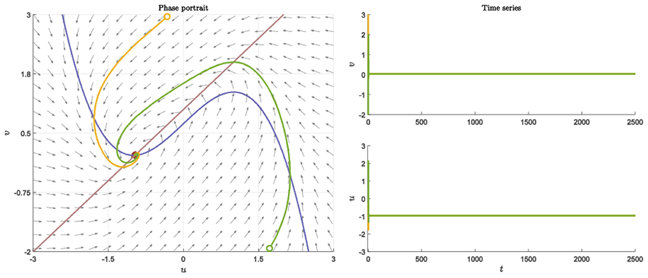
Figure 1. Nullcline, phase portraits with different initial value and time series when a = 1, b = 1, c = 2, d = 1, I = 0.7.

In this case, condition (H 2) becomes

$y={\Delta }_0+(a_{22}{D}_u+a_{11}{D}_v)({\Lambda }_{\alpha }^R+{\Lambda }_{\beta }^E)+D_u{D}_v{({\Lambda }_{\alpha }^R+{\Lambda }_{\beta }^E)}^2<0.$

Hence, Turing instability occurs in the general diffusion system when a₂₂D_u + a₁₁D_v > 0 and ${(a_{22}{D}_u+a_{11}{D}_v)}^2-4{\Delta }_0{D}_u{D}_v>0$. And the critical value is D_v = 8.3923 when D_u = 0.01 (Figure 2). Different dynamic behaviors [such as Hopf bifurcation (40) and chaos (41)] and various spatiotemporal patterns [such as irregular waves, target waves, traveling waves, and spiral waves (42, 43)] will appear when the system is subjected to different kinds and degrees of external stimulus. In the neural system, these spatiotemporal patterns are closely related to brain learning, memory, and information transmission. When the brain stores memory, the continuous firing rate of individual neurons shows a hierarchical change and the neurons show a strong temporal dynamic pattern and heterogeneity (33). Many factors contribute to the formation of short-term memory. Short-term memory does not form when the external stimulus is not sufficiently large (Figure 3). It is worth noting that neuronal activity is not only affected by external stimuli but also closely related to the interaction between nodes. The pattern remains flat when the external stimulus is large enough and the correlation degree of neurons is small. That is, short-term memory will not form (Figures 4A, B, 5A, B). When p increased to 0.01, neurons in the memory function areas fired, and the brain formed more vague memories (Figures 4C, D, 5C, D). Zheng et al. (37) found that neurons exhibit different pattern dynamics with the change of network connection probability p in the study of the HR model. This conclusion is also confirmed in the study of multilayer networks. Under the same degree of stimulation, if the number of neurons with the same functional attributes is different, the state of the neural network varies greatly (Figures 4B–D).

FIGURE 2

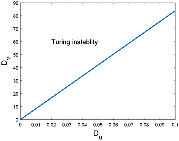
Figure 2. The range of Turing instability in the general diffusion system about D_u and D_v.

FIGURE 3

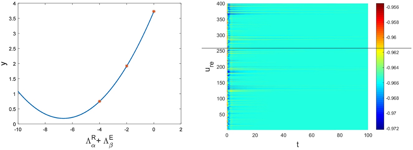
Figure 3. The relationship between ${\Lambda }_{\alpha }^R+{\Lambda }_{\beta }^E$ and y and the corresponding pattern when a = 1, b = 1, c = 2, d = 1, I = 0.7, D_u = 0.01, D_v = 8, p = 0.01. The red dots are the eigenvalues of the network Laplacian matrix.

FIGURE 4

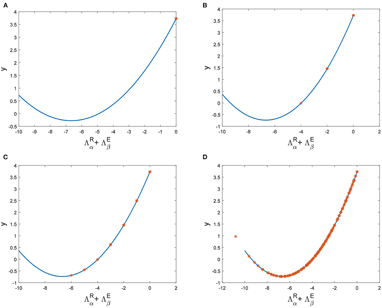
Figure 4. The relationship between ${\Lambda }_{\alpha }^R+{\Lambda }_{\beta }^E$ and y when a = 1, b = 1, c = 2, d = 1, I = 0.7, D_u = 0.01. (A) D_v = 9, p = 0.001. (B) D_v = 10, p = 0.006. (C) D_v = 10, p = 0.01. (D) D_v = 10, p = 0.1.

FIGURE 5

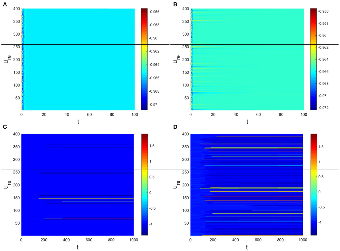
Figure 5. The corresponding Turing pattern in Figure 4. (A) D_v = 9, p = 0.001. (B) D_v = 10, p = 0.006. (C) D_v = 10, p = 0.01. (D) D_v = 10, p = 0.1.

The physiological environment in which neurons work is always full of noise. From the above analysis, we can see that when D_v = 9, p = 0.001 is taken, the neurons are always in resting state (Figure 5A). To investigate the robustness of noise to the current results, we add Gaussian white noise to the multilayer FHN network model. The noise intensity np about u is used as the control parameter. We find that the system is robust when np < O(10⁻⁵); when np > O(10⁻⁵), the neurons are excited and the short-term memory is vague (Figure 6).

FIGURE 6

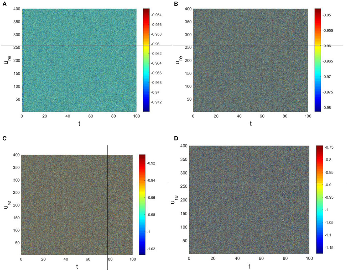
Figure 6. Pattern with a = 1, b = 1, c = 2, d = 1, I = 0.7, D_u = 0.01, D_v = 9, p = 0.001. (A) np = O(10⁻⁷). (B) np = O(10⁻⁶). (C) np = O(10⁻⁴). (D) np = O(10⁻³).

In the neural system, synapses can regulate the release of excitatory neurotransmitters of membrane potential or mediators through delayed feedback, so the response and transmission of signals will be delayed. Time delay affects the generation of bifurcation and phase synchronization between neurons, which affects the brain's memory function (27). Next, we explore the effect of time delay on neuronal activity. The transition of neurons from resting state to firing state is always accompanied by bifurcation behavior. Action potential exceeds the threshold when the time delay is greater than τ₀ = 0.5227, regardless of the influence of the network (Figure 7). c₁(0) = 0.021 − 0.2729ι, μ₂ = −0.021, β₂ = 0.042, T₂ = 0.162 can be found in Equation (27). Namely, the system generates subcritical Hopf bifurcation (similarly, we can get the supercritical Hopf bifurcation). From Figure 8, the network will affect the value of τ₀. In the study of the delayed neural network model, Zhao et al. (44) also found that the regulation of delay time can effectively control the formation of the pattern. Under the fixed network topology, the transmembrane current changes the membrane potential of neurons to different degrees with the increase of time delay. To more intuitively observe the collective behavior of neurons, we sorted 400 neuron nodes. When the delay time reaches 1, multiple neurons fire synchronously and participate in memory simultaneously (Figures 9A, B). It is found that the larger p is, the more obvious the synchronization phenomenon is (Figures 9B–D). Namely, short-term memory is relatively clear.

FIGURE 7

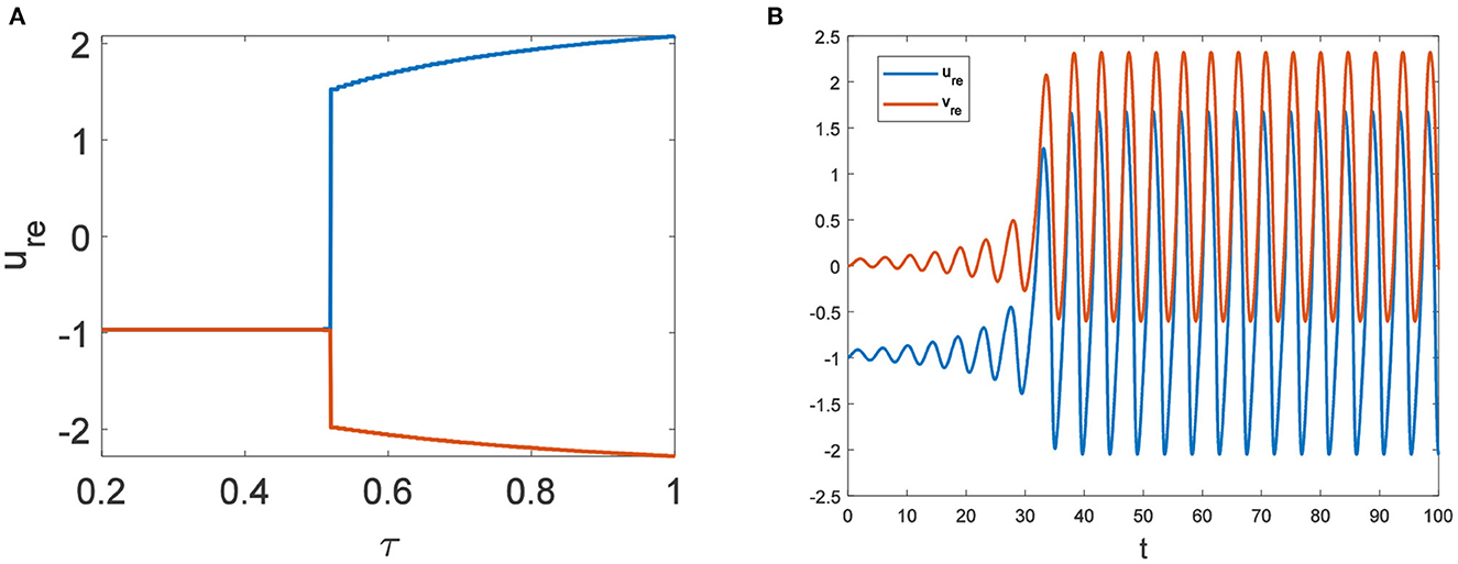
Figure 7. D_u = D_v = 0. (A) Bifurcation diagram about τ. The bifurcation point is τ = 0.5227. (B) The time series diagram with τ = 0.6.

FIGURE 8

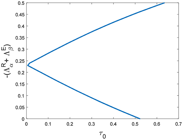
Figure 8. The relationship between τ₀ and eigenvalues of R□E.

FIGURE 9

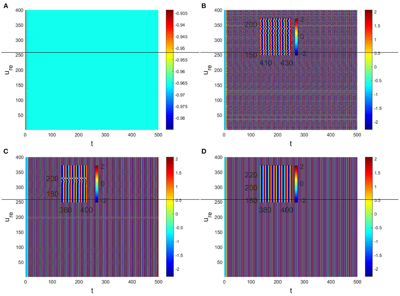
Figure 9. Pattern with D_u = 0.01, D_v = 8. (A) τ = 0.3, p = 0.01. (B) τ = 1, p = 0.01. (C) τ = 1, p = 0.1. (D) τ = 1, p = 0.3.

4. Conclusion

The brain is the most important organ in the human body, and its structure is very complex, so we have to simplify it when modeling. In this paper, we use the FHN model, which is simple but can describe the neuronal activity to explain the principle of short-term memory generation. The brain is a functional network that requires multiple neurons to work together for short-term memory. The brain regions responsible for specific tasks change their activity when the brain is storing memory (45). And pattern formation and selection can effectively detect collective behavior in excitable neural networks (27). Firstly, we establish the FHN model on the Cartesian product network and analyze the conditions of Turing instability. In the simulation, we found that short-term memory does not form when the probability of external stimulation and network connection is small. We test the robustness of the current results with Gaussian white noise and find that the system is robust when np < O(10⁻⁵). Short-term memory is formed when external stimuli, network connection probability, and noise reach a certain range. Because the pattern is not regular at this time, the short-term memory is blurred. Then we study the effect of time delay on short-term memory formation and find that short-term memory is formed when the delay time exceeds τ₀. Of course, neuronal activity is not only related to external stimuli but the topology of the network itself. When p and delay time reach a certain degree, the cluster dynamic behavior appear, and the pattern shows periodic phenomenon. At this time, the brain forms a relatively clear short-term memory. These results provide a new way to explain the principle of memory formation.

Data availability statement

The original contributions presented in the study are included in the article/supplementary material, further inquiries can be directed to the corresponding author.

Author contributions

JS made contributions to the conception or design of mathematical model, supervision, and funding acquistition. JW made contributions to writing, editing–original draft, and formal analysis. All authors contributed to the article and approved the submitted version.

Funding

This work was supported by National Natural Science Foundation of China (12272135) and Basic Research Project of Universities in Henan Province (21zx009).

Conflict of interest

The authors declare that the research was conducted in the absence of any commercial or financial relationships that could be construed as a potential conflict of interest.

Publisher's note

All claims expressed in this article are solely those of the authors and do not necessarily represent those of their affiliated organizations, or those of the publisher, the editors and the reviewers. Any product that may be evaluated in this article, or claim that may be made by its manufacturer, is not guaranteed or endorsed by the publisher.

References

1. Wang Q, Lu Q, Chen G, Duan L, et al. Bifurcation and synchronization of synaptically coupled FHN models with time delay. Chaos Solitons Fractals. (2009) 39:918–25. doi: 10.1016/j.chaos.2007.01.061

CrossRef Full Text | Google Scholar

2. Tehrani NF, Razvan M. Bifurcation structure of two coupled FHN neurons with delay. Math Biosci. (2015) 270:41–56. doi: 10.1016/j.mbs.2015.09.008

CrossRef Full Text | Google Scholar

3. Zhen B, Xu J. Fold-Hopf bifurcation analysis for a coupled FitzHugh-Nagumo neural system with time delay. Int J Bifurcat Chaos. (2010) 20:3919–34. doi: 10.1142/S0218127410028112

CrossRef Full Text | Google Scholar

4. Lin Y. Periodic oscillation analysis for a coupled FHN network model with delays. In: Abstract and Applied Analysis. Vol. 2013. Hindawi (2013).

Google Scholar

5. Han F, Zhen B, Du Y, Zheng Y, Wiercigroch M. Global Hopf bifurcation analysis of a six-dimensional FitzHugh-Nagumo neural network with delay by a synchronized scheme. Discrete Continuous Dyn Syst B. (2011) 16:457. doi: 10.3934/dcdsb.2011.16.457

CrossRef Full Text | Google Scholar

6. Yu D, Wang G, Ding Q, Li T, Jia Y. Effects of bounded noise and time delay on signal transmission in excitable neural networks. Chaos Solitons Fractals. (2022) 157:111929. doi: 10.1016/j.chaos.2022.111929

CrossRef Full Text | Google Scholar

7. Gan CB, Matjaz P, Qing-Yun W. Delay-aided stochastic multiresonances on scale-free FitzHugh-Nagumo neuronal networks. Chin Phys B. (2010) 19:040508. doi: 10.1088/1674-1056/19/4/040508

CrossRef Full Text | Google Scholar

8. Zeng C, Zeng C, Gong A, Nie L. Effect of time delay in FitzHugh-Nagumo neural model with correlations between multiplicative and additive noises. Physica A. (2010) 389:5117–27. doi: 10.1016/j.physa.2010.07.031

CrossRef Full Text | Google Scholar

9. Bashkirtseva I, Ryashko L. Analysis of excitability for the FitzHugh-Nagumo model via a stochastic sensitivity function technique. Phys Rev E. (2011) 83:061109. doi: 10.1103/PhysRevE.83.061109

CrossRef Full Text | Google Scholar

10. Rajagopal K, Jafari S, Moroz I, Karthikeyan A, Srinivasan A. Noise induced suppression of spiral waves in a hybrid FitzHugh-Nagumo neuron with discontinuous resetting. Chaos. (2021) 31:073117. doi: 10.1063/5.0059175

CrossRef Full Text | Google Scholar

11. Iqbal M, Rehan M, Hong KS. Robust adaptive synchronization of ring configured uncertain chaotic FitzHugh-Nagumo neurons under direction-dependent coupling. Front Neurorobot. (2018) 12:6. doi: 10.3389/fnbot.2018.00006

CrossRef Full Text | Google Scholar

12. Feng P, Wu Y, Zhang J. A route to chaotic behavior of single neuron exposed to external electromagnetic radiation. Front Comput Neurosci. (2017) 11:94. doi: 10.3389/fncom.2017.00094

CrossRef Full Text | Google Scholar

13. Liu H, Ge B. Turing instability of periodic solutions for the Gierer-Meinhardt model with cross-diffusion. Chaos Solitons Fractals. (2022) 155:111752. doi: 10.1016/j.chaos.2021.111752

CrossRef Full Text | Google Scholar

14. Ghorai S, Poria S. Turing patterns induced by cross-diffusion in a predator-prey system in presence of habitat complexity. Chaos Solitons Fractals. (2016) 91:421–9. doi: 10.1016/j.chaos.2016.07.003

CrossRef Full Text | Google Scholar

15. Lin J, Xu R, Li L. Turing-Hopf bifurcation of reaction-diffusion neural networks with leakage delay. Commun Nonlinear Sci Num Simulat. (2020) 85:105241. doi: 10.1016/j.cnsns.2020.105241

CrossRef Full Text | Google Scholar

16. Mondal A, Upadhyay RK, Mondal A, Sharma SK. Emergence of Turing patterns and dynamic visualization in excitable neuron model. Appl Math Comput. (2022) 423:127010. doi: 10.1016/j.amc.2022.127010

CrossRef Full Text | Google Scholar

17. Qu M, Zhang C. Turing instability and patterns of the FitzHugh-Nagumo model in square domain. J Appl Anal Comput. (2021) 11:1371–390. doi: 10.11948/20200182

CrossRef Full Text | Google Scholar

18. Zheng Q, Shen J. Turing instability induced by random network in FitzHugh-Nagumo model. Appl Math Computat. (2020) 381:125304. doi: 10.1016/j.amc.2020.125304

CrossRef Full Text | Google Scholar

19. Carletti T, Nakao H. Turing patterns in a network-reduced FitzHugh-Nagumo model. Phys Rev E. (2020) 101:022203. doi: 10.1103/PhysRevE.101.022203

CrossRef Full Text | Google Scholar

20. Lei L, Yang J. Patterns in coupled FitzHugh-Nagumo model on duplex networks. Chaos Solitons Fractals. (2021) 144:110692. doi: 10.1016/j.chaos.2021.110692

CrossRef Full Text | Google Scholar

21. Hu J, Zhu L. Turing pattern analysis of a reaction-diffusion rumor propagation system with time delay in both network and non-network environments. Chaos Solitons Fractals. (2021) 153:111542. doi: 10.1016/j.chaos.2021.111542

CrossRef Full Text | Google Scholar

22. Yang W, Zheng Q, Shen J, Hu Q, Voit EO. Pattern dynamics in a predator-prey model with diffusion network. Complex. (2022) 2022:9055480. doi: 10.1155/2022/9055480

CrossRef Full Text | Google Scholar

23. Ren Y, Sarkar A, Veltri P, Ay A, Dobra A, Kahveci T. Pattern discovery in multilayer networks. IEEE/ACM Trans Comput Biol Bioinform. (2021) 19:741–52. doi: 10.1109/TCBB.2021.3105001

CrossRef Full Text | Google Scholar

24. Asllani M, Busiello DM, Carletti T, Fanelli D, Planchon G. Turing instabilities on Cartesian product networks. Sci Rep. (2015) 5:1–10. doi: 10.1038/srep12927

CrossRef Full Text | Google Scholar

25. Tian C, Ruan S. Pattern formation and synchronism in an Allelopathic plankton model with delay in a network. SIAM J Appl Dyn Syst. (2019) 18:531–57. doi: 10.1137/18M1204966

CrossRef Full Text | Google Scholar

26. Chen Z, Zhao D, Ruan J. Delay induced Hopf bifurcation of small-world networks. Chin Ann Math B. (2007) 28:453–62. doi: 10.1007/s11401-005-0300-z

CrossRef Full Text | Google Scholar

27. Tang J. A review for dynamics of collective behaviors of network of neurons. Sci China Technol Sci. (2015) 58:2038–45. doi: 10.1007/s11431-015-5961-6

CrossRef Full Text | Google Scholar

28. Bullmore E, Sporns O. Complex brain networks: graph theoretical analysis of structural and functional systems. Nat Rev Neurosci. (2009) 10:186–98. doi: 10.1038/nrn2575

CrossRef Full Text | Google Scholar

29. Wang XJ. Synaptic reverberation underlying mnemonic persistent activity. Trends Neurosci. (2001) 24:455–63. doi: 10.1016/S0166-2236(00)01868-3

CrossRef Full Text | Google Scholar

30. Orhan AE, Ma WJ. A diverse range of factors affect the nature of neural representations underlying short-term memory. Nat Neurosci. (2019) 22:275–83. doi: 10.1038/s41593-018-0314-y

CrossRef Full Text | Google Scholar

31. Murray JD, Bernacchia A, Roy NA, Constantinidis C, Romo R, Wang XJ. Stable population coding for working memory coexists with heterogeneous neural dynamics in prefrontal cortex. Proc Natl Acad Sci USA. (2017) 114:394–9. doi: 10.1073/pnas.1619449114

CrossRef Full Text | Google Scholar

32. Bouchacourt F, Buschman TJ. A flexible model of working memory. Neuron. (2019) 103:147–60. doi: 10.1016/j.neuron.2019.04.020

CrossRef Full Text | Google Scholar

33. Goldman MS. Memory without feedback in a neural network. Neuron. (2009) 61:621–34. doi: 10.1016/j.neuron.2008.12.012

CrossRef Full Text | Google Scholar

34. Yao Y, Ma J. Weak periodic signal detection by sine-Wiener-noise-induced resonance in the FitzHugh-Nagumo neuron. Cogn Neurodyn. (2018) 12:343–9. doi: 10.1007/s11571-018-9475-3

CrossRef Full Text | Google Scholar

35. Yu D, Zhou X, Wang G, Ding Q, Li T, Jia Y. Effects of chaotic activity and time delay on signal transmission in FitzHugh-Nagumo neuronal system. Cogn Neurodyn. (2022) 16:887–97. doi: 10.1007/s11571-021-09743-5

CrossRef Full Text | Google Scholar

36. Zheng Q, Shen J, Xu Y. Spontaneous activity induced by gaussian noise in the network-organized fitzhugh-nagumo model. Neural Plasticity. (2020) 2020:6651441. doi: 10.1155/2020/6651441

CrossRef Full Text | Google Scholar

37. Zheng Q, Shen J, Zhang R, Guan L, Xu Y. Spatiotemporal patterns in a general networked hindmarsh-rose model. Front Physiol. (2022) 13:936982. doi: 10.3389/fphys.2022.936982

CrossRef Full Text | Google Scholar

38. Wang Z, Shi X. Electric activities of time-delay memristive neuron disturbed by Gaussian white noise. Cogn Neurodyn. (2020) 14:115–124. doi: 10.1007/s11571-019-09549-6

CrossRef Full Text | Google Scholar

39. Van Gorder RA. Turing and Benjamin-Feir instability mechanisms in non-autonomous systems. Proc R SocA. (2020) 476:20200003. doi: 10.1098/rspa.2020.0003

CrossRef Full Text | Google Scholar

40. Wouapi MK, Fotsin BH, Ngouonkadi EBM, Kemwoue FF, Njitacke ZT. Complex bifurcation analysis and synchronization optimal control for Hindmarsh-Rose neuron model under magnetic flow effect. Cogn Neurodyn. (2021) 15:315–47. doi: 10.1007/s11571-020-09606-5

CrossRef Full Text | Google Scholar

41. Yang W. Bifurcation and dynamics in double-delayed Chua circuits with periodic perturbation. Chin Phys B. (2022) 31:020201. doi: 10.1088/1674-1056/ac1e0b

CrossRef Full Text | Google Scholar

42. Rajagopal K, Ramadoss J, He S, Duraisamy P, Karthikeyan A. Obstacle induced spiral waves in a multilayered Huber-Braun (HB) neuron model. Cogn Neurodyn. (2022) 2022:1–15. doi: 10.1007/s11571-022-09785-3

CrossRef Full Text | Google Scholar

43. Kang Y, Chen Y, Fu Y, Wang Z, Chen G. Formation of spiral wave in Hodgkin-Huxley neuron networks with Gamma-distributed synaptic input. Commun Nonlinear Sci Num Simulat. (2020) 83:105112. doi: 10.1016/j.cnsns.2019.105112

CrossRef Full Text | Google Scholar

44. Zhao H, Huang X, Zhang X. Turing instability and pattern formation of neural networks with reaction-diffusion terms. Nonlinear Dyn. (2014) 76:115–124. doi: 10.1007/s11071-013-1114-2

CrossRef Full Text | Google Scholar

45. Baldassarre A, Lewis CM, Committeri G, Snyder AZ, Romani GL, Corbetta M. Individual variability in functional connectivity predicts performance of a perceptual task. Proc Natl Acad Sci USA. (2012) 109:3516–21. doi: 10.1073/pnas.1113148109

CrossRef Full Text | Google Scholar