Estimation of subjective quality of life in schizophrenic patients using speech features

1. Introduction

The number of psychiatric beds in Japan is much larger than in other countries, and the length of hospital stay is as long as 285 days (Italy: 13.9 days, U.K.: 42.3 days) (1). The Ministry of Health, Labour, and Welfare (MHLW) has announced a vision for reforming mental health and medical welfare in response to prolonged hospitalization. The MHLW vision fundamentally shifts its policy from inpatient care to community-based care. The vision clearly states the improvement of inpatient treatment, the improvement of patients' Quality of Life (QoL), and the development of support for early discharge from the hospital (2). Furthermore, a survey of readmission rates for 24,781 patients discharged in 2014 showed that 23% were re-admitted three months after discharge, 30% six months later, and 37% one year later (3). Prolonged hospitalization and high readmission rates are issues for psychiatric care in Japan.

QoL is an effective predictor of symptom remission and functional recovery among schizophrenic patients. As such, QoL is an essential measure of outcome in treatment (4, 5). It is crucial to understand and assess fluctuations in QoL scores and routine tests such as blood sampling; then use this information in interventions (6). However, QoL assessment is not routinely performed in clinical practice due to time constraints and lack of training and interest (7–9).

QoL can be divided into objective assessment and subjective assessment. This study focuses on subjective QoL because patients are the main actors in their lives during hospitalization and after discharge. The subjective assessment is possible because schizophrenic patients can feel and report social impairment (10). In addition, this study examined the use of voice input to estimate QoL status instead of the conventional self-administered and semi-constructed interview methods. Multi-lingual speech recognition and emotional speech recognition have been actively studied in recent years (11–13). Many voice-based applications have also been developed to remotely monitor the status and characteristics of speakers, such as health status (14–16). These latest developments motivate this study to consider speech recognition as a fast and efficient means of human-machine interaction (17).

Therefore, this study examined the estimation of subscale scores that measure the subjective QoL of schizophrenic patients using speech features as a simple method to measure QoL. The objectives were to (1) estimate the subscale scores from different patients or cross-sectional measurements, and (2) estimate the subscale scores from the same patient in different periods or longitudinal measurements. The proposed method allows schizophrenic patients to measure their subjective QoL by themselves in the future. Furthermore, the proposed method provides opportunities to monitor QoL continuously and regularly during hospitalization and after discharge. Patients and medical care providers can share data and analysis.

2. Material and methods

We examined the feasibility of estimating the subjective QoL of schizophrenic patients using speech features. The three subscale scores of the Japanese Schizophrenia Quality of Life Scale (JSQLS) were collected using a conversational agent. The conversational agent recorded the JSQLS responses and the audio of the conversation. Then, models were developed and compared to estimate the subscale scores. There were two kinds of models developed in this study.

1) Model development to estimate subscale scores from among different patients or cross-sectional measurements

2) Model development to estimate subscale scores from the same patient in different periods or longitudinal measurements

2.1. Target population demographics

Eighteen schizophrenic patients who agreed to participate in the study were included (Table 1). The mean age was 47.17 years, with seven males and 11 females. Global Assessment of Functioning (GAF) is a scale used to assess an overview of a subject's functioning. Psychological, social, and occupational functioning is rated as a single variable on an integer scale of 1–100 points (18). The rater evaluates the subject's condition according to the scale's rating criteria. For example, a 91–100 score indicates “very good functioning and no psychiatric symptoms.” Higher scores mean better symptoms and functioning. In this study, the psychiatrist or nurse in charge of the patient performed the evaluation (Table 2).

TABLE 1

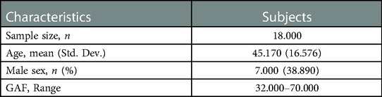
Table 1. Subjects’ demographics

TABLE 2

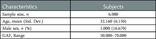
Table 2. Demographics of subjects measured twice.

2.2. SQLS as a measure of subjective QoL

JSQLS was used to measure subjective QoL. The JSQLS provides a subjective assessment of the impact of the disease on the subject's life. The JSQLS consists of three scales: Psychosocial (15 items), Motivation and Energy (7 items), and Symptoms and Side-effects (8 items). During the scale development in previous studies, the questions were selected based on in-depth patient interviews. Then, the JSQLS questions were examined for reliability and validity (18, 19).

2.2.1. JSQLS calculation method

This section describes how the three subscale scores are calculated and evaluated based on the subject's answers. There are five options for each question, and the score for each question ranges from 0 to 4 points.

“Always” (4 points)

“Often” (3 points)

“Sometimes” (2 points)

“Rarely” (1 point)

“Never” (0 points)

Each subscale was calculated to take values between 0 and 100, with higher scores indicating worse QoL while lower scores indicating better QoL.

$\begin{array}{rl}& \mathrm{Score}\mathrm{of}\mathrm{each}\mathrm{subscale}\\ & ={\displaystyle \frac{\mathrm{Sum}\mathrm{of}\mathrm{the}\mathrm{crude}\mathrm{scores}\mathrm{for}\mathrm{each}\mathrm{scale}}{4\times \mathrm{Number}\mathrm{of}\mathrm{questions}\mathrm{for}\mathrm{each}\mathrm{scale}}\times 100}\end{array}(1)$

On the one hand, the numerator is the total score based on each subject's choices. The denominator is calculated as 4 × 15 questions for “Psychosocial,” 4 × 7 questions for “Motivation and Energy,” and 4 × 8 questions for “Symptoms and Side-effects.” Note that four questions under “Motivation and Energy” are scored inversely, i.e., “Always” (0 points), “Often” (1 point), “Sometimes” (2 points), “Rarely” (3 points), and “never” (4 points).

2.3. Development of a conversational agent to measure subjective QoL

In this study, the conversational agent asked the patient 30 JSQLS questions and recorded the subject's voice as he or she answered each question (Figure 1).

FIGURE 1

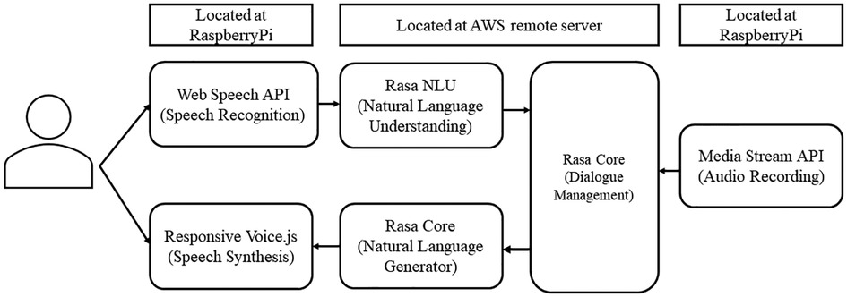
Figure 1. Conversational agent system architecture.

The Web Speech API converts the participant's speech into text. Then, the conversation agent uses natural language understanding to classify the answer choices (“Always,” “Often,” “Sometimes,” “Rarely,” and “Never”). Next, Rasa Core (20) manages the interaction, including the flow of conversation and context processing. Rasa Core's natural language generator selects appropriate text responses based on the context and flow of the conversation. Finally, ResponsiveVoice.js generates the spoken response from the text response.

2.4. Measurement method

Measurements were taken at the subject's hospital, a continuous employment support facility, and the subject's home. A quiet environment was ensured during the measurement for voice interaction and recording. First, the subjects were asked to read the 30 JSQLS questions before the measurement with the conversation agent. This step was implemented to prepare the subjects with the subsequent questions and clarify any questions. Then, the conversation agent spoke and displayed a question for the subject to listen and to see, respectively (Figure 2). Next, the subject answered back to the conversation agent. The conversation agent recorded the subject's response and audio using a microphone array. From this point, the conversation agent either (A) repeats the question if the subject's response is not understood or (B) proceeds to the next question until all 30 questions are finished (Figure 2).

FIGURE 2

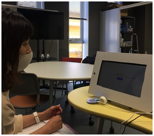
Figure 2. Preliminary experiment setup.

2.5. Audio processing and speech feature extraction

The following describes the acquired speech data. Subjects' speech was recorded at a sampling frequency of 48 kHz; the total unedited recording time, including conversational agent announcements, for the 18 subjects’ speech data was 98.200 min, with an average recording time of 5.456 min. The shortest recording time was 3.600 min and the longest was 10.917 min. The speech for the analysis was stripped of the conversational agent's announcements, silences, false responses, and noises. When the subject's speech was unclear, the conversation agent would listen back to the subject's speech, resulting in individual differences in recording time. The total recording time after removing the conversational agent's voice and the noise was 18.200 min, with an average duration of 1.011 min.

Using the Librosa audio library, speech data from 18 subjects were input, and Mel-spectrogram (128 dimensions), Mel-Frequency Cepstrum Coefficient (MFCC) (40 dimensions), and Chromagram (12 dimensions) speech features were Chromagram (12 dimensions) were extracted (Figure 3). A total of 3,240 speech features with 180 dimensions per subject and 18 subjects were used as the objective variables. Mel spectrogram and MFCC mimicked, to an extent, the natural sound frequency reception pattern of humans (13) and are often used for voice separation and classification (21). Chromagram can infer the vocal tract's resonance characteristics as the signal's energy distribution concerning saturation and time (22).

2.6. Model development

A model was developed using the extracted speech features to estimate the three JSQLS subscale scores. The features used to develop the model are the following.

FIGURE 3

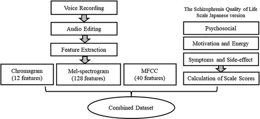
Figure 3. Data processing.

Let x be the explanatory variable and y. be the objective variable. Specifically,

$x_{1\sim 12}$: Chromagram

$x_{1\sim 128}$: Mel-spectrogram

$x_{1\sim 40}$: MFCC

$y_1$: “Psychosocial” subscale

$y_2$: “Motivation and Energy” subscale

$y_3$: “Symptoms and Side-effects” subscale

Python libraries like Pandas and Sklearn were used for data processing and model development. In this study, ten machine learning algorithms were utilized, and the errors of the trained models were compared. Ridge Regression, Lasso Regression, Elastic-Net Regression, k-Nearest Neighbors (k-NN), Decision Tree (DT), Support Vector Regression (SVR), Linear SVR (L.SVR), Random Forest (RF), Gradient Boosting (GB), and AdaBoost algorithms, were considered for developina model in estimating the subjective QoL of the subjects. Each algorithm is described below.

2.6.1. Ridge regression

Ridge Regression is a parameter estimation method used to address that addresses the collinearity problem frequently arising in multiple linear regression (23). Ridge Regression's coefficients minimize the sum of squared penalized residuals (24). L2 regularization is used in Ridge Regression.

$\underset{\omega }{\min }||X\omega -y|{|}_2^2+\alpha ||\omega |{|}_2^2$

2.6.2. Lasso regression

Lasso Regression minimizes the residual sum of squares subject to the sum of the absolute value of the coefficients being less than a constant. Because of the nature of this constraint, it tends to produce some coefficients that are exactly 0 and hence gives interpretable models (25). L1 regularization is used in Lasso Regression. The objective function to minimize is (26):

$\underset{w}{\min }{\displaystyle \frac{1}{2n_{\mathrm{samples}}}||Xw-y|{|}_2^2+\alpha ||w|{|}_1}(2)$

2.6.3. Elastic-Net regression

The Elastic-Net is particularly useful when the number of predictors (p) is much bigger than the number of observations (n). In contrast, the Lasso Regression does not have a satisfactory variable selection method to handle the p > n case. Therefore, Elastic-Net was proposed as an improved version of Lasso Regression to analyze high-dimensional data. The L1 part of the Elastic-Net performs automatic variable selection, while the L2 part stabilizes the solution paths. Hence, this method improves the prediction (27). The objective function to be minimized is (28):

$\underset{w}{\min }{\displaystyle \frac{1}{2n_{\mathrm{samples}}}||Xw-y|{|}_2^2+\alpha \rho ||w|{|}_1+{\displaystyle \frac{\alpha (1-\rho )}{2}}||w|{|}_2^2}(3)$

2.6.4. k-Nearest neighbors (k-NN)

k-NN algorithm for regression is a supervised learning approach. It predicts the target based on the similarity with other available cases. The similarity is calculated using the distance measure, with Euclidian distance being the most common approach. Predictions are made by finding the k most similar instances, i.e., the neighbors, of the testing point, from the entire dataset (29).

2.6.5. Decision tree (DT)

The Decision Trees algorithm is a non-parametric supervised learning method used for classification and regression.

In Decision Trees, a hierarchical tree structure consisting of Yes-No questions is learned. The disadvantage of decision trees is that they are prone to over-fitting and tend to be less versatile (30).

2.6.6. Support vector regression (SVR)

Instead of minimizing the observed training error, Support Vector Regression (SVR) attempts to minimize the generalization error bound to achieve generalized performance. SVR's concept is based on the computation of a linear regression function in a high-dimensional feature space where the input data are mapped via a nonlinear function (31).

2.6.7. Linear SVR (L.SVR)

Support Vector Regression (SVR) and Support Vector Classification (SVC) are time-consuming when using kernels. It has been demonstrated that Linear SVC and L. SVR generate models equivalent to kernel-SVR efficiently (32).

2.6.8. Random forest (RF)

Random Forest is one of the methods to deal with the problem of over-fitting to the training data in the DT algorithm. RFs consist of tree-structured classifiers {h ($\mathrm{x}$, $k$), $k$ = 1, …} where the {$k$} are identically independent distributed random vectors. Each tree cats a vote for the most popular class at input x (33).

2.6.9. Gradient boosting (GB)

The Gradient Boosting algorithm constructs additive regression models by sequentially fitting a simple parameterized function (base learner) to current “pseudo”-residuals by least squares at each iteration. The execution speed and approximation accuracy of GB can be greatly improved by incorporating randomization into the procedure (34).

2.6.10. Adaboost

Boosting is an approach to machine learning based on combining many relatively weak and i inaccurate rules to create a highly accurate prediction rule (35). The core principle of the AdaBoost regressor is to learn a sequence of weak regressors with high bias error but with low variance error. Repeatedly reweighted training instances are done based on the prediction error of each boosting iteration (36).

2.6.11. Nested cross-validation approach

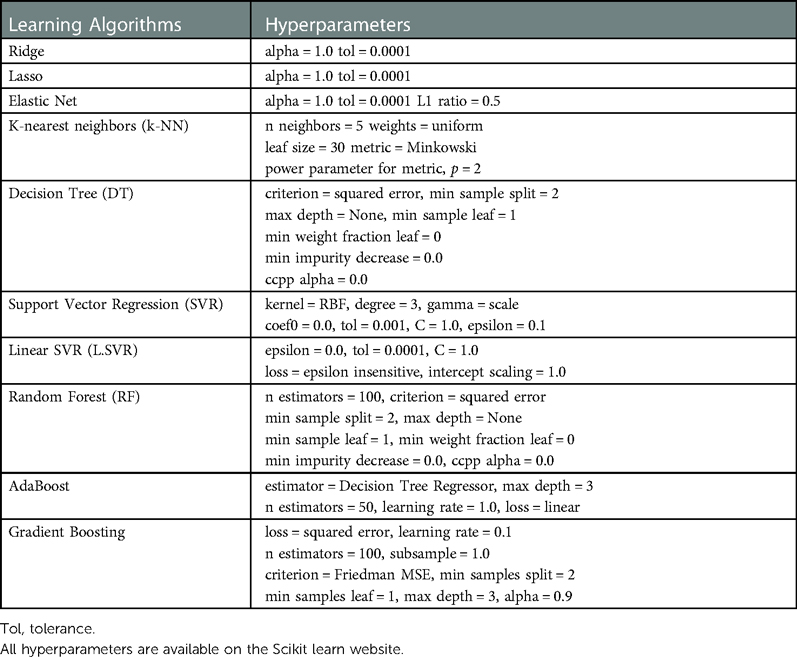
The Nested Cross-validation (CV) approach was used to compare machine learning algorithms on smaller subsets of the dataset (37) (Figure 4). Conventional CV uses the same data to compare different algorithms and evaluate the model's performance. The conventional CV approach leads to data leakage and over-fitting. On the other hand, the nested CV splits the data into training (①), validation (②), and test sets (③) multiple times. First, the outer loop divides the entire dataset into train and test sets. The outer loop is in charge of evaluating the model performance using the test set (③). Then, the inner loop divides the train set further into smaller training (①) and validation sets (②). In the inner loop, the best model was selected among the ten algorithms by comparing the average RMSE and MAE values. The Leave-One-Out method was used for partitioning the dataset. The default hyperparameters for each algorithm were kept during the entire model development. These default hyperparameters were provided in the Scikit learn library (see Appendix).

FIGURE 4

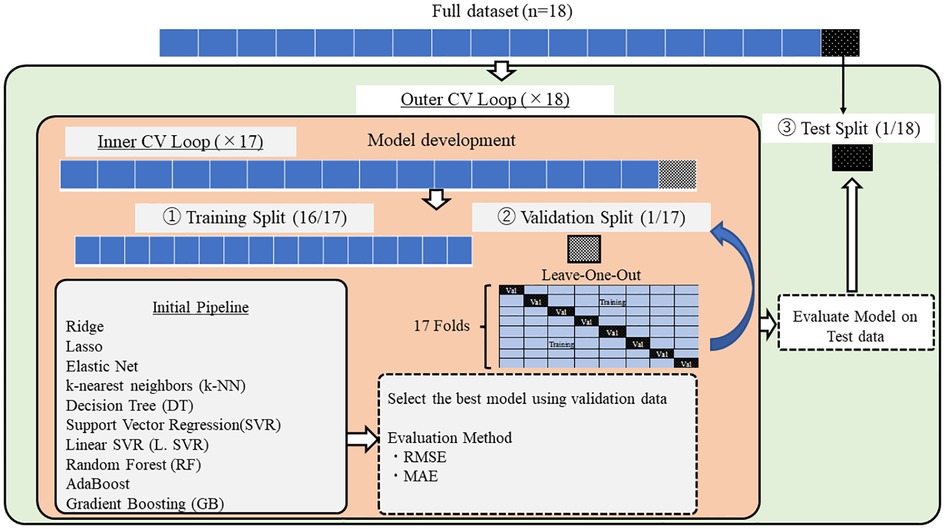
Figure 4. Model development.

For each of the ten algorithms, the error between ground truth and validation data was calculated using RMSE (Root Mean Squared Error) and MAE (Mean Absolute Error). RMSE is characterized by a strict evaluation of the error between the ground truth and the estimate using the squared form. The lower the RMSE is, the better the estimates of the model. On the other hand, MAE is the mean of the absolute difference between the ground truth and the estimated values. The lower the MAE is, the better the estimates of the model.

RMSE is computed as follows.

$RMSE=\sqrt{{\displaystyle \frac{1}{n}{\sum }_{i=0}^{n-1}{(y_i-\widehat{y_i})}^2}}(4)$

On the other hand, MAE is calculated as follows.

$MAE={\displaystyle \frac{1}{n}{\sum }_{i=1}^n|y_i-\widehat{y_i}|}(5)$

where n is the total number of data, $y_i$ is the actual value, ${\hat{y}}_i$ denotes the predicted value. Since this study estimates the subjective QoL thru three subscale scores, the average RMSE and MAE over these three subscale scores were also calculated. The average RMSE and MAE over three subscales were used during the model comparison.

2.7. Speech feature importance by SHAP value

In recent years, the interpretability of models has become more important than their accuracy. SHApley Additive exPlanations (SHAP) is a unified framework for interpreting predictions, allowing us to understand each feature's importance for the prediction (38).

Therefore, in this study, the SHAP value helps identify which of the three speech features contributes to the model.

2.8. Model development and evaluation to estimate scale scores from longitudinal measurements

QoL scores are inferred to change over time depending on the subject's condition. Therefore, we selected six subjects out of 18 subjects and conducted the second measurement after an average of 54.333 days (S.D. = 24.426). The data from the first 18 subjects were used as training data. For each of the ten models (using the same machine learning algorithm as in 2.6), the mean RMSE values for the three scales were compared using the validation data. The best model was used. Next, we evaluated the model using the scale scores of the six participants as unseen test data.

3. Results

This section describes the best models and evaluations of the ten algorithms selected for the cross-sectional and longitudinal measurements. Finally, we discuss the speech features that contributed to the model development.

3.1. Model comparison on validation set for cross-sectional measurement

First, the mean subscale scores among the 18 subjects (Table 3) were 45.000 for the “Psychosocial” subscale, 49.389 for the “Motivation and Energy” subscale, and 27.944 for the “Symptoms and Side-effects” subscale. These subscale scores were obtained from the subjects' JSQLS responses. The last subscale had the lowest score among the three subscales, which suggests that the subjects of this study had a good QoL concerning their symptoms and subsequent side effects. However, the minimum and maximum scores for the “Symptoms and Side Effects” scale were 0 and 78, respectively, indicating significant individual differences.

TABLE 3

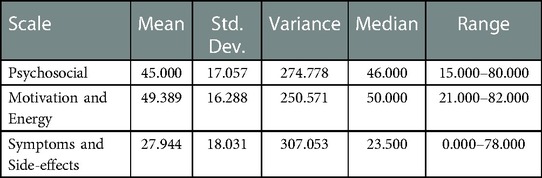
Table 3. RMSE and MAE scores for each scale on cross-sectional measurements.

Then, the ten algorithms were compared using the validation set produced in the inner loop. The mean RMSE and MAE values were calculated and ranked. With this method, the trained k-NN algorithm produced the lowest mean RMSE and MAE of 13.433 (SD = 10.206, n = 18). The average RMSE and MAE values for the validation data of the other models were in the following order (the mean values of RMSE and MAE are equal, and therefore one value is shown): SVR: 13.697, RF: 13.697, GB: 14.263, AdaBoost: 14.663, DT: 15.973, L.SVR: 21.466, Ridge: 21.496, ElasticNet: 25.976, Lasso: 28.975 (Table 4).

TABLE 4

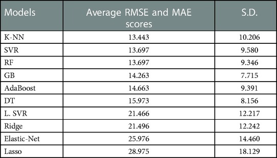
Table 4. The average RMSE and MAE values for the validation data.

3.2. Model comparison on test set for cross-sectional measurement

The selected best model (k-NN) was evaluated using the test set produced in the outer loop. The training resulted in a mean RMSE of 14.361 (SD = 0.674, n = 18) and a mean MAE of 10.9510 (SD = 0.6347, n = 18). The trained k-NN model produced a mean RMSE and MAE of 13.304 (SD = 10.392, n = 18) on the test set. The mean test RMSE was better than during training, and this observation can also be seen in 12 out of the 18 folds (Table 5).

TABLE 5

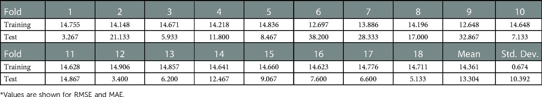
Table 5. Evaluation of training and test data with k-NN.

The RMSE and MAE for each subscale were 14.644 for “Psychosocial”, 13.633 for “Motivation and Energy”, and 11.633 for “Symptoms and Side-effects” (Table 6). The RMSE and MAE for “Symptoms and Side-effects” had the lowest values, but the minimum and maximum values were 1.200 and 51.800, respectively, which were larger than the other scales.

TABLE 6

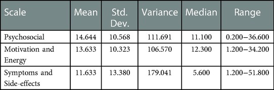
Table 6. RMSE and MAE scores for each subscale.

In each fold, RMSE and MAE were above 10 in 8 folds. Among them, fold 6 had the highest RMSE and MAE (38.200) and the highest scale scores (Psychosocial: 80, Motivation and Energy: 82, Symptoms and Side-effects: 78). Similarly, fold 9 had RMSE and MAE of 32.867 and lowest scale scores (Psychosocial: 15, Motivation and Energy: 21, Symptoms and side- effects: 0) (Table 7). There were 10 folds that could be estimated with RMSE and MAE less than 10. Among them, fold 1 had the lowest value of 3.267 (Table 8). The RMSE and MAE for each fold were then divided into two groups, above and less than 10, to determine whether there was a significant difference between the ground truth and the estimates for each group; for the group with RMSE and MAE above 10 (Figure 5A), “Psychosocial” p = 0.724, “Motivation and Energy” p = 0.724, and “Symptoms and Side-effects” p = 0.535. In the group with RMSE and MAE less than ten (Figure 5B), “Psychosocial” p = 0.724, “Motivation and Energy” p = 0.477, “Symptoms and Side-effects” p = 0.929. There were no statistically significant differences between the ground truth and the estimates.

FIGURE 5

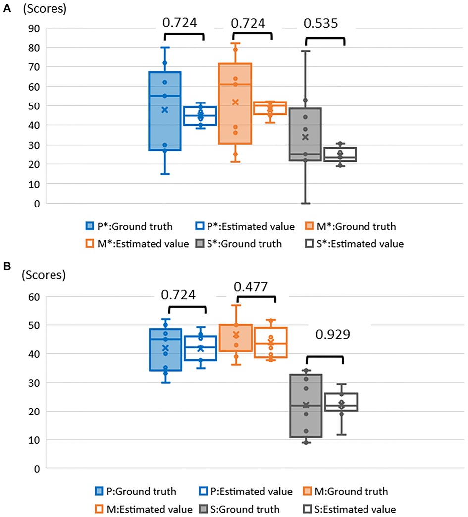
Figure 5. (A) Examination of significant differences between ground truth and estimates of RMSE and MAE above 10. *P, psychosocial; M, motivation and energy; S, symptoms and side–effects. (B) Examination of significant differences between ground truth and estimates of RMSE and MAE less than 10. *P, psychosocial; M, motivation and Energy; S, symptoms and side–effects.

TABLE 7

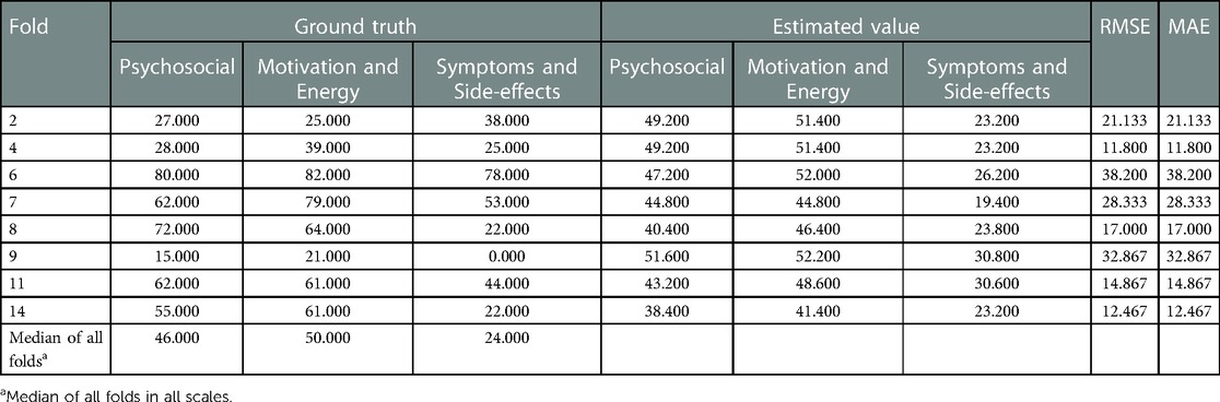
Table 7. Ground truth and estimated values for each subject with RMSE above 10.

TABLE 8

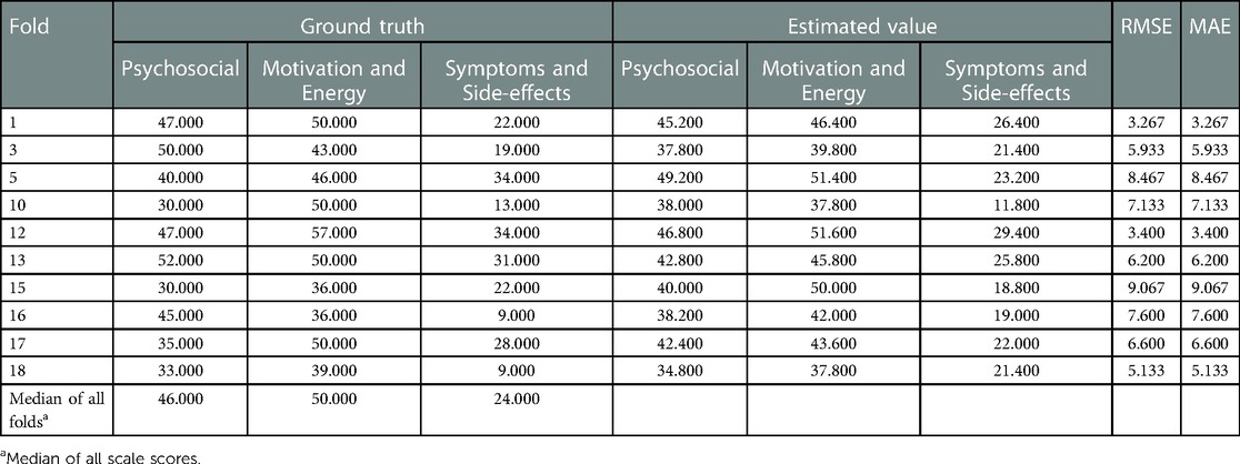
Table 8. Ground truth and estimated values for each subject with RMSE less than 10.

3.3. Model comparison on validation set for longitudinal (model to estimate scores for six longitudinal measurements)

First, the mean subscale scores among the six subjects were 46.500 for the “Psychosocial” subscale, 47.667 for the “Motivation and Energy” subscale, and 25.000 for the “Symptoms and Side-effects” subscale. Similar to the results of the first measurement, the scores on the “Symptoms and Side-effects” subscale were the lowest.

The models were developed using data from 18 subjects in order to estimate the scale scores for the 6 subjects. Ten algorithms were then compared using the validation set created in the inner loop. Mean RMSE and MAE values were computed and ranked. Thus, the trained RF algorithm produced the lowest mean RMSE and MAE of 13.301 (SD = 8.870, n = 18). The mean RMSE and MAE for the validation data of the other models were in the following order (mean RMSE and MAE are equal and represent a single value): k-NN: 13.304, SVR: 13.537, GB: 13.832, AdaBoost: 15.090, DT: 15.648, L. SVR: 20. 630, Ridge: 20.637, Elastic-Net: 26.105, Lasso: 30.787.

3.4. Model comparison on test set for longitudinal measurement

The RMSE and MAE for each subscale were 9.607 for the “Psychosocial” subscale, 4.767 for the “Motivation and Energy” subscale, and 9.508 for the “Symptoms and Side-effects” subscale (Table 9). The minimum and maximum values of RMSE and MAE for the “Psychosocial” subscale were 2.030 and 17.000, respectively, which were larger than the other scales.

TABLE 9

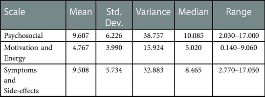
Table 9. RMSE and MAE scores for each scale on longitudinal measurements.

The results of the first and second measurements for the six subjects showed that the scores for each scale varied between −18 and +14 from the first measurement (Table 10). The RMSE and MAE values for each fold, five out of 6 folds, were less than 10. Fold 3 had the lowest RMSE and MAE at 4.557 and fold 2 had the highest at 13.540. The three subscales of Fold 2 remained high in the two measurements.

TABLE 10

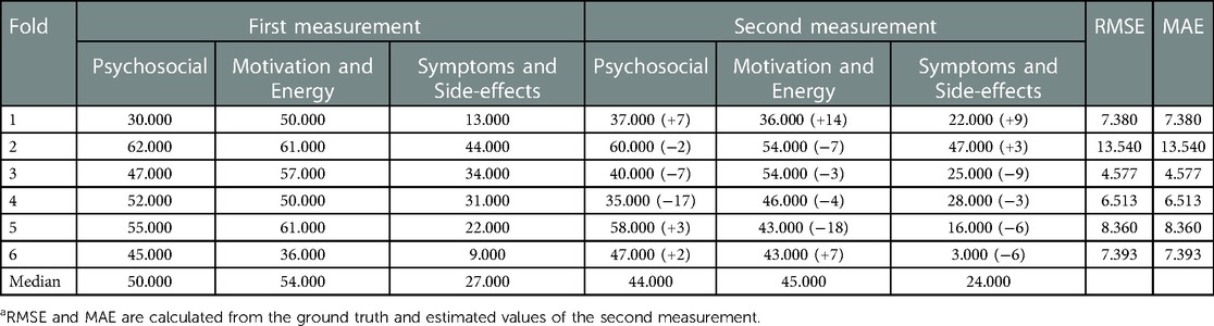
Table 10. First and second measurements (ground truth), and estimation scores^a from longitudinal measurements.

3.5. Speech feature importance to the estimation of scale scores

Speech features contributing to scoring estimation for each scale were identified by SHAP values. MFCC1 was selected as the most important speech feature for model development, followed by Mel-spectogram10.

4. Discussion

Scale score estimation results from cross-sectional and longitudinal measurements and the speech features that contributed to the model development will be discussed based on each result. Finally, we discussed the challenges and future work for this study.

4.1. Estimation of scale scores by cross-sectional measurement

Comparing the mean RMSE of the three scale scores among the ten algorithms, the k-NN was the best, with 13.433. The RMSE and MAE of the model with k-NN were 14.361 for the training data and 13.304 for the test data. Better test scores than the training suggest that the trained k-NN model could estimate the subscale scores on unseen subjects.

In each fold, the closer the ground truth was to the median, the lower the RMSE and MAE. On the other hand, 8 folds had RMSE and MAE above 10. Among them, fold6 had a high RMSE and MAE of 38.200 (Table 7). Subjects were unable to perform daily activities such as housework due to delusions. fold 9 had RMSE and MAE of 32.867. The subject was hospitalized in a psychiatric ward after the first measurement. In both cases, the scores of subjects who required the most medical intervention tended to deviate from the overall trend.

4.2. Estimation of scale scores by longitudinal measurement

Comparing the average RMSE of the three scale scores among the 10 algorithms, k-NN was the best with 13.301. The RMSE and MAE for the cross-sectional scales (“Psychosocial” 14.644, “Motivation, and Energy” 13.633, “Symptoms and Side-effects” 11.633) were above 10 for all subscales. However, the RMSE and MAE for the model with longitudinal measures were less than 10 for “Psychosocial” at 9.607, “Motivation and Energy” at 4.767, and “Symptoms and Side-effects” at 9.508.

In addition, in the model with cross-sectional measurement, 10 out of 18 folds had RMSE less than 10, while in the model with longitudinal measurement, 5 out of 6 folds had RMSE less than 10. In developing the model with the cross-sectional measurement, 1 fold was used as test data and 17 folds as training data. On the other hand, the longitudinal measurement used all data from 18 subjects as training data, which may be partly responsible for the increase in the number of training data.

4.3. Speech features that contributed to the estimation of scale scores

MFCC commonly contributed to the estimation of the scores of the three subscales. MFCC has many advantages, such as high discriminative power and noise immunity (39). Furthermore, MFCC can accurately characterize the vocal tract and accurately represent the phonemes produced by the vocal tract (40). The JSQLS response options are “Always,” “Often,” “Sometimes,” “Rarely,” and “Never”. Therefore, it would have been possible to use the vocalization patterns of the different choices for identification.

Finally, as issues and future perspectives of this study, the number of patients diagnosed with schizophrenia eligible to subjects was small at the collaborating institutions. Therefore, it is necessary to seek the participation of more subjects who use medical institutions and welfare services. In addition, the study found that the scores for “Symptoms and Side-effects” were the lowest among the subscales. The fact that the subjects in this study were not hospitalized patients may be a factor. Therefore, it is necessary to examine whether there is a difference in scores between hospitalized and non-hospitalized patients and to consider model building. Next, the model was developed using data from 18 subjects. Attempts were made to estimate six subjects' scale scores for the second measurement. The baseline of the scale scores differs depending on the individual conditions. Although only two measurements were used in this study, developing individual models based on continuous measurements may be helpful. In addition, it may be a more straightforward method to estimate subjective QoL by examining the possibility of estimating the scale scores using speech features of daily conversation with conversational agents (e.g., greetings).

A 3-year follow-up of schizophrenia patients in a previous study found that non-remitting patients had worse QoL and increased healthcare costs than remitting patients (41). The results of this study are considered a severe issue in psychiatric treatment in Japan, where the readmission rate is high and the length of hospital stay is extended. As one strategy, evaluating QoL using voice features enables continuous monitoring by applications and can be applied to telemedicine.

5. Conclusion

In this study, a model was developed to estimate the three scale scores of the Japanese Schizophrenia Quality of Life Scale (JSQLS) using speech features. The ten different machine learning algorithms were compared, with k-NN being the best. The RMSE of the training data was 14.361 and the MAE of the test data was 13.361, suggesting the generality of the model. In the estimation for scale scores on individual subjects, the RMSE and MAE were higher if the scale scores were far from the median. In this study, RMSE and MAE values were higher in subjects with psychiatric symptoms that interfered with daily life and in subjects hospitalized after the measurement. In the longitudinal measurement, a model was developed using data from 18 subjects, and scale scores were estimated for six subjects measured twice. The results showed that RF was the best, with RMSE and MAE less than ten in five of the 6 folds. The speech feature most involved in model development was MFCC, which may be the result of identifying speech patterns according to question choice. Future studies should analyze more data sets and consider model development based on longitudinal measurements of individuals.

Data availability statement

The original contributions presented in the study are included in the article/Supplementary Material. Further inquiries can be directed to the corresponding author.

Ethics statement

The studies involving human participants were reviewed and approved by Research Review Committee for Human Subjects of Kyushu Institution of Technology Graduate School of Life Science and Systems Engineering. Clinical Research Review Committee, University of Occupational and Environmental Health. The patients/participants provided their written informed consent to participate in this study.

Author contributions

YS, TN, NO, RY and TS: conceived the study. JNV: developed the conversational agent. YS, TN, and NO: selected the research subjects. YS, TN and JNV: collected the data. NO: supervised the data collection process. YS and JNV: processed and analyzed the data. YS: wrote and revised the manuscript. JNV and TS: provided feedback on the manuscript. RY and TS: reviewed and supervised the overall study progress. All authors contributed to the article and approved the submitted version.

Acknowledgments

Acknowledgments go to the subjects who participated and the staff at the facilities who assisted in data collection.

Conflict of interest

The authors declare that the research was conducted in the absence of any commercial or financial relationships that could be construed as a potential conflict of interest.

Publisher's note

All claims expressed in this article are solely those of the authors and do not necessarily represent those of their affiliated organizations, or those of the publisher, the editors and the reviewers. Any product that may be evaluated in this article, or claim that may be made by its manufacturer, is not guaranteed or endorsed by the publisher.

References

1. Ministry of Health, Labor and Welfare. Summary of 2020 Patient Survey (2020). Available at: https://www.mhlw.go.jp/toukei/saikin/hw/kanja/20/index.html (Accessed October 1, 2022).

2. Ministry of Health, Labour and Welfare. Vision for Reform of Mental Health and Medical Welfare (Summary) (2004). Available at: https://www.mhlw.go.jp/topics/2004/09/dl/tp0902-1a.pdf (Accessed October 1.2022).

3. Ministry of Health, Labor, and Welfare. Recent Trends in Mental Health and Medical Welfare Policy (2018). Available at: https://www.mhlw.go.jp/content/12200000/000462293.pdf (Accessed October 1, 2022).

4. Lambert M, Schimmelmann BG, Naber D, Eich FX, Schulz H, Huber CG, et al. Early- and delayed antipsychotic response and prediction of outcome in 528 severely impaired patients with schizophrenia treated with amisulpride. Pharmacopsychiatry. (2009) 42(6):77–83. doi: 10.1055/s-0029-1234105

CrossRef Full Text | Google Scholar

5. Hofer A, Baumgartner S, Edlinger M, Hummer M, Kemmler G, Rettenbacher MA, et al. Patient outcomes in schizophrenia I: correlates with sociodemographic variables, psychopathology, and side effects. Eur Psychiatry. (2005) 5–6:386–94. doi: 10.1016/j.eurpsy.2005.02.005

CrossRef Full Text | Google Scholar

6. Halyard MY, Frost MH, Dueck A, Sloan JA. Is the use of QOL data really any different than other medical testing? Curr Probl Cancer. (2006) 30(6):261–71. doi: 10.1016/j.currproblcancer.2006.08.004

PubMed Abstract | CrossRef Full Text | Google Scholar

7. Morris J, Perez D, McNoe B. The use of quality of life data in clinical practice. Qual Life Res. (1997) 7(1):85–91. doi: 10.1023/a:1008893007068

CrossRef Full Text | Google Scholar

8. Awad AG, Voruganti LN. Measuring quality of life in patients with schizophrenia: an update. Pharmacoeconomics. (2012) 30(3):183–95. doi: 10.2165/11594470-000000000-00000

PubMed Abstract | CrossRef Full Text | Google Scholar

9. Boyer L, Auquier P. The lack of impact of quality-of-life measures in schizophrenia: a shared responsibility? Pharmacoeconomics. (2012) 30(6):531–2. doi: 10.2165/11633640-000000000-00000

PubMed Abstract | CrossRef Full Text | Google Scholar

10. Skantze K, Malm U, Dencker SJ, May PR, Corrigan P. Comparison of quality of life with standard of living in schizophrenic out-patients. Br J Psychiatry. (1992) 161:797–801. doi: 10.1192/bjp.161.6.797

PubMed Abstract | CrossRef Full Text | Google Scholar

11. Narayanan A, Misra A, Sim KC, Pundak G, Tripathi A, Elfeky M, et al. Toward domain-invariant speech recognition via large scale training. (2018) IEEE spoken language technology workshop (SLT) (2018). doi: 10.1109/SLT.2018.8639610

12. Zeinali H, Burget L, Černocký JH. A multi purpose and large scale speech corpus in Persian and English for speaker and speech recognition: the DeepMine database. IEEE automatic speech recognition and understanding workshop (ASRU) (2019). p. 397–402. doi: 10.1109/ASRU46091.2019.9003882

13. Issa D, Demirci MF, Yazici A. Speech emotion recognition with deep convolutional neural networks. Biomed Signal Process Control. (2020) 59:1–11. doi: 10.1016/j.bspc.2020.101894

CrossRef Full Text | Google Scholar

14. Eyben F, Huber B, Marchi E, Schuller D, Schuller B. Real-time robust recognition of speakers’ emotions and characteristics on mobile platforms. International conference on affective computing and intelligent interaction (ACII) (2015). p. 778–80. doi: 10.1109/ACII.2015.7344658

15. Sandulescu V, Andrews S, Ellis D, Dobrescu R, Mozos OM. Mobile app for stress monitoring using voice features. The 5th conference on E-health and bioengineering (2015). doi: 10.1109/EHB.2015.7391411

16. Xu R, Mei G, Zhang G, Gao P, Judkins T, Cannizzaro M, et al. A voice-based automated system for PTSD screening and monitoring. Stud Health Technol Inform. (2012) 173:552–8. doi: 10.3233/978-1-61499-022-2-552

PubMed Abstract | CrossRef Full Text | Google Scholar

17. Ayadi ME, Kamel MS, Karray F. Survey on speech emotion recognition: features, classification schemes, and databases. Pattern Recogn. (2011) 44(3):572–87. doi: 10.1016/j.patcog.2010.09.020

CrossRef Full Text | Google Scholar

18. Kaneda Y, Imakura A, Ohmori T. The schizophrenia quality of life scale Japanese version (JSQLS). Clin Psychiatry. (2004) 46(7):737–9. doi: 10.11477/mf.1405100520

CrossRef Full Text | Google Scholar

19. Wilkinson G, Hesdon B, Wild D, Cookson R, Farina C, Sharma V. Self-report quality of life measure for people with schizophrenia: the SQLS. The Br J Psychiatry. (2000) 177(1):42–6. doi: 10.1192/bjp.177.1.42

PubMed Abstract | CrossRef Full Text | Google Scholar

20. Bocklisch T, Faulkner J, Pawlowski N, Nichol A. Rasa: open source language understanding and dialogue management. NIPS workshop on conversational AI (2017). doi: 10.48550/arXiv.1712.05181

21. Bartsch MA, Wakefield GH. Audio thumbnailing of popular music using chroma-based representations. IEEE Trans Multimedia. (2005) 7(1):96–104. doi: 10.1109/TMM.2004.840597

CrossRef Full Text | Google Scholar

22. Wakefield GH. Chromagram visualization of the singing voice. Models and analysis of vocal emissions for biomedical applications. Florence: Firenze University Press (1999). p. 24–9.

23. McDonald GC. Ridge regression. WIRE Comp Stats. (2009) 1(1):93–100. doi: 10.1002/wics.14

CrossRef Full Text | Google Scholar

24. Scikit learn. 1.1.2. Ridge regression and classification (2022). Available at: https://scikit-learn.org/stable/modules/generated/sklearn.linear_model.Ridge.html (Accessed January 8, 2023).

25. Tibshirani R. Regression shrinkage and selection via the Lasso. J R Stat Soc. (1996) 58(1):267–88. doi: 10.1111/j.2517-6161.1996.tb02080.x

CrossRef Full Text | Google Scholar

26. Scikit learn. 1.1.3. Lasso (2022). Available at: https://scikit-learn.org/stable/modules/linear_model.html?highlight=ridge+regression#lasso (Accessed January 8, 2023).

27. Zou H, Hastie T. Regularization and variable selection via the elastic net. J R Stat Soc. (2005) 67(2):301–20. doi: 10.1111/j.1467-9868.2005.00503.x

CrossRef Full Text | Google Scholar

28. Scikit learn. 1.1.5. Elastic-Net (2022). Available at: https://scikit-learn.org/stable/modules/linear_model.html?highlight=ridge+regression#elastic-net (Accessed January 8, 2023).

29. Bajaj P, Ray R, Shedge S, Vidhate S, Shardoor S. Sales prediction using machine learning algorithms. Int Res J Eng Technol. (2020) 7(6):3619–25.

Google Scholar

30. Müller CA, Guido S. Introduction to machine learning with python a guide for data scientists. Sebastopol, CA: Japan: O’REILLY (2017). 70 p.

31. Basak D, Pal S, Patranabis DC. Support vector regression. Stat Comput. (2007) 11(10):203–24.

Google Scholar

32. Ho CH, Lin CJ. Large-scale linear support vector regression. J Mach Learn Res. (2012) 13(1):3323–48. doi: 10.5555/2503308.2503348

CrossRef Full Text | Google Scholar

33. Breiman L. Random forests. Mach Learn. (2001) 45:5–32. doi: 10.1023/A:1010933404324

CrossRef Full Text | Google Scholar

34. Schapire RE. Explaining AdaBoost. Empirical Inference. (2013):37–52. doi: 10.1007/978-3-642-41136-6_5

CrossRef Full Text | Google Scholar

35. Xiao C, Chen N, Hu C, Wang K, Gong J, Chen Z. Short and mid-term sea surface temperature prediction using time-series satellite data and LSTM-AdaBoost combination approach. Remote Sens Environ. (2019) 233:1–44. doi: 10.1016/j.rse.2019.111358

CrossRef Full Text | Google Scholar

36. Friedman JH. Stochastic gradient boosting. Comput Stat Data Anal. (2002) 38(4):367–78. doi: 10.1016/S0167-9473(01)00065-2

CrossRef Full Text | Google Scholar

37. Raschka S. Model evaluation, model selection, and algorithm selection in machine learning. arXiv. (2020):1–48. doi: 10.48550/arXiv.1811.12808

CrossRef Full Text | Google Scholar

38. Lundberg SM, Lee SI. A unified approach to interpreting model predictions. 31st international conference on neural information processing systems (2017). p. 4768–77

39. Milton A, Roy SS, Selvi ST. SVM scheme for speech emotion recognition using MFCC feature. Int J Comput Appl. (2013) 69(9):34–9. doi: 10.5120/11872-7667

CrossRef Full Text | Google Scholar

40. Abdulmajeed NQ, Khateeb BA, Mohammed MA. A review on voice pathology: taxonomy, diagnosis, medical procedures and detection techniques, open challenges, limitations, and recommendations for future directions. J Intell Syst. (2022) 31(1):855–75. doi: 10.1515/jisys-2022-0058

CrossRef Full Text | Google Scholar

41. Haynes VS, Zhu B, Stauffer VL, Kinon BJ, Stensland MD, Xu L. Long-term healthcare costs and functional outcomes associated with lack of remission in schizophrenia: a post-hoc analysis of a prospective observational study. BMC Psychiatry. (2012) 12:1–10. doi: 10.1186/1471-244X-12-222

PubMed Abstract | CrossRef Full Text | Google Scholar

APPENDIX Hyperparameters used in model development

.