Membrane equilibration for in situ dissolved gas instrumentation: a comparison of four approaches

Many in situ dissolved gas instruments use a membrane inlet to extract gas from water enabling measurement in the gas phase. However, mass transport across membranes is slow, making it difficult to build instruments with fast time responses. Several approaches exist to improve time response, including pulling vacuum to enhance gas flux, but the trade-offs between different approaches are unclear. Starting from first principles, we present a set of analytical models describing the operation of four different approaches for operating a membrane-based dissolved gas instrument. Using these models, we obtain the steady state and dynamic performance characteristics of each approach, and identify design trade-offs between speed, sensitivity, and complexity. Insights from these models enable physics-based design decisions and design optimization instead of instrument designers needing to rely on empirical methods.

1 Introduction

As the ocean changes in response to anthropogenic influences, it is important to understand the impacts on the cycling and distribution of dissolved gases such as oxygen (O₂), carbon dioxide (CO₂) and methane (CH₄) Talley et al. (2016), Halpern et al. (2019), Hopkins et al. (2020), Levin (2018), Doney et al. (2009), Reay et al. (2018). Warmer ocean temperatures lead to larger deoxygenated zones, which impact ecosystems, and rising carbon dioxide levels lead to ocean acidification, which impacts ocean ecosystem health Levin (2018), Doney et al. (2009). To monitor dissolved gases, researchers use a combination of discrete bottle samples and in situ instrumentation. These measurements enable the observation of changing conditions over time, as well as model ground-truthing, which can lead to the prediction of future changes Takahashi et al. (2002), Talley et al. (2016), Wanninkhof et al. (2013).

Many techniques for measuring dissolved gases in situ involve using an equilibrator to extract gas from water, for analysis by gas phase instrumentation. Several reviews have compared equilibrator styles (Santos et al., 2012; Yoon et al., 2016; Webb et al., 2016), but most use direct air-water contact, which can only be used for surface measurements. For deep-sea applications, the only equilibrator style available is a membrane inlet, which uses a nonporous gas-permeable polymer membrane, supported mechanically to withstand hydrostatic pressure, to isolate water from an internal gas volume. Unfortunately, gas transport through nonporous membranes is slow, because of the solution-diffusion mechanism for mass transport through the polymer. Membrane inlets have been used successfully for a variety of deep-sea dissolved gas instruments (Tortell, 2005; McNeil et al., 2006; Bell et al., 2007; Wankel et al., 2010, Wankel et al., 2011, Wankel et al., 2013; Fietzek et al., 2014; Reed et al., 2018; Michel et al., 2018; Grilli et al., 2018).

Overcoming the low gas transport rate is a significant design challenge for deep-sea dissolved gas instrumentation. Several approaches have been used to improve time response, such as minimizing the internal gas volume (McNeil et al., 2006; Reed et al., 2018; Fietzek et al., 2014), pulling a vacuum (Tortell, 2005; Bell et al., 2007; Wankel et al., 2010; Wankel et al., 2011), or using a sweep gas (Grilli et al., 2018). While these approaches have been demonstrated in the field, the trade-offs between different design choices are not readily apparent. To the authors’ knowledge, the analytical tools to understand different membrane equilibration approaches are not available in the literature, making it impossible to make physics-informed design decisions. Here, we aim to fill this gap by deriving analytical models to describe membrane equilibration from first principles, and use those models to derive design rules and identify trade-offs. The goal is to provide the tools needed for future instrument developers to make more physics-informed design decisions.

We consider four approaches, or “operation modes”: (1) passive equilibration, where a fixed volume of gas is allowed to fully equilibrate with a flow of seawater, (2) active equilibration, where a vacuum is continuously pulled on the gas side of the membrane, (3) hybrid equilibration, a balance between passive and active where a vacuum is periodically pulled and released, and finally (4) exchange equilibration, where a fixed volume of water is allowed to equilibrate with a fixed volume of gas. Passive equilibration is used by many instruments reported in the literature [e.g., Reed et al. (2018) or Fietzek et al. (2014)]. Underwater mass spectrometers continuously pull a vacuum to extract gas and can achieve rapid time responses Chua et al. (2016), although the exact instrument control dynamics may differ from the dynamics derived here. The CADICA instrument, presented by Bass et al. (2012), uses exchange equilibration: it monitors total dissolved inorganic carbon (DIC) by acidifying and degassing an aliquot of water and monitoring the carbon dioxide in a fixed gas volume. Here, we introduce a new method, hybrid equilibration, that balances the trade-offs between passive and active equilibration.

In this work, analytical models are derived for different equilibration methods for membrane inlet dissolved gas instrumentation. Supplementary Material S1 lists all of the nomenclature used throughout this paper. We then use these models to understand the advantages, limitations, and design space for each method. We begin by deriving differential equations describing the dynamics of each method, then solve these for their steady state and step responses. Design relationships are called out to aid future instrument development, such as the dependence of time response on internal volume and the trade-off between sensitivity and speed. The resulting analytical models should also aid in future instrument designs, as they offer a way to parameterize expected ranges in the internal gas volume, allowing for informed design decisions for the instrumentation to measure composition of the equilibrated gas. With the analytical models and results, the instrument designer and field-going scientist will be able to make more informed design, calibration, and deployment decisions.

2 Background theory

Chemical potential gradients drive the mass transport of gases in membrane applications, and the chemical potential is continuous at material interfaces, such as the water-membrane and gas-membrane interface Wijmans and Baker (1995), Baker (2004), Nagy (2019); Cussler (2009), Wijmans and Baker (2006). We can model the transport across a membrane inlet by considering it as a series of “layers”: (1) a well-mixed water layer, (2) a water-side stagnant boundary layer, (3) a solid, nonporous polymer membrane, (4) porous membrane support structure(s), (5) a gas-side stagnant boundary layer, (6) and a well-mixed gas layer. At each interfacial transition, such as the water-membrane interface, the chemical potential is continuous, and constitutive equations like Henry’s Law and the ideal gas law can be used to relate the chemical potential to gas partial pressures (Wijmans and Baker, 1995; Baker, 2004; Nagy, 2019; Cussler, 2009; Wijmans and Baker, 2006). In this dissolved gas monitoring application, we seek to make measurements of the partial pressure of gas in the well-mixed gas layer, $P_g$ to infer the partial pressure of gas in the well-mixed water layer, $P_w$. We use a lumped-parameter model to describe the mass transport across the overall membrane inlet:

$J=k_{\mathit{eff}}\left(P_w-P_g\right)(1)$

where $J$ is the flux of an individual gas (e.g., CO₂) from the water-side to the gas-side of the membrane inlet and $k_{\mathit{eff}}$ is an effective mass transport coefficient. The total gas flux across the membrane inlet can be computed by adding up the fluxes of each individual gas. To use this lumped-parameter model, we must make the assumption that the timescales of changes to the overall system (e.g., equilibration of the instrument), are much slower than the timescales of changes within each “layer” (e.g., concentration within the membrane itself) Nagy (2019); Cussler (2009); Baker (2004). From Equation 1, it is clear that gas flux can be increased by minimizing $P_g$. This can be done by pulling a vacuum, using a sweep gas, or otherwise scrubbing the gas of interest.

The effective mass transport coefficient (Equation 1) can be computed using a resistance in series model Baker (2004), Nagy (2019), Wijmans et al. (1996):

$\frac{1}{k_{\mathit{eff}}}=\frac{1}{k_{bl}}+\frac{1}{k_m}(2)$

where $k_m$ is the mass transport coefficient for the membrane and $k_{bl}$ is the mass transport coefficient for the stagnant boundary layer. We neglect the mass transport resistances on the gas-side of the membrane due to the significant differences in diffusivity in gas versus water, but could be included as an additional term if warranted (e.g., if long tubing is used to connect the membrane to the internal gas volume).

The mass transport coefficient for the membrane can be expressed in terms of the membrane thickness, ${\delta }_m$ and the membrane permeability, $\mathbb{P}$, or equivalently with the solubility, $S_m$ and diffusivity, $D_m$, of the gas in the membrane material (Nagy, 2019; Wijmans and Baker, 2006; Baker, 2004):

$k_m=\frac{\mathbb{P}}{{\delta }_m}=\frac{S_m{D}_m}{{\delta }_m}(3)$

Similarly, mass transport coefficient within the stagnant boundary layer can be expressed as:

$k_{bl}=\frac{D_w{K}_H}{{\delta }_{bl}}(4)$

where $D_w$ is the diffusivity of the gas in water, $K_H$ is the solubility of the gas in water, and ${\delta }_{bl}$ is the thickness of the stagnant boundary layer (Sarmiento and Gruber, 2006; Cussler, 2009; Nagy, 2019). Many fields use mass transport coefficients with different variable naming conventions, so care is required to ensure the continuity of chemical potential and match units.

Considering Equations 2-4, the stagnant boundary layer can be thought of as second “membrane”, with effective permeability equal to the product of the diffusivity and solubility of the gas in water. If flow speed is increased significantly, eventually the stagnant boundary layer will be very thin, both through the increase in flow velocity and the triggering of turbulence. In this case, mass transfer resistance due to the stagnant boundary layer may be negligible. Once the flow has reached a point where the stagnant boundary layer can be ignored, the “best” possible mass transport has been reached, and increasing flow rate after this point will not appreciably impact the instrument response.

3 Operational modes

We compare four operational modes for an underwater membrane-equilibrated dissolved gas instrument (Figure 1). In all modes, gas-side instrumentation (e.g., a laser spectrometer) is used to monitor the partial pressure of gas(es) inside an internal gas volume, with the overall goal of using those measurements to estimate the water-side partial pressure(s). The four modes are:

1. Passive Equilibration, where a fixed volume of gas is allowed to equilibrate with flowing water.

2. Active Equilibration, where a vacuum pump is used to maintain a constant low pressure in the internal gas volume. The gas flux through the membrane inlet is increased because the partial pressures of each gas inside are nearly zero.

3. Hybrid Equilibration, where a vacuum pump is used intermittently to reduce the pressure, allowing the system to equilibrate passively when the vacuum pump is off. Hybrid equilibration therefore strikes a balance between active and passive equilibration.

4. Exchange Equilibration, where a fixed volume of water is allowed to equilibrate with the fixed volume of gas. Exchange equilibration is an automated sample analysis method, and a pump would flush the external water volume in between samples. In practice, mechanical mixing of the water is required to ensure a reasonable time response.

Figure 1

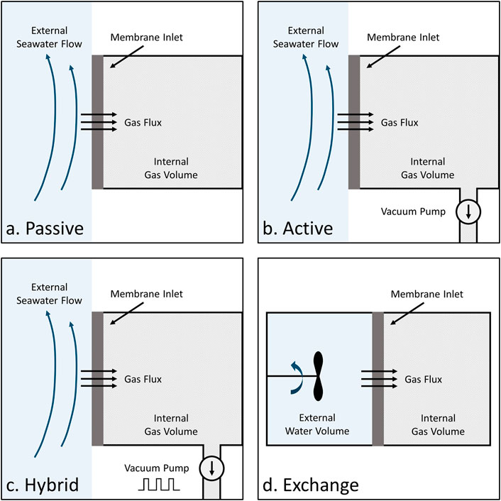
Figure 1. Four operational modes are considered: (a) Passive equilibration, where an internal gas volume equilibrates fully with a flow of seawater. (b) Active equilibration, where a vacuum pump continuously removes gas from the internal volume to maintain constant pressure. (c) Hybrid equilibration, where a vacuum pump periodically removes gas from the internal volume. The square wave symbol indicates that the vacuum pump is duty cycled. (d) Exchange equilibration, where a fixed volume of water is allowed to equilibrate with the internal gas volume. A mixer is required in practice to keep the water side well-mixed.

4 Evaluation methodology

The performance of each equilibration mode was assessed to provide insight into their theoretical performance characteristics and to guide future designs. First, the differential equations describing dynamics of each mode were derived starting from first principles using a mass balance approach. Key assumptions used in the derivations are listed in Supplementary Section S2. Then, where possible, the differential equations were solved analytically for the steady state and step responses. A computational approach was used for equilibration modes where a direct solution of the differential equations was not straightforward. Finally, design insights were drawn from the analytical results, leading to conclusions about optimization for each mode.

Membrane properties and dissolved gas conditions were chosen to simulate oceanographic conditions and are provided in the Supplementary Section S3. Representative operational settings (e.g., vacuum level) used for the four methods are also provided. Computations were performed using MATLAB 2020a.

5 Mathematical derivations

5.1 Passive equilibration

5.1.1 Differential equations

Under passive equilibration, the mass balance for the gas volume is:

$\frac{d{n}_g}{dt}=A{k}_{\mathit{eff}}\left(P_w-P_g\right)(5)$

where $n_g$ is the total number of moles of an individual gas on the gas-side of the membrane and $A$ is the area of the membrane. Using the ideal gas law, differentiated under constant temperature, Equation 5 can be rewritten:

$\frac{d{P}_g}{dt}=\frac{k_{eff}AR{T}_g}{{\forall }_g}(P_w-P_g)(6)$

where $R$ is the universal gas constant, $T_g$ is the temperature of the gas, and ${\forall }_g$ is the gas volume. We can define a characteristic time for gas equilibration, ${\tau }_g$:

${\tau }_g=\frac{{\forall }_g}{k_{eff}AR{T}_g}(7)$

Substituting Equation 7 into Equation 6 to remove ${\tau }_g$ results in the differential equation for passive equilibration:

$\frac{d{P}_g}{dt}=\frac{1}{{\tau }_g}\left(P_w-P_g\right)(8)$

The dynamics are independent of changes in other gases.

5.1.2 Steady state response

The solution to Equation 8 at steady state is: $P_g=P_w$. Provided enough time is allowed for the system to reach steady state, measurements of partial pressure in the gas volume equal the partial pressure in the water. This feature is one of the main advantages of passive equilibration.

5.1.3 Step response

The step response of Equation 8 is:

$P_g\left(t\right)=\left(P_{g,0}-P_w\right)e^{-t/{\tau }_g}+P_w(9)$

Therefore, when subjected to varying water-side partial pressures, passive equilibration acts like a low-pass filter.

5.2 Active equilibration

5.2.1 Differential equations

Under active equilibration, the vacuum pump is controlled to maintain a constant total pressure, $P_{\mathit{tot}}$. Therefore, the total molar flux through the membrane must be balanced by the vacuum pump. The molar flow through the vacuum pump, ${\dot{n}}_{\mathit{vac}}$, can be expressed:

${\dot{n}}_{\mathit{vac}}={\displaystyle \sum _{q=1}^y}A{k}_{\mathit{eff,q}}\left(P_{w,q}-P_{g,q}\right)(10)$

where the summation adds up the flow of each individual gas through the membrane, for $y$ total gases.

The mass balance for an individual gas can be written in terms of the flow across the membrane and the flow through the vacuum pump. We assume the vacuum pump removes gas independently of gas type (i.e., it is not selective). Therefore, the molar flow through the vacuum pump is proportional to the concentration of the gas, $X_i$. For active equilibration we use the subscript $i$ to indicate the gas of interest, since ${\dot{n}}_{\mathit{vac}}$ depends on all gases. The mass balance for a single gas is then:

$\frac{d{n}_{g,i}}{dt}=A{k}_{\mathit{eff,i}}\left(P_{w,i}-P_{g,i}\right)-X_i{\dot{n}}_{\mathit{vac}}(11)$

Equation 11 can be rewritten in terms of partial pressures using the ideal gas law under constant temperature:

$\frac{d{P}_{g,i}}{dt}=\left(\frac{k_{eff,i}AR{T}_g}{{\forall }_g}\right)(P_{w,i}-P_{g,i})-P_{g,i}\frac{{\dot{n}}_{vac}}{n_{tot}}(12)$

where $n_{\mathit{tot}}$ is the total number of moles of gas. Equation 12 can be simplified by substituting

$\frac{d{P}_{g,i}}{dt}=\left(\frac{1}{{\tau }_{g,i}}\right)\left(P_{w,i}-P_{g,i}\right)-P_{g,i}\frac{{\dot{n}}_{\mathit{vac}}}{n_{\mathit{tot}}}(13)$

Equation 13 can be rewritten using the ideal gas law and Equation 10, and further simplified by recognizing the form of ${\tau }_{g,i}$:

$\frac{d{P}_{g,i}}{dt}=\left(\frac{1}{{\tau }_{g,i}}\right)\left(P_{w,i}-P_{g,i}\right)-\frac{P_{g,i}}{P_{\mathit{tot}}}{\displaystyle \sum _{q=1}^y}\left(\frac{1}{{\tau }_{g,q}}\right)\left(P_{w,q}-P_{g,q}\right)(14)$

where $P_{\mathit{tot}}$ is the total pressure. This is a set of $y$ nonlinear, coupled equations. The multiplicative terms in the summations (e.g., $P_{g,i}{P}_{g,q}$) introduce nonlinearity and couple the equations, making the dynamics more complex.

Alternatively, Equation 13 can be rewritten by defining a characteristic residence time, ${\tau }_{\mathit{res}}$:

${\tau }_{\mathit{res}}=\frac{n_{\mathit{tot}}}{{\dot{n}}_{\mathit{vac}}}(15)$

which results in:

$\frac{d{P}_{g,i}}{dt}=\left(\frac{1}{{\tau }_{g,i}}\right)\left(P_{w,i}-P_{g,i}\right)-\left(\frac{1}{{\tau }_{\mathit{res}}}\right)P_{g,i}(16)$

This form is easier to interpret analytically, but it is important to note that ${\tau }_{\mathit{res}}$ depends on all gases.

5.2.2 Steady state response

At steady state Equation 16 becomes:

$P_{w,i}=\left(1+\frac{{\tau }_{g,i}}{{\tau }_{\mathit{res}}}\right)P_{g,i}(17)$

Both ${\tau }_{g,i}$ and ${\tau }_{\mathit{res}}$ are required to estimate $P_{w,i}$ from measurements of $P_{g,i}$. Laboratory characterization could be used to estimate ${\tau }_{g,i}$ and its environmental sensitivities (e.g., temperature) a priori, but ${\tau }_{\mathit{res}}$ depends on all gases and cannot be constrained with laboratory experiments alone. Ignoring the dependence of ${\tau }_{\mathit{res}}$ on other gases, such as assuming ${\tau }_{\mathit{res}}$ = constant, leads to significant cross-sensitivity. Cross-sensitivity can be avoided by adding a mass flow meter to measure ${\dot{n}}_{\mathit{vac}}$ and compute ${\tau }_{\mathit{res}}$ using Equation 15.

5.2.3 Step response

It is difficult to solve for an arbitrary step response because the equations describing active equilibration are nonlinear and coupled (Equation 14). However, it is possible to solve for a step response to small perturbations around equilibrium, such that ${\dot{n}}_{\mathit{vac}}$ and ${\tau }_{\mathit{res}}$ are approximately constant. Equation 16 can be rewritten in the following form:

$\frac{d{P}_{g,i}}{dt}=\left(\frac{1}{{\tau }_{g,i}}\right)P_{w,i}-\left(\frac{1}{{\tau }_{g,i}}+\frac{1}{{\tau }_{\mathit{res}}}\right)P_{g,i}(18)$

We define the characteristic active equilibration time, ${\tau }_{\mathit{act,i}}$, as:

$\frac{1}{{\tau }_{\mathit{act,i}}}=\frac{1}{{\tau }_{g,i}}+\frac{1}{{\tau }_{\mathit{res}}}(19)$

Equation 19 can be rewritten as:

${\tau }_{\mathit{act,i}}=\frac{{\tau }_{\mathit{res}}{\tau }_{g,i}}{{\tau }_{g,i}+{\tau }_{\mathit{res}}}(20)$

Using Equation 20 we can rewrite Equation 18 in a form similar to the passive equilibration equations:

$\frac{d{P}_{g,i}}{dt}=\left(\frac{1}{{\tau }_{g,i}}\right)P_{w,i}-\left(\frac{1}{{\tau }_{\mathit{act,i}}}\right)P_{g,i}(21)$

The step response for Equation 21 is:

$P_{g,i}\left(t\right)=\left(P_{g,i,0}-\frac{{\tau }_{\mathit{act,i}}}{{\tau }_{g,i}}{P}_{w,i}\right)e^{-t/{\tau }_{\mathit{act,i}}}+\frac{{\tau }_{\mathit{act,i}}}{{\tau }_{g,i}}{P}_{w,i}(22)$

It can be shown algebraically that the steady state value $\left(P_{g,i}(\infty )=\frac{{\tau }_{\mathit{act,i}}}{{\tau }_{g,i}}{P}_{w,i}\right)$ is consistent with Equation 17.

5.3 Hybrid equilibration

5.3.1 Differential equations

Since hybrid equilibration alternates between an equilibration phase and vacuum phase, we consider the mass balance for each phase separately. During the equilibration phase, the mass balance is identical to passive equilibration, therefore the dynamics are also identical:

$\frac{d{P}_g}{dt}=\frac{1}{{\tau }_g}\left(P_w-P_g\right)0\le t\le t_e(23)$

where $t_e$ is the amount of time the instrument stays in the equilibration phase. We assume the time spent in the vacuum phase, $t_v$, is significantly less than the time spent in the equilibration phase $(t_v\ll t_e)$, which is possible with a suitably sized vacuum pump. With this assumption, flux during the vacuum phase can be neglected, allowing us to treat the concentration of each gas as constant during the vacuum phase. The gas dynamics during the vacuum phase can then be expressed:

$\frac{d{P}_g}{dt}=\frac{d{P}_{\mathit{tot}}}{dt}X\left(t_e\right)t_e<t\le t_e+t_v(24)$

where $\frac{d{P}_{\mathit{tot}}}{dt}$ is the rate at which the vacuum pump reduces the total pressure in the gas volume, and $X(t_e)$ is the concentration at the start of the vacuum phase. For simplicity, we treat $\frac{d{P}_{\mathit{tot}}}{dt}$ as constant.

Combining Equation 23 and Equation 24, we obtain a piece-wise description of the repeating hybrid equilibration cycle:

$\frac{d{P}_g}{dt}=\left\{\begin{array}{cc}\frac{1}{{\tau }_g}\left(P_w-P_g\right)\hfill & 0\le t\le t_e\hfill \\ \frac{d{P}_{\mathit{tot}}}{dt}X\left(t_e\right)\hfill & t_e<t\le t_e+t_v\hfill \end{array}\right.(25)$

At the start of the next cycle, the initial condition for $P_g$ is equal to the final value for $P_g$, i.e., $P_g(0,\mathrm{n}\mathrm{e}\mathrm{x}\mathrm{t})=P_g(t_e+t_v)=X(t_e)P_{\mathit{nom}}$.

5.3.2 Steady state response

An instrument using hybrid equilibration never reaches ‘true’ steady state ($d{P}_g/dt$ = 0), but will reach a state of dynamic equilibrium, where the equilibration cycle repeats with the same start and ending point. At dynamic equilibrium, the expressions for the cycle become:

$P_{g,i}=\left\{\begin{array}{cc}\left(P_g\left(0\right)-P_w\right)e^{-t/{\tau }_g}+P_w\hfill & 0\le t\le t_e\hfill \\ P_{\mathit{tot}}\left(t\right)X\left(t_e\right)\hfill & t_e<t<t_e+t_v\hfill \\ P_{\mathit{nom}}X\left(t_e\right)\hfill & t=t_e+t_v\hfill \end{array}\right.(26)$

At the start of the next cycle, $P_g(0)$ would equal $P_g(t_e+t_v)$. The step response portion of the cycle matches Equation 9.

Due to the piece-wise definition, it is difficult to make further conclusions analytically. To characterize the operation of hybrid equilibration at steady state, we used MATLAB to iterate through the equilibration cycle until a steady state was reached for different levels of $P_w$. The average value of the data from equilibration phase exactly matched the steady state value for active equilibration operating using a pressure setting equal to the average total pressure. In other words: on average, hybrid equilibration follows active equilibration.

Since hybrid equilibration operates in cycles, it requires more data processing steps to interpret the data. To obtain an estimate for $P_w$, the data from the equilibration time period is used. If the equilibration time is much shorter than the characteristic passive equilibration time $(t_e\ll {\tau }_g)$, we can use a Taylor Series expansion for the exponential term around $t=0$. Retaining the linear terms and rearranging, we find an equation for a line:

$P_g\left(t\right)\approx \left(\frac{P_w-P_g\left(0\right)}{{\tau }_g}\right)t+P_g\left(0\right)(27)$

We can recognize Equation 27 as a line in slope intercept form. If we define the slope, $m$, as:

$m=\frac{P_w-P_g\left(0\right)}{{\tau }_g}(28)$

We can use Equation 28 to rearrange Equation 27 to obtain an estimate for $P_w$:

$P_{w=}=m{\tau }_g+P_g\left(0\right)(29)$

If $t_e$ is not significantly less than ${\tau }_g$, a higher order approximation, or even the full exponential, could be used to fit the data.

Hybrid equilibration data can also be interpreted on a cycle-average basis. The average of measurements collected during each equilibration phase matches an equivalent active equilibration response. The total pressure rise during the equilibration phase corresponds to the total mass flux, so the data could be interpreted without cross-sensitivity using the active equilibration equations. The additional measurement of total gas flux into the instrument can be used to monitor for changes in instrument performance (e.g., membrane fouling) or detect changes in other gases (e.g., oxygen decrease).

When hybrid equilibration data is interpreted on either a cycle-by-cycle or cycle-average basis, the ‘oscillatory’ nature of the data is removed. Using the cycle-by-cycle interpretation (Equation 29), an instantaneous estimate for $P_w$ is produced. Using the cycle-average interpretation, the data follows the response of an equivalent active instrument, and must be interpreted using Equation 17 to obtain an estimate for $P_w$.

5.3.3 Step response

Due to the piece-wise definition, it is difficult to obtain a step response analytically. However, it is simple to iterate through the cycles computationally using Equation 26 if the step occurs during the vacuum phase or Equation 25 and the MATLAB function ode45 if the step input occurs at an arbitrary time. As with the computational solution for the steady state response, the hybrid equilibration response tracks the active equilibration response on average.

If the hybrid equilibration data is interpreted on a cycle-by-cycle basis, using the slope and intercept from each equilibration phase (Equation 29) to obtain an estimate for $P_g$, the resulting estimate is effectively ‘instantaneous’, and the data acts as if we were taking discrete measurements with an infinitely fast sensor. With a discrete sampling rate, the overall bandwidth of the measurement is described by the Nyquist theorem, and we can compute an effective timescale using this as the cutoff frequency.

An important difference between hybrid data and active data is that the data rate is necessarily much lower than an equivalent active instrument. This is because the data from each equilibration period is used to generate a single estimate of the water-side gas partial pressure. There is also a ‘lag’ associated with it: you must wait until a cycle is complete to interpret the data. These aspects could be a limitation in dynamic environments requiring real-time data interpretation.

5.4 Exchange equilibration

5.4.1 Differential equations

To derive the differential equations describing exchange equilibration, we consider a mass balance on both the water and gas side of the membrane. On the gas side, the conditions are identical to passive equilibration, so it follows the same mass balance (Equation 5) and differential equation (Equation 8). Since there are no leaks, the molar flow into the gas volume must equal the molar flow out of the water volume. Therefore, the mass balance on the water side is:

$\frac{d{n}_w}{dt}=-\frac{d{n}_g}{dt}=-A{k}_{\mathit{eff}}\left(P_w-P_g\right)(30)$

where $n_w$ is the number of moles of an individual gas dissolved on the water-side of the membrane. Then, substituting for $\frac{d{n}_w}{dt}$ using Henry’s Law differentiated under constant temperature and rearranging, Equation 30 becomes:

$\frac{d{P}_w}{dt}=\frac{A{k}_{eff}}{{\rho }_w{\forall }_w{K}_H}(P_g-P_w)(31)$

where ${\rho }_w$ is the density of the water. Similarly to passive equilibration, we can define a characteristic time for the equilibration of the water-side of the membrane, ${\tau }_w$:

${\tau }_w=\frac{{\rho }_w{\forall }_w{K}_H}{k_{eff}A}(32)$

After substituting Equation 32 into Equation 31, the result is a set of coupled linear differential equations describing the gas dynamics on both sides of the membrane:

$\begin{array}{cc}\hfill \frac{d{P}_g}{dt}& =\frac{1}{{\tau }_g}\left(P_w-P_g\right)\hfill \\ \hfill \frac{d{P}_w}{dt}& =\frac{1}{{\tau }_w}\left(P_g-P_w\right)\hfill \end{array}(33)$

Changes on one side of the membrane reflect changes on the other.

5.4.2 Steady state response

At steady state, the molar flux across the membrane will be zero, and $P_g=P_w$. It is easiest to solve for the steady state partial pressure, $P_{\infty }=P_g(t=\infty )=P_w(t=\infty )$, by considering the fact that the total number of moles in the system consisting of both the water and gas volumes must remain constant. Therefore:

$n_{g,0}+n_{w,0}=n_{g,\infty }+n_{w,\infty }(34)$

where the subscripts 0 and $\infty$ indicate the conditions before and after equilibration respectively. Rewriting Equation 34 using the ideal gas law and Henry’s Law:

${\rho }_w{\forall }_w{K}_H{P}_{w,0}+\frac{P_{g,0}{\forall }_g}{R{T}_g}=P_{\infty }\left({\rho }_w{\forall }_w{K}_H+\frac{{\forall }_g}{R{T}_g}\right)(35)$

Substituting for the characteristic times first simplifies the process of solving for $P_{\infty }$. Multiplying the whole of Equation 35 by $\frac{1}{k_{\mathit{eff}}A}$ then recognizing and substituting ${\tau }_g$ and ${\tau }_w$ gives:

${\tau }_w{P}_{w,0}+{\tau }_g{P}_{g,0}=P_{\infty }\left({\tau }_w+{\tau }_g\right)(36)$

Solving Equation 36 for P_∞ results in:

$P_{\infty }=\frac{{\tau }_w{P}_{w,0}+{\tau }_g{P}_{g,0}}{{\tau }_w+{\tau }_g}(37)$

5.4.3 Step response

We use the method of elimination to obtain an analytical solution to the system of equations describing exchange equilibration (Equation 33), by differentiating the equations and substituting to obtain a second order uncoupled differential equation. As a result of the solving process, we define an effective time constant, ${\tau }_{ex}$, for the exchange equilibration process:

$\frac{1}{{\tau }_{ex}}=\frac{1}{{\tau }_g}+\frac{1}{{\tau }_w}(38)$

Rearranging Equation 38:

${\tau }_{ex}=\frac{{\tau }_g{\tau }_w}{{\tau }_g+{\tau }_w}(39)$

Using Equation 39, the step response of Equation 33 can be written:

$\begin{array}{cc}\hfill & P_g=P_{\infty }+\left(P_{g,0}-P_{\infty }\right)e^{-t/{\tau }_{ex}}\hfill \\ \hfill & P_w=P_{\infty }+\left(P_{w,0}-P_{\infty }\right)e^{-t/{\tau }_{ex}}\hfill \end{array}(40)$

These equations follow the form of a canonical step response, where the characteristic time and final equilibrium value are determined by the characteristics on both the water and gas sides of the membrane.

We can use the definition of ${\tau }_{ex}$ to rearrange Equation 37:

$P_{\infty }=\frac{{\tau }_{ex}}{{\tau }_g}{P}_{w,0}+\frac{{\tau }_{ex}}{{\tau }_w}{P}_{g,0}(41)$

From Equation 41, we can see that the first ratio, $\frac{{\tau }_{ex}}{{\tau }_g}$ acts like a “gain” on the initial water partial pressure, and the second ratio,$\frac{{\tau }_{ex}}{{\tau }_w}$, acts like a “gain” on the initial gas partial pressure. Exchange equilibration is improved by the addition of a vacuum pump to remove gas between measurements, such that $P_{g,0}\approx 0$.

6 Step response comparison

Using the mathematics derived in Section 4, we can compare the performance characteristics of the four operational modes by computing a step response, focusing on a single gas for simplicity. Figure 2 shows the step response for each mode corresponding to a 20% increase in water-side pCO₂. Passive equilibration follows the canonical first order step response and at equilibrium the gas-side pCO₂ matches the water-side. Active equilibration is more complex because its response depends on the levels of all other dissolved gases (pN₂, pO₂, pH₂O, etc.). We computed the step response with all other gases varying within oceanographically-relevant ranges (Supplementary Table S3). The shaded region in Figure 2b is used to indicate the range of possible gas-side pCO₂ responses. This range exceeds the magnitude of the step response, indicating that active equilibration is highly cross-sensitive. With a mass-flow meter, it would be possible to compensate for the variation in other gases and avoid this cross-sensitivity. The equilibrium gas-side pCO₂ level for active equilibration is an order of magnitude lower than for passive equilibration, and a more sensitive gas-side instrument would be required. Active equilibration, however, is an order of magnitude faster than passive equilibration. Figure 2c shows that the hybrid equilibration step response follows active equilibration on average, both in terms of the magnitude and speed of the response. Hybrid equilibration oscillates around a steady state condition, which makes the data more difficult to interpret in real-time. Figure 2d shows the exchange equilibration response, under the condition that ${\tau }_g={\tau }_w$. Its response is twice as fast as passive equilibration, and its steady state pCO₂ level is half that of passive.

Figure 2

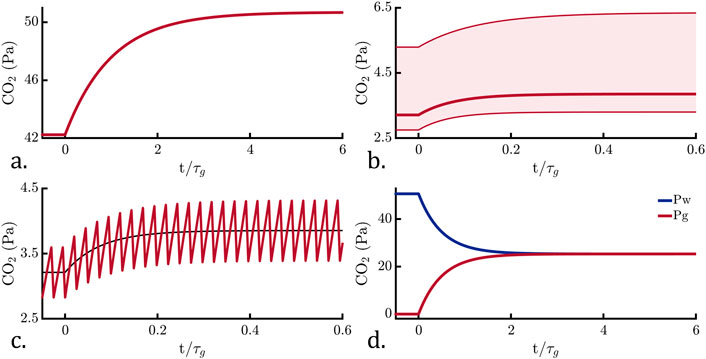
Figure 2. Computed step responses for the four modes, with the red lines indicating the gas-side CO₂ partial pressure. The x-axes are scaled with respect to the characteristic passive equilibration time, ${\tau }_g$, and the y-axes limits have been scaled to best display the data. (a) Passive equilibration. (b) Active equilibration. The bold line indicates the response under nominal dissolved gas conditions, whereas the shaded region indicates variation in response under different dissolved gas conditions (e.g., high or low oxygen). The limits of the shaded region correspond to the maximum and minimum variation in the other dissolved gases. (c) Hybrid equilibration. The black line indicates the active equilibration response, shown for comparison and to facilitate visualization of the step response curvature. When interpreted on a cycle-average basis (Section 5.3.2), the data follow the active equilibration response at a lower data rate. (d) Exchange equilibration. The blue line indicates the water-side pCO₂.

7 Optimization and design rules

7.1 Passive

Since the differential equation describing passive equilibration and its steady state and step response solutions were simple, the design insights are also simple. The only adjustable parameter is the instrument’s characteristic time response. The data will remain easy to interpret regardless of changes to ${\tau }_g$, because $P_w=P_g$ at steady state. The characteristic time is proportional to the gas-side volume and inversely proportional to the mass transport coefficient, membrane active area, and gas temperature. Therefore the time response may be improved by decreasing the internal gas volume, improving the mass transport characteristics of the membrane inlet, and increasing the active area. The mass transport characteristics may be improved by increasing flow rate to reduce the water-side stagnant boundary layer thickness, decreasing the thickness of the membrane, and increasing the permeability of the membrane to the target gas. While increasing the gas temperature would theoretically improve the time response, doing so would be impractical, as heating the gas volume may perturb the partial pressures of gases on the water-side of the membrane. The extent to which improving water flow characteristics (e.g., flow rate, geometry) will improve the time response depends on the gas.

Improving flow conditions has diminishing returns, and eventually the membrane inlet’s mass transport properties will be dictated solely by the membrane itself, and increasing the flow rate further will not improve the time response. Supplementary Section S4 explores the impact of the boundary layer on passive time response for different gases. Of the gases considered, CO₂ is less impacted by the boundary layer, and will reach membrane-limited mass transport at lower flow rates than other gases. An instrument’s time response in air and water should match if the flow rate is high enough to meet this condition; experimental verification may be helpful to confirm.

7.2 Active

The main advantage of active equilibration is that the time response can be significantly improved by reducing the vacuum level inside (i.e., setting $P_{\mathit{tot}}$). Figure 3 shows the characteristic time response versus vacuum level. The time response improves nonlinearly with decreasing $P_{\mathit{tot}}$. The trade-off of increased speed, however, is decreased steady state value. From Equation 22, the steady state value decreases by the same factor as increases in speed. In other words, an instrument with one-10th the time response also has one-10th the steady state gas level. Active equilibration requires much more sensitive gas-side instrumentation.

Figure 3

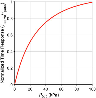
Figure 3. Characteristic times corresponding to computed active step responses for CO₂ under different operating pressures in the internal gas volume $(P_{\mathit{tot}})$. The active equilibration characteristic time was normalized by the passive equilibration time. As the total pressure drops, the relative reduction in time response improves. The range used goes up to 100 kPa to show that in the limiting case active and passive equilibration match, however there is little speed benefit to operating at these higher pressures.

Active equilibration has a second trade-off: cross-sensitivity, which occurs for all gases. Figure 4 shows the response of an active equilibration instrument operating at 2 kPa with the same variation in dissolved gas conditions as shown in Figure 2, again with the results under nominal gas conditions (bold lines), the variation due to other gases (shaded areas), and limits at the extremes (thin lines). For low concentration gases, like carbon dioxide and methane, the relationship between $P_{w,i}$ and $P_{g,i}$ is approximately linear. The linear response is because the total variation in these gases is not large enough to significantly impact the total gas flux into the instrument. The plots of oxygen and water vapor show a nonlinear relationship between $P_{w,i}$ and $P_{g,i}$ because their variation does significantly impact the total gas flux. If calibrations were conducted under nominal dissolved gas conditions, and the instrument were used in different conditions (e.g., during a depth profile from the surface through an oxygen minimum zone), significant errors in data interpretation would occur. It is not intuitive to expect cross-sensitivity from an instrument operation mode, especially if the gas-side instrumentation is highly selective to the target gas [e.g., a laser spectrometer Hodgkinson and Tatam (2012)]. Therefore, if cross-sensitivity was not checked in the laboratory, the resulting errors in field data may be especially difficult to detect and understand.

Figure 4

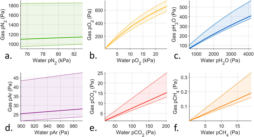
Figure 4. Computed instrument responses for different dissolved gas conditions under active equilibration. The bold lines indicate the response under nominal dissolved gas conditions. The thin lines indicate the response under extreme low and high dissolved gas conditions. The shaded areas show the variation within these limits. The instrument response would fall within the shaded area under any variation combination of all dissolved gases. Note the ranges on the axes. Variation relevant to oceanographic applications were used for all gases, as in Supplementary Table S3. Subfigures (a–f) display the computed results for nitrogen (pN₂), oxygen (pO₂), water (pH₂O), argon (pAr), carbon dioxide (pCO₂), and methane (pCH₄) .

The introduction of cross-sensitivity due to this active equilibration method is important to note, as it may not be an intuitive result. The effect of membrane selectivity on dissolved gas instrumentation has been noted in the oceanographic literature. Grilli et al. (2018) presented the design of a deep-sea laser spectrometer and included equations to relate its measurements to the external dissolved methane concentration. The instrument by Grilli et al. (2018) uses a methane-free sweep gas to extract dissolved methane from seawater via a deep-sea membrane inlet. Sweep gas equilibration is not covered here, but should work similarly to active equilibration because the flux of the target gas across the membrane is maximized but the total flow is mixed. Grilli et al. (2018) presented equations to convert measurements of methane and water vapor made by the laser spectrometer to dissolved methane concentrations that included oxygen, nitrogen and water vapor. The authors did conduct cross-sensitivity experiments for temperature and include results in the supplementary information, but did not mention any dissolved gas cross-sensitivity testing Grilli et al. (2018). Since oxygen, nitrogen, and water vapor appear in the conversion equations, variation in these gases might impact measurements, especially oxygen and nitrogen since they were not measured internally.

7.3 Hybrid

On average, hybrid equilibration tracks active equilibration, therefore conclusions from optimization of active equilibration can be used to help guide the design. As the average operational pressure decreases, the time response and the average steady state value decrease. The primary advantage of hybrid equilibration over active equilibration is that hybrid equilibration does not exhibit cross-sensitivity, so this need not be a consideration during optimization.

Hybrid equilibration’s main trade-off is its oscillatory nature, which complicates interpreting instrument data. Each ‘cycle’ of hybrid equilibration is fit to a line, and the resulting slope and intercept interpreted according to Equation 29. Since each cycle only returns one measurement, the data rate from the instrument is significantly reduced. This limits the bandwidth of the measurement (via the Nyquist theorem), and effectively constrains the timescale of the measurements.

To optimize a hybrid equilibration instrument design, it is critical to select an optimal dwell time. There must be enough time allotted to arrive at an adequate estimate for the slope and intercept, but longer dwell times reduce the overall bandwidth. Additionally, shorter dwell times will require more frequent vacuum operation, which reduces the amount of time the instrument is collecting useful data (only during equilibration phase). This trade-off depends on the specific noise properties of the gas-side instrumentation, and may require fine-tuning after the final instrument is built.

7.4 Exchange

The steady state and time response characteristics of exchange equilibration depend on the characteristic timescales of both the water-side and gas-side of the membrane inlet. As a result, there are now two variables to adjust to achieve the desired instrument performance. Figure 5 shows the step response of exchange equilibration under three different characteristic time conditions. In the plot ${\tau }_g$, is held constant and ${\tau }_w$, is varied. As ${\tau }_w$ decreases, the system responds faster, but the equilibrium value, $P_{\infty }$ decreases. As with active and hybrid equilibration, the instrument response time can be improved at the expense of lower steady state values.

Figure 5

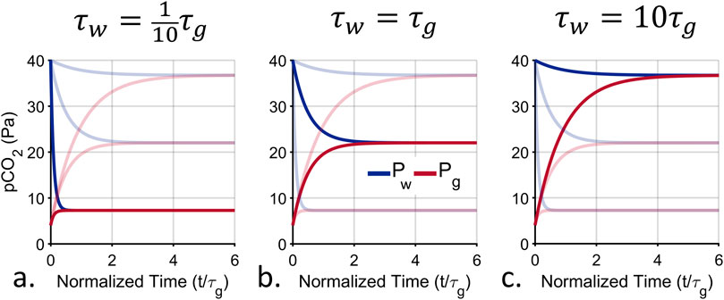
Figure 5. Computed exchange step response under different design conditions. There is a trade-off between speed and the magnitude of the final signal, dictated by the ratio of the water-side characteristic time, ${\tau }_w$, to the gas-side characteristic time, ${\tau }_g$. The red and blue traces indicate the partial pressure of CO₂ in the gas volume and water volume respectively. The faded lines show the other two conditions to facilitate comparison. For all, ${\tau }_g$ is held constant and ${\tau }_w$ is varied. (a) When ${\tau }_w<{\tau }_g$, the system response is fastest at the expense of the lowest equilibrium value. (b) When ${\tau }_w={\tau }_g$, the system response speed and equilibrium value fall between the conditions shown in the left and right plots. (c) When ${\tau }_w>{\tau }_g$, the response is slowest but has the highest equilibrium value. The response is almost the same as passive equilibration.

8 Discussion

Here, we derived analytical models for passive, active, hybrid and exchange equilibration to support the development of membrane-based dissolved gas instrumentation. The four operation modes were assessed for their steady state response and step response, and design rules and areas for optimization were identified.

Passive equilibration is straightforward: the differential equations are tractable, the steady state response is easy to interpret, there is no cross-sensitivity, and specific knowledge of membrane equilibration dynamics is not required to interpret results. The instrument design can be optimized for time response primarily by minimizing the gas volume, the membrane thickness and the water-side stagnant boundary layer and by maximizing the membrane area and the membrane permeability to the target gas. Passive equilibration is the slowest of all the techniques, and may not be useful if ${\tau }_g$ cannot be reduced enough in design optimization.

Active equilibration, by comparison is complicated: the differential equations are nonlinear and coupled, the steady state response requires detailed knowledge of membrane properties and dissolved gas conditions to interpret, and it is cross-sensitive. Active equilibration is much faster than passive equilibration, and would be more suitable when an instrument requires as fast a response as possible. The operating pressure for active equilibration is a key parameter for optimization, as it determines the time response of the instrument. Active equilibration requires more sensitive gas-side instrumentation, and noise present in the measurements will be amplified when computing $P_w$. The cross-sensitivity and required knowledge about the membrane dynamics will also introduce errors. Cross-sensitivity can be avoided by adding a mass flow meter.

Hybrid equilibration merges passive and active equilibration by alternating between the two. The dynamics during the equilibration phase of hybrid equilibration follow the straightforward passive equations. Hybrid equilibration matches the speed of active equilibration, and is not cross-sensitive. To interpret hybrid equilibration data, knowledge of the membrane properties for the gas of interest is required. Like active equilibration, the required dynamic range for the gas-side instrumentation is reduced. The main drawback of hybrid equilibration is the added complexity of interpreting the oscillatory data.

Exchange equilibration behaves like a discrete form of passive equilibration. While the equations that describe it are coupled, they are straightforward to solve analytically. Exchange equilibration can be optimized by reducing the water-side dissolved gas inventory, at the cost of reduced equilibrium gas pressure. To interpret the equilibrium value, knowledge of either the characteristic times or the inventories (i.e., volumes, solubility, temperatures, etc.) are required. There is no cross-sensitivity. Exchange equilibration performance can be improved using a vacuum or scrubbing the target gas. Exchange equilibation has higher mechanical complexity, as it generally requires active mixing and isolation valves.

Overall, we conclude that passive equilibration should be used if the design can be optimized to be fast enough for the intended application. Passive equilibration is the most straightforward to interpret, least complex, and does not require exact knowledge of the mass transport characteristics of the membrane in the system as implemented. If this is not possible, then time response correction, hybrid equilibration or active equilibration with mass flow monitoring are recommended for increasing response time. All do not incur cross-sensitivity as part of the cost of faster response. However, all amplify noise and may require much more sensitive gas-side instrumentation operating under vacuum. Exchange equilibration is more discrete in nature than the other methods, and should be chosen only for applications requiring this, such as a total dissolved inorganic carbon measurement, which requires in situ dosing of acid in a precise ratio to the sample.

We used a purely theoretical approach to derive the equations describing the dynamics of the equilibration methods, which represents a key limitation of this study. In the future, empirical evaluation of real dissolved gas instrumentation would be important to validate the results, particularly experiments to validate the design rules and cross-sensitivity observations. In addition, several key assumptions (Supplementary Section S2) were made in order to derive the analytical models in this study. These should be carefully assessed for specific designs, as these assumptions may not be valid for all instrument geometries.

Data availability statement

The original contributions presented in the study are included in the article/and in the Supplementary Material, further inquiries can be directed to the corresponding author.

Author contributions

BC: Conceptualization, Formal Analysis, Investigation, Methodology, Writing – original draft, Writing – review and editing. AM: Conceptualization, Funding acquisition, Project administration, Resources, Supervision, Writing – review and editing.

Funding

The author(s) declare that financial support was received for the research and/or publication of this article. Funding for this project was provided by the National Science Foundation under OCE-1454067.

Conflict of interest

The authors declare that the research was conducted in the absence of any commercial or financial relationships that could be construed as a potential conflict of interest.

Generative AI statement

The author(s) declare that no Generative AI was used in the creation of this manuscript.

Publisher’s note

All claims expressed in this article are solely those of the authors and do not necessarily represent those of their affiliated organizations, or those of the publisher, the editors and the reviewers. Any product that may be evaluated in this article, or claim that may be made by its manufacturer, is not guaranteed or endorsed by the publisher.

Supplementary material

The Supplementary Material for this article can be found online at: https://www.frontiersin.org/articles/10.3389/frmst.2025.1488800/full#supplementary-material

References

Baker, R. W. (2004). Membrane technology and applications. 2 edn. John Wiley and Sons, Ltd. doi:10.1002/0470020393

CrossRef Full Text | Google Scholar

Bass, A. M., Bird, M. I., Morrison, M. J., and Gordon, J. (2012). CADICA: Continuous automated dissolved inorganic carbon analyzer with application to aquatic carbon cycle science. Limnol. Oceanogr. Methods 10, 10–19. doi:10.4319/lom.2012.10.10

CrossRef Full Text | Google Scholar

Bell, R. J., Short, R. T., van Amerom, F. H. W., and Byrne, R. H. (2007). Calibration of an in situ membrane inlet mass spectrometer for measurements of dissolved gases and volatile organics in seawater. Environ. Sci. and Technol. 41, 8123–8128. doi:10.1021/es070905d

PubMed Abstract | CrossRef Full Text | Google Scholar

Chua, E. J., Savidge, W., Short, R. T., Cardenas-Valencia, A. M., and Fulweiler, R. W. (2016). A review of the emerging field of underwater mass spectrometry. Front. Mar. Sci. 3. doi:10.3389/fmars.2016.00209

CrossRef Full Text | Google Scholar

Cussler, E. L. (2009). Diffusion: Mass transfer in fluid systems. 3 edn. Cambridge University Press.

Google Scholar

Doney, S. C., Fabry, V. J., Feely, R. A., and Kleypas, J. A. (2009). Ocean acidification: the other CO₂ problem. Annu. Rev. Mar. Sci. 1, 169–192. doi:10.1146/annurev.marine.010908.163834

PubMed Abstract | CrossRef Full Text | Google Scholar

Fietzek, P., Fiedler, B., Steinhoff, T., and Körtzinger, A. (2014). In situ quality assessment of a novel underwater pCO₂ sensor based on membrane equilibration and NDIR spectrometry. J. Atmos. Ocean. Technol. 31, 181–196. doi:10.1175/JTECH-D-13-00083.1

CrossRef Full Text | Google Scholar

Grilli, R., Triest, J., Chappellaz, J., Calzas, M., Desbois, T., Jansson, P., et al. (2018). Sub-Ocean: subsea dissolved methane measurements using an embedded laser spectrometer technology. Environ. Sci. and Technol. 52, 10543–10551. doi:10.1021/acs.est.7b06171

PubMed Abstract | CrossRef Full Text | Google Scholar

Halpern, B. S., Frazier, M., Afflerbach, J., Lowndes, J. S., Micheli, F., O’Hara, C., et al. (2019). Recent pace of change in human impact on the world’s ocean. Sci. Rep. 9, 11609. doi:10.1038/s41598-019-47201-9

PubMed Abstract | CrossRef Full Text | Google Scholar

Hodgkinson, J., and Tatam, R. P. (2012). Optical gas sensing: a review. Meas. Sci. Technol. 24, 012004. doi:10.1088/0957-0233/24/1/012004

CrossRef Full Text | Google Scholar

Hopkins, F. E., Suntharalingam, P., Gehlen, M., Andrews, O., Archer, S. D., Bopp, L., et al. (2020). The impacts of ocean acidification on marine trace gases and the implications for atmospheric chemistry and climate. Proc. R. Soc. A Math. Phys. Eng. Sci. 476, 20190769. doi:10.1098/rspa.2019.0769

PubMed Abstract | CrossRef Full Text | Google Scholar

Levin, L. A. (2018). Manifestation, drivers, and emergence of open ocean deoxygenation. Annu. Rev. Mar. Sci. 10, 229–260. doi:10.1146/annurev-marine-121916-063359

PubMed Abstract | CrossRef Full Text | Google Scholar

McNeil, C., D’Asaro, E., Johnson, B., and Horn, M. (2006). A gas tension device with response times of minutes. J. Atmos. Ocean. Technol. 23, 1539–1558. doi:10.1175/JTECH1974.1

CrossRef Full Text | Google Scholar

Michel, A. P., Wankel, S. D., Kapit, J., Sandwith, Z., and Girguis, P. R. (2018). In situ carbon isotopic exploration of an active submarine volcano. Deep Sea Res. Part II Top. Stud. Oceanogr. 150, 57–66. doi:10.1016/j.dsr2.2017.10.004

CrossRef Full Text | Google Scholar

Nagy, E. (2019). Basic equations of the mass transport through a membrane layer. Elsevier. doi:10.1016/C2011-0-04271-0

CrossRef Full Text | Google Scholar

Reay, D. S., Smith, P., Christensen, T. R., James, R. H., and Clark, H. (2018). Methane and global environmental change. Annu. Rev. Environ. Resour. 43, 165–192. doi:10.1146/annurev-environ-102017-030154

CrossRef Full Text | Google Scholar

Reed, A., McNeil, C., D’Asaro, E., Altabet, M., Bourbonnais, A., and Johnson, B. (2018). A gas tension device for the mesopelagic zone. Deep Sea Res. Part I Oceanogr. Res. Pap. 139, 68–78. doi:10.1016/j.dsr.2018.07.007

CrossRef Full Text | Google Scholar

Santos, I. R., Maher, D. T., and Eyre, B. D. (2012). Coupling automated radon and carbon dioxide measurements in coastal waters. Environ. Sci. and Technol. 46, 7685–7691. doi:10.1021/es301961b

PubMed Abstract | CrossRef Full Text | Google Scholar

Sarmiento, J. L., and Gruber, N. (2006). Ocean biogeochemical dynamics. Princeton University Press.

Google Scholar

Takahashi, T., Sutherland, S. C., Sweeney, C., Poisson, A., Metzl, N., Tilbrook, B., et al. (2002). Global sea–air CO₂ flux based on climatological surface ocean pCO₂, and seasonal biological and temperature effects. Deep Sea Res. Part II Top. Stud. Oceanogr. 49, 1601–1622. doi:10.1016/S0967-0645(02)00003-6

CrossRef Full Text | Google Scholar

Talley, L., Feely, R., Sloyan, B., Wanninkhof, R., Baringer, M., Bullister, J., et al. (2016). Changes in ocean heat, carbon content, and ventilation: A review of the first decade of GO-SHIP global repeat hydrography. Annu. Rev. Mar. Sci. 8, 185–215. doi:10.1146/annurev-marine-052915-100829

PubMed Abstract | CrossRef Full Text | Google Scholar

Tortell, P. D. (2005). Dissolved gas measurements in oceanic waters made by membrane inlet mass spectrometry. Limnol. Oceanogr. Methods 3, 24–37. doi:10.4319/lom.2005.3.24

CrossRef Full Text | Google Scholar

Wankel, S. D., Germanovich, L. N., Lilley, M. D., Genc, G., DiPerna, C. J., Bradley, A. S., et al. (2011). Influence of subsurface biosphere on geochemical fluxes from diffuse hydrothermal fluids. Nat. Geosci. 4, 461–468. doi:10.1038/ngeo1183

CrossRef Full Text | Google Scholar

Wankel, S. D., Huang, Y.-w., Gupta, M., Provencal, R., Leen, J. B., Fahrland, A., et al. (2013). Characterizing the distribution of methane sources and cycling in the deep sea via in situ stable isotope analysis. Environ. Sci. and Technol. 47, 1478–1486. doi:10.1021/es303661w

PubMed Abstract | CrossRef Full Text | Google Scholar

Wankel, S. D., Joye, S. B., Samarkin, V. A., Shah, S. R., Friederich, G., Melas-Kyriazi, J., et al. (2010). New constraints on methane fluxes and rates of anaerobic methane oxidation in a Gulf of Mexico brine pool via in situ mass spectrometry. Deep Sea Res. Part II Top. Stud. Oceanogr. 57, 2022–2029. doi:10.1016/j.dsr2.2010.05.009

CrossRef Full Text | Google Scholar

Wanninkhof, R., Park, G.-H., Takahashi, T., Sweeney, C., Feely, R., Nojiri, Y., et al. (2013). Global ocean carbon uptake: magnitude, variability and trends. Biogeosciences 10, 1983–2000. doi:10.5194/bg-10-1983-2013

CrossRef Full Text | Google Scholar

Webb, J. R., Maher, D. T., and Santos, I. R. (2016). Automated, in situ measurements of dissolved CO₂, CH₄, and δ¹³C values using cavity enhanced laser absorption spectrometry: Comparing response times of air-water equilibrators. Limnol. Oceanogr. Methods 14, 323–337. doi:10.1002/lom3.10092

CrossRef Full Text | Google Scholar

Wijmans, J., and Baker, R. (1995). The solution-diffusion model: a review. J. Membr. Sci. 107, 1–21. doi:10.1016/0376-7388(95)00102-I

CrossRef Full Text | Google Scholar

Wijmans, J. G., Athayde, A. L., Daniels, R., Ly, J. H., Kamaruddin, H. D., and Pinnau, I. (1996). The role of boundary layers in the removal of volatile organic compounds from water by pervaporation. J. Membr. Sci., 109. doi:10.1016/0376-7388(95)00194-8

CrossRef Full Text | Google Scholar

Wijmans, J. G., and Baker, R. W. (2006). “The solution–diffusion model: A unified approach to membrane permeation,”. John Wiley and Sons, Ltd, 159–189. chap. 5. doi:10.1002/047002903X.ch5

CrossRef Full Text | Google Scholar

Yoon, T. K., Jin, H., Oh, N.-H., and Park, J.-H. (2016). Technical note: Assessing gas equilibration systems for continuous pCO₂ measurements in inland waters. Biogeosciences 13, 3915–3930. doi:10.5194/bg-13-3915-2016

CrossRef Full Text | Google Scholar