Real-time Hand Motion Reconstruction System for Trans-Humeral Amputees Using EEG and EMG

Introduction

Motion reconstruction refers to the problem of predicting an extremity’s position using only biosignals for reconstructing, without using any cameras or tracking devices. The main application for this kind of system is the control of a prosthetic device. Nevertheless, applications, such as videogames or robot control, are also possible.

Depending on which part of the trajectory of the extremity is reconstructed, there are different challenges. A distal part of the extremities, such as a hand or foot, is easier to reconstruct than a proximally amputated part, such as an arm or leg. This is mainly because most of the muscles related to foot and hand movements are still active in the leg and arm; thus, it is possible to predict the intention with electromyography (EMG) signals detected from those muscles. Foot prostheses have achieved high accuracy (Au et al., 2008) due to the low number of Degrees of Freedom (DoF) and well-known dynamics. Although the hand has a higher number of DoF, its reconstruction also achieved high accuracy. In the case of the hand, there are different challenges, such as reconstruction of each one of the fingers (Tenore et al., 2007) or cheaper development of the prosthetic device (Zuniga et al., 2015). Above-knee prostheses have fewer DoF than hand prostheses, but in this case, the number of the remaining motion-related muscles is lower. Yet, since the motion dynamics of the leg are well known, it is possible to create reliable above-knee prostheses (Seliktar and Kenedi, 1976; Jung-Hoon and Jun-Ho, 2001). Finally, shoulder prostheses (those used for trans-humeral amputees) are the most complex ones. The number of DoF is larger than for any other prostheses (in theory, the system should be able to reconstruct the motion of the shoulder, elbow, wrist, and fingers); on the other hand, the number of remaining motion-related muscles is very low, and the dynamics of the arm are complex and difficult to predict. The final objective is to build a system in which the prosthetic device moves as a real arm would.

Due to the lack of remaining motion-related muscles, the information from the EMG is not enough to completely implement the control of shoulder prosthesis. Thus, brain computer interfaces (BCI) are used to improve the reconstruction accuracy. The most precise control is usually achieved by using invasive technologies (Gilja et al., 2012; Hochberg et al., 2012); such technologies are also used for sensory restoration (Tabot et al., 2013). However, these approaches require brain surgery, which could cause brain damage, and need further safety inspection. Consequently, these kinds of approaches are only used experimentally with animals or in extreme cases of paralysis. Thus, a method using non-invasive technologies should be developed in order to promote the use of shoulder prostheses.

Full arm motion reconstruction has been addressed by a few studies. Generally, the problem is simplified when using non-invasive technologies by, for example, reducing the number of DoF that are reconstructed (Lv et al., 2010; Robinson et al., 2013; Kim et al., 2014). In those cases, only electroencephalography (EEG) was used. This approach is the most general one; for any amputee, we can assume that the EEG is available, while some muscles may be present or not depending on the subject. The main problem of this approach is that the obtained correlation values (CVs) between the real and the reconstructed trajectory are too low, up to 0.6 in the best-case scenario. Other studies, such as Kiguchi and Hayashi (2013), using a combination of EEG and EMG obtained almost perfect scores. This approach, nevertheless, places the EMG along the arm. Thus, it may be applicable to videogames or robot control, but not to prosthesis control.

In this study, we present an approach to solve the arm motion reconstruction problem, taking into consideration the following aspects. First, our main goal is to use this approach for trans-humeral amputees in real life. Therefore, the system should be able to work in real time and should not use EMG located beyond the humerus. To be certain that our system is usable by most trans-humeral amputees, the only muscle located in the arm that we used was the deltoidus. This muscle is present, by definition, in every trans-humeral amputee, and it carries a lot of motion-related information. The second characteristic of our system is that it only predicted the position of the hand in three dimensions (x, y, and z). This means that it did not predict the position of the elbow or its rotation. It neither predicted the angle of the wrist nor the position of the fingers. We reconstruct only for the hand’s position since the elbow position is not as important for conducting everyday living activities, such as pointing or grasping. In the case of the wrist and fingers, we do not reconstruct them since it is too difficult to do for the moment. Finally, we use both EEG and EMG, and make clear their contribution to the reconstruction. Even if these systems are intrinsically related (Halliday et al., 1998; Grosse, 2002; Hashimoto et al., 2010), different information can be extrapolated from them.

Previous Work

We divided our study into three stages: predictor proposal, system optimization, and feature analysis. In the first one, we proposed four different architectures based on artificial neural networks (ANNs) as predictors for the system (Fernandez-Vargas et al., 2015). Those architectures were combined with different inputs to create eight different approaches. This paper presents the results obtained in this first stage and further research efforts based on the results.

With the results obtained from the first stage, we selected the two best ones for the next stage based on their final CVs. In the second stage, we optimized the input and configuration of the selected approaches for removing redundant information. We also added the estimated previous positions as the input to the system to see the effect (Fernandez-Vargas et al., 2016).

In the last stage, we analyzed the importance of the different signal sources, the amount of information that they provide, and the topography of the relation between the motion and the brain activation.

The paper is organized as follows: in the Section “Materials and Methods,” the experiment task, data processing, classification and optimization procedures, and statistical methods are described; in the Section “Results,” analyses and comparison of different approaches are presented; furthermore, the effects of the optimization process and the information analyses are shown; finally, in the Section “Discussion,” we discuss the interpretation of the data, the limitations, and future studies.

Materials and Methods

Text from Section “System” and “Predictor Proposal” has been adapted from Fernandez-Vargas et al. (2015), including Figures 1 and 3.

FIGURE 1

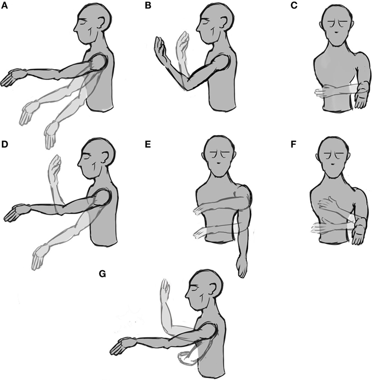
Figure 1. Representation of the seven phases with movement. (A–C) simple movements, i.e., the motion occurs only on one DoF, (D–F) combined movements, i.e., the movement occurs on two DoFs, and (G) the hand’s free movement.

System

Experiment Subjects

A sample of N = 16 healthy young adults participated in the experiment. Our sample consisted of eight females and eight males. Permission from the ethics committee of the Graduate School of Engineering, Chiba University was obtained. All subjects participated voluntarily, giving informed consent without receiving any incentives. Participants were informed that they could stop the experiment at any time.

Task

The experiment was designed considering the future use of the system for controlling a wearable prosthetic device; therefore, there are some a priori restrictions. First, the number of DoF is limited. We chose three movements that allow placing the hand in almost any position with a wearable prosthesis. The three DoFs are two for the shoulder [up and down (Figure 1A) and rotation (Figure 1C)] and one for the elbow [flexion and extension (Figure 1B)]. With these three movements, the subject can reach any point in front of him/her. The second limitation arising from using a wearable prosthetic device is that the speed that the machine can reach is limited, especially if we take into consideration the system stability. Therefore, subjects were asked to move the arm slowly (not faster than around 60°/s). At this speed, it is possible to grasp an object and pass it to another person in less than 5 s.

The experiment was divided into eight phases, and each is separated from the successive ones by a resting time of 20 s in which we explained to the subject the next phase. The first phase was a 60-s baseline in which the subject was asked to stay still and try to avoid blinking or ocular movements in order to avoid EEG artifacts. During the following phases, the subject was instructed to move the arm according to a specific set of movements. From phase two to four (the first row in Figure 1), the subject was asked to perform three simple movements for 20 s. In this case, by “simple” we mean that the movement takes place only across one DoF. From phase five to seven (the second row in Figure 1), the subject was asked to perform a combined movement for another 20 s, which meant moving the arm along two DoFs. Finally, for the last phase, the subject was instructed to move the arm freely across three DoFs for 60 s (Figure 1G). This process was performed only once per subject. The whole experiment (including the setup) took less than 40 min. All data were saved for a posteriori off-line analysis.

Data Acquisition

Three synchronized systems were used for acquiring the data:

• EEG (input): an EEG cap (BioSemi ActiveTwo) recording device with 16 active electrodes. The electrodes were positioned at Fz, F2, F4, F6, F8, FCz, FC2, FC4, FC6, Cz, C2, C4, Pz, P2, Oz, and O2, according to the international 10–20 system, as shown in Figure 2A. The locations of the electrodes were chosen to primarily cover the motor cortex, parietal, and occipital area as suggested in Waldert et al. (2008), Bradberry et al. (2010), Lv et al. (2010), and Schoffelen et al. (2011). Since the task of the experiment consisted of moving the left arm, the electrodes were located in the center and right hemisphere of the scalp.

FIGURE 2

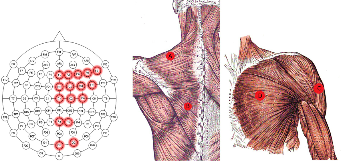
Figure 2. Electrode location diagram. Those EEG electrodes used for the recordings are highlighted in red in the left image. The approximated location of the EMG electrodes for the trapezius (A,B) is presented in the middle. The approximated location of the EMG electrode for the deltoideus (C), and pectoralis major (D) are presented in the right image. The middle and right figure are adapted from Gray and Carter (1858).

• EMG (input): four surface EMG electrodes connected to an NI USB-6210 amplifier. Two of the EMG’s electrodes were placed in the left trapezius (location A and B in Figure 2), one on the left deltoideus (location C in Figure 2), and one on the left pectoralis major (location D in Figure 2) (see Figure 2B). These locations were chosen to acquire the information relative to the arm’s movement without placing them on the arm, following Horiuchi et al. (2009).

• Motion Tracking (output): OptiTrack’s arena 1.7 software with nine Flex 3 cameras was used. This system tracks the physical position (x, y, and z) of three rigid body markers attached to the subject on the left shoulder, left elbow, and left hand, respectively. The relative coordinate values corresponding to the hand using the shoulder as the origin were the predicted values using the EEG and EMG signals.

The three acquisition systems recorded signals at 1024 Hz.

Preprocessing

Both EEG and EMG signals were divided into windows of 1 s with 87.5% overlap. This means that there were eight different windows per second. For the EEG, a detrending window and a Hamming window were applied. After this, a process, similar to the one used in Lv et al. (2010), was performed to extract the EEG’s features. For each EEG window, the corresponding FFT was calculated. The result of the FFT was divided into 10 bands of 4 Hz (from 1 to 40 Hz with a resolution of 1 Hz), and the total power for those bands was computed. In addition, the mean value of the 60-s baseline was calculated for each band. Using the baseline, the signal to noise ratio (SNR) of those same bands was calculated as follows:

${\text{SNR}}_i=\frac{P_i}{P_{iBaseline}},$

where P_i is the power of the i-th band, and $P_{iBaseline}$ is the mean power for the same band during the baseline. Altogether, 20 values were calculated as the final output for each EEG channel.

For describing the EMG, 13 values were calculated for each channel and window. These features were selected from Zardoshti-Kermani et al. (1995), Fukuda et al. (2003), and Phinyomark et al. (2010): integrated EMG (IEMG), mean absolute value (MAV), modified mean absolute value 1 (MAV1), modified mean absolute value 2 (MAV2), mean absolute value slope (MAVS), simple square integral (SSI), variance (VAR), root mean square (RMS), waveform length (WL), zero crossing (ZC), slope sign change (SSC), Wilson amplitude (WAMP), and square sum of EMG (SSM). For further details of these features, please refer to Fernandez-Vargas et al. (2015).

Only time domain features were computed, because frequency domain features do not lead to clear improvement, although they are more computationally expensive (Phinyomark et al., 2010).

At the end of preprocessing, we obtained 372 features, 10 from each EEG channel’s FFT power bands (160), 10 from each EEG channel’s SNR power bands (160), and 13 from each EMG channel (52). We calculated the mean value and the SD for each of those features and then normalized each of them. This high dimensional feature vector is used as the input for the predictors.

Even though the preprocessing was performed offline, our tests confirmed that it can be done online. As mentioned in Section “Information Importance,” we used a 1-s window at 1024 Hz with an overlapping of 87.5%, which means that we performed the complete preprocessing eight times per second. The complexity of the process depends on the length (N) of the window. Regarding the EEG features, the operation performed was an FFT, which has a complexity O(NlogN). For calculating the EMG features, all the operations were linear, and thus, had a complexity of O(N). In conclusion, the complexity of the preprocessing is O(NlogN).

Regarding the output, we calculated the three position coordinates (x, y, and z) of the hand. For each input, we had 1024 samples of each coordinate. Since we wanted to calculate only one value, we apply a Hamming window to those values and compute the mean. Hence, each output is an array with three elements, calculated from an input array of length 372.

Many BCI studies use other preprocessing procedures, such as spatial filters (Liao et al., 2007) or independent component analysis (Lv et al., 2010). However, these procedures typically require that the output is a discrete value. Consequently, it is impossible to use them for continuous position reconstruction (Blankertz et al., 2008).

Predictor Proposal

Predictor Design

For solving the reconstruction problem, it is important to choose the right predictor. Many predictors have binary output, which enables differentiations between two classes. Other predictors can handle N classes. For this problem, we need a predictor that can handle continuous output values for predicting the hand’s position. We chose ANNs.

We employed the scaled conjugate gradient algorithm for training all ANNs (Møller, 1993), using the Neural Network Toolbox from Matlab^®. As the transfer function for the hidden layer, we used the hyperbolic tangent sigmoid and a linear transfer function for the output layer. Since there is no established method to preselect the number of neurons in the hidden layers, we decided to use two-thirds of the size of the input plus output. We found that the number of neurons in the hidden neuron is essential for getting optimal results. Nevertheless, since the number of training–validation iterations that have to be performed was too high, we could not add more analysis to search for an optimal number of hidden neurons in each network. This process was performed afterward for two of the predictors (see Optimization).

We implemented four different predictors, as described below (Figure 3).

FIGURE 3

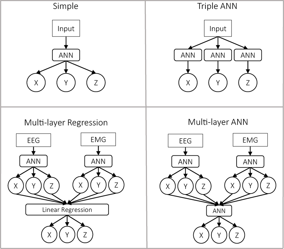
Figure 3. Representation of the four predictor approaches. In the first row are presented the approaches with a single layer. In those cases, the input can be either only EEG, only EMG, or the concatenation of EEG and EMG as a single vector. In the case of the multilayer approaches, the data are always separated.

Classical Predictor (Simple Predictor)

As input, we used a single vector. The predictor itself was an ANN, which predicts the three outputs x, y, and z. This is the most simple and common approach in the literature to solve this problem.

Triple-ANN Predictor

As input, we used a single vector. Then, we used three different ANNs to predict each of the outputs independently. Theoretically, this predictor should be very similar to the previous one, with three times the number of neurons in the hidden layer.

Multilayer Regression Predictor

In the first layer, we had two ANNs similar to the one used in the classical approach. Nevertheless, in this case, the input was divided into EEG and EMG, so each ANN predicted the output based only on one of the inputs. At the second layer, we performed a linear regression for each dimension, using the outputs of both ANNs as inputs.

Multilayer ANN Predictor

Similar to the previous predictor, the data were divided into EEG and EMG. The difference was that for predicting the final output, we used a third ANN whose inputs were the outputs of the previous two ANNs. This second ANN was trained once the first two had finished their training.

In the case of the classical predictor and the triple-ANN predictor, we used three kinds of input data: the complete data (EEG + EMG), only EEG, and only EMG. As a result of these combinations, we had eight different approaches in total: complete data using the simple approach (CPS), complete data using the triple-ANN approach (CPT), only EEG using the simple approach (EES), only EEG using the triple-ANN approach (EET), only EMG using the simple approach (EMS), only EMG using the triple-ANN approach (EMT), separated data using the multilayer regression approach (SMR), and separated data using the multilayer ANN approach (SMA).

Evaluation

Every time we trained an ANN, the recorded data were randomly divided into training (70%), testing (15%), and validation (15%). The training was repeated 30 times for each analysis. This process was done for every subject. The input data for the ANN are the preprocessed values for each time window. Since there are ~180 s of valid recording (20 s for each of the six motions plus 60 s of free motion) and 87.5% of overlapping, there are ~1440 samples for each subject.

For calculating the final CV, we used the validation data and calculated the CV between the output of the predictor and the real trajectory for each dimension. Then, we took the median across the 30 repetitions of the training and the mean value of the three dimensions (x, y, and z) as the final CV.

Optimization

Dimensionality Reduction

After analyzing the results from the previous approaches, we optimized the ANN architectures of the two approaches, CPS and SMR, based on the results shown in Section “Results.” The optimization process was done after the first group of results, since part of the process was highly computationally expensive. Thus, it was not possible to apply it for every predictor approach. The optimization was divided into two steps. The first one was the feature selection. The second one was the optimization of the number of neurons in the ANNs.

For the feature selection, we calculated the correlation between each pair of features, separating EEG and EMG. We removed one of the features in those pairs with a correlation higher than 0.95. For the EEG, we removed the SNR values following this process, i.e., 50% of the EEG data we were using were redundant.

In the case of the EMG, we removed the features MAV, MAV1, VAR, RMS, and WL, i.e., 38% of the EMG data we were using were redundant.

For optimizing the number of neurons for the CPS, we repeated the evaluation process 30 times for each subject and configuration, varying the number of neurons from 5 to 400 in steps of 5 neurons (i.e., 80 different ANN configurations). We selected the ANN configuration with maximum mean correlation across all subjects as the optimal ANN configuration. In this case, the number of neurons was set to 145 neurons.

For the SMR, we followed a similar process. Nevertheless, SMR had two separated ANNs, the one that reconstructed the movement from the EEG and the one that used the EMG data. Finding the optimal number of neurons for each of them was not enough to obtain an optimal result, so we needed to test the combination of different ANN configurations. For the ANN in charge of the EEG, we tested from 20 to 250 neurons. For the ANN in charge of the EMG, we tested from 20 to 180 neurons. Thus, the number of possible ANN configurations that we tested was 1551. We selected the combination of the ANN configuration with the maximum mean correlation across all subjects as optimal. As a result, we determined that the optimal number of neurons for the ANN in charge of the EEG was 130, and the optimal number of neurons for the ANN in charge of the EMG was 45.

Temporal Information

After the optimization process, we added temporal information to seek the possibility of further improving the system. We conducted this process only for the CPS and SMR approaches, based on the results shown in Section “Results.”

For the previous approaches, the prediction at moment t was done by using only EEG and EMG data at the moment. They are defined as:

$\text{CPS}\left(t\right)=\text{ANN}\left(\text{EEG}\left(t\right)+\text{EMG}\left(t\right)\right),$

$\text{SMR}\left(t\right)=\text{LR}\left(\text{ANN}\left(\text{EEG}\left(t\right)\right)+\text{ANN}\left(\text{EMG}\left(t\right)\right)\right),$

where “+” stands for the concatenation of vectors, LR means the linear regression function, and ANN means an ANN function. For example, $\text{ANN}\left(\text{EEG}\left(t\right)+\text{EMG}\left(t\right)\right)$ corresponds to the output of the ANN that has as input, the concatenation of the data from the EEG at time = t and the data from the EMG at the same time t. We decided to create a new approach using the previously estimated points. We called these approaches temporal CPS_N (TCPS_N) and temporal SMR_N (TSMR_N). We defined them as follows:

${\text{TCPS}}_N\left(t\right)=\text{ANN}\left(\text{EEG}\left(t\right)+\text{EMG}\left(t\right)+{\displaystyle \sum _{i=1}^N}{\text{TCPS}}_N\left(t-i\right)\right),$

$\begin{array}{c}{\text{TSMR}}_N\left(t\right)=\text{LR}\left(\text{ANN(EEG(t)})+\text{ANN(EMG(t))+}{\displaystyle \sum _{i=1}^N{\text{TSMR}}_N(t-i)}\right),\end{array}$

where N is the number of time steps taken into consideration. Since we used a time window of 1 s with an 87.5% overlap, each time step corresponded to 0.125 s. Thus, N = 8 takes into consideration all the previously estimated positions from t − 1 s. The TCPS_N approach is also known as a non-linear autoregressive neural network with external input (NARX) (Leontaritis and Billings, 2007).

There are two important points to consider. First, TSMR₀ should be the same as SMR, since as in the former case, there would not be temporal information. However, we use the name SMR for the approach without optimization and TSMR₀ for the approach with optimization. The same reasoning can be applied to CPS and TCPS₀. Second, the temporal data in the TSMR approach were added in the linear regression layer, while the ANN layer was left unchanged. We tested these approaches by changing N from 0 to 8.

Finally, since we needed the previously estimated points to reconstruct the next point, the training method was slightly modified for the TCPS_N approaches. Instead of using random points, the data were divided into three consecutive blocks, maintaining the proportion 70, 15, and 15 for training, testing, and validation, respectively.

Information Importance

Four analyses were performed to calculate the importance of different dimensions of the system.

In the first analysis, we calculated the importance of different channels (both EEG and EMG). For this analysis, we used the TCPS₀ approach. After training the network and calculating the original CV, we replaced each channel with zeros (since the mean value of each channel is zero), one at a time. Using the new data as input for the predictor, we calculated the new CV. Subtracting the original CV from the new CV showed the contribution of that variable to the final output. We performed this process for each channel and normalized the result across all channels to obtain their relative importance. This was an empirical method that we called Zero Substitution. We compared these results with those obtained by the theoretical Goh measure described by Goh (1995).

The second analysis focused only on the EEG channels, to investigate the topology of their importance in the scalp. In this case, we compared two different descriptors. The first one was the result obtained in the previous analysis with the Zero Substitution method. In addition, we used the Source Power Comodulation (SPoC) method (Dähne et al., 2014) between the hand’s position and the raw data signal. SPoC returns a group of spatial filters based on the covariance between two signals. In this case, we used the raw EEG signals of the raw hand’s position. We used the normalized absolute values of the filter with the highest correlation between both signals. We computed both descriptors separately for each one of the three dimensions x, y, and z.

Using the Zero Substitution method, we also calculated the importance of each feature used during the optimization. In this case, instead of substituting each channel, we substituted each feature for all channels.

The last analysis aimed to compare the different systems (EEG, EMG, and temporal information). The TSMR_N approach with different configurations was used. For doing so, we extracted the regression coefficients obtained in the second layer to calculate the importance of each system. We also normalized the results in this case. Intuitively, if a system has a high regression coefficient, it means that the system is highly correlated with the output, while having a lower regression coefficient means a poor correlation.

Statistical Analysis

Predictor Proposal

Different statistical analyses were performed in order to decide which approach was better. For comparing the eight predictor approaches defined in subsection predictors (CPS, CPT, EES, EET, EMS, EMT, SMR, and SMA), we used a Kruskal–Wallis analysis (Kruskal and Wallis, 1952). We did not use a parametric test, such as ANOVA (Fisher, 1925), since the data do not fulfill the homoscedasticity and normal distribution pre-assumptions.

Furthermore, in order to calculate the corresponding p-value of every comparison of the Kruskal–Wallis analysis, we performed a post hoc analysis using the Fisher’s least significant difference procedure and calculated the size effect using Cohen’s Δ (Muller, 1989).

Using a priori statistical test power analysis with the program G*Power 3 (Faul et al., 2007) showed that the Pearson correlation significance test, using a sample size of 16 and with a significance level of α = 0.05, has a test power (1 − β) > 0.8, as suggested by Cohen (1988) when there is an effect size in the population with ρ ≥ 0.60. Thus, even if the employed sample size is relatively small, hypothesis testing of the Pearson correlation was possible at the level of assumed large effect sizes.

Optimization

To test whether there was any difference between the optimized approaches (TCPS₀ and TSMR₀) and the original approaches (CPS and SMR), two Student’s t-tests (Gosset, 1908) were executed. For deciding the best configuration for each predictor, we selected the one with the highest CV for each one. Then, we used a t-test to see if there was any difference between the two predictors. Finally, an ANOVA analysis was performed to check for differences between the TSMR_N approaches.

Results

Figures 5 and 6 have been adapted from Fernandez-Vargas et al. (2016). Still, all the calculations (including the ANN trainings) were done again using the same process for every analysis. New versions include more data and have been reshaped to make it clearer.

Predictor Comparison

The final CVs (calculated as explained in Section “Evaluation”) for the eight different approaches are presented in Table 1. The best approach is highlighted for each subject. The best approach for eight of them was CPS, for seven was SMR, and for one of them was SMA. None of the other approaches were the best for any subject.

TABLE 1

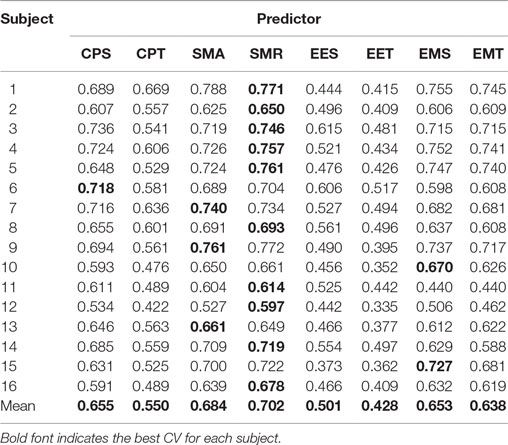
Table 1. Predictors result.

Table 2 shows the post hoc analysis. Approaches were compared two by two. For each approach, the difference of means, the p-value of Fisher’s least significant difference procedure, and Cohen’s Δ are presented. A positive mean difference means that the first approach is better, while a negative value indicates the second approach is better. The p-value column indicates the result of such a comparison. Finally, Cohen’s Δ column indicates the size effect of the difference.

TABLE 2

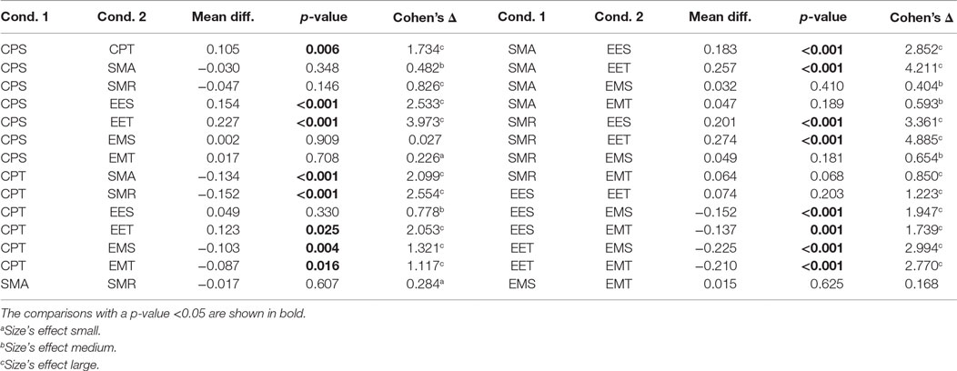
Table 2. Predictors post hoc results.

These results show that there are two groups of predictors. On the one hand, the group with the highest CV is the one including the EMG data. The second group is formed by EES and EET (i.e., those predictors that take into consideration only EEG). There is an exception that CPT has a lower CV than the rest of the predictors for their corresponding groups; this is most likely due to an over-fitting problem. There are no statistical differences within groups. All the possible pairs between those two groups have a large size effect. Graphical representation of Tables 1 and 2 can be seen in Figure 4.

FIGURE 4

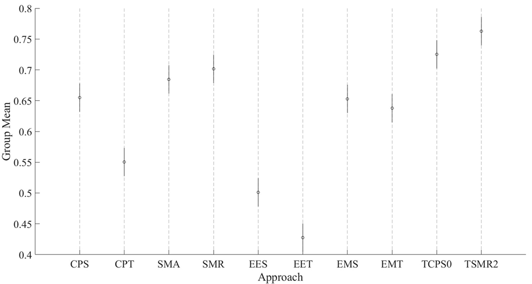
Figure 4. Comparison of the eight initial approaches plus the two best optimization results. Each line represents the 95% confident interval for each of them. The circle in the middle corresponds to the mean for that group. Overlapping intervals between two approaches means that they were not significantly different.

In order to see whether there was an increasing error with the speed, we calculated the correlation between the speed, calculated as the distance between two consecutive points, and the error for each dimension. We found no statistically significant correlation between the variables.

Optimization and Temporal Information

Table 3 presents the results for the optimization and temporal information. The TCPS₀ and TSMR₀ columns correspond to the optimization of CPS and SMR, respectively.

TABLE 3

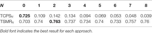
Table 3. Optimization and temporal information results.

• The mean difference between TCPS₀ and CPS is 0.07 (i.e., an increment of 11%). The p-value resulting from the t-test of this comparison was <0.001.

• The mean difference between TSMR₂ and SMR is 0.06 (i.e., an increment of 8%). The p-value resulting from the t-test of this comparison was <0.001.

• The difference between TSMR₂ and TCPS₀ is 0.03 (i.e., an increment of 5%). The p-value resulting from the t-test of this comparison was <0.001.

The best result achieved during the optimization was a CV of 0.855 for subject # 9 with the TSMR₄ approach.

In the case of the TCPS_N, there was a drop of the CV for every subject and configuration. In the case of the TSMR_N, the inclusion on the previous reconstructed points improved the reconstruction significantly at least in the case of TSMR₂, compared to TSMR₀. Other comparisons between the TSMR_N approaches were not significant.

Information Importance

The overall information importance, according to Goh’s method and to the Zero substitution method, is represented in Figure 5. The two methods gave different results. According to Goh’s method, all the EEG channels had the same importance. Also, the EEG channels were more important than the EMG channels. In the case of the Zero Substitution method, the most important channels were EMG3 (trapezius) and EMG4 (pectoralis major). Also, the Zero Substitution results presented more variation among channels. The data for this comparison were obtained using the TCPS₀ approach. The results presented in Figure 5 correspond to the mean of the three dimensions. If we split the information importance by dimension, there was only a change in the Zero Substitution method regarding the EMG channels. For the x dimension, the results were as follows: 0.06, 0.042, 0.089, and 0.042 for EMG1, EMG2, EMG3, and EMG4, respectively. The results for the y dimension were as follows: 0.032, 0.066, 0.079, and 0.091. Lastly, the results for the z dimension were as follows: 0.032, 0.044, 0.049, and 0.134.

FIGURE 5

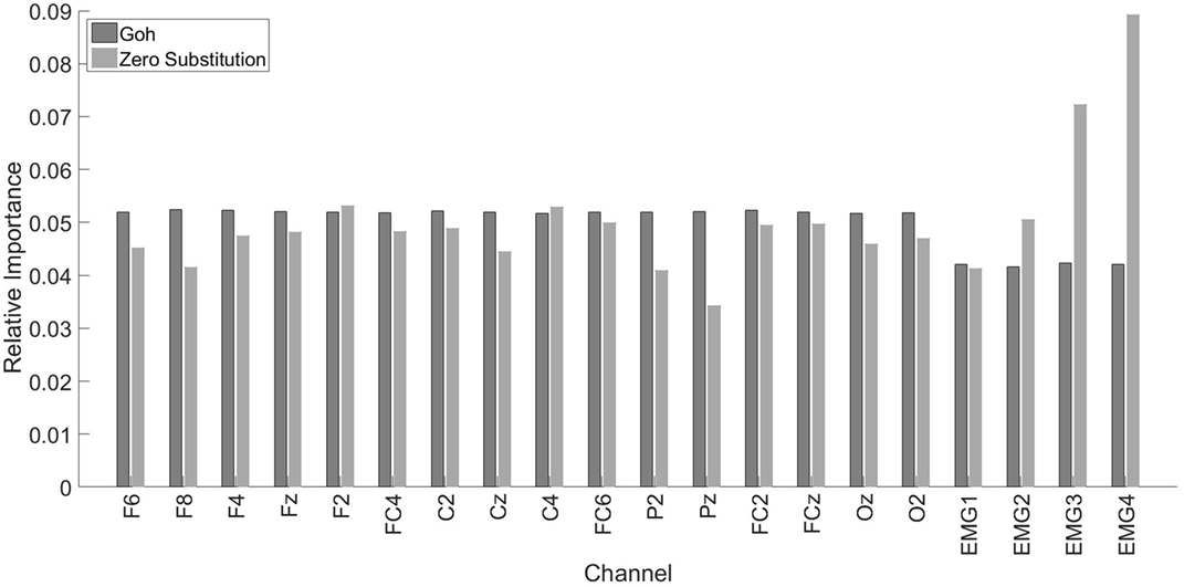
Figure 5. Relative importance for each channel. Dark gray bars represent the results using Goh’s method. The light gray bars represent the Zero Substitution method. MG1, EMG2, EMG3, and EMG4 correspond to the upper trapezius, lower trapezius, deltoideus, and pectoralis major, respectively.

For studying the information carried by different systems (EEG, EMG, time), we used the TSMR_N approaches. In this case, we took into consideration the regression values in the second layer when different configurations were used. Figure 6 presents the accumulated relative importance for the different configurations. In the first configuration, comparing the EEG importance and the EMG importance with a t-test resulted in a p-value <0.001, indicating that the EMG was more important (53%). The values for TSMR₈ were 0.013, 0.017, 0.552, 0.225, 0.077, 0.031, 0.034, 0.016, 0.021, and 0.14 for EEG, EMG, and the eight previously estimated points, respectively. This means that the EEG and EMG were not relevant for the reconstruction of the motion in that configuration. Even from TSMR₂, the added importance of EEG and EMG was only 4.1%.

FIGURE 6

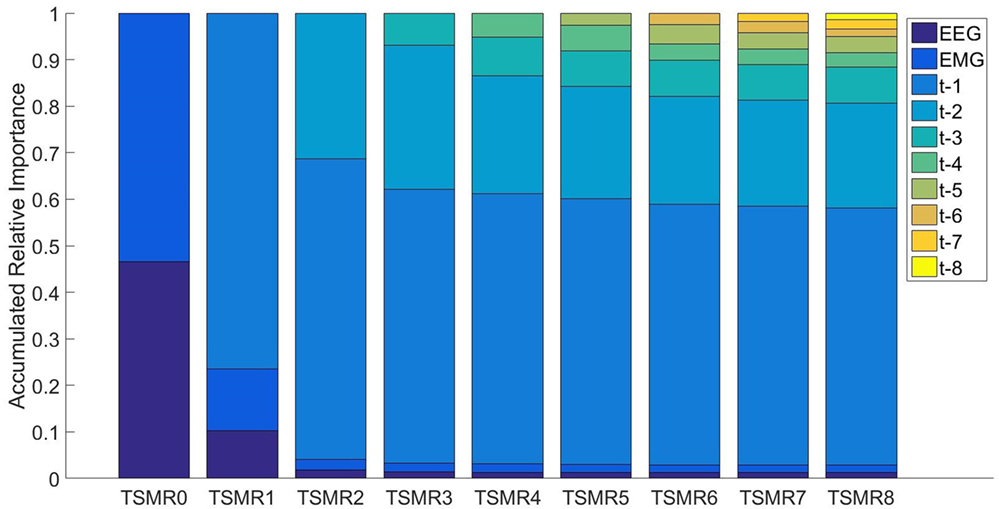
Figure 6. The accumulated relative importance for different configurations of TSMR_N. In the case of TSMR₀, only EEG (darker blue) and EMG (lighter blue) are present. In the rest of the configurations, the added bars correspond to the added time information. For example, in TSMR₁, the bar in the top corresponds to the previous reconstructed point. In the case of TSMR₈, there are eight bars corresponding to the previous reconstructed points plus the EEG and EMG.

We used the Zero Substitution method again to study the importance of each feature (see Figure 7). These results correspond to the mean across all channels, but the results for each independent channel are very similar to the mean, especially in the EEG. The highest value in the EEG is for the first frequency band (1–4 Hz) with a weight of 22.1%, while the minimum corresponds to the second band (5–8 Hz) with a weight of 3.1%. In the case of the EMG, the maximum value corresponds to WAMP with a weight of 16.5%, while the minimum corresponds to SSM with a weight of 1.4%. As a mean value, the EEG has a weight of 5.4% and the EMG of 5.8%, which is coherent with the previous result.

FIGURE 7

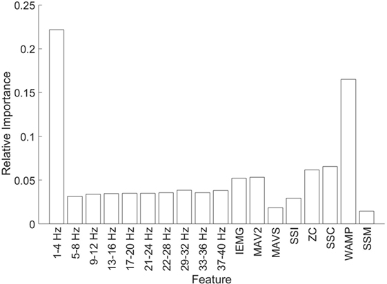
Figure 7. Relative importance for each feature. The first 10 bars correspond to the EEG features, while the last 8 correspond to EMG.

The topological distribution of channel importance, according to the two methods, Zero Substitution and SPoC, is presented in Figure 8. In the case of the Zero Substitution method, the values for the mean correspond to those presented in Figure 5. The SPoC method, similar to the independent component analysis, returns a number of spatial filters equal to the number of variables, in this case 16. For this analysis, we took into consideration only spatial filters with a higher correlation with the output signals.

FIGURE 8

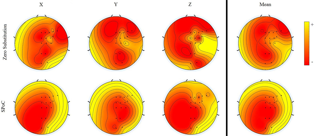
Figure 8. Topographical representation of the variable importance for two different methods. For each method, the importance for the three dimensions and the mean are presented. Each of the methods has different scales. Therefore, the colors in the map are relative to each method.

Discussion

Motion Reconstruction

This study demonstrated that it is possible to reconstruct the hand’s position from non-invasive technologies and without using EMG along the arm. Figure 9 shows the reconstruction using different methods and dimensions. We can see that the reconstruction precision is similar for the three dimensions. In both TCPS₀ and TSMR₀, the reconstructed waveform is similar to the original signal. Nevertheless, in the reconstructed signals, there seem to be noise with high frequency components, which generate most of the error. Considering the low CVs between the speed and the error, the speed does not relate to the error. Using the TSMR₆ shows a softer reconstruction. The high frequency components disappear; instead, the reconstructed waveform is also simpler, showing a more static behavior.

FIGURE 9

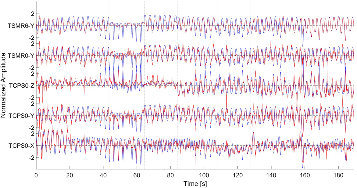
Figure 9. Reconstruction of the signal using different methods. From bottom to top, TCPS₀ for the x dimension, TCPS₀ for the y dimension, TCPS₀ for the z dimension, TSMR₀ for the y dimension, and TSMR₆ for the y dimension. In all the cases, blue lines indicate the original movement and red lines the reconstructed. Dotted vertical lines indicate different phases (described in Figure 1). The amplitude is normalized so it has a mean of zero and SD of 1. The data are from subject #10.

It is important to notice that most of the motions were repetitive in this experiment, i.e., the same motion was repeated several times. This fact, in addition to the importance that the TSMR_N approaches give to the previous estimated steps (Figure 6), leads us to think that the system may be adapting to the repetitive motion, more than the intentions of the subject. Therefore, a real-world application of the same methods may fail to reconstruct the trajectory.

The results of the TCPS_N approaches are not as good as those of the TSMR_N, which is probably due to an over-fitting. Compared with the TSMR_N approaches, the TCPS_N is likely to give a large amount of variable importance to the previously estimated points during the training phase. In the case of the TSMR_N approaches, the temporal information is added in a linear regression layer, i.e., a simpler approach, which is less likely to be over-fitted. Nevertheless, we have to note that using the temporal information helps to reduce the noise in the reconstructed signal. Consequently, a method that efficiently takes into account the previous estimated points should be found.

Information Importance

EEG vs. EMG

The results from Table 1 and Figure 4 suggest that the EEG and EMG systems carry different information, and it is not possible to reach a higher CV without both systems. The results show that the best approach is SMR for 10 out of 16 subjects. Even if the difference between EMS and SMR is not significant, the results in Table 2 suggest that a higher number of subjects may demonstrate so. These results, in addition to those presented in Figure 6, suggest that even if the EMG carries more movement-related information than the EEG, the EEG still provides extra information needed to improve the reconstruction. With the data from Table 1, it might seem that both SMR and CPS are similar predictors, but we can see that SMR is more robust by looking at Table 3. The TSMR_N and TCPS₀ approaches have a higher CV than the state of the art (Lv et al., 2010; Robinson et al., 2013; Kim et al., 2014). In the case of the TCPS_N approaches, the CV values drop considerably (below 0.1), which makes the system completely unusable.

Channel Importance

The analyses that we performed to calculate the channel importance provided different results. Goh’s method shows almost no variation between channels, which is not coherent with other studies (Bradberry et al., 2010). Also, the Zero Substitution method suggests that the EMG has higher importance, coherent with the results already discussed, while Goh’s method suggests the opposite. Altogether, we assume that the Zero Substitution method is more representative of the real channel importance. The results from Goh’s method may come from the theoretical background of such a method. In this case, the only things taken into consideration are the weights of the network. Since every feature has a similar importance for every channel (as discussed for Figure 7), the sum of weights for each channel tends to be the same. Analyzing the importance of each EMG electrode for each dimension shows that there is variation between them. This suggests that the locations of the EMG electrodes are very important, and that using too few or placing them incorrectly, may lead to one of the dimensions not being reconstructed correctly. Therefore, a further study should be done to analyze which are the best positions for the EMG electrodes, and how many are necessary to correctly reconstruct the hand’s position.

Topographical Distribution

We proposed a novel method to calculate the topographical activation and distribution, which provided very different results from the SPoC method. We have to take into consideration that the SPoC method finds linear relations between the EEG signal and the hand’s position, while the Zero Substitution method represents the importance of each channel for the ANN, which is highly non-linear. Thus, the SPoC method shows a more uniform distribution, granting higher importance to the frontal–lateral area than the occipital–middle area. This corresponds to the premotor cortex and the primary motor cortex, as expected. On the other hand, the Zero Substitution method results in a more heterogeneous distribution. In this case, the distribution for x, y, and z dimensions are different among them, each showing an electrode (or group of them) with higher importance than the rest. For the x dimension, the CP3 and the C3 seem to be the most important. For the y dimension, C3 is the most important, while for the z dimension, CP5, C3, and C1 seem to create the most important hub. This kind of result may suggest that different motions are related to different specific parts of the brain. However, in this study, only 16 electrodes were used, and they cover a wide area, from the frontal to the occipital part. A study with a higher density of electrodes should be conducted to see whether the results can be reproduced. In Bradberry et al. (2010), the analysis done with a higher density of electrodes (64) showed different results, whereby CP3 was the most important electrode, but, in this case, the method used for calculating the importance of each electrode is based on a linear model (similar to an autoregressive model).

Features Importance

Finally, we want to focus on the outcome of the analysis of the feature analysis (Figure 7), especially the results regarding the EEG. According to this result, the most important frequency band for predicting the position is 1–4 Hz. This corresponds to the delta waves. Generally, this band is associated with the sleep stage, while the beta band (16–30 Hz) is associated with movement. This relation arises from the increment in the amplitude of such bands during those activities. Nevertheless, it seems that even if there is an increase on the beta bands during the movement, the information of the position is carried on a different band. We also have to take into consideration that the association between bands and activities generally comes from a linear relation, while the Zero Substitution method provides highly non-linear relations. Altogether, we consider that it is possible to use the Zero Substitution method to discover non-linear relations in the EEG that would remain hidden otherwise. The disadvantage of this method is due to the way that AAN works; the reason for those relations is not always clear.

Future Work

There are still many improvements to do in this field to be able to obtain a natural and precise reconstruction of the arm’s movement. In this study, several areas of improvement have been identified. First of all, the training should be changed. At present, the training requires a motion tracking device located on the subject’s hand. If we want to use this system for amputees, this is not possible. Therefore, a training system that does not require the subject to perform a complete real motion is needed. This could be, for example, a digital representation from which the subject can replicate the movement. Second, the use of closed-loop and biofeedback has shown great results in several areas, including BCI (Fernandez-Vargas et al., 2013). Thus, a feedback system should be included in the system to improve the usability and the CV. Finally, in order to gain more knowledge on the underlying processes in the body (both brain and muscle), a higher density of electrodes in both EEG and EMG should be used.

Author Contributions

JF-V contributed in all the stages of the project; experimental design, system preparation, experiments, analysis, and composition. KK was part of the system preparation and the composition of the paper. WY was part of the experimental design and the composition.

Conflict of Interest Statement

The authors declare that the research was conducted in the absence of any commercial or financial relationships that could be construed as a potential conflict of interest.

Acknowledgments

This work was partially supported by JSPS KAKENHI Grant No. 26922011 and 15H05357. We would like to thank Prof. Shaoying Huang of Singapore University of Technology and Design. We also thank Tapio Tarvainen for his help with the proofreading and corrections, Lee Yee Chu for her help in the experiments, and Jorge Femenía for the graphic composition of Figure 1 and proofreading.

References

Au, S., Berniker, M., and Herr, H. (2008). Powered ankle-foot prosthesis to assist level-ground and stair-descent gaits. Neural Netw. 21, 654–666. doi: 10.1016/j.neunet.2008.03.006

PubMed Abstract | CrossRef Full Text | Google Scholar

Blankertz, B., Tomioka, R., Lemm, S., Kawanabe, M., and Müller, K. (2008). Optimizing spatial filters for robust EEG single-trial analysis. IEEE Signal Process. Mag. 25, 41–56. doi:10.1109/MSP.2008.4408441

CrossRef Full Text | Google Scholar

Bradberry, T. J., Gentili, R. J., and Contreras-Vidal, J. L. (2010). Reconstructing three-dimensional hand movements from noninvasive electroencephalographic signals. J. Neurosci. 30, 3432–3437. doi:10.1523/JNEUROSCI.6107-09.2010

PubMed Abstract | CrossRef Full Text | Google Scholar

Cohen, J. (1988). Statistical Power Analysis for the Behavioral Sciences, 2nd Edn. Hillsdale, NJ: Erlbaum.

Google Scholar

Dähne, S., Meinecke, F. C., Haufe, S., Höhne, J., Tangermann, M., Müller, K. R., et al. (2014). SPoC: a novel framework for relating the amplitude of neuronal oscillations to behaviorally relevant parameters. Neuroimage 86, 111–122. doi:10.1016/j.neuroimage.2013.07.079

PubMed Abstract | CrossRef Full Text | Google Scholar

Faul, F., Erdfelder, E., Lang, A. G., and Buchner, A. (2007). G*Power 3: a flexible statistical power analysis program for the social, behavioral, and biomedical sciences. Behav. Res. Methods 39, 175–191. doi:10.3758/BF03193146

PubMed Abstract | CrossRef Full Text | Google Scholar

Fernandez-Vargas, J., Hanns, U. P., Francisco, B. R., and Pablo, V. (2013). Assisted closed-loop optimization of SSVEP-BCI efficiency. Front. Neural Circuits 7:27. doi:10.3389/fncir.2013.00027

PubMed Abstract | CrossRef Full Text | Google Scholar

Fernandez-Vargas, J., Lee, Y. C., Kahori, K., and Yu, W. (2015). “3D continuos hand motion reconstruction from dual EEG and EMG recordings,” in International Conference on Intelligent Informatics and BioMedical Sciences (Okinawa: IEEE), 101–108.

Google Scholar

Fernandez-Vargas, J., Tarvainen, T. V. J., Kita, K., and Yu, W. (2016). “Hand motion reconstruction using EEG and EMG,” in 2016 4th International Winter Conference on Brain-Computer Interface (BCI) (Yongpyong: IEEE), 1–4. doi:10.1109/IWW-BCI.2016.7457457

CrossRef Full Text | Google Scholar

Fisher, R. A. (1925). Statistical Methods for Research Workers. Edinburgh: Genesis Publishing Pvt. Ltd.

Google Scholar

Fukuda, O., Toshio, T., Makoto, K., and Akira, O. (2003). A human-assisting manipulator teleoperated by EMG signals and arm motions. IEEE Trans. Rob. Autom. 19, 210–222. doi:10.1109/TRA.2003.808873

CrossRef Full Text | Google Scholar

Gilja, V., Nuyujukian, P., Chestek, C. A., Cunningham, J. P., Yu, B. M., Fan, J. M., et al. (2012). A high-performance neural prosthesis enabled by control algorithm design. Nat. Neurosci. 15, 1752–1757. doi:10.1038/nn.3265

PubMed Abstract | CrossRef Full Text | Google Scholar

Goh, A. T. C. (1995). Back-propagation neural networks for modeling complex systems. Artif. Intell. Eng. 9, 143–151. doi:10.1016/0954-1810(94)00011-S

CrossRef Full Text | Google Scholar

Gosset, W. S. (1908). The probable error of a mean. Biometrika 6, 1–25. doi:10.2307/2331554

CrossRef Full Text | Google Scholar

Gray, H., and Carter, H. V. (1858). Anatomy: Descriptive and Surgical. London: John W. Parker and Son, West Strand.

Google Scholar

Grosse, P. (2002). EEG–EMG, MEG–EMG and EMG–EMG frequency analysis: physiological principles and clinical applications. Clin. Neurophysiol. 113, 1523–1531. doi:10.1016/S1388-2457(02)00223-7

CrossRef Full Text | Google Scholar

Halliday, D. M., Bernard, A. C., Simon, F. F., and Jay, R. R. (1998). Using electroencephalography to study functional coupling between cortical activity and electromyograms during voluntary contractions in humans. Neurosci. Lett. 241, 5–8. doi:10.1016/S0304-3940(97)00964-6

PubMed Abstract | CrossRef Full Text | Google Scholar

Hashimoto, Y., Ushiba, J., Kimura, A., Liu, M., and Tomita, Y. (2010). Correlation between EEG–EMG coherence during isometric contraction and its imaginary execution. Acta Neurobiol. Exp. (Wars). 70, 76–85.

Google Scholar

Hochberg, L. R., Bacher, D., Jarosiewicz, B., Masse, N. Y., Simeral, J. D., Vogel, J., et al. (2012). Reach and grasp by people with tetraplegia using a neurally controlled robotic arm. Nature 485, 372–375. doi:10.1038/nature11076

PubMed Abstract | CrossRef Full Text | Google Scholar

Horiuchi, Y., Toshiharu, K., Jose, G., and Yu, W. (2009). “A study on classification of upper limb motions from around-shoulder muscle activities,” in 2009 IEEE International Conference on Rehabilitation Robotics, ICORR 2009 (Kyoto: IEEE), 311–315.

Google Scholar

Jung-Hoon, K., and Jun-Ho, O. (2001). “Development of an above knee prosthesis using MR damper and leg simulator,” in Proceedings 2001 ICRA. IEEE International Conference on Robotics and Automation (Cat. No.01CH37164) (Seoul: IEEE), 3686–3691.

Google Scholar

Kiguchi, K., and Hayashi, Y. (2013). “Motion estimation based on EMG and EEG signals to control wearable robots,” in 2013 IEEE International Conference on Systems, Man, and Cybernetics (Manchester: IEEE), 4213–4218.

Google Scholar

Kim, J.-H., Bieβmann, F., and Lee, S.-W. (2014). “Reconstruction of hand movements from EEG signals based on non-linear regression,” in 2014 International Winter Workshop on Brain-Computer Interface (BCI) (Jeongsun-kun: IEEE), 1–3.

Google Scholar

Kruskal, W. H., and Wallis, W. A. (1952). Use of ranks in one-criterion variance analysis. J. Am. Stat. Assoc. 47, 583–621. doi:10.1080/01621459.1952.10483441

CrossRef Full Text | Google Scholar

Leontaritis, I. J., and Billings, S. A. (2007). Input-output parametric models for non-linear systems part i: deterministic non-linear systems. Int. J. Contr. 41, 303–328. doi:10.1080/0020718508961129

CrossRef Full Text | Google Scholar

Liao, X., Dezhong, Y., Dan, W., and Chaoyi, L. (2007). Combining spatial filters for the classification of single-trial EEG in a finger movement task. IEEE Trans. Biomed. Eng. 54, 821–831. doi:10.1109/TBME.2006.889206

PubMed Abstract | CrossRef Full Text | Google Scholar

Lv, J., Li, Y., and Gu, Z. (2010). Decoding hand movement velocity from electroencephalogram signals during a drawing task. Biomed. Eng. Online 9, 64. doi:10.1186/1475-925X-9-64

PubMed Abstract | CrossRef Full Text | Google Scholar

Møller, M. F. (1993). A scaled conjugate gradient algorithm for fast supervised learning. Neural Netw. 6, 525–533. doi:10.1016/S0893-6080(05)80056-5

CrossRef Full Text | Google Scholar

Muller, K. (1989). Statistical power analysis for the behavioral sciences. Technometrics. Available at: http://amstat.tandfonline.com/doi/pdf/10.1080/00401706.1989.10488618

Google Scholar

Phinyomark, A., Hirunviriya, S., Limsakul, C., and Phukpattaranont, P. (2010). “Evaluation of EMG feature extraction for hand movement recognition based on Euclidean distance and standard deviation,” in 2010 International Conference on Electrical Engineering/Electronics Computer Telecommunications and Information Technology (ECTI-CON) (Chiang Mai: IEEE), 856–860.

Google Scholar

Robinson, N., Vinod, A. P., and Guan, C. (2013). “Hand movement trajectory reconstruction from EEG for brain-computer interface systems,” in Proceedings – 2013 IEEE International Conference on Systems, Man, and Cybernetics, SMC 2013 (Manchester: IEEE), 3127–3132.

Google Scholar

Schoffelen, J.-M., Poort, J., Oostenveld, R., and Fries, P. (2011). Selective movement preparation is subserved by selective increases in corticomuscular gamma-band coherence. J. Neurosci. 31, 6750–6758. doi:10.1523/JNEUROSCI.4882-10.2011

PubMed Abstract | CrossRef Full Text | Google Scholar

Seliktar, R., and Kenedi, R. M. (1976). A kneeless leg prothesis for the elderly amputee, advanced version. Bull. Prosthet. Res. 1, 97–119.

PubMed Abstract | Google Scholar

Tabot, G. A., Dammann, J. F., Berg, J. A., Tenore, F. V., Boback, J. L., Vogelstein, R. J., et al. (2013). Restoring the sense of touch with a prosthetic hand through a brain interface. Proc. Natl. Acad. Sci. U. S. A. 110, 18279–18284. doi:10.1073/pnas.1221113110

PubMed Abstract | CrossRef Full Text | Google Scholar

Tenore, F., Ramos, A., Fahmy, A., Acharya, S., Etienne-Cummings, R., and Thakor, N. V. (2007). Towards the control of individual fingers of a prosthetic hand using surface EMG signals. Conf. Proc. IEEE Eng. Med. Biol. Soc. 2007, 6146–6149. doi:10.1109/IEMBS.2007.4353752

PubMed Abstract | CrossRef Full Text | Google Scholar

Waldert, S., Preissl, H., Demandt, E., Braun, C., Birbaumer, N., Aertsen, A., et al. (2008). Hand movement direction decoded from MEG and EEG. J. Neurosci. 28, 1000–1008. doi:10.1523/JNEUROSCI.5171-07.2008

PubMed Abstract | CrossRef Full Text | Google Scholar

Zardoshti-Kermani, M., Bruce, C. W., Kambiz, B., and Reza, M. H. (1995). EMG feature evaluation for movement control of upper extremity prostheses. IEEE Trans. Rehabil. Eng. 3, 324–333. doi:10.1109/86.481972

CrossRef Full Text | Google Scholar

Zuniga, J., Katsavelis, D., Peck, J., Stollberg, J., Petrykowski, M., Carson, A., et al. (2015). Cyborg beast: a low-cost 3d-printed prosthetic hand for children with upper-limb differences. BMC Res. Notes 8:10. doi:10.1186/s13104-015-0971-9

PubMed Abstract | CrossRef Full Text | Google Scholar