Improvement of a Robotic Manipulator Model Based on Multivariate Residual Modeling

1. Introduction

Control of various mechanical systems, such as robotic manipulators, autonomous ground vehicles (AGV), unmanned aerial vehicles (UAV), and surface vehicles (USV), require good model knowledge for precise and efficient control. It has been shown that model-based control is superior to non-model-based equivalent, this, however, requires rigorous mathematical modeling and detailed system analysis in order to develop a good and representative model of the system under consideration. In some cases, a dynamic model can be simple, linear, single input single output (SISO) system, such as a pendulum or mass on a spring [this does not, however, mean that a SISO system is less non-linear than its multiple inputs and outputs (MIMO) equivalent, in fact there is no direct correlation between complexity of the system in terms of non-linearities and its number of inputs and/or outputs]; in others, it may contain many degrees of freedom with MIMO, and have numerous sources of non-linear behavior such as a robotic manipulator, as shown in Figure 1. In the case of a standard industrial 6-DOF manipulator such as ABB IBR140 or KUKA KR150, non-linearities come from multiple sources, some are taken into consideration during model development stages following Lagrangian formulation (Spong et al., 2006; Siciliano et al., 2009). The result of systematic approach in developing a dynamic model is a differential equation governing the motion of a system. For a robotic manipulator, the dynamic model defines the relationship between joint position q_i, angular velocity ${\dot{q}}_i$, and angular acceleration ${\ddot{q}}_i$ to torque τ_i necessary to achieve desired position, velocity, and acceleration.

FIGURE 1

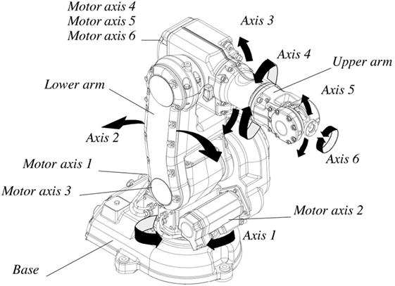
Figure 1. ABB IRB140 industrial manipulator (ABB Robotics, 2004–2009).

However, deductive, first principle models of complex mechanical, chemical, or biological systems lack real world touch. Relying on an incomplete model in general may result in system instability and poor performance. In control engineering, adaptive algorithms allow detrimental effects of unmodelled dynamics to be more or less neutralized over time. However, while we let the computational system correct for the mistakes automatically by the means of feedback, we do not learn what was wrong with the model initially and hence do not correct the original model inductively. Still, this is highly successful. However, with an incomplete dynamic model, the controller needs longer time to discover what is going on in the system to correct it and in some cases it may not be able to do so at all.

In this paper, we focus on investigating the properties of the error signal generated by the internal controller of an industrial robotic manipulator and a model of the same system based on Euler–Lagrange formulation combined with dynamic parameter identification procedure. The discrepancies between two systems, assuming zero measurement noise and ideal conditions is, therefore, the unmodelled dynamics in the theoretical model. To improve the theoretical model, two methods are used: principal component analysis (PCA) and partial least squares regression (PLSR) (Wold, 1985; Helland et al., 1992). PCA is used to test for and reveal structure in the error between the two models, while PLSR is used to modify the initial dynamic equation describing the system. The focus of this particular study is not to improve the output of the real system directly, however, but rather by developing a method by which a more accurate model of the real system can be achieved.

This present paper is a part of an ongoing effort to combine the best of the inductive and the deductive cultures. It has been shown that when a seriously erroneous or incomplete mathematical model is fitted to empirical data, the estimated model parameters may have alias errors. In Martens (2011), the author showed that multivariate subspace modeling of the high-dimensional residuals between measurements and model predictions could give surprisingly detailed quantification of unexpected and thus unmodelled phenomena in the system. It is our goal to improve understanding and mechanistic modeling of a real world system from more in-depth analysis of the residuals between models and measurements. Figures 2, 3, and 7 outline this general approach and intend to give better models, better understanding, and better process control.

FIGURE 2

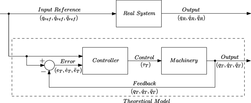
Figure 2. Real system and its theoretical model to be improved.

FIGURE 3

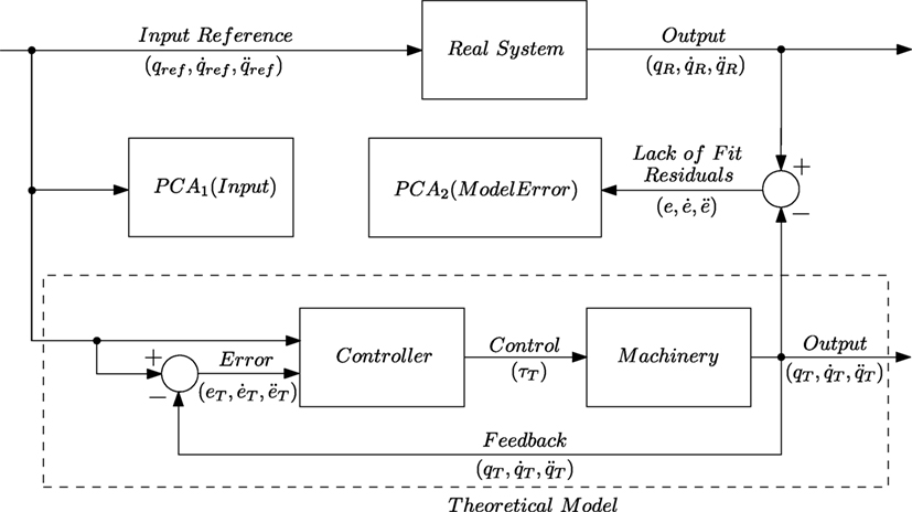
Figure 3. Quality control: PCA of the input and corresponding lack-of-fit residuals.

The first part of this paper outlines in detail the process of developing dynamic model for a rigid body based on first principles described by the basic laws of motion and conservation of momentum, while the second part attempts to improve the quality of the theoretically derived model based on gray box methodology. The initial method is then extended to include data-driven approach as a part of model improvement based on statistical methods.

There are several ways in which the theoretical and data-driven modeling can be combined. Particularly, we focus on using multivariate calibration tools to correct for the errors in the outputs from a mechanistic model. The goal is to improve the estimation of the torque τ needed to control the robotic arm to follow various predetermined trajectories via joint space control. We achieve that by modeling the observed lack-of-fit residual Y between mechanistic model predictions of torque and actual measurements of the “true” torque ${\mathit{\tau }}^{\ast }$ from the desired trajectory specified as position q, velocity $\dot{\mathbf{\text{q}}}$, and acceleration $\ddot{\mathbf{\text{q}}}$ in task space X by a subspace regression methods (Wold, 1985).

The mapping between X and Y is highly non-linear; therefore, we introduce a new version of the PLSR method (PLSR with nominal level representation of the X-variables). This is an extension of the nominal level PLSR used by Martens (2009), in the sense that not only main-effects but also interaction effects are modeled in the nominal level PLSR.

1.1. Dynamic Model Development

For an industrial manipulator as shown in Figure 1, the dynamic model tends to exclude effects, such as friction, gear oil viscosity, and shaft torsion compliance, etc. It is possible to determine some of those effects experimentally, for example a friction model; however, the validity of the model is only over a limited range of motion and conditions, none the less it appears that manufacturers tend to include this in their product. Generally external effects and unmodelled dynamics is treated as an undesirable disturbance and remedied via high gain control action or continuous adaptation in the case of adaptive control strategies.

A definition for a rigid body can be formulated such as a system of particles, which are subjected to some constraints, e.g., holonomic equation (1) where distances between all of the particles remain constant during motion (Goldstein, 1980). The principle of holonomic constraints can be given in a short form as:

$f\left({\mathbf{\text{v}}}_1,{\mathbf{\text{v}}}_2,...{\mathbf{\text{v}}}_n,t\right)=0,$ (1)

where $\mathbf{\text{v}}=d\mathbf{\text{x}}∕\mathit{dt}$, a first derivative of a distance vector x of a particle from some given origin.

One way to visualize a rigid body subjected to holonomic constraints is to imagine a mass that is restrained to move along a predefined path, such as a stiff wire or a double pendulum with masses attached to each of the constant length rigid rods. The issue of the constraints is that the coordinates of the body is no longer independent and the forces acting on the particle because of the constraints are not known a priory (Finn, 2009). The solution to holonomic constraints comes from introduction of a generalized set of coordinates. A system with n particles free to move in all three dimensions is said to have 3n independent degrees of freedom; however, if the system is subject to k holonomic constraints the system is, therefore, reduced to 3n − k independent coordinates (Goldstein, 1980; Spong et al., 2006).

The process of deriving the dynamic model is mathematically involved and relies upon a number of well-known laws and principles of classical mechanics. There are two commonly used approaches to this. The first is the energy based approach and known as Euler–Lagrange formulation, which derived from the principle of virtual work. This formulation has a number of attractive properties for analysis of feedback control system, such as skew symmetry and explicit bounds on the inertia matrix as well as linearity in the inertial parameters. The method is well suited for developing control strategies based on energy and passivity principles (Slotine and Li, 1991; Khalil, 2000). An alternative to the Euler–Lagrange approach is Newton–Euler formulation. The latter method is a recursive formulation for rigid body dynamics and is more suitable for numeric calculations. The Newton–Euler formulation is well suited for real time inverse dynamics calculation and is very well suited for model based control system implementation. The complete derivation procedure is outside of the scope of this paper and will be omitted; however, detailed descriptions are given in Egeland and Gravdahl (2002), Craig (2005), Spong et al. (2006), and Siciliano et al. (2009).

The aim of developing a dynamic model of a rigid body or system of rigid bodies is to derive a set of differential equations that govern time evolution of the systems which is subject to a set of constraints. Systems, such as double pendulum, mass-spring-damper, or a robotic manipulator, are subject to holonomic constraints.

In order to develop a dynamic model, it is necessary to analyze and derive kinematics of a solid object that describes position and velocity of the body in space. As it has been mentioned before, once a set of independent coordinates has been specified, it is then possible to start developing body kinematics based on vector algebra. A rigid body can be described by six independent coordinates, three for position and three for orientation. The transformation from chosen fixed coordinate system in space to a fixed coordinate system attached to a rigid body is known as an orthogonal transformation. A rotation matrix R that fulfils orthogonality conditions r_ijr_ik = δ_jk is called orthogonal and has a number of useful properties, such as R^TR = I, where I is the identity matrix, and R^T = R⁻¹ (Spong et al., 2006; Siciliano et al., 2009). The elementary rotation of a rigid body by some angle in space can be represented as an independent rotation along each of the axis in turn. Composition of rotations is achieved via pre or post multiplication of rotation matrices with coordinate systems attached to intermediate frames of reference. For a two dimensional rotation, the R is a two by two matrix, for a three dimensional rotation the R is a three by three matrix, defining nine r_ij not independent directional cosines. A set of all m × m orthogonal matrices is referred to a Special Orthogonal group of order m and is denoted SO(m) (Khalil and Dombre, 2004; Craig, 2005). The rotation matrix can be parametrized in a number of ways, including Euler angles and quaternions. Rotational transformation only describes rotation of one frame with respect to the other, combination of rotation and translation in a single matrix H defines the homogeneous transformation [equation (2)],

$H=\left[\begin{array}{cc}\hfill \mathbf{\text{R}}\hfill & \hfill \mathbf{\text{d}}\hfill \\ \hfill 0\hfill & \hfill 1\hfill \end{array}\right],$ (2)

where R is 3 × 3 rotation matrix, d is 3 × 1 translation vector.

Once kinematics of a rigid body has been established the forward and inverse kinematic chains for a multi-link robotic manipulator can be developed. Forward and inverse kinematics are seen as a map between two coordinate systems, i.e., joint space vs task space, where the latter is the inverse of the former. The motion of a rigid body through space gives rise to velocity kinematics, which defines description for linear and angular motion. For a robotic manipulator velocity, kinematics provides solution to two types of joint: revolute and prismatic. This in turn defines a manipulator unique Jacobean matrix, which relates linear and angular velocities of the end effector to individual joint velocities.

Armed with the above knowledge manipulator dynamic equation is defined as:

$\mathbf{\text{M}}\left(\mathbf{\text{q}}\right)\ddot{\mathbf{\text{q}}}+\mathbf{\text{C}}\left(\mathbf{\text{q}},\dot{\mathbf{\text{q}}}\right)\dot{\mathbf{\text{q}}}+\mathbf{\text{G}}\left(\mathbf{\text{q}}\right)+\mathbf{\text{F}}\left(\dot{\mathbf{\text{q}}}\right)=\mathrm{\tau },$ (3)

where $\mathbf{\text{M}}\left(\mathbf{\text{q}}\right)\in {\mathbb{R}}^{m\times n}$ is a positive definite inertia matrix, $\mathbf{\text{C}}\left(\mathbf{\text{q}},\dot{\mathbf{\text{q}}}\right)\in {\mathbb{R}}^{m\times n}$ is centrifugal and Coriolis forces matrix, $\mathbf{\text{G}}\left(\mathbf{\text{q}}\right)\in {\mathbb{R}}^{m\times 1}$ is gravitation vector, $\mathbf{\text{F}}\left(\dot{\mathbf{\text{q}}}\right)\in {\mathbb{R}}^{m\times 1}$ is friction vector, $\mathbf{\text{q}},\dot{\mathbf{\text{q}}},\ddot{\mathbf{\text{q}}}\in {\mathbb{R}}^{m\times 1}$ are joint angles, velocity, and acceleration vectors, respectively, and $\mathrm{\tau }\in {\mathbb{R}}^{m\times 1}$ is a vector of actuator torques. Note that the inertia matrix M, centrifugal and Coriolis matrix C, gravity vector G, and friction matrix F are non-linear functions.

The structure of the dynamics in equation (3) is not unique and is also observed in many other mechanical systems such as aerial or ground vehicles and marine vessels.

1.2. Model Parameter Estimation

The difficulty in identification of the dynamic parameters and estimation of forces acting on a mechanical system consisting of a chain of actuated links transcending 0 velocity barrier is due to discontinuity in second derivative. It is safe to say that the forces acting on the joints at near 0 velocity are not fully known, and a high quality description of the dynamics is difficult to come by. More specific studies and methods can be found in Armstrong-Hélouvry et al. (1994) and Olsson et al. (1998).

Most of the advanced control methods require good knowledge of the dynamic model of the plant, performance of a model based control strategy heavily relies on the accuracy of the dynamic parameters of such a model. While adaptive and robust control methods can tolerate some inaccuracies, inverse dynamics, also known as computed torque control in robotic literature, assumes precise knowledge of model parameters in order to achieve near perfect linearization and decoupling of the plant (Khalil, 2000). It is important to note that, even though a manufacturer may have access to majority of manipulator parameters from computer aided design (CAD) models, the dynamic parameters need to be identified and can not be taken directly from CAD or computer aided manufacturing (CAM) system. However, a manufactured and assembled part almost always will have discrepancies with its 3D model due manufacturing tolerances and imperfections; therefore, a fully assembled robotic manipulator will require further identification of parameters and tuning of controller gains. Identification of dynamic parameters requires knowledge of geometric parameters of the manipulator, which has can be achieved following previously described steps.

There are a number of methods and procedures available in engineering and robotics literature on dynamic parameter identification, see An et al. (1986), Gautier et al. (1995), Khalil and Dombre (2004), Siciliano and Khatib (2008), and Ljung (2015), and application of these methods have a fairly and rich history. A good starting point which provides general and solid background on systems identification is given in Ljung (1998).

In Wu et al. (2010), the authors provide an overview of the existing work on dynamic parameter identification methods. There are two main methods for parameter identifications: online and off-line parameter estimation. Each of these methods has an array of sub methods, for example in an online parameter identification adaptive and neural network based strategies received significant amount of attention. For off-line identification of parameters, physical experiments can provide insight into some of the parameter values. It may be necessary to use extra sensors or measuring devices during the experimental work; however, the accuracy of the results depends on the precision of the equipment used. Analysis of input–output data and later minimization of the cost function characterizing the difference between the actual systems output and mathematical model is among the most successful methods for parameter identification as it provides relatively accurate results with relatively easy experimental setup.

Special interest should be given to link inertial parameters as they are important for precise control of motion. As manipulators are designed to kinematic requirements, inertial parameters become a secondary property of the design. From an identification point of view, inertial parameters can be organized in to three groups: fully identifiable, identifiable in linear combinations, and completely unidentifiable according to Atkeson et al. (1986). In the same publication, the authors provide methods for manipulator load and link parameter estimation.

In Swevers et al. (2007a), the authors provide a very comprehensive and detailed description of dynamic model identification for industrial robots. The paper covers all aspects of the process starting from experiment design, data acquisition, parameter estimation, and model validation.

State-space system identification of robot manipulator dynamics was presented in Johansson et al. (2000), where the authors compare a number of commercial software and dedicated subspace model identification software (MOESP) tools in order to evaluate their performance.

In Grotjahn et al. (2001), the authors describe an identification method for industrial robots that does not require the a priori identification of the friction model, which is one of the more difficult tasks. The proposed method relies on weighted least squares (WLS) with the advantage of it being relative simplicity of implementation for standard robot controls and the possibility it provides in identifying unmodelled effects and unnecessary parameters.

An interesting work is done by the authors in Kolyubin et al. (2015). Their approach uses external measurement device, a Nikon K610 optical coordinate measuring machine, together with the KUKA LWR4 + manipulator in an open-loop geometric calibration task. The paper provides a comparative analysis of three different algorithms and two observability indexes used for numerical pose selection and optimization. The planning stage for optimal pose selection used in geometric calibration is done in order to provide better convergence of parameter estimates.

An experimental comparison between the WLS estimation and the extended Kalman filtering (EKF) methods for robot dynamic identification presented in Gautier and Poignet (2001). The application of the proposed methodology is tested on a two-degree of freedom SCARA robot. The advantages and disadvantages of both methods are discussed. The paper concludes that for off-line identification the WLS method with the inverse dynamic model appears to be better than EKF.

Perhaps, more recent and relevant work to this paper has been presented in Gautier et al. (2008) with more detailed information and theory including proofs is given in Gautier et al. (2013). The work is focused on the identification of robotic manipulator dynamic parameters from torque measurements only. The method relies on the assumption that the model and the real system have the same control law, more specifically it requires that the structure and the tuning of the control law is known and implemented in the simulation. In comparison, in this work, no prior knowledge or assumptions are made about control law or the actual structure of the controller used in the real system.

In Janot et al. (2017), authors propose a statistical identification procedure named state dependant parameter (SDP) estimation. The method allows to identify and estimate non-linearities in the dynamic system. The first point worth mentioning is that this method allows graphical representation of the shapes of non-liniarities based on experementally sampled data. The method consists of two stages: first; a non-parametric stage, where the structure of the model representing the system under investigation is identified. The second stage is parametric estimation stage, where the actual parameters of the system is identified. Similar to the presented work here the suggested approach requires minimum of a priori assumptions about non-linearities in the dynamic system. In comparison, the graphical representation of the components extracted during structure decomposition is able to show not only dynamic non-linearites but also other effects on the system caused by external or internal factors.

Once a mathematical model has been developed the next stage is to apply systems identification procedure. In order to estimate internal parameters of the system, applied input vector signals are required to fulfill persistency of excitation (PE) conditions (Boyd and Sastry, 1983; Gorinevsky, 1995; Nikitin, 2007), this guarantees parameter convergence. For a simple pendulum, such input would be a square wave due to its physical properties. For a robotic manipulator, a number of trajectories exists that can give parameter convergence. Initially PE defined a necessary condition for a signal vector consisting of input and the output used for system identification that guaranteed exponential parameter convergence. Later work focused on deriving a set of necessary PE conditions exclusively for input signals that result in PE outputs. The definition and the proof is built upon the identification of a set of necessary conditions for general form of PE function, further expanding on previous results a set of conditions derived for PE input that produces PE states. Finally, efforts are maid to link PE of an input signal to its order of richness (Shimkin and Feuer, 1987). PE is very often studied in connection with adaptive control, systems identification and learning problems and is a rather basic minimum requirement for convergence, this by no means guarantees quality of the results in terms of how well it represents the true parameter values. There are many more things one can do to improve the results. In fact, experimental design is something that is rather overlooked in control engineering world; however, the benefits would be significant. Some previous work can be found in Ng et al. (1977) and Rojas et al. (2007).

In order to satisfy the condition described above, a number of trajectories have been identified and developed based on Fourier series, which have been studied in robotics literature rather extensively, see Swevers et al. (1996, 1997, 2007b) and Park (2006). The actual Fourier series that was used to generate excitation trajectory is given in equation (4). The velocity and acceleration profiles are achieved via differentiating and double differentiating q_f (t).

$\begin{array}{c}{q}_f\left(t\right)=a_0+{\displaystyle \sum _{k=1}^5}\left(a_k\mathit{cos}\left(k\mathrm{\omega }t\right)+b_k\mathit{sin}\left(k\mathrm{\omega }t\right)\right)\hfill \end{array}$ (4)

The other trajectories are a cyclic motion and a move-stop-move trajectory representing continuous periodic motion such as inspection and welding or pick and place, respectively. Selection of parameters for Fourier series is not a straight forward task and care must be taken. The ω parameter defines fundamental or minimum frequency of the series when k = 1, the higher components in the series provide faster dynamics or harmonics. In any electromechanical system achievable velocity and accelerations are limited by the hardware to prevent damage to the equipment. There are current and voltage limiters present in the system meaning that there is a ${\dot{q}}_{\mathit{max}}$ and a ${\ddot{q}}_{\mathit{max}}$, which a joint is able to achieve. In our experience while defining original Fourier set for q extra care must be taken as setting high value for ω will mean that $\dot{\mathbf{\text{q}}}$ and $\ddot{\mathbf{\text{q}}}$ will require lower amplitude defined by a_k and b_k in order not to trigger the over-current protection of the manipulator. Therefore, high initial ω will result in short and fast joint motions meaning the full range for q will not be visited, meaning the trajectory will not be able to excite the system enough to identify all parameters completely. A remedy to this is to either extrapolate and average, which presents issues on its own if there are some manufacturing defects existing outside of the identified parameter range. Alternatively one can select low-enough initial ω, however, amplitudes will have to be higher, meaning that full range of motion in q may not be enough to reach ${\dot{q}}_{\mathit{max}}$ and ${\ddot{q}}_{\mathit{max}}$. It is possible to increase the length of the Fourier series by setting k_max much greater than five, this has a potential problem of exciting natural resonant frequencies of the mechanical system, which will lead to instability and damage to the manipulator. Summarizing, the above can be written in a compact form as such:

$\begin{array}{lll}{\dot{q}}_{f\left(t\right)}\leqq {\dot{q}}_{\mathit{max}}\hfill & \hfill & \\ {\ddot{q}}_{f\left(t\right)}\leqq {\ddot{q}}_{\mathit{max}}\hfill \end{array}$ (5)

One of the useful and interesting properties of the manipulator model given in equation (3) is that it is linear in the parameters (Siciliano et al., 2009), which makes it very suitable for parameter estimation based on least squares method. The alternative form of equation (3) is given below

$\mathrm{\Phi }\left(\mathbf{\text{q}},\dot{\mathbf{\text{q}}},\ddot{\mathbf{\text{q}}}\right)\mathrm{\theta }=\mathrm{\tau }$ (6)

where $\mathrm{\Phi }\in {\mathbb{R}}^{m\times n}$ is the regression matrix with n independent parameters, $\mathrm{\theta }\in {\mathbb{R}}^{n\times 1}$ is a vector of unknown parameters to be identified, $\mathrm{\tau }\in {\mathbb{R}}^{m\times 1}$ is a vector of actuator torques, q, $\dot{\mathbf{\text{q}}}$, $\ddot{\mathbf{\text{q}}}\in {\mathbb{R}}^{m\times 1}$ are vectors of joint angles, velocities, and accelerations, respectively. The formulation of equation (3) in the form of equation (6) makes it very attractive and suitable for parameter identification task. In general it is assumed that the measurements, i.e., joint angles, angular velocities, accelerations, and torques are affected by independent zero-mean Gaussian noise such that

$\begin{array}{l}{q}_m\left(t\right)=q^{\ast }\left(t\right)+e_q\left(t\right)\hfill \\ {\dot{q}}_m\left(t\right)={\dot{q}}^{\ast }\left(t\right)+e_{\dot{q}}\left(t\right)\hfill \\ {\ddot{q}}_m\left(t\right)={\ddot{q}}^{\ast }\left(t\right)+e_{\ddot{q}}\left(t\right)\hfill \\ \mathrm{\tau }\left(t\right)={\mathrm{\tau }}^{\ast }\left(t\right)+e_{\mathrm{\tau }}\left(t\right)\hfill \end{array}$ (7)

where $q^{\ast }$, ${\dot{q}}^{\ast }$, ${\ddot{q}}^{\ast }$, and τ* are ideal measurements. In reality, however, it is rather difficult to measure angular velocity and acceleration, it is generally achieved via differentiation and filtering of the angular position. There are, however, devices that allow for direct measurement of angular velocities called resolvers. It is also possible to use micro electromechanical (MEMS) gyroscopes to measure joint angular acceleration. In the case of industrial manipulators manufacturers such as KUKA or ABB, direct measurement only available for joint angles (ABB Robotics, 2004).

1.3. Model Validation

Once dynamic parameters of a robotic manipulator have been identified it is reasonable to validate the results obtained. There are a number of validation tests that can be carried out on the dynamic model; however, this is a field with limited number of published results and such a validation requires a comprehensive study with solid experimental design methodology behind it. The following suggestions are made in Khalil and Dombre (2004). A direct validation method on the identification trajectory by computing the error vector between the outputs of the real system and the simulation model. This a solid recommendation, however, it is not clear under which conditions one has to establish validation test, i.e., what are the inputs and what are the outputs. An alternative method is to test if the inertia matrix M in equation (3) with identified parameters is positive definite (Spong et al., 2006); this is a simple and straight forward technique, however, it gives no indication of how the identified parameters relate to their true values. At this point it would be of great help to provide some basic guidelines of how to proceed with validation of the dynamic model in control systems sense.

Equation (3) provides the clue, it can be rewritten in terms of $\mathrm{\tau }$ or in terms of $\ddot{\mathbf{\text{q}}}$; therefore, it makes sense to either chose input vector as position q, velocity $\dot{\mathbf{\text{q}}}$ and torque τ, and measure acceleration $\ddot{\mathbf{\text{q}}}$ as the output, or specify input vector as position q, velocity $\dot{\mathbf{\text{q}}}$ and acceleration $\ddot{\mathbf{\text{q}}}$ and measure $\mathrm{\tau }$ as the output.

The model validation should be carried out in a feed-forward, open-loop fashion in order to avoid controller action. In a closed-loop feedback control the regulator will suppress any model uncertainties and it is not possible to make a concrete statement on resulting model quality, as uncertainties in the parameters will be masked by controller actions.

Performance of the model will also depend on the trajectory used for validation. An unstable trajectory will require controller actions, on top of that the system itself must be naturally stable. It is thus not possible to execute a trajectory on a real system, record the torques used, then use those torque series as the only input into the derived simulation model and expect stable and rational behavior at the output. A robotic manipulator is an example of a dual integral system, any discrepancies in initial conditions between two systems will lead to instability of the output.

1.4. Inverse Dynamics Control

A block diagram of typical controller-plant system is given in Figure 2. One of the control schemes that is based on feedback linearization scheme is called inverse dynamics control. In the inverse dynamic control, the input is computed such that it resolves the system in to a set of linear subsystems as in the section above. Computation of such input requires good knowledge of systems parameters, which can be rather difficult to estimate. This is a desirable technique and is often used in conjunction with other methods to increase robustness and stability. The inverse dynamics control assumes perfect knowledge of model parameters and attempts to cancel non-linearities. The system relies on inversion of manipulator inertia matrix M as seen in equation (8) which can be problematic, given the non-linear nature of the model.

$\mathrm{\tau }={\mathbf{\text{M}}}^{-1}\left(q\right)a_q+\mathbf{\text{C}}\left(q,\dot{q}\right)\dot{\mathbf{\text{q}}}+\mathbf{\text{G}}\left(q\right)+\mathbf{\text{F}}\left(\dot{q}\right),$ (8)

where a_q is chosen according to equation (9). In the inverse dynamics or also known as computed torque control, the input signal is calculated according to equation (8), thus by substituting the right hand side of equation (3) with equation (8) reduces to the following double integrator system

$\begin{array}{l}\ddot{q}=a_q\hfill \\ a_q={\ddot{q}}^{\ast }-{\mathbf{\text{K}}}_p\left(q-q^{\ast }\right)-{\mathbf{\text{K}}}_d\left(\dot{q}-{\dot{q}}^{\ast }\right)\hfill \end{array}$ (9)

where K_p and K_d are diagonal gain matrices, and it represents n decoupled subsystems and thus the control law can be designed around a linear second order system. A choice of a_q under closed-loop control is such that initial tracking control task is reduced to stability control around zero in the error space as

$\ddot{e}\left(t\right)+{\mathbf{\text{K}}}_dė\left(t\right)+{\mathbf{\text{K}}}_{p}e\left(t\right)=0$ (10)

where K_p and K_d are proportional and derivative gain matrices, e, $ė$, and $\ddot{e}$ is position, velocity, and acceleration error, respectively. This control method requires access to acceleration measurement, which not always available and in most cases it is derived from position via double differentiation. More details about control method and its applications can be found in Slotine and Li (1991), Spong et al. (2006), Siciliano et al. (2009), and Khalil (2000).

In the scope of this study the control of the dynamic model of the manipulator was chosen to be the one described above. As it has been mentioned it is not always possible to completely cancel all non-linearities and usability of such control scheme on its own is rather unrealistic; however, in the case of a simulation model the knowledge of all of the parameters is readily available. In other words, the identified parameters that establish the simulation model are used in the inverse dynamics controller.

Our interest is not in the analysis and study of the control scheme but rather an attempt to capture lack of fit between mechanistic model and the real system. Therefore, the controller is chosen in such a way to avoid adding extra layer of complexity in transient responses due to controller gains into the error signal. By completely canceling non-linearities inside the simulation via inverse dynamics control and since the model is derived systematically following first principles and identification of dynamic parameters of the real system via system identification procedure, the error signal is thus in its purest form, consisting of only measurements noise and the lack of fit between the models.

1.5. Robotic Manipulator

The mechanical configuration of a typical industrial 6-DOF robotic manipulator arm is such that the first three joints are responsible for the position while the last three, which forms spherical wrist, are responsible for the orientation of the end effector. The actual configuration of the manipulator involved in the study can be seen in Figure 1. There are a number of forces acting on each joint of a robotic arm governed by elementary laws of physics. Two of the main principal forces that a joint’s actuation subsystem has to overcome in order to generate motion is gravitational and friction forces. It is important to note that an electric motor responsible for motion of joint i has to overcome gravity not only affecting its associated link i but all of the successive n − i links.

The robotic system is rather complex, parameter identification procedure is not a straight forward task and requires a large number of equations compared to the actual dynamic parameters to be identified, in Khalil (2000). Robotic manipulators are used in many industries and perform a very wide range of tasks, the control system is complex and tasked not only with providing accurate positioning and tracking but also with rejection of all external disturbances at the same time compensating for natural wear and tear of the mechanical structure. Therefore, the aim is to improve initial theoretical model based on data observation will lead to better, more efficient and longer lasting robotic systems.

2. Multivariate Analysis

Least squares is a well-known method and used in many fields of science and engineering; however, derivative methods like PLSR remains mostly unused in control systems engineering. However, some methods have found its use: proper orthogonal decomposition is used in the sense of model reduction (Hovland and Gravdahl, 2006; Hovland et al., 2008; Benner et al., 2015). There has been very limited research done in application of PCA and PLSR as tools in model improvement and error signal analysis. The model improvement method suggested in this paper in the initial step is based on PCA analysis of the error signal as seen in Figure 2. The assumption is that the error signal between the plant and the model based controller will contain lack of fit between a theoretical model and its data-driven equivalent. The structure of the experimental configuration of both the real system and the equivalent mathematical model is shown in Figure 2. Once the dynamic model of a real system has been developed and a suitable simulation environment has been set up, both of the systems are fed with identical input references. The output at every stage is synchronized and recorded. Once the simulation for a task is complete, the output of both systems is compared and analyzed.

2.1. Experimental Setup

The data for the study were collected from an ABB IRB140 6-DOF robotic manipulator which can be seen in Figure 1. A software simulation model was built based on theoretical modeling of the manipulator. The parameter identification was carried out based on the steps described in the introduction.

A number of trajectories were selected which are representative of a typical robotic manipulator task in an industrial setup, more specifically for this experiment following trajectories were used: continuous cyclic trajectory representing a spray painting operation Figure 5, a pick and place trajectory consisting of relatively short fast moves Figure 4, a welding simulation trajectory similar to pick and place with greater number of segments of motion of the robotic arm, and finally a trajectory consisting of Fourier series typically used in a systems identification task Figure 6.

FIGURE 4

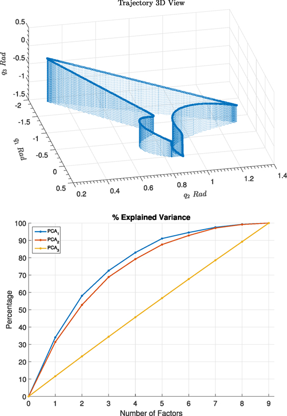
Figure 4. PCA results comparison between input (PCA₁), lack-of-fit residuals (PCA₂) and a random signal (PCA₃) for move–stop–move trajectory.

FIGURE 5

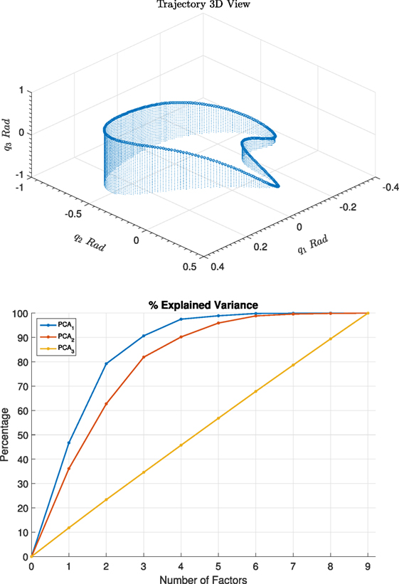
Figure 5. PCA results comparison between input (PCA₁), lack-of-fit residuals (PCA₂) and a random signal (PCA₃) for cyclic trajectory.

FIGURE 6

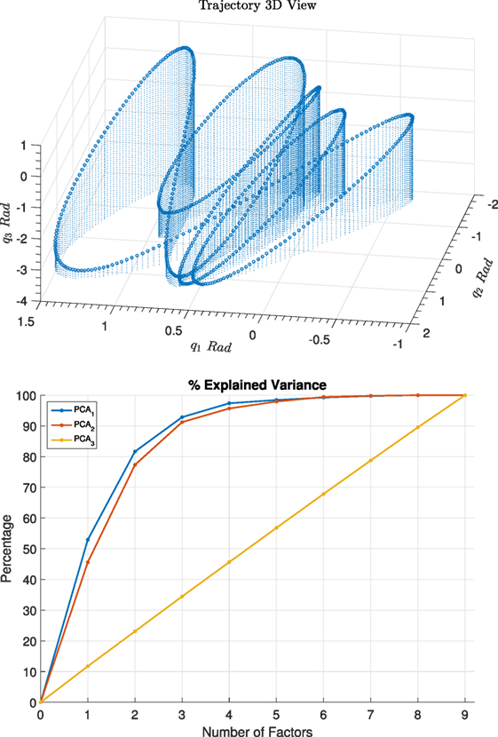
Figure 6. PCA results comparison between input (PCA₁), lack-of-fit residuals (PCA₂) and a random signal (PCA₃) for fourier trajectory.

FIGURE 7

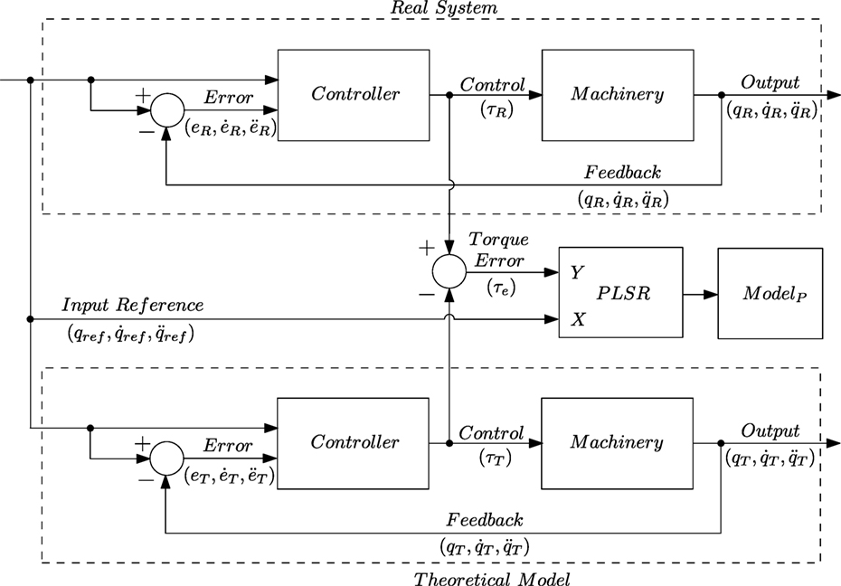
Figure 7. Calibration.

Both the real system and its theoretical software simulation model were fed with identical desired input trajectories, the output of the system was recorded using RobotStudio ^® Signal Viewer. The collected data consist of joint angles and torques is used to perform numerical analysis described in the next section.

The collected data are then organized into vectors and later combined into matrices. The data are organized in such was that each row represents a particular observation at time t, while each column represents a variable such as joint torque or angle.

2.2. Multivariate Analysis Algorithms

Over the years, a number of multivariate analysis (MVA) techniques have been developed and studied in various fields of engineering and science. Such tools established a baseline for analysis of complex data sets, model reduction and response prediction of dynamic systems. The most common and well-known technique called PCA have been rediscovered number of times and is known under different names depending on the field of application. The name PCA is given to a statistical technique which can be implemented using number of workhorse algorithms, such as singular value decomposition (SVD) or eigenvalue decomposition (EVD). PCA is the algorithm of choice for subspace and exploratory data analysis (EDA) given a single data set X with the main objective of discovering major characteristics or structures in the data. The result of a PCA is a set of linearly uncorrelated latent variables each of which is represented in turn by a vector of scores T and loadings P as in:

$\mathbf{\text{X}}={\mathbf{\text{T}}}_a{\mathbf{\text{P}}}_a^T+{\mathbf{\text{E}}}_a$ (11)

Visual inspection of each latent variable, its components and residuals provides a much deeper insight into underlying structural variations in data. An overview of different PCA algorithms and their applications can be found in Wu et al. (1997a), Weingessel and Hornik (2000), Fodor (2002), Wu et al. (1997b), Chatterjee et al. (2000), and Wei-Min and Chein-l (2007). In control systems engineering PCA has found its application mostly, yet not surprising in linear theory and multivariable feedback control design as a measure of controllability and observability as well as model reduction problem (Moore, 1981; Jonckheere, 1984), signal processing (Cabell et al., 2001), etc. PCA is a suitable technique when studying single data set for internal structures or specific characteristics, when it comes to finding a relationship between two data tables PLSR comes to aid. Just like PCA, the technique can be realized using SVD or a power method such as non-linear iterative partial least squares (NIPALS). Mathematically speaking PLSR determines a linear regression model between dependent and independent variables in a new space which accurately describes relationship between them. In both cases in its standard form, assuming that observed data sets contain no missing values the resulting PC’s are orthogonal to each other, this is a very important property for control purposes of MIMO systems via feedback linearization of the plant where decoupling of inputs and outputs is a desirable property (Slotine and Li, 1991). However, in the case where missing values are unavoidable, orthogonality can not be guaranteed and extra steps have to be taken.

2.3. PCA

The field of process control over the years has developed a number of tools able to capture and discover underlying systems dynamics. Tools for multivariate analysis are widely available and have been studied over a long period of time. Algorithms, such as PCA, ICA, PLSR, etc., offer a great deal of features, which makes them suitable for meta-modeling. The most common and well studied algorithm for online process modeling and monitoring is PLSR (Dayal and MacGregor, 1997; Qin, 1998; Ni et al., 2012). Recursive partial least squares (RPLS) algorithm is well suited for both online and off-line batch data analysis, and has demonstrated its versatility in various industries.

A standard PCA algorithm decomposes a data matrix $\mathbf{\text{X\hspace{0.17em}}}\in {\mathbb{R}}^{m\times n}$ in such a way that each principal component contains maximum variance after a_th ∈ [1, …, A] factor:

$\mathbf{\text{X}}={\mathbf{\text{T}}}_a{\mathbf{\text{P}}}_a^T+{\mathbf{\text{E}}}_a$ (12)

where ${\mathbf{\text{T}}}_a\in {\mathbb{R}}^{m\times a}$ is a matrix of scores, ${\mathbf{\text{P}}}_a\in {\mathbb{R}}^{n\times a}$ matrix of loadings and ${\mathbf{\text{E}}}_a\in {\mathbb{R}}^{m\times n}$ are residuals. The optimal number of components can be found using jack-knifing or cross-validation technique (Martens and Martens, 2001). The composition of PCA inputs is defined in equation (13). Prior to analysis, data are mean centered and scaled. If no mean centering is carried out prior to the PCA analysis, the first component will be the mean center of the data, thus mean centering is not essential, however, scaling is, and must be performed.

Manipulator output data were collected from three different types of trajectories. The first trajectory represents continuous cyclic motion of the manipulator as shown in Figure 5. This could be an inspection or painting task on a production line. The second trajectory is of move-stop-move, see Figure 4, type and is typical for packing, sorting, assembly or welding operation of an industrial robot, which is dominant type of activity for robotic manipulator systems currently applied in the industry. The final trajectory is generated from Fourier series, see Figure 6, and is typical for parameter estimation procedure where the system is required to have rich input to guarantee parameter convergence. During the experiment the real system and the simulation model were fed with identical input reference signal, as illustrated in Figures 2 and 3. The input and the error signal were analyzed by PCA independently as shown in Figure 3, the results can be seen in Figures 4–6.

The PCA₁ input matrix consists of the input trajectory, i.e., joint position [q₁, q₂, q₃], velocity $\left[{\dot{q}}_1,{\dot{q}}_2,{\dot{q}}_3\right]$, acceleration $\left[{\ddot{q}}_1,{\ddot{q}}_2,{\ddot{q}}_3\right]$, respectively, while PCA₂ input is the error between the real systems output and theoretical model. PCA₃ is purely for comparison and consists of white noise. Detailed structural description of each row of PCA input X is:

$\begin{array}{lll}{\mathit{PCA}}_1:\mathbf{\text{X}}\in {\mathbb{R}}^{m\times j}=\left[\mathbf{\text{q}},\dot{\mathbf{\text{q}}},\ddot{\mathbf{\text{q}}}\right]\hfill & \hfill & \\ {\mathit{PCA}}_2:\mathbf{\text{X}}\in {\mathbb{R}}^{m\times j}=\left[{\mathbf{\text{e}}}_q,{\dot{\mathbf{\text{e}}}}_q,{\ddot{\mathbf{\text{e}}}}_q\right]\hfill & \hfill & \\ {\mathit{PCA}}_3:\mathbf{\text{X}}\in {\mathbb{R}}^{m\times j}=\left[\mathrm{\omega }{}_1,\mathrm{\omega }{}_2,\mathrm{\omega }{}_3\right],\hfill \end{array}$ (13)

where ${\mathbf{\text{e}}}_q$, ${\dot{\mathbf{\text{e}}}}_q$ and ${\ddot{\mathbf{\text{e}}}}_q$ is the error between measured and estimated value of position, velocity and acceleration, respectively, ${\mathit{\omega }}_1$, ${\mathit{\omega }}_2$, ${\mathit{\omega }}_3$ are white noise vectors used purely for comparison of structured vs unstructured data, see Figures 4–6.

The error between the outputs of two systems is due to the lack of knowledge and lack of modeling effort disregarding sensory noise. It is possible to develop a more comprehensive theoretical model of the real system by taking in to account non-linearities describing friction, drive shaft flexibility, gearbox backlash etc.; however, the complexity of such a model would increase exponentially the more variables taken in to account. Therefore, a natural question arises whether there is anything that can be done about this structure in the error and how can it be used to expand the initial theoretical model to be more representative of the real system. To answer this question, we use PLSR to find the underlying structure in the error signal, such that more accurate prediction is achieved.

2.4. PLSR

PLSR is capable of developing a meta-model of the input–output data. There are several equivalent ways to describe the PLSR model and the algorithm used to develop it. The version used in this work is based on the original version of the algorithm introduced in Wold et al. (1983).

The purpose is to be able to predict a set of j regressand variables of $\mathbf{\text{Y}}\in {\mathbb{R}}^{m\times j}=\left[{\mathbf{\text{y}}}_1,\dots ,{\mathbf{\text{y}}}_j\right]$ from a set of k regressor variables of $\mathbf{\text{X}}\in {\mathbb{R}}^{m\times k}=\left[{\mathbf{\text{x}}}_1,\dots ,{\mathbf{\text{x}}}_k\right]$ via a set of A linear combinations of k X-variables, based on joint observations $\left[{\mathbf{\text{y}}}_i,{\mathbf{\text{x}}}_i\right],\forall i\in \left[1,\dots ,m\right]$ from Y and X respectively.

In general case, the composition of X and Y are time synchronized meaning that each row of the regressor matrix corresponds to an observation taken at the same time interval in the regressand matrix. In other words there is no time discrepancy between input and output data as each row in both matrices represents an observation at a particular time (t). A step ahead time shift can be introduced by shifting the rows of Y matrix while keeping the row of the X unchanged. Thus, by introducing a time shift of (t + 1) inside the regressand Y which contains systems output, from unchanged regressor X which contains systems input trajectory the proposed algorithm builds a model that is able to predict systems output at (t + 1) given the input at time (t), therefore, the joint observations become [y_{i,( t+1)}, x_{i,( t)}]. In the remained of the text the subscript (t + 1) in the in the y_{i,( t+1)} variables and (t) in the x_{i,( t)} variables are omitted for clarity and space consideration; however, all of the results presented are for (t + 1) prediction of the output given the input at time (t). For the validity of matrix operations after time shift in Y, the size of the X must be trimmed to maintain the same number of rows in both matrices.

The general bi-linear regression model, at rank a, may be summarized as follows:

Step 1: estimate and subtract the mean of each of the variable in X and Y.

Step 2: extract weighted combinations ${\mathbf{\text{t}}}_a\in R^{m\times 1}\forall a\in \left[1,\dots ,A\right]$, from X by defining weight vectors ${\mathbf{\text{v}}}_a\in {\mathbb{R}}^{k\times 1}$ so that:

${\mathbf{\text{T}}}_A=\left(\mathbf{\text{X}}-\overline{\mathbf{\text{x}}}\right){\mathbf{\text{V}}}_A,$ (14)

where $\overline{\mathbf{\text{x}}}$ is the mean of each variable of X and each of the columns v_a in the weight matrix V_A are defined according to some criterion, resulting in the orthogonal score matrix ${\mathbf{\text{T}}}_A\in {\mathbb{R}}^{m\times A}=\left[{\mathbf{\text{t}}}_1,\dots ,{\mathbf{\text{t}}}_A\right]$. Different methods rely on different definitions of the weight vectors in V_A In PCA each column vector v_a in V_A is chosen to maximize the variance of each score vector t_a. In PLSR each vector v_a is chosen as to maximize the covariance between the X-score vector t_a and the corresponding linear combination of the Y-variable.

Step 3: for each rank $a\in \left[1,\dots ,A\le \mathit{min}\left(n-1,k\right)\right]$ (for general case matrix rank should be used), approximate X and Y according to the bi-linear regression structure model:

$\begin{array}{lll}\mathbf{\text{X}}=\overline{\mathbf{\text{x}}}+{\mathbf{\text{T}}}_A{\mathbf{\text{P}}}_A^T+{\mathbf{\text{E}}}_A\hfill & \hfill & \\ \mathbf{\text{Y}}=\overline{\mathbf{\text{y}}}+{\mathbf{\text{T}}}_A{\mathbf{\text{Q}}}_A^T+{\mathbf{\text{F}}}_A\hfill \end{array}$ (15)

Loadings are estimated, e.g., by projection [ordinary least squares (OLS) regression]:

$\begin{array}{lll}{\mathbf{\text{P}}}_A^T={\left({\mathbf{\text{T}}}_A^T{\mathbf{\text{T}}}_A\right)}^{-1}{\mathbf{\text{T}}}_A^T\mathbf{\text{X}}\hfill & \hfill & \\ {\mathbf{\text{Q}}}_A^T={\left({\mathbf{\text{T}}}_A^T{\mathbf{\text{T}}}_A\right)}^{-1}{\mathbf{\text{T}}}_A^T\mathbf{\text{Y}}\hfill \end{array}$ (16)

In practice, the optimal number of PLS components (PCs) A = A_opt ∈ [1: min( j, k)] is determined either manually, by jack-knifing, cross-validation, or other methods (Martens and Martens, 2001), leaving the unmodelled residuals

$\begin{array}{lll}{\mathbf{\text{E}}}_A=\overline{\mathbf{\text{X}}}-{\mathbf{\text{T}}}_A{\mathbf{\text{P}}}_A^T\hfill & \hfill & \\ {\mathbf{\text{F}}}_A=\overline{\mathbf{\text{Y}}}-{\mathbf{\text{T}}}_A{\mathbf{\text{Q}}}_A^T,\hfill \end{array}$ (17)

where $\overline{\mathbf{\text{X}}}$ indicates X with mean value removed as shown below

$\begin{array}{lll}\overline{\mathbf{\text{X}}}=\mathbf{\text{X}}-\overline{\mathbf{\text{x}}}\hfill & \hfill & \\ \overline{\mathbf{\text{Y}}}=\mathbf{\text{Y}}-\overline{\mathbf{\text{y}}}.\hfill \end{array}$ (18)

In PLSR, the weight matrix V_A for the first a components is defined as follows, to maximize the explained X–Y covariance: for each component, a = [1, …, A], let w_a be the eigenvector corresponding to the largest eigenvalue in the residual covariance expression remaining after subtraction of the previous a − 1 components, $\left({\mathbf{\text{E}}}_{a-1}^T{\mathbf{\text{F}}}_{a-1}{\mathbf{\text{F}}}_{a-1}^T{\mathbf{\text{E}}}_{a-1}\right)$. Collect these a so-called loading weights vectors in an orthonormal matrix W_A = [w₁, …, w_A]. The weight matrix is then defined as:

${\mathbf{\text{V}}}_A={\mathbf{\text{W}}}_A{\mathbf{\text{G}}}_A,$ (19)

where the bi-diagonal matrix is

${\mathbf{\text{G}}}_A={\left({\mathbf{\text{P}}}_A^T{\mathbf{\text{W}}}_A\right)}^{-1}$ (20)

The prediction of ${\mathbf{\text{y}}}_i\in {\mathbb{R}}^{1\times j}$ from ${\mathbf{\text{x}}}_i\in {\mathbb{R}}^{1\times k}$ in new objects or points in time i, may be attained by

$\begin{array}{l}{\mathbf{\text{t}}}_i=\left({\mathbf{\text{x}}}_i-\overline{\mathbf{\text{x}}}\right){\mathbf{\text{V}}}_A\hfill \\ {\widehat{\mathbf{\text{y}}}}_i=\overline{\mathbf{\text{y}}}+{\mathbf{\text{t}}}_i{\mathbf{\text{Q}}}_A^T\hfill \end{array}$ (21)

with the additional modeling (good for outlier detection and graphical interpretation):

$\widehat{\mathbf{\text{x}}}=\overline{\mathbf{\text{x}}}+{\mathbf{\text{t}}}_i{\mathbf{\text{P}}}_a^T$ (22)

$\begin{array}{l}{\mathbf{\text{e}}}_i={\mathbf{\text{x}}}_i-{\widehat{\mathbf{\text{x}}}}_i\hfill \\ {\mathbf{\text{f}}}_i={\mathbf{\text{y}}}_i-{\widehat{\mathbf{\text{y}}}}_i\hfill \end{array}$ (23)

Alternatively, an equivalent short-cut prediction, without explicit modeling of x_i, is:

${\widehat{\mathbf{\text{y}}}}_i={\mathbf{\text{b}}}_{0,A}+{\mathbf{\text{x}}}_i{\mathbf{\text{B}}}_A$ (24)

where estimated rank a regression coefficients are:

${\mathbf{\text{B}}}_A={\mathbf{\text{V}}}_A{\mathbf{\text{Q}}}_A^T$ (25)

with offset vector:

${\mathbf{\text{b}}}_{0,A}=\overline{\mathbf{\text{y}}}-\overline{\mathbf{\text{x}}}{\mathbf{\text{B}}}_A$ (26)

${\mathbf{\text{f}}}_i={\mathbf{\text{y}}}_i-{\widehat{\mathbf{\text{y}}}}_i$ (27)

The structure of each row and column in X and Y is defined as:

$\begin{array}{lll}\mathbf{\text{Y}}\in {\mathbb{R}}^{m\times i}=\left[e_{{\mathrm{\tau }}_1},e_{{\mathrm{\tau }}_2},e_{{\mathrm{\tau }}_3}\right]\hfill & \hfill & \\ \mathbf{\text{X}}\in {\mathbb{R}}^{m\times j}=\left[q_1,q_2,q_3,{\dot{q}}_1,{\dot{q}}_2,{\dot{q}}_3,{\ddot{q}}_1,{\ddot{q}}_2,{\ddot{q}}_3\right],\hfill \end{array}$ (28)

where $e_{{\mathrm{\tau }}_i}$ is the error of an i^th joint between the real system measured torque output and the torque computed by the controller in the simulation model, [q₁, q₂, q₃] are joint reference positions, $\left[{\dot{q}}_1,{\dot{q}}_2,{\dot{q}}_3\right]$ reference velocities and $\left[{\ddot{q}}_1,{\ddot{q}}_2,{\ddot{q}}_3\right]$ reference accelerations, respectively.¹

2.5. Validation Methods for PLSR

It is important that the results from data-driven method such as PLSR or in fact any other estimation procedures are validated and evaluated quantitatively for quality. One can identify two types of validation: internal and external. The external validation is aimed at assessing the resulting model’s ability to generalize, to some extent this can be done from visual examination of the results produced, as the method is able to provide graphical representation of the dominating patters in the model via inspection of scores and loadings. The internal validity is assessed by inspecting statistical relevance and performance of modeling results.

The residuals E_A, F_A from estimation of X and Y after A components, respectively can be summarized in terms of root mean square error (RMSE), these summaries in turn can be separated in to calibration residuals RMSEC and prediction or validated residuals RMSEV (in some literature it is abbreviated as RMSEP). The prime use of RMSEC is for the diagnostics purposes in analysis of complex data sets. The RMSEV provides information on model generalization ability and gives an insight into long term error prediction.

In this study three types of cross-validation (CV) methods were carried out: cross trajectory, systematic and random. In each one of the CV technique employed the process is the more or less the same. The full observation data set X and Y is split in to a number of subsets. In a full leave-one-out cross-validation a single sample is taken out and kept hidden. The model is trained without the hidden sample, after the initial training the generated model is used to predict the hidden sample. The process is repeated for every sample, and therefore, the number of validation runs is equal to the number of samples in the set. This presents a problem for large data sets with many observations like in this case where samples are taken at high frequency resulting in matrices X and Y with thousands of rows.

The use of CV allows to determine the optimal number of components A_opt to be employed in the final model. It provides a good estimation of model ability to generalize, i.e., the predictive ability. Cross-validation combined with jack-knifing allows to identify variables that least affect the model, in other words it allows estimation of a parameter reliability. Finally, it provides tools for outlier identification and detection of abnormality.

2.5.1. Cross Trajectory Validation

In cross trajectory validation routine the data set is split in to subsets that correspond to each trajectory. The model is trained with one trajectory removed at a time. The resulting model is used to predict the hidden trajectory.

2.5.2. Systematic Cross-Validation

In systematic CV the full data set is broken in to a number of subsets. In this study, the number of blocks for systematic and random methods was chosen to be 20. The choice for the number of validation blocks depends on the amount of data available and the system under consideration. In systematic validation routine each hidden block contains sequential rows. The process is repeated a number of times equal to the number of validation blocks.

2.5.3. Random Cross-Validation

During random cross-validation just as in systematic the full data set is split in to a number of subsets; however, in the case of random method each row in the hidden block has little correlation to its neighbor as during row selection each is selected randomly from the full set.

In general, the higher the choice of validation blocks the closer it gets to full leave-one-out method. The RMSEV for Y is calculated as the average of RMS of the validation subsets.

2.6. PLSR Modification

Results from application of a standard PLSR method are shown in Figures 8 and 9. The comparison between using no compensation method, standard PLSR and modified PLSR as suggested later in this paper is shown in Table 1 and confirms that the overall improvements are insignificant and it is clear that one has to look further than a standard method.

FIGURE 8

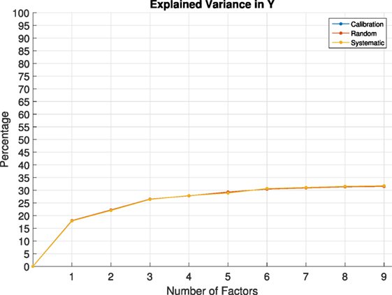
Figure 8. Standard PLSR results.

FIGURE 9

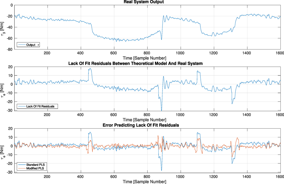
Figure 9. Illustrative result to complement Table 1.

TABLE 1

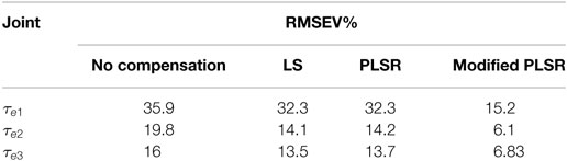
Table 1. 20-fold cross-validation (random block selection) for PLSR predicting ${\mathrm{\tau }}_e$ from q, $\dot{\mathbf{\text{q}}}$, $\ddot{\mathbf{\text{q}}}$ for all trajectories.

The quality of the model developed by PLSR was assessed using:

$\mathit{RMSE}=\frac{\parallel {\mathbf{\text{Y}}}^{\ast }-\widehat{\mathbf{\text{Y}}}{\parallel }_2}{\parallel {\mathbf{\text{Y}}}^{\ast }{\parallel }_2},$ (29)

where Y* is matrix of observations collected from the real system as in equation (28), $\widehat{\mathbf{\text{Y}}}$ is the results from PLSR compensated model. The same formula is used to test for model quality between the real system and the theoretical model.

The problem lays in non-linearity of the system that generates the error signal itself. The dynamic model developed earlier attempts to cancel well known non-linearities in the model by inverting them, in this case it is a well established and realizable solution. However, the more complex non-linearities present in the system in the form of friction around 0 velocity, backlash in the gearbox, etc. are not compensated due to complexity and effort required. In order to address some of the issues two effective modifications to the algorithm are proposed. The modification takes two steps and is concerned with preprocessing the data before it is fed into PLS. Figure 13 shows block diagram representation of the modified PLSR calibration scheme.

2.6.1. Step 1

Each of the X variables is replaced by a nominalized representation of itself. This is better described by the concept of quantization: nominalization expansion is achieved by discretizing the operational range of the variable in to a number of equally spaced levels, thus defining a nominalization level. Each individual level is then expanded in to a separate column. If a variable falls in to the range of the nominal block m it is marked as 1 else it is replaced by 0. For example, given a single vector $\mathbf{\text{q\hspace{0.17em}}}\in {\mathbb{R}}^{m\times 1}$ applying nominalization expansion of level-k will result in a new matrix ${\mathbf{\text{X}}}_q\in {\mathbb{R}}^{m\times k}$.

2.6.2. Step 2

Replace the nominalized matrix X_q by a matrix of interaction effects across variables. At this point each column of the X_is replaced according to

${\widetilde{\mathbf{\text{X}}}}_{m\times p}=\left\{{\mathbf{\text{X}}}_{m\times i}\circ {\mathbf{\text{X}}}_{m\times j}\forall i\in \left\{1:n-1\right\};j\in \left\{i+1:n\right\}\right\},$ (30)

where, X is an input matrix with m rows and n columns, “∘” is defined as the Hadamard product, more commonly known as an element wise product. The resultant matrix $\widetilde{\mathbf{\text{X}}}$ has the same number of rows as the initial matrix X, while number of columns p is equal to (n − 1)n/2 and represents purely interaction effects between variables of the initial input matrix.

The two steps described above provide good improvements to the model derived by PLSR from observational data judging from the results. Finally once a data-driven PLSR model has been developed and cross validated, it is suitable for real time implementation as it can be realized via a look up table of coefficients each corresponding to a particular location in the state space map giving necessary model corrections.

In the case of the experimental data initial matrix $\mathbf{\text{X}}\in {\mathbb{R}}^{m\times 9}\Rightarrow \mathbf{\text{X}}\in {\mathbb{R}}^{m\times 198}$ by applying nominalization level of 22. This value is taken from Figure 12 and depends on the choice of computational time and required accuracy of the final model. In general the optimal nominalization level depends on each case individually and on requirements at hand. It is important to note that the maximum nominalization level is limited by the sensors own discretization scheme. Further study is required to find a mathematical method of establishing an optimal nominalization level without going through experimental trials. Trials were carried out for different nominalization levels, the results can be seen in Figure 12.

3. Model Modification

The initial dynamic model equation (3) can be modified in the following manner without compromising input-output decoupling:

$\mathbf{\text{M}}\left(\mathbf{\text{q}}\right)\ddot{\mathbf{\text{q}}}+\mathbf{\text{C}}\left(\mathbf{\text{q}},\dot{\mathbf{\text{q}}}\right)\dot{\mathbf{\text{q}}}+\mathbf{\text{G}}\left(\mathbf{\text{q}}\right)+\mathbf{\text{F}}\left(\dot{\mathbf{\text{q}}}\right)+\mathbf{\text{B}}{f}_{\mathit{pls}}\left(\mathbf{\text{q}},\dot{\mathbf{\text{q}}},\ddot{\mathbf{\text{q}}}\right)=\mathrm{\tau },$ (31)

where B is PLSR coefficients and f_pls is a function that transforms the raw sensor data according to nominalization rules and applies interactions. Figures 13 and 11 show block diagram representation of the model modification scheme. At first PLSR model is calibrated as seen in Figure 13 and once adequate level of performance is achieved it is used in prediction stage as displayed in Figure 11.

FIGURE 10

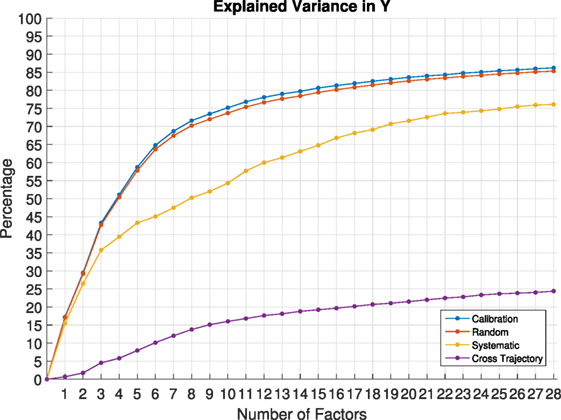
Figure 10. Modified PLSR results. Comparison of various cross-validation methods.

FIGURE 11

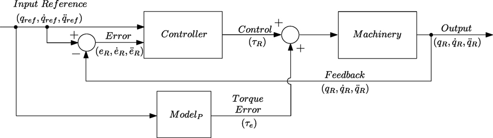
Figure 11. Prediction.

FIGURE 12

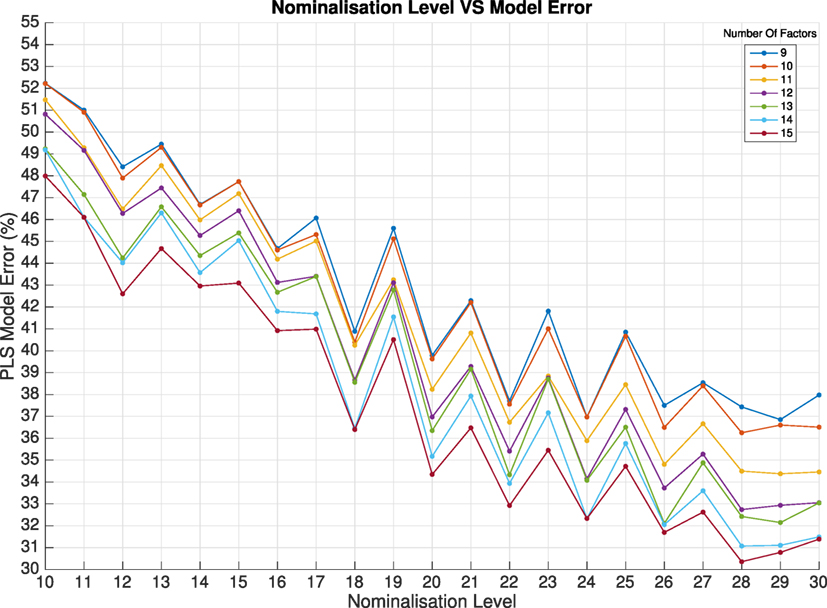
Figure 12. Nominalization level vs model error.

FIGURE 13

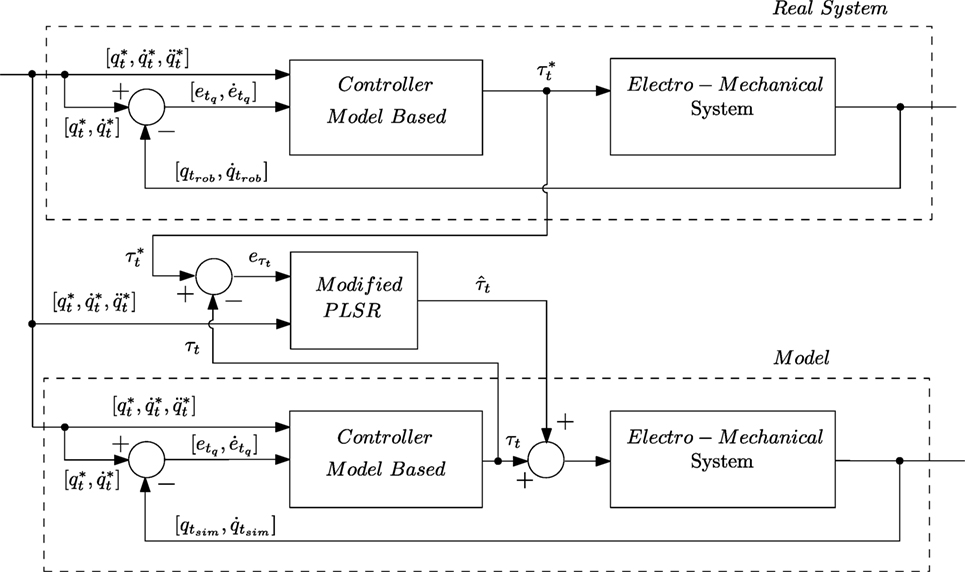
Figure 13. Detailed PLSR modifications: calibration.

4. Results

The results of calibration and cross-validation of the modified PLSR method is shown in Figure 10. Three different cross-validation schemes were used to test the model. (1) Random cross-validation scheme splits the model in to n number of blocks of randomly selected rows from X and Y, the block is then removed from training set, the model is calibrated and the resulting B coefficients are used to predict unseen Y from unseen X. (2) Systematic cross-validation scheme sequentially splits X and Y in to n blocks, each time a block is taken away and model is calibrated, the resulting B coefficients, similarly to the random cross-validation scheme are used to predict unseen blocks of X and Y. (3) Finally cross trajectory validation is performed. Cross trajectory validation is a subset of systematic validation, with the number of blocks equal to the number of experiments carried out, in this case it was three. This type of cross-validation will give the least accurate results, which is no surprise as the model is not capable of predicting completely unseen situations.

Finally, from a control systems engineering point of view it is interesting to see how this method and the results can improve on the dynamic model of the manipulator by closing the gap between the real system and the dynamic model that was derived using first principles. For this to happen, the results from the PLSR methodology has to be integrated into standard dynamic model framework. Looking at the structure of dynamic equation (3) one can see that it can be viewed as a function that provides mapping between a set of q, $\dot{\mathbf{\text{q}}}$ and $\ddot{\mathbf{\text{q}}}$ on one side, and $\mathrm{\tau }$ on the other. Therefore, the model developed using PLSR should also be a map between the space spanned by q, $\dot{\mathbf{\text{q}}}$ and $\ddot{\mathbf{\text{q}}}$ to space spanned by $\mathrm{\tau }$. This can be achieved by carefully selecting Y matrix variables. The resulting B coefficients will provide mapping according to specified PLS regression inputs. However, in order to modify the dynamic model in line with linearization and decoupling properties of the inverse dynamics which results in a set of decoupled liner subsystems one has to make sure that the results of the PLSR do not violate this property. The results can be seen in Figure 9.

The torque signal may appear to be noisy; however, it is important to understand the electromechanical system of joint control before making conclusive remarks regarding the source of vibration visible on Figure 9. The torque is generated using high power IGBT transistors which control current in three phase permanent magnet synchronous motors (PMSM) (Drives, 2011). For the ABB IRB140 manipulator the encoder is coupled with the electrical motor shaft and is located at the back of the electrical drive. The electrical motor is coupled to a reduction gearbox which acts as a mechanical low pass filter; however, it does introduce dynamics into the system via internal friction and backlash just to name a few effects. Around zero velocity crossing these effects become significant and the whole field of study called tribology exists studying various phenomena caused by surface interactions, which includes friction, lubrication and wear. The torque measurement comes from electrical amplifier driving the motors and the source of jitter can be related to current fluctuations, resonance of the system operating a particular trajectory or meshing gears of the gearbox. A more detailed and focused investigation is necessary to provide certain answers for the observed phenomenon and is outside the scope of this paper.

The drawback of the currently suggested method in this paper is that the size of initial X is increased dramatically requiring large amount of memory to process the data. However, using sparse PLSR (Chun and Keles, 2010) instead of conventional PLSR could remedy this. Moreover, given the current state of the hardware this is not a problem for off-line analysis and model improvements. The other drawback of this method is that it relies too much on state space being visited at least once, the state space that has not been visited during calibration stage will have model parameters and further improvements are necessary; however, there is a number of options are available to remedy this, for instance, a pyramidal representation of nominal levels at different discretization levels could probably allow for sensible interpolation in regions of the state space not properly sampled.

5. Conclusion

In this paper, we have investigated a possibility of dynamic model improvement based on the well established statistical analysis methods PCA and PLSR in the hope of bridging the gap between purely mechanistic and purely data-driven modeling. Unlike similar data driven modeling techniques such as ANN, PLSR and PCA provides an open book approach to the knowledge gained. By analyzing scores and loadings plots it is possible to gain an deep understanding into the dynamics of the system and develop steps necessary to improve current modeling and estimation tools. The initial PLSR data-driven model has shown very little improvement; however, nominalization and interaction expansion of the X matrix provided significant improvements. The methodology developed allows for a step ahead error compensation. The method, however, requires further work in order to make it applicable for real time implementation.

Author Contributions

SG had the original idea and performed majority of work described in the publication. HR provided support in algorithms and Matlab code for model simulation. JG supervised during the project and advised on control theory and robotics. HM provided support in theory development and regression algorithms.

Conflict of Interest Statement

The authors declare that the research was conducted in the absence of any commercial or financial relationships that could be construed as a potential conflict of interest.

Acknowledgments

Stepan Pchelkin for his help in experimental setup and data acquisition, Sergei Kolyubin for the fruitful discussions and input during this research.

Funding

This work is performed in Next Generation Robotics for Norwegian Industry. The project is funded by the Research Council of Norway, Statoil AS, Hydro AS, Tronrud Engineering AS, SbSeating AS, Glen Dimplex Nordic AS, and RobotNorge AS. SINTEF and the Norwegian University of Science and Technology are research partners.

Footnote

1. ^Only the first three joints out of six of the manipulator were used in this study. The first three joins responsible for position of the end effector in task space, while last three are responsible for orientation of the end effector.

References

ABB Robotics. (2004). Prod.man 140 Proc/Ref info. ABB Automation Technologies AB. en/m2000,m2000a,m2004 edition. 3HAC023297-001.

Google Scholar

ABB Robotics. (2004–2009). Product Manual. IRB 140 Typ C; IRB 140T Typ C; IRB 140-6/0.8 Typ C; IRB 140T-6/0.8 Typ C. document id: 3hac027400-001 Revision: E edn. ABB Automation Technologies AB.

Google Scholar

An, C., Atkeson, C., and Hollerbach, J. (1986). “Estimation of inertial parameters of rigid body links of manipulators,” in Proceedings of the 24th IEEE Conference on Decision and Control, 990–995.

Google Scholar

Armstrong-Hélouvry, B., Dupont, P., and Canudas-De-Wit, C. (1994). A survey of models, analysis tools and compensation methods for the control of machines with friction. Automatica 30, 1083–1138. doi: 10.1016/0005-1098(94)90209-7

CrossRef Full Text | Google Scholar

Atkeson, C. G., An, C. H., and Hollerbach, J. M. (1986). Estimation of inertial parameters of manipulator loads and links. Int. J. Rob. Res. 5, 101–119. doi:10.1177/027836498600500306

CrossRef Full Text | Google Scholar

Benner, P., Gugercin, S., and Willcox, K. (2015). A survey of projection-based model reduction methods for parametric dynamical systems. SIAM Rev. 57, 483–531. doi:10.1137/130932715

CrossRef Full Text | Google Scholar

Boyd, S., and Sastry, S. (1983). On parameter convergence in adaptive control. Syst. Control Lett. 3, 311–319. doi:10.1016/0167-6911(83)90071-3

CrossRef Full Text | Google Scholar

Cabell, R., Palumbo, D., and Vipperman, J. (2001). “A principal component feedforward algorithm for active noise control: flight test results,” in IEEE Transactions on Control Systems Technology, Vol. 9, 76–83.

Google Scholar

Chatterjee, C., Kang, Z., and Roychowdhury, V. P. (2000). “Algorithms for accelerated convergence of adaptive PCA,” in IEEE Transactions on Neural Networks, Vol. 11, 338–355.

Google Scholar

Chun, H., and Keles, S. (2010). Sparse partial least squares regression for simultaneous dimension reduction and variable selection. J. R. Stat. Soc. Series B Stat. Methodol. 72, 3–25. doi:10.1111/j.1467-9868.2009.00723.x

PubMed Abstract | CrossRef Full Text | Google Scholar

Craig, J. (2005). “Introduction to robotics: mechanics and control,” in Addison–Wesley Series in Electrical and Computer Engineering: Control Engineering (Pearson/Prentice Hall).

Google Scholar

Dayal, B. S., and MacGregor, J. F. (1997). Recursive exponentially weighted {PLS} and its applications to adaptive control and prediction. J. Process Control 7, 169–179. doi:10.1016/S0959-1524(97)80001-7

CrossRef Full Text | Google Scholar

Drives, A. B. B. (2011). Electrical Braking Technical Guide No. 8, 8th Edn. ABB Automation Technologies AB. 3AFE6436252534 REV B EN 6.5.2011.

Google Scholar

Egeland, O., and Gravdahl, J. T. (2002). Modeling and Simulation for Automatic Control. Trondheim, Norway: Marine Cybernetics, 76.

Google Scholar

Finn, J. (2009). “Classical mechanics,” in Engineering Series (Jones & Bartlett Learning).

Google Scholar

Fodor, I. K. (2002). “A survey of dimension reduction techniques,” in Technical Report (U. S. Department of Energy, Lawrence Livermore National Laboratory).

Google Scholar

Gautier, M., Janor, A., and Vandanjon, P. O. (2008). “Didim: a new method for the dynamic identification of robots from only torque data,” in IEEE International Conference on Robotics and Automation, 2122–2127. doi:10.1109/ROBOT.2008.4543520

CrossRef Full Text | Google Scholar

Gautier, M., Janot, A., and Vandanjon, P. O. (2013). A new closed-loop output error method for parameter identification of robot dynamics. IEEE Trans. Control Syst. Technol. 21, 428–444. doi:10.1109/TCST.2012.2185697

CrossRef Full Text | Google Scholar

Gautier, M., Khalil, W., and Restrepo, P. P. (1995). “Identification of the dynamic parameters of a closed loop robot,” in Proceedings of 1995 IEEE International Conference on Robotics and Automation, 3045–3050.

Google Scholar

Gautier, M., and Poignet, P. (2001). Extended kalman filtering and weighted least squares dynamic identification of robot. Control Eng. Pract. 9, 1361–1372. doi:10.1016/S0967-0661(01)00105-8

CrossRef Full Text | Google Scholar

Goldstein, H. (1980). “Classical mechanics,” in Addison–Wesley Series in Physics (Addison-Wesley Publishing Company).

Google Scholar

Gorinevsky, D. (1995). “On the persistency of excitation in radial basis function network identification of nonlinear systems,” in IEEE Transactions on Neural Networks, Vol. 6, 1237–1244.

Google Scholar

Grotjahn, M., Daemi, M., and Heimann, B. (2001). Friction and rigid body identification of robot dynamics. Int. J. Solids Struct. 38, 1889–1902. doi:10.1016/S0020-7683(00)00141-4

CrossRef Full Text | Google Scholar

Helland, K., Berntsen, H. E., Borgen, O. S., and Martens, H. (1992). Recursive algorithm for partial least squares regression. Chemom. Intell. Lab. Syst. 14, 129–137. doi:10.1016/0169-7439(92)80098-O

CrossRef Full Text | Google Scholar

Hovland, S., and Gravdahl, J. T. (2006). “Order reduction and output feedback stabliization of an unstable cfd model,” in American Control Conference, 2006 (Minneapolis: IEEE), 436–441.

Google Scholar

Hovland, S., Gravdahl, J. T., and Willcox, K. E. (2008). Explicit model predictive control for large-scale systems via model reduction. J. Guid. Control Dyn. 31, 918–926. doi:10.2514/1.33079

CrossRef Full Text | Google Scholar

Janot, A., Young, P., and Gautier, M. (2017). Identification and control of electro-mechanical systems using state-dependent parameter estimation. Int. J. Control 90, 643–660. doi:10.1080/00207179.2016.1209565

CrossRef Full Text | Google Scholar

Johansson, R., Robertsson, A., Nilsson, K., and Verhaegen, M. (2000). State-space system identification of robot manipulator dynamics. Mechatronics 10, 403–418. doi:10.1016/S0957-4158(99)00049-5

CrossRef Full Text | Google Scholar

Jonckheere, E. (1984). “Principal component analysis of flexible systems – open-loop case,” in IEEE Transactions on Automatic Control, Vol. 29, 1095–1097.

Google Scholar

Khalil, H. K. (2000). Nonlinear Systems, 3rd Edn. Pearson Education, Prentice Hall.

Google Scholar

Khalil, W., and Dombre, E. (2004). Modeling, Identification and Control of Robots. Kogan Page Science Paper Edition. Elsevier Science.

Google Scholar

Kolyubin, S., Paramonov, L., and Shiriaev, A. (2015). “Robot kinematics identification: Kuka lwr4+ redundant manipulator example,” in Journal of Physics: Conference Series, Vol. 659 (Pilsen: IOP Publishing), 012011.

Google Scholar

Ljung, L. (1998). System Identification: Theory for the User. Pearson Education.

Google Scholar

Ljung, L. (2015). “System identification: an overview,” in Encyclopedia of Systems and Control, 1443–1458.

Google Scholar

Martens, H. (2009). “Non-linear multivariate dynamics modelled by PLSR,” in Proceedings of the 6th International Conference on Partial Least Squares and Related Methods, 139–144.

Google Scholar

Martens, H. (2011). The informative converse paradox: windows into the unknown. Chemom. Intell. Lab. Syst. 107, 124–138. doi:10.1016/j.chemolab.2011.02.007

CrossRef Full Text | Google Scholar

Martens, H., and Martens, M. (2001). Multivariate Analysis of Quality: An Introduction. John Wiley & Sons.

Google Scholar

Moore, B. (1981). “Principal component analysis in linear systems: controllability, observability, and model reduction,” in IEEE Transactions on Automatic Control, Vol. 26, 17–32.

Google Scholar

Ng, T. S., Goodwin, G. C., and Söderström, T. (1977). Optimal experiment design for linear systems with input-output constraints. Automatica 13, 571–577. doi:10.1016/0005-1098(77)90078-4

CrossRef Full Text | Google Scholar

Ni, W., Tan, S. K., Ng, W. J., and Brown, S. D. (2012). Localized, adaptive recursive partial least squares regression for dynamic system modeling. Ind. Eng. Chem. Res. 51, 8025–8039. doi:10.1021/ie203043q

CrossRef Full Text | Google Scholar

Nikitin, S. (2007). Generalized persistency of excitation. Int. J. Math. Math. Sci. 2007, 11. doi:10.1155/2007/69093

CrossRef Full Text | Google Scholar

Olsson, H., Åström, K. J., Canudas De Wit, C., Gäfvert, M., and Lischinsky, P. (1998). Friction models and friction compensation. Eur. J. Control 4, 176–195. doi:10.1016/S0947-3580(98)70113-X

CrossRef Full Text | Google Scholar

Park, K.-J. (2006). Fourier-based optimal excitation trajectories for the dynamic identification of robots. Robotica 24, 625–633. doi:10.1017/S0263574706002712

CrossRef Full Text | Google Scholar

Qin, S. J. (1998). Recursive PLS algorithms for adaptive data modeling. Comput. Chem. Eng. 22, 503–514. doi:10.1016/S0098-1354(97)00262-7

CrossRef Full Text | Google Scholar

Rojas, C. R., Welsh, J. S., Goodwin, G. C., and Feuer, A. (2007). Robust optimal experiment design for system identification. Automatica 43, 993–1008. doi:10.1016/j.automatica.2006.12.013

CrossRef Full Text | Google Scholar

Shimkin, N., and Feuer, A. (1987). Persistency of excitation in continuous-time systems. Syst. Control Lett. 9, 225–233. doi:10.1016/0167-6911(87)90044-2

CrossRef Full Text | Google Scholar

Siciliano, B., and Khatib, O. (2008). “Springer handbook of robotics,” in Springer Handbook of Robotics (Berlin, Heidelberg: Springer).

Google Scholar

Siciliano, B., Sciavicco, L., Villani, L., and Oriolo, G. (2009). “Robotics: modelling, planning and control,” in Advanced Textbooks in Control and Signal Processing (Springer).

Google Scholar

Slotine, J.-J. E., and Li, W. (1991). Applied Nonlinear Control. Englewood Cliffs, NJ: Prentice-Hall.

Google Scholar

Spong, M. W., Hutchinson, S., and Vidyasagar, M. (2006). Robot Modeling and Control, Vol. 3. New York, NY: Wiley.

Google Scholar

Swevers, J., Ganseman, C., Schutter, J. D., and Brussel, H. V. (1996). Experimental robot identification using optimised periodic trajectories. Mech. Syst. Signal Process. 10, 561–577. doi:10.1006/mssp.1996.0039

CrossRef Full Text | Google Scholar

Swevers, J., Ganseman, C., Tukel, D., De Schutter, J., and Van Brussel, H. (1997). “Optimal robot excitation and identification,” in IEEE Transactions on Robotics and Automation, Vol. 13, 730–740.

Google Scholar

Swevers, J., Verdonck, W., and De Schutter, J. (2007a). Dynamic model identification for industrial robots. IEEE Control Syst. 27, 58–71. doi:10.1109/MCS.2007.904659

CrossRef Full Text | Google Scholar

Swevers, J., Verdonck, W., and De Schutter, J. (2007b). Dynamic model identification for industrial robots. Control Syst. IEEE 27, 58–71. doi:10.1109/MCS.2007.904659

CrossRef Full Text | Google Scholar

Wei-Min, L., and Chein-l, C. (2007). “Variants of principal components analysis,” in IEEE International Geoscience and Remote Sensing Symposium (IGARSS), 1083–1086.

Google Scholar

Weingessel, A., and Hornik, K. (2000). “Local PCA algorithms,” in IEEE Transactions on Neural Networks, Vol. 11, 1242–1250.

Google Scholar

Wold, H. (1985). “Partial least squares,” in Encyclopedia of Statistical Sciences.

Google Scholar

Wold, S., Martens, H., and Wold, H. (1983). “The multivariate calibration problem in chemistry solved by the pls method,” in Matrix Pencils (Berlin, Heidelberg: Springer), 286–293.

Google Scholar

Wu, J., Wang, J., and You, Z. (2010). An overview of dynamic parameter identification of robots. Rob. Comput. Integr. Manuf. 26, 414–419. doi:10.1016/j.rcim.2010.03.013

CrossRef Full Text | Google Scholar

Wu, W., Massart, D., and De Jong, S. (1997a). The kernel PCA algorithms for wide data. Part 1: theory and algorithms. Chemom. Intell. Lab. Syst. 36, 165–172. doi:10.1016/S0169-7439(97)00010-5

CrossRef Full Text | Google Scholar

Wu, W., Massart, D., and De Jong, S. (1997b). Kernel-PCA algorithms for wide data part 2: fast cross-validation and application in classification of NIR data. Chemom. Intell. Lab. Syst. 37, 271–280. doi:10.1016/S0169-7439(97)00027-0

CrossRef Full Text | Google Scholar