Distributed Input and State Estimation Using Local Information in Heterogeneous Sensor Networks

1. Introduction

As technological advances have boosted the development of integrated microsystems that combine sensing, computing, and communication on a single platform, we are rapidly moving toward a future in which large numbers of integrated microsensors will have the capability to operate in both civilian and military environments. Such large-scale sensor networks will support applications with dramatically increasing levels of complexity, including situational awareness, environment monitoring, scientific data gathering, collaborative information processing, and search and rescue; to name but a few examples. One of the important areas of research in sensor networks is the development of distributed estimation algorithms for dynamic information fusion. Because these algorithms are reliable to possible loss of a subset of nodes and communication links and they are flexible in the sense that nodes can be added and removed by making only local changes to the sensor network.

There are two common ways to do distributed dynamic information fusion. Specifically, one classical way include decentralized data fusion, for example, see Makarenko and Durrant-Whyte (2004), Cunningham et al. (2013), and Hollinger et al. (2015), where these methods have been shown to work well in practice for many applications without formal stability guarantees. Unlike these methods, system-theoretic dynamic information fusion involve equations of motion to describe time behavior of the information fusion process and they also offer stability guarantees (e.g., Olfati-Saber (2005), Olfati-Saber and Shamma (2005), and Spanos et al. (2005)). The contribution of this paper builds on system-theoretic dynamic information fusion approaches.

Although distributed estimation algorithms have had strong appeal owing to their reliability and flexibility as outlined above, a critical roadblock to achieve correct dynamic information fusion with these algorithms is heterogeneity. Heterogeneity in sensor networks is unavoidable in real-world applications. To elucidate this fact, consider a target estimation problem as a motivating example. Specifically, nodes of a given sensor network can have heterogeneous information roles in the target estimation problem such that a subset of nodes can be subject to observations of this target (active nodes) and the rest can be subject to no observation (passive nodes). Thus, only active nodes have to be taken into account during the dynamic information fusion process. In addition, note that nodes of a sensor network can also have non-identical sensor modalities; for example, a subset of nodes can sense the target position and others can sense the target velocity. This case also needs to be considered in the dynamic information fusion process.

Dealing with these classes of heterogeneity in sensor networks to achieve correct and reliable dynamic information fusion is a challenging task using distributed estimation algorithms. Toward this end, notable contributions in the literature include Olfati-Saber (2005, 2007), Olfati-Saber and Shamma (2005), Spanos et al. (2005), Freeman et al. (2006), Demetriou (2009), Bai et al. (2010), Taylor et al. (2011), Ustebay et al. (2011), Chen et al. (2012), Millán et al. (2013), Mu et al. (2014), Yucelen (2014), Yucelen and Peterson (2014, 2016), Casbeer et al. (2015), Peterson and Yucelen (2015, 2016), and Peterson et al. (2015, 2016). Specifically, the authors of Olfati-Saber (2005), Olfati-Saber and Shamma (2005), Spanos et al. (2005), Freeman et al. (2006), Demetriou (2009), Bai et al. (2010), Taylor et al. (2011), and Chen et al. (2012) propose dynamic consensus algorithms that are suitable for sensor networks with all nodes being active. However, as discussed above, a subset of nodes in a sensor network can be passive in that they may not be able to sense a process of interest and collect information. While the authors of Ustebay et al. (2011), Mu et al. (2014), and Casbeer et al. (2015) present methods that cover specific applications when a subset of nodes are passive (and the remaining nodes are active), their results are in the context of static consensus and, hence, they are not suitable in their presented form for dynamic data-driven applications.

To address this challenge, the authors of Yucelen (2014), Yucelen and Peterson (2014, 2016), Peterson and Yucelen (2015, 2016), and Peterson et al. (2015, 2016) introduce the concept of sensor networks with active and passive nodes in the context of dynamic consensus. However, nodes of the considered class of sensor networks are implicitly assumed to have identical sensor modalities since each node is modeled using single integrator dynamics. Finally, the authors of Olfati-Saber (2007) and Millán et al. (2013) consider dynamic information fusion for sensor networks having non-identical sensor modalities, where the former contribution requires each node to be active via sensing some states of a process of interest. While this is implicitly not assumed in the latter contribution, global information is required during the distributed algorithm design in terms of guaranteeing global asymptotic stability (although the proposed algorithm can be executed by solely relying on local information exchange between neighboring nodes).

The contribution of this paper is to introduce and analyze a new distributed input and state estimation architecture for heterogeneous sensor networks. Specifically, nodes of a given sensor network are allowed to have heterogeneous information roles in the sense that a subset of nodes can be active (that is, subject to observations of a process of interest) and the rest can be passive (that is, subject to no observation). Both fixed and varying active and passive roles of sensor nodes in the network are investigated. In addition, these nodes are allowed to have non-identical sensor modalities under the common underlying assumption that they have complimentary properties distributed over the sensor network to achieve collective observability (see, for example, Olfati-Saber (2007), Millán et al. (2013), and references therein). The key feature of our framework is that it utilizes local information not only during the execution of the proposed distributed input and state estimation architecture but also in its design unlike the results in Millán et al. (2013); that is, global uniform ultimate boundedness of error dynamics is guaranteed once each node satisfies given local stability conditions independent from the graph topology and neighboring information of these nodes. Several illustrative numerical examples are further provided to demonstrate the efficacy of the proposed architecture. Note that the material in this paper was partially presented in Tran et al. (2017).

2. Notation and Mathematical Preliminaries

The notation used in this paper is fairly standard. Specifically, ℝ denotes the set of real numbers, ${\mathbb{R}}^n$ denotes the set of n × 1 real column vectors, ${\mathbb{R}}^{n\times m}$ denotes the set of n × m real matrices, ${\mathbb{S}}_{+}^{n\times n}$ $\left(\text{resp.,}{\overline{\mathbb{S}}}_{+}^{n\times n}\right)$ denotes the set of n × n positive-definite (resp., positive-semidefinite) real matrices, 0_n denotes the n × 1 vector of all zeros, 1_n denotes the n × 1 vector of all ones, and I_n denotes the n × n identity matrix. In addition, we write (⋅)^T for transpose, ${\left(\cdot \right)}^{†}$ for generalized inverse, λ_min(A) and λ_max(A) for the minimum and maximum eigenvalue of the Hermitian matrix A, respectively, λ_i(A) for the i-th eigenvalue of A, where A is Hermitian and the eigenvalues are ordered from least to greatest value, diag(a) for the diagonal matrix with the vector a on its diagonal, [x]_i for the entry of the vector x on the i-th row, and [A]_ij for the entry of the matrix A on the i-th row and j-th column. Note that, throughout the paper, we use A > 0 (resp., A ≥ 0) to indicate $A\in {\mathbb{S}}_{+}^{n\times n}$ $\left(\text{resp.,}A\in {\overline{\mathbb{S}}}_{+}^{n\times n}\right)$.

We now recall some basic notions from graph theory and refer to textbooks Mesbahi and Egerstedt (2010) and Godsil et al. (2001) for details. Specifically, graphs are broadly adopted in the sensor networks literature to encode interactions between nodes. An undirected graph 𝒢 is defined by a set ${\mathcal{V}}_{\mathcal{G}}=\left\{1,\dots ,N\right\}$ of nodes and a set ${\mathcal{E}}_{\mathcal{G}}\subset {\mathcal{V}}_{\mathcal{G}}\times {\mathcal{V}}_{\mathcal{G}}$ of edges. If $\left(i,j\right)\in {\mathcal{E}}_{\mathcal{G}}$, then the nodes i and j are neighbors and the neighboring relation is indicated with i ∼ j. The degree of a node is given by the number of its neighbors. Letting d_i be the degree of node i, then the degree matrix of a graph 𝒢, $\mathcal{D}\left(\mathcal{G}\right)\in {\mathbb{R}}^{N\times N}$, is given by

$\mathcal{D}\left(\mathcal{G}\right)\triangleq \text{\hspace{0.17em}diag\hspace{0.17em}}\left(d\right),d={\left[d_1,\dots ,d_N\right]}^{\text{T}}.$ (1)

A path i₀ i₁ … i_L is a finite sequence of nodes such that i_k−1 ∼ i_k, k = 1, …, L, and a graph 𝒢 is connected if there is a path between any pair of distinct nodes. The adjacency matrix of a graph 𝒢, $\mathcal{A}\left(\mathcal{G}\right)\in {\mathbb{R}}^{N\times N}$, is given by

${\left[\mathcal{A}\left(\mathcal{G}\right)\right]}_{\mathit{ij}}\triangleq \left\{\begin{array}{cc}1,\hfill & \text{if}\left(i,j\right)\in {\mathcal{E}}_{\mathcal{G}},\hfill \\ 0,\hfill & \text{otherwise}.\hfill \end{array}\right.$ (2)

The Laplacian matrix of a graph, $\mathcal{L}\left(\mathcal{G}\right)\in {\overline{\mathbb{S}}}_{+}^{N\times N}$, playing a central role in many graph-theoretic treatments of sensor networks, is given by

$\mathcal{L}\left(\mathcal{G}\right)\triangleq \mathcal{D}\left(\mathcal{G}\right)-\mathcal{A}\left(\mathcal{G}\right).$ (3)

The spectrum of the Laplacian of an undirected and connected graph can be ordered as

$0={\mathrm{\lambda }}_1\left(\mathcal{L}\left(\mathcal{G}\right)\right)<{\mathrm{\lambda }}_2\left(\mathcal{L}\left(\mathcal{G}\right)\right)\le \cdots \le {\mathrm{\lambda }}_N\left(\mathcal{L}\left(\mathcal{G}\right)\right),$ (4)

with 1_N as the eigenvector corresponding to the zero eigenvalue ${\mathrm{\lambda }}_1\left(\mathcal{L}\left(\mathcal{G}\right)\right)$ and $\mathcal{L}\left(\mathcal{G}\right){\mathbf{\text{1}}}_N={\mathbf{\text{0}}}_N$ and ${\text{e}}^{\mathcal{L}\left(\mathcal{G}\right)}{\mathbf{\text{1}}}_N={\mathbf{\text{1}}}_N$. Throughout this paper, we assume that the graph 𝒢 of a given sensor network is undirected and connected.

To develop the main results of this paper, the following lemmas are necessary.

Lemma 1 (Proposition 8.1.2, Bernstein (2009)). Let $A\in {\mathbb{R}}^{n\times n}$ and $B\in {\mathbb{R}}^{n\times n}$. If A ≥ 0 and B > 0, then A + B > 0.

Lemma 2 (Proposition 8.2.4, Bernstein (2009)). Let $A\in {\mathbb{R}}^{n\times n}$, $B\in {\mathbb{R}}^{n\times m}$, $C\in {\mathbb{R}}^{m\times m}$, and

$X=\left[\begin{array}{cc}\hfill A\hfill & \hfill B\hfill \\ \hfill B^{\text{T}}\hfill & \hfill C\hfill \end{array}\right].$

Then, the following statements are equivalent:

(i) X ≥ 0.

(ii) $A\ge 0,C-B^{\text{T}}{A}^{†}B\ge 0,\left(I-A{A}^{†}\right)B=0.$

(iii) $C\ge 0,A-B{C}^{†}{B}^{\text{T}}\ge 0,\left(I-C{C}^{†}\right)B^{\text{T}}=0.$

Finally, CoΩ is defined as a polytope or a bounded polyheron, which is the intersection of a finite number of halfspace and hyperplanes (Boyd and Vandenberghe, 2004). For the following lemma, let $P\in {\mathbb{R}}^{n\times n}$, $A\left(t\right)\in {\mathbb{R}}^{n\times n}$, $\mathbf{Co}\Omega \triangleq \mathbf{Co}\left\{A_1,\dots ,A_L\right\}$, and A(t) ∈ Co{A₁, …, A_L} where Co denotes the convex hull and $A_i\in {\mathbb{R}}^{n\times n}$ are the vertices of the polytope.

Lemma 3 (Boyd et al., 1994). If P > 0, $A_i^{\text{T}}P+P{A}_i\le 0$ holds, then A^T(t) P + PA(t) ≤ 0 holds.

By letting P = I_n, it follows from Lemma 3 that A^T(t) + A(t) ≤ 0 holds, when $A_i^{\text{T}}+A_i\le 0$ holds. If, in addition, A(t) is symmetric, then it further follows that A(t) ≤ 0 holds, if A_i ≤ 0.

3. Distributed Input and State Estimation for Active-Passive Sensor Networks with Fixed Node Roles

In this section, we introduce and analyze a distributed input and state estimation architecture for heterogeneous sensor networks, where the active and passive role of each node is fixed. For this purpose, consider a process of interest with the (open-loop or closed-loop) dynamics given by

$\dot{x}\left(t\right)=\mathit{Ax}\left(t\right)+\mathit{Bw}\left(t\right),x\left(0\right)=x_0,$ (5)

where $x\left(t\right)\in {\mathbb{R}}^n$ denotes an unmeasurable process state vector, $w\left(t\right)\in {\mathbb{R}}^p$ denotes an unknown bounded input (e.g., command) to this process with a bounded time rate of change, $A\in {\mathbb{R}}^{n\times n}$ denotes the Hurwitz system matrix necessary for internal process stability, and $B\in {\mathbb{R}}^{n\times p}$ denotes the system input matrix.

Next, consider a sensor network with N nodes exchanging information among each other using their local measurements according to an undirected and connected graph 𝒢. In the sense of Yucelen (2014), Yucelen and Peterson (2014, 2016), Peterson and Yucelen (2015, 2016), and Peterson et al. (2015, 2016), if a node i, i = 1, …, N, is subject to observations of the process equation (5) given by

$y_i\left(t\right)=C_{i}x\left(t\right),$ (6)

where $y_i\left(t\right)\in {\mathbb{R}}^m$ and $C_i\in {\mathbb{R}}^{m\times n}$ denote the measurable process output and the system output matrix for node i, i = 1, …, N, respectively, then we say that it is an active node. Similarly, if a node i, i = 1, …, N, has no observations, then we say that it is a passive node. Notice that the above formulation allows for non-identical sensor modalities since C_i of active nodes can be different. Here, as standard in the literature, we assume that each active node has complimentary properties distributed over the sensor network to guarantee collective observability (see, for example, Olfati-Saber (2007), Millán et al. (2013), and references therein), although the pairs (A, C_i), i = 1, …, N, may not be locally observable. In mathematical sense, collective observability condition means that the pair (A, C) is observable, where $C={\left[C_1^{\text{T}},C_2^{\text{T}},\dots ,C_N^{\text{T}}\right]}^{\text{T}}$ (e.g., see Millán et al. (2013)).

Here, we are interested in the problem of distributively estimating the unmeasurable state x(t) and the unknown input w(t) of the process given by equation (5) using a sensor network, where active nodes are subject to the observations given by equation (6). For this purpose, the rest of this section is divided into two parts, where we first introduce the proposed distributed estimation architecture and then analyze its stability in detail using tools and methods from system theory.

3.1. Proposed Distributed Estimation Architecture

For node i, i = 1, …, N, consider the distributed estimation algorithm given by

$\begin{array}{l}{\dot{\widehat{x}}}_i(t)=\left(A-\mathrm{\gamma }{P}_i^{-1}\right){\widehat{x}}_i\left(t\right)+B{\widehat{w}}_i\left(t\right)+g_i{L}_i\left(y_i\left(t\right)-C_i{\widehat{x}}_i\left(t\right)\right)\hfill \\ \hfill -\mathrm{\alpha }{P}_i^{-1}{\displaystyle \sum _{i\sim j}}\left({\widehat{x}}_i\left(t\right)-{\widehat{x}}_j\left(t\right)\right),{\widehat{x}}_i\left(0\right)={\widehat{x}}_{i0},\hfill \end{array}$ (7)

$\begin{array}{l}{\dot{\widehat{w}}}_i(t)=g_i{J}_i\left(y_i\left(t\right)-C_i{\widehat{x}}_i\left(t\right)\right)-\left({\sigma }_i{K}_i+\mathrm{\gamma }{\text{I}}_p\right){\widehat{w}}_i\left(t\right)-\mathrm{\alpha }{\displaystyle \sum _{i\sim j}}\left({\widehat{w}}_i\left(t\right)-{\widehat{w}}_j\left(t\right)\right),{\widehat{w}}_i\left(0\right)={\widehat{w}}_{i0},\hfill \end{array}$ (8)

where ${\widehat{x}}_i\left(t\right)\in {\mathbb{R}}^n$ is a local state estimate of x(t) for node i, ${\widehat{w}}_i\in {\mathbb{R}}^p$ is a local input estimate of w(t) for node i, $L_i\in {\mathbb{R}}^{n\times m}$, $J_i\in {\mathbb{R}}^{p\times m}$ and $K_i\in {\mathbb{S}}_{+}^{p\times p}$ are design matrices of node i, and α, γ, and ${\sigma }_i\in \mathbb{R}$ are positive design coefficients for node i. Here, g_i = 1 for active nodes and otherwise g_i = 0. In addition, P_i > 0 is the consensus gain satisfying the linear matrix inequality given by

$R_i=\left[\begin{array}{cc}\hfill {\overline{A}}_i^{\text{T}}{P}_i+P_i{\overline{A}}_i\hfill & \hfill -P_{i}B+g_i{C}_i^{\text{T}}{J}_i^{\text{T}}\hfill \\ \hfill -B^{\text{T}}{P}_i+g_i{J}_i{C}_i\hfill & \hfill -2{\sigma }_i{K}_i\hfill \end{array}\right]\le 0,$ (9)

where

${\overline{A}}_i\triangleq A-g_i{L}_i{C}_i.$ (10)

Remark 1. The local condition given by equation (9) for node i, i = 1, …, N, plays a central role in the stability analysis presented in the next section. Specifically, if the proposed input and state estimation architecture given by equations (7) and (8) satisfies the local condition given by equation (9) for each node, then the global uniform ultimate boundedness of error dynamics is guaranteed for the overall sensor network. In addition, note that the local condition given by equation (9) is well-posed. To see this, for example, let P_i satisfy the linear matrix inequality given by ${\overline{A}}_i^{\text{T}}{P}_i+P_i{\overline{A}}_i<0$, i = 1, …, N. Then, it can be readily shown that there can exist a sufficiently large σ_i, i = 1, …, N, such that equation (9) holds. As a special case, if all nodes are active and a well-known positive real condition $P_{i}B=C_i^{\text{T}}{J}_i^{\text{T}}$ holds (see, for example, Corless and Tu (1998), Akhenak et al. (2004), Chen and Chowdhury (2007), Bowong and Tewa (2008), Mohamed et al. (2012), and references therein), then it can be easily seen that equation (9) holds even for small values of σ_i, i = 1, …, N. From this standpoint, it should be also mentioned that equation (9) relaxes this condition $P_{i}B=C_i^{\text{T}}{J}_i^{\text{T}}$ similar in spirit to how the authors of Kim (2011), Kim et al. (2011, 2015), Yucelen (2011), Yucelen et al. (2011), and Yucelen et al. (2015) relax similar conditions. Finally, once again, for the special case when all nodes are active, if $\mathcal{H}\left(s\right)\triangleq J_i{C}_i{\left(s\text{I}-{\overline{A}}_i\right)}^{-1}B+{\sigma }_i{K}_i$ is passive, i = 1, …, N, then equation (9) is feasible and vice versa (Boyd et al., 1994).

3.2. Stability Analysis

Let ${\tilde{x}}_i\left(t\right)\triangleq x\left(t\right)-{\widehat{x}}_i\left(t\right)$ and ${\tilde{w}}_i\left(t\right)\triangleq {\widehat{w}}_i\left(t\right)-w\left(t\right)$. Then, based on equations (7) and (8),

$\begin{array}{l}{\dot{\tilde{x}}}_i\left(t\right)=\mathit{Ax}\left(t\right)+\mathit{Bw}\left(t\right)-\left(A-\mathrm{\gamma }{P}_i^{-1}\right){\widehat{x}}_i\left(t\right)-B{\widehat{w}}_i\left(t\right)\hfill \\ -g_i{L}_i\left(y_i\left(t\right)-C_i{\widehat{x}}_i\left(t\right)\right)+\mathrm{\alpha }{P}_i^{-1}{\displaystyle \sum _{i\sim j}}\left({\widehat{x}}_i\left(t\right)-{\widehat{x}}_j\left(t\right)\right)\hfill \\ =\left(A-g_i{L}_i{C}_i\right){\tilde{x}}_i\left(t\right)-B{\tilde{w}}_i\left(t\right)+\mathrm{\alpha }{P}_i^{-1}{\displaystyle \sum _{i\sim j}}\left({\widehat{x}}_i\left(t\right)-{\widehat{x}}_j\left(t\right)\right)+\mathrm{\gamma }{P}_i^{-1}{\widehat{x}}_i\left(t\right)\hfill \\ ={\overline{A}}_i{\tilde{x}}_i\left(t\right)-B{\tilde{w}}_i\left(t\right)-\mathrm{\alpha }{P}_i^{-1}{\displaystyle \sum _{i\sim j}}\left({\tilde{x}}_i\left(t\right)-{\tilde{x}}_j\left(t\right)\right)-\mathrm{\gamma }{P}_i^{-1}\left({\tilde{x}}_i\left(t\right)-x\left(t\right)\right),{\tilde{x}}_i\left(0\right)={\tilde{x}}_{i0},\hfill \end{array}$ (11)

$\begin{array}{l}{\dot{\tilde{w}}}_i\left(t\right)=g_i{J}_i{C}_i{\tilde{x}}_i\left(t\right)-{\sigma }_i{K}_i\left({\tilde{w}}_i\left(t\right)+w\left(t\right)\right)-\mathrm{\alpha }{\displaystyle \sum _{i\sim j}}\left({\tilde{w}}_i\left(t\right)-{\tilde{w}}_j\left(t\right)\right)\hfill \\ -\mathrm{\gamma }\left({\tilde{w}}_i\left(t\right)+w\left(t\right)\right)-\dot{w}\left(t\right),{\tilde{w}}_i\left(0\right)={\tilde{w}}_{i0}.\hfill \end{array}$ (12)

Now, considering the aggregated vectors given by

$\tilde{x}\left(t\right)\triangleq {\left[{\tilde{x}}_1^{\text{T}}\left(t\right),{\tilde{x}}_2^{\text{T}}\left(t\right),\dots ,{\tilde{x}}_N^{\text{T}}\left(t\right)\right]}^{\text{T}}\in {\mathbb{R}}^{\mathit{Nn}},$ (13)

$\tilde{w}\left(t\right)\triangleq {\left[{\tilde{w}}_1^{\text{T}}\left(t\right),{\tilde{w}}_2^{\text{T}}\left(t\right),\dots ,{\tilde{w}}_N^{\text{T}}\left(t\right)\right]}^{\text{T}}\in {\mathbb{R}}^{\mathit{Np}},$ (14)

we can write the error dynamics as

$\begin{array}{l}\dot{\tilde{x}}\left(t\right)=\left[\begin{array}{cccc}{\overline{A}}_1& 0& \cdots & 0\\ 0& {\overline{A}}_2& \cdots & 0\\ ⋮& ⋮& \ddots & ⋮\\ 0& 0& \cdots & {\overline{A}}_N\end{array}\right]\tilde{x}\left(t\right)-\left[\begin{array}{cccc}B& 0& \cdots & 0\\ 0& B& \cdots & 0\\ ⋮& ⋮& \ddots & ⋮\\ 0& 0& \cdots & B\end{array}\right]\tilde{w}\left(t\right)\hfill \\ -\mathrm{\alpha }\left[\begin{array}{cccc}{\mathcal{L}}_{11}{P}_1^{-1}& {\mathcal{L}}_{12}{P}_1^{-1}& \cdots & {\mathcal{L}}_{1N}{P}_1^{-1}\\ {\mathcal{L}}_{21}{P}_2^{-1}& {\mathcal{L}}_{22}{P}_2^{-1}& \cdots & {\mathcal{L}}_{2N}{P}_2^{-1}\\ ⋮& ⋮& \ddots & ⋮\\ {\mathcal{L}}_{N1}{P}_N^{-1}& {\mathcal{L}}_{N2}{P}_N^{-1}& \cdots & {\mathcal{L}}_{\mathit{NN}}{P}_N^{-1}\end{array}\right]\tilde{x}\left(t\right)-\mathrm{\gamma }\times \left[\begin{array}{cccc}{P}_1^{-1}& 0& \cdots & 0\\ 0& P_2^{-1}& \cdots & 0\\ ⋮& ⋮& \ddots & ⋮\\ 0& 0& \cdots & P_N^{-1}\end{array}\right]\tilde{x}\left(t\right)+\mathrm{\gamma }\left[\begin{array}{c}{P}_1^{-1}\\ P_2^{-1}\\ ⋮\\ P_N^{-1}\end{array}\right]x\left(t\right),\hfill \end{array}$ (15)

$\begin{array}{l}\dot{\tilde{w}}\left(t\right)=\left[\begin{array}{cccc}{g}_1{J}_1{C}_1& 0& \cdots & 0\\ 0& g_2{J}_2{C}_2& \cdots & 0\\ ⋮& ⋮& \ddots & ⋮\\ 0& 0& \cdots & g_N{J}_N{C}_N\end{array}\right]\tilde{x}\left(t\right)\hfill \\ -\left[\begin{array}{cccc}{\sigma }_1{K}_1& 0& \cdots & 0\\ 0& {\sigma }_2{K}_2& \cdots & 0\\ ⋮& ⋮& \ddots & ⋮\\ 0& 0& \cdots & {\sigma }_N{K}_N\end{array}\right]\tilde{w}\left(t\right)-\left[\begin{array}{c}{\sigma }_1{K}_1\\ {\sigma }_2{K}_2\\ ⋮\\ {\sigma }_N{K}_N\end{array}\right]w\left(t\right)-\mathrm{\alpha }\left[\begin{array}{cccc}{\mathcal{L}}_{11}{I}_p& {\mathcal{L}}_{12}{I}_p& \cdots & {\mathcal{L}}_{1N}{I}_p\\ {\mathcal{L}}_{21}{I}_p& {\mathcal{L}}_{22}{I}_p& \cdots & {\mathcal{L}}_{2N}{I}_p\\ ⋮& ⋮& \ddots & ⋮\\ {\mathcal{L}}_{N1}{I}_p& {\mathcal{L}}_{N2}{I}_p& \cdots & {\mathcal{L}}_{\mathit{NN}}{I}_p\end{array}\right]\tilde{w}\left(t\right)\hfill \\ -\mathrm{\gamma }\left[\begin{array}{cccc}{I}_p& 0& \cdots & 0\\ 0& I_p& \cdots & 0\\ ⋮& ⋮& \ddots & ⋮\\ 0& 0& \cdots & I_p\end{array}\right]\tilde{w}\left(t\right)+\left[\begin{array}{c}-\mathrm{\gamma }w\left(t\right)-\dot{w}\left(t\right)\\ -\mathrm{\gamma }w\left(t\right)-\dot{w}\left(t\right)\\ ⋮\\ -\mathrm{\gamma }w\left(t\right)-\dot{w}\left(t\right)\end{array}\right],\hfill \end{array}$ (16)

where ${\mathcal{L}}_{\mathit{ij}}\in \mathbb{R}$ is the entry in the i-th row and j-th column of the Laplacian matrix.

The error dynamics now can be written a compact form as

$\begin{array}{l}\dot{\tilde{x}}\left(t\right)=\overline{A}\tilde{x}\left(t\right)-\left({\text{I}}_N\otimes B\right)\tilde{w}\left(t\right)-P^{-1}\left(F\otimes {\text{I}}_n\right)\tilde{x}\left(t\right)+\mathrm{\gamma }{P}^{-1}\left({\mathbf{\text{1}}}_N\otimes {\text{I}}_n\right)x\left(t\right),\hfill \end{array}$ (17)

$\begin{array}{l}\dot{\tilde{w}}\left(t\right)=M\tilde{x}\left(t\right)-\overline{K}\left(\tilde{w}\left(t\right)+\left({\mathbf{\text{1}}}_N\otimes {\text{I}}_p\right)w\left(t\right)\right)-\left(F\otimes {\text{I}}_p\right)\tilde{w}\left(t\right)\hfill \\ -\mathrm{\gamma }\left({\mathbf{\text{1}}}_N\otimes {\text{I}}_p\right)w\left(t\right)-\left({\mathbf{\text{1}}}_N\otimes {\text{I}}_p\right)\dot{w}\left(t\right),\end{array}$ (18)

where

$\begin{array}{l}\overline{A}\triangleq \text{diag}\left(\left[{\overline{A}}_1,{\overline{A}}_2,\dots ,{\overline{A}}_N\right]\right),\hfill \end{array}$ (19)

$\begin{array}{l}M\triangleq \text{diag}\left(\left[g_1{J}_1{C}_1,g_2{J}_2{C}_2,\dots ,g_N{J}_N{C}_N\right]\right),\hfill \end{array}$ (20)

$\begin{array}{l}\overline{K}\triangleq \text{diag}\left(\left[{\sigma }_1{K}_1,{\sigma }_2{K}_2,\dots ,{\sigma }_N{K}_N\right]\right),\hfill \end{array}$ (21)

$\begin{array}{l}F\triangleq \mathrm{\alpha }\mathcal{L}\left(\mathcal{G}\right)+\mathrm{\gamma }{\text{I}}_N,\hfill \end{array}$ (22)

$\begin{array}{l}P\triangleq \text{diag}\left(\left[P_1,P_2,\dots ,P_N\right]\right),\hfill \end{array}$ (23)

with $\mathcal{L}\left(\mathcal{G}\right)$ being the Laplacian matrix. Note that P > 0 readily follows from P_i > 0.

Theorem 1. Consider the process given by equation (5) and the distributed input and state estimation architecture given by equations (7) and (8). Assume equation (9) holds and nodes exchange information using local measurements subject to an undirected and connected graph 𝒢. Then, the error dynamics given by equations (17) and (18) are uniformly ultimately bounded.

Proof. Consider the Lyapunov function candidate given by

$V\left(\tilde{x},\tilde{w}\right)={\tilde{x}}^{\text{T}}P\tilde{x}+{\tilde{w}}^{\text{T}}\tilde{w}.$ (24)

Note that V (0, 0) = 0 and $V\left(\tilde{x},\tilde{w}\right)>0$ for all $\left(\tilde{x},\tilde{w}\right)\ne \left(0,0\right)$. Taking time-derivative of $V\left(\tilde{x},\tilde{w}\right)$ along the trajectories of equations (17) and (18) yields

$\begin{array}{l}\dot{V}\left(\cdot \right)={\tilde{x}}^{\text{T}}\left(t\right)\left({\overline{A}}^{\text{T}}P+P\overline{A}\right)\tilde{x}\left(t\right)-2{\tilde{x}}^{\text{T}}\left(t\right)P\left({\text{I}}_N\otimes B\right)\tilde{w}\left(t\right)\hfill \\ -2{\tilde{x}}^{\text{T}}\left(t\right)\left(F\otimes {\text{I}}_n\right)\tilde{x}\left(t\right)+\mathrm{2\gamma }{\tilde{x}}^{\text{T}}\left(t\right)\left({\mathbf{\text{1}}}_N\otimes {\text{I}}_n\right)x\left(t\right)\\ +2{\tilde{w}}^{\text{T}}\left(t\right)M\tilde{x}\left(t\right)-2{\tilde{w}}^{\text{T}}\left(t\right)\overline{K}\tilde{w}\left(t\right)-2{\tilde{w}}^{\text{T}}\left(t\right)\left(F\otimes {\text{I}}_p\right)\tilde{w}\left(t\right)\hfill \\ -2{\tilde{w}}^{\text{T}}\left(t\right)\left(\overline{K}+\mathrm{\gamma }{\text{I}}_{\mathit{Np}}\right)\left({\mathbf{\text{1}}}_N\otimes {\text{I}}_p\right)w\left(t\right)-2{\tilde{w}}^{\text{T}}\left(t\right)\left({\mathbf{\text{1}}}_N\otimes {\text{I}}_p\right)\dot{w}\left(t\right)\hfill \\ ={\tilde{x}}^{\text{T}}\left(t\right)\left({\overline{A}}^{\text{T}}P+P\overline{A}\right)\tilde{x}\left(t\right)-2{\tilde{w}}^{\text{T}}\left(t\right)\overline{K}\tilde{w}\left(t\right)\hfill \\ -2{\tilde{x}}^{\text{T}}\left(t\right)\left(P\left({\text{I}}_N\otimes B\right)-M^{\text{T}}\right)\tilde{w}\left(t\right)-2{\tilde{x}}^{\text{T}}\left(t\right)\left(F\otimes {\text{I}}_n\right)\tilde{x}\left(t\right)\hfill \\ -2{\tilde{w}}^{\text{T}}\left(t\right)\left(F\otimes {\text{I}}_p\right)\tilde{w}\left(t\right)+\mathrm{2\gamma }{\tilde{x}}^{\text{T}}\left(t\right)\left({\mathbf{\text{1}}}_N\otimes {\text{I}}_n\right)x\left(t\right)\hfill \\ -2{\tilde{w}}^{\text{T}}\left(t\right)\left(\overline{K}+\mathrm{\gamma }{\text{I}}_{\mathit{Np}}\right)\left({\mathbf{\text{1}}}_N\otimes {\text{I}}_p\right)w\left(t\right)-2{\tilde{w}}^{\text{T}}\left(t\right)\left({\mathbf{\text{1}}}_N\otimes {\text{I}}_p\right)\dot{w}\left(t\right)\hfill \\ =\left[\begin{array}{cc}{\tilde{x}}^{\text{T}}\left(t\right)& {\tilde{w}}^{\text{T}}\left(t\right)\end{array}\right]\left[\begin{array}{cc}{\overline{A}}^{\text{T}}P+P\overline{A}& -P\left({\text{I}}_N\otimes B\right)+M^{\text{T}}\\ -\left({\text{I}}_N\otimes B^{\text{T}}\right)P+M& -2\overline{K}\end{array}\right]\left[\begin{array}{c}\tilde{x}\left(t\right)\\ \tilde{w}\left(t\right)\end{array}\right]\hfill \\ +\left[\begin{array}{cc}{\tilde{x}}^{\text{T}}\left(t\right)& {\tilde{w}}^{\text{T}}\left(t\right)\end{array}\right]\left[\begin{array}{cc}-2\left(F\otimes {\text{I}}_n\right)& 0\\ 0& -2\left(F\otimes {\text{I}}_p\right)\end{array}\right]\left[\begin{array}{c}\tilde{x}\left(t\right)\\ \tilde{w}\left(t\right)\end{array}\right]\hfill \\ +2\left[\begin{array}{cc}{\tilde{x}}^{\text{T}}\left(t\right)& {\tilde{w}}^{\text{T}}\left(t\right)\end{array}\right]\left[\begin{array}{c}\mathrm{\gamma }\left({\mathbf{\text{1}}}_N\otimes {\text{I}}_n\right)x\left(t\right)\\ -\left(\overline{K}+\mathrm{\gamma }{\text{I}}_{\mathit{Np}}\right)\left({\mathbf{\text{1}}}_N\otimes {\text{I}}_p\right)w\left(t\right)-\left({\mathbf{\text{1}}}_N\otimes {\text{I}}_p\right)\dot{w}\left(t\right)\end{array}\right]\hfill \\ =z^{\text{T}}\left(t\right)R_{A}z\left(t\right)+z^{\text{T}}\left(t\right)R_{B}z\left(t\right)+2z^{\text{T}}\left(t\right)\varphi \hfill \\ =z^{\text{T}}\left(t\right)\mathit{Rz}\left(t\right)+2z^{\text{T}}\left(t\right)\varphi ,\hfill \end{array}$ (25)

where

$\begin{array}{l}z\left(t\right)\triangleq {\left[{\tilde{x}}^{\text{T}}\left(t\right),{\tilde{w}}^{\text{T}}\left(t\right)\right]}^{\text{T}},\hfill \end{array}$ (26)

$\begin{array}{l}{R}_A\triangleq \left[\begin{array}{cc}{\overline{A}}^{\text{T}}P+P\overline{A}& -P\left({\text{I}}_N\otimes B\right)+M^{\text{T}}\\ -\left({\text{I}}_N\otimes B^{\text{T}}\right)P+M& -2\overline{K}\end{array}\right],\hfill \end{array}$ (27)

$\begin{array}{l}{R}_B\triangleq \left[\begin{array}{cc}-2\left(F\otimes {\text{I}}_n\right)& 0\\ 0& -2\left(F\otimes {\text{I}}_p\right)\end{array}\right],\hfill \end{array}$ (28)

$\begin{array}{l}R\triangleq R_A+R_B=\left[\begin{array}{cc}{\overline{A}}^{\text{T}}P+P\overline{A}-2\left(F\otimes {\text{I}}_n\right)& -P\left({\text{I}}_N\otimes B\right)+M^{\text{T}}\\ -\left({\text{I}}_N\otimes B^{\text{T}}\right)P+M& -2\overline{K}-2\left(F\otimes {\text{I}}_p\right)\end{array}\right],\hfill \end{array}$ (29)

$\varphi \triangleq \left[\begin{array}{c}\hfill \mathrm{\gamma }\left({\mathbf{\text{1}}}_N\otimes {\text{I}}_n\right)x\left(t\right)\hfill \\ -\left(\overline{K}+\mathrm{\gamma }{\text{I}}_{\mathit{Np}}\right)\left({\mathbf{\text{1}}}_N\otimes {\text{I}}_p\right)w\left(t\right)-\left({\mathbf{\text{1}}}_N\otimes {\text{I}}_p\right)\dot{w}\left(t\right)\hfill \end{array}\right].$ (30)

Note that (F ⊗ I_n) > 0 and (F ⊗ I_p) > 0 readily follow from F > 0 and, hence, R_B < 0.

Next, since the linear matrix inequality given by equation (9) holds, it follows that

$\begin{array}{ll}\hfill & {\overline{A}}_i^{\text{T}}{P}_i+P_i{\overline{A}}_i\le 0,\end{array}$ (31)

$\begin{array}{ll}\hfill & N_i\triangleq -2{\sigma }_i{K}_i-\left(-B^{\text{T}}{P}_i+g_i{J}_i{C}_i\right){\left({\overline{A}}_i^{\text{T}}{P}_i+P_i{\overline{A}}_i\right)}^{†}\times \left(-P_{i}B+g_i{C}_i^{\text{T}}{J}_i^{\text{T}}\right)\le 0,\end{array}$ (32)

$\begin{array}{ll}\hfill & Q_i\triangleq \left({\text{I}}_n-\left({\overline{A}}_i^{\text{T}}{P}_i+P_i{\overline{A}}_i\right){\left({\overline{A}}_i^{\text{T}}{P}_i+P_i{\overline{A}}_i\right)}^{†}\right)\times \left(-P_{i}B+g_i{C}_i^{\text{T}}{J}_i^{\text{T}}\right)=0,\end{array}$ (33)

by applying Lemma 2 to (9). Note that

${\overline{A}}^{\text{T}}P+P\overline{A}=\left[\begin{array}{cccc}\hfill {\widehat{A}}_1\hfill & \hfill 0\hfill & \hfill \cdots \hfill & \hfill 0\hfill \\ \hfill 0\hfill & \hfill {\widehat{A}}_2\hfill & \hfill \cdots \hfill & \hfill 0\hfill \\ \hfill ⋮\hfill & \hfill ⋮\hfill & \hfill \ddots \hfill & \hfill ⋮\hfill \\ \hfill 0\hfill & \hfill 0\hfill & \hfill \cdots \hfill & \hfill {\widehat{A}}_N\hfill \end{array}\right]\le 0,$ (34)

as a consequence of equation (31), where ${\widehat{A}}_i\triangleq {\overline{A}}_i^{\text{T}}{P}_i+P_i{\overline{A}}_i$ for i = 1, …, N. Furthermore, it follows from equation (32) that

$\begin{array}{ll}\hfill & \mathcal{N}\triangleq -2\overline{K}-\left(-\left({\text{I}}_N\otimes B^{\text{T}}\right)P+M\right){\left({\overline{A}}^{\text{T}}P+P\overline{A}\right)}^{†}\times \left(-P\left({\text{I}}_N\otimes B\right)+M^{\text{T}}\right)\\ \hfill & =\left[\begin{array}{cccc}{N}_1& 0& \cdots & 0\\ 0& N_2& \cdots & 0\\ ⋮& ⋮& \ddots & ⋮\\ 0& 0& \cdots & N_N\end{array}\right]\le 0,\end{array}$ (35)

holds. Finally, equation (33) leads to

$\begin{array}{l}Q\triangleq \left({\text{I}}_{\mathit{Nn}}-\left({\overline{A}}^{\text{T}}P+P\overline{A}\right){\left({\overline{A}}^{\text{T}}P+P\overline{A}\right)}^{†}\right)\left(-P\left({\text{I}}_N\otimes B\right)+M^{\text{T}}\right)\hfill \\ =\left[\begin{array}{cccc}{Q}_1& 0& \cdots & 0\\ 0& Q_2& \cdots & 0\\ ⋮& ⋮& \ddots & ⋮\\ 0& 0& \cdots & Q_N\end{array}\right]=0.\hfill \end{array}$ (36)

Now, by Lemma 2, R_A ≤ 0 as a direct consequence of equations (34), (35), and (36). Thus, by Lemma 1, R = R_A + R_B < 0.

Note that since A is Hurwitz, and $||w\left(t\right){||}_2\le \overline{w}$, we have $||x\left(t\right){||}_2\le \overline{x}$, where $\overline{w}$ and $\overline{x}$ are upper bounds of the input and the state, respectively. With this and $||\dot{w}\left(t\right){||}_2\le \overline{\dot{w}}$, where $\overline{\dot{w}}$ is the upper bound of the time rate of change of input, we have $||\varphi {||}_2\le \overline{\varphi }$ with

$\begin{array}{llll}\overline{\varphi }\hfill & \triangleq \sqrt{\begin{array}{c}{\mathrm{\gamma }}^2||\left({\mathbf{\text{1}}}_N\otimes {\text{I}}_n\right){\mathrm{||}}_2^2{\overline{x}}^2+||\overline{K}+\mathrm{\gamma }{\text{I}}_{\mathit{Np}}{\mathrm{||}}_2^2||{\mathbf{\text{1}}}_N\otimes {\text{I}}_p{\mathrm{||}}_2^2{\overline{w}}^2+||{\mathbf{\text{1}}}_N\otimes {\text{I}}_p{\mathrm{||}}_2^2{\overline{\dot{w}}}^2\end{array}}& \hfill & \\ \hfill & =\sqrt{N{\mathrm{\gamma }}^2{\overline{x}}^2+||\overline{K}+\mathrm{\gamma }{\text{I}}_{\mathit{Np}}{\mathrm{||}}_2^{2}N{\overline{w}}^2+N{\overline{\dot{w}}}^2}.\end{array}$ (37)

Now, one can write

$\begin{array}{l}\dot{V}\left(\cdot \right)=z^{\text{T}}\left(t\right)\mathit{Rz}\left(t\right)+2z^{\text{T}}\left(t\right)\varphi \hfill \\ \le {\mathrm{\lambda }}_{\text{max}}\left(R\right)||z\left(t\right){\mathrm{||}}_2^2+2||z\left(t\right){||}_2\overline{\varphi }\hfill \\ \le \left(1-\theta \right){\mathrm{\lambda }}_{\text{max}}\left(R\right)||z\left(t\right){\mathrm{||}}_2^2+\theta {\mathrm{\lambda }}_{\text{max}}\left(R\right)||z\left(t\right){\mathrm{||}}_2^2+2||z\left(t\right){||}_2\overline{\varphi },\end{array}$ (38)

with λ_max(R) < 0 and θ ∈ (0, 1). Letting ${\mu }_1\triangleq \frac{-2\overline{\varphi }}{\theta {\mathrm{\lambda }}_{\text{max}}\left(R\right)}>0$ and ${\mathrm{\Omega }}_1\triangleq \left\{z\left(t\right):||z\left(t\right){||}_2\le {\mu }_1\right\}$, it follows that $\dot{V}\left(\cdot \right)\le \left(1-\theta \right){\mathrm{\lambda }}_{\text{max}}\left(R\right)||z\left(t\right){\mathrm{||}}_2^2<0$ outside the compact set Ω₁ and, hence, the error dynamics given by equations (17) and (18) are uniformly ultimately bounded by Theorem 4.18 of Khalil (2002). ■

The following corollary to the above theorem is now immediate.

Corollary 1. Consider the process given by equation (5) and the distributed input and state estimation architecture given by equations (7) and (8). Assume that equation (9) holds and nodes exchange information using local measurements subject to an undirected and connected graph 𝒢. Then, for all $z\left(0\right)\in {\mathbb{R}}^{N\left(n+p\right)}$, there exists T = T(z(0), μ₁) ≥ 0 such that

$\begin{array}{l}||\tilde{x}\left(t\right){||}_2\le {\mathrm{\xi }}_1\triangleq \sqrt{\frac{{\mathrm{\lambda }}_{\text{max}}\left(\overline{P}\right)}{{\mathrm{\lambda }}_{\text{min}}\left(\overline{P}\right)}}\text{max}\{||z\left(0\right){||}_2\times e^{\left(\left(1-\theta \right){\mathrm{\lambda }}_{\text{max}}\left(R\right)∕2{\mathrm{\lambda }}_{\text{max}}\left(\overline{P}\right)\right)t},{\mu }_1\},\forall t\ge 0,\hfill \end{array}$ (39)

$\begin{array}{ll}||\tilde{w}\left(t\right){||}_2\hfill & \le {\mathrm{\xi }}_1,\forall t\ge 0,\end{array}$ (40)

where

$\overline{P}=\left[\begin{array}{cc}\hfill P\hfill & \hfill 0\hfill \\ \hfill 0\hfill & \hfill {\text{I}}_{\mathit{Np}}\hfill \end{array}\right],$ (41)

and

$\begin{array}{ll}||\tilde{x}\left(t\right){||}_2\hfill & \le {\psi }_1\triangleq \sqrt{\frac{{\mathrm{\lambda }}_{\text{max}}\left(\overline{P}\right)}{{\mathrm{\lambda }}_{\text{min}}\left(P\right)}}{\mu }_1,t\ge T,\end{array}$ (42)

$\begin{array}{ll}||\tilde{w}\left(t\right){||}_2\hfill & \le {\mathrm{\zeta }}_1\triangleq \sqrt{{\mathrm{\lambda }}_{\text{max}}\left(\overline{P}\right)}{\mu }_1,t\ge T.\end{array}$ (43)

Proof. Note that

$\begin{array}{l}V\left(\cdot \right)={\tilde{x}}^{\text{T}}\left(t\right)P\tilde{x}\left(t\right)+{\tilde{w}}^{\text{T}}\left(t\right)\tilde{w}\left(t\right)\hfill \\ =\left[\begin{array}{cc}{\tilde{x}}^{\text{T}}\left(t\right)& {\tilde{w}}^{\text{T}}\left(t\right)\end{array}\right]\left[\begin{array}{cc}P& 0\\ 0& {\text{I}}_{\mathit{Np}}\end{array}\right]\left[\begin{array}{c}\tilde{x}\left(t\right)\\ \tilde{w}\left(t\right)\end{array}\right]\hfill \\ =z^{\text{T}}\left(t\right)\overline{P}z\left(t\right).\hfill \end{array}$ (44)

Let $c_1\triangleq {\mathrm{\lambda }}_{\text{min}}\left(\overline{P}\right)$, $c_2\triangleq {\mathrm{\lambda }}_{\text{max}}\left(\overline{P}\right)$, and $c_3\triangleq -\left(1-\theta \right){\mathrm{\lambda }}_{\text{max}}\left(R\right)$. From equation (44), we have

$c_1||z\left(t\right){\mathrm{||}}_2^2\le V\left(\cdot \right)\le c_2||z\left(t\right){\mathrm{||}}_2^2.$ (45)

In addition, $\dot{V}\left(\cdot \right)\le -c_3||z\left(t\right){\mathrm{||}}_2^2$ for all $||z\left(t\right){||}_2\ge {\mu }_1$. By Theorem 4.5 of Khalil (2014), since the domain $D={\mathbb{R}}^{N\left(n+p\right)}$, for every initial state z(0), the bound of the overall system is

$||z\left(t\right){||}_2\le \sqrt{\frac{c_2}{c_1}}\max \left\{||z\left(0\right){||}_2{e}^{\left(-c_3∕2c_2\right)t},{\mu }_1\right\}={\mathrm{\xi }}_1,\forall t\ge 0.$ (46)

Using the fact that $||\tilde{x}\left(t\right){||}_2\le ||z\left(t\right){||}_2$ and $||\tilde{w}\left(t\right){||}_2\le \mathrm{||}z\left(t\right){||}_2$, equations (39) and (40) follow immediately.

In the proof of Theorem 1, we show that V (⋅) cannot grow outside the compact set Ω₁, thus equation (42) follows from ${\mathrm{\lambda }}_{\text{min}}\left(P\right)||\tilde{x}\left(t\right){\mathrm{||}}_2^2\le V\left(\tilde{x}\left(t\right),\tilde{w}\left(t\right)\right)\le {\mathrm{\lambda }}_{\text{max}}\left(\overline{P}\right)||z\left(t\right){\mathrm{||}}_2^2\le {\mathrm{\lambda }}_{\text{max}}\left(\overline{P}\right){\mu }_1^2$. Identically, equation (43) follows from $||\tilde{w}\left(t\right){||}_2^2\le V\left(\tilde{x}\left(t\right),\tilde{w}\left(t\right)\right)\le {\mathrm{\lambda }}_{\text{max}}\left(\overline{P}\right)||z\left(t\right){||}_2^2\le {\mathrm{\lambda }}_{\text{max}}\left(\overline{P}\right){\mu }_1^2$. The proof is now complete. ■

Remark 2. While this paper shows the uniform ultimate boundedness of the error dynamics, the provided results equations (42) and (43) can be used to tune the design parameters to achieve acceptable performance criteria. The uniform ultimate boundedness can be considered as a result of the considered complex problem that we address here, which we can recap the main points as:

(i) The proposed algorithm only utilizes local information for designing agent-wise dynamics to achieve the stability, unlike existing results in Millán et al. (2013).

(ii) With regard to the considered problem in this paper, for the first time, we allow a subset of nodes to be passive (that is, subject to no observation).

(iii) The sensing capability of active nodes can be different among sensors.

(iv) Not only the states of the process are unknown but also the inputs are unknown.

(v) We do not assume a common positive real condition, e.g., $P_{i}B=C_i^{\text{T}}{J}_i^{\text{T}}$, which in practice may not be easy to satisfy.

(vi) The inputs are not constant.

If we relax some of these conditions, the asymptotic stability can be obtained with a version of the proposed algorithm (see Appendix A in Data Sheet in Supplementary Material).

To summarize, the nature of the distributed estimation problem subjected to (i)–(vi) is challenging. In order to solve this problem using only local information and without the positive real condition, the condition equation (9) is required by the nature of the problem. In addition, we need the assumption that A is Hurwitz to make equation (9) feasible especially for passive nodes. Furthermore, when the input w(t) is time-varying, adding leakage terms is unavoidable to prove the stability (e.g., see Ioannou and Sun (2012)).

Remark 3. Since the ultimate bounds given by equations (42) and (43) depend on the design parameters of the proposed distributed input and state estimation architecture, they can be used as design metrics such that the design parameters can be judiciously selected to make equations (42) and (43) small. However, unlike the stability of our framework that is guaranteed once each node satisfies the local condition given by equation (9), such a performance characterization requires global information. However, one can further analyze the effect of each specific design parameter to these ultimate bounds and make conclusions without possibly requiring global information, which will be considered as a future research direction.

The following remarks discuss how to choose our design parameters while Appendix C in Data Sheet in Supplementary Material summarizes their effect for interested readers.

Remark 4. Note that the terms “$-\mathrm{\gamma }{P}_i^{-1}{\widehat{x}}_i\left(t\right)$” and “$-\left({\sigma }_i{K}_i+\mathrm{\gamma }{\text{I}}_p\right){\widehat{w}}_i\left(t\right)$” appearing, respectively, in equations (7) and (8) are often referred as leakage terms. If the gains “$\mathrm{\gamma }{P}_i^{-1}$” and “σ_iK_i + γI_p”, respectively, multiplying these terms are not small, then they may result in poor overall system performance (see, for example, Volyanskyy et al. (2009), Yucelen and Haddad (2013), and references therein) and, hence, it is of common practice to choose these multiplier gains γ and σ_i to be small. However, as noted in Remark 1, σ_i may not be chosen as small unless all nodes are active and the condition $P_{i}B=C_i^{\text{T}}{J}_i^{\text{T}}$ holds. Therefore, we cast equation (9) as an optimization problem given by

$\begin{array}{l}\text{minimize\hspace{0.17em}}{\sigma }_i,\hfill \end{array}$ (47)

$\begin{array}{l}\text{subject\hspace{0.17em}to}\left(9\right),\hfill \end{array}$ (48)

for all nodes i = 1, …, N. In addition, it should be noted that since the matrix $\overline{K}$ appear in the numerator of the ultimate bound, σ_i and K_i should be chosen such that the norm $||{\sigma }_i{K}_i{||}_2$ is small.

Remark 5. To elucidate the effect of design parameters to the ultimate bound given by equation (42), we consider, for example, a system with 4 sensors (1 and 3 are active nodes, and 2 and 4 are passive nodes) tracking a target with dynamics

$\dot{x}\left(t\right)=\left[\begin{array}{cc}\hfill 0\hfill & \hfill 1\hfill \\ \hfill -1\hfill & \hfill -0.25\hfill \end{array}\right]x\left(t\right)+\left[\begin{array}{c}\hfill 0\hfill \\ \hfill 1\hfill \end{array}\right]w\left(t\right),$ (49)

where w(t) = sin(0.25t). Node 1 is subject to $C_1=\left[\begin{array}{c}\mathrm{1\hspace{1em}0}\hfill \end{array}\right]$ and node 3 is subject to $C_3=\left[\begin{array}{cc}\hfill 0\hfill & \hfill 1\hfill \end{array}\right]$. We design σ_i by solving the linear matrix inequality equation (9). As a result, with J_i = K_i and K₁ = K₂ = K₃ = K₄ = 50, we have σ₁ = 0.03, σ₂ = σ₄ = 0.05 and σ₃ = 0.03 with $P_1=\left[\begin{array}{cc}26.31\hfill & \hfill -2.67\hfill \\ \hfill -2.67\hfill & \hfill 4.01\hfill \end{array}\right]$, $P_2=P_4=\left[\begin{array}{cc}\hfill 1.54\hfill & \hfill 0.08\hfill \\ \hfill 0.08\hfill & \hfill 1.62\hfill \end{array}\right]$ and $P_3=\left[\begin{array}{cc}\hfill 4.60\hfill & \hfill 4.02\hfill \\ \hfill 4.02\hfill & \hfill 25.62\hfill \end{array}\right]$. We then vary α and γ to see the effect of these parameters to the ultimate bound ψ₁ given by equation (42). Figure 1 shows the effect of the variation in α and γ to equation (42). From the figure, we can see that one can pick a small value for γ and a large value for α to reduce the ultimate bound.

FIGURE 1

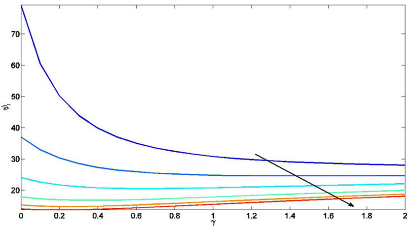
Figure 1. Effect of γ ∈ (0, 2] and α ∈ {0.25, 1, 2.5, 5, 10, 50} to the ultimate bound ψ₁ in equation (42), where the arrow indicate the direction α is increased.

3.3. Illustrative Numerical Example

We now present several numerical examples to illustrate the results given earlier in this section. For this purpose, consider a process composed of two decoupled systems with the dynamics given by equation (5), where

$\begin{array}{l}A=\left[\begin{array}{cccc}0& 1& 0& 0\\ -{\omega }_{\text{n}1}^2& -2{\omega }_{\text{n}1}{\mathrm{\xi }}_1& 0& 0\\ 0& 0& 0& 1\\ 0& 0& -{\omega }_{\text{n}2}^2& -2{\omega }_{\text{n}2}{\mathrm{\xi }}_2\end{array}\right],\hfill \end{array}$ (50)

$\begin{array}{l}B=\left[\begin{array}{cc}0& 0\\ {\omega }_{\text{n}1}^2& 0\\ 0& 0\\ 0& {\omega }_{\text{n}2}^2\end{array}\right]\hfill \end{array}$ (51)

ω_n1 = 1.2, ξ₁ = 0.9, ω_n2 = 0.5, and ξ₂ = 0.6. This process, for example, can represent a linearized vehicle model with the first and third states corresponding to the positions in the x and y directions, respectively, while the second and fourth states corresponding to the velocities in the x and y directions, respectively. The initial conditions are set to $x_0^{\text{T}}=\left[-3,0.5,2.5,0.25\right]$. In addition, we consider the input is given by

$w\left(t\right)=\left[\begin{array}{c}\hfill 2.5\text{\hspace{0.17em}sin}\left(t\right)\hfill \\ \hfill 4\text{\hspace{0.17em}cos}\left(1.2t\right)\hfill \end{array}\right].$ (52)

To maintain the readability of the paper, the values of L_i, σ_i, P_i in the following examples are put in Appendix B in Data Sheet in Supplementary Material.

Example 1. For the first example, we consider a sensor network with 12 nodes exchanging information over an undirected and connected graph topology, where there are 4 active nodes and 8 passive nodes as shown in Figure 2. Each node’s sensing capability is represented by equation (6) with the output matrices

$C_i=\left[\begin{array}{cccc}\hfill 1\hfill & \hfill 0\hfill & \hfill 0\hfill & \hfill 0\hfill \\ \hfill 0\hfill & \hfill 0\hfill & \hfill 1\hfill & \hfill 0\hfill \end{array}\right],$ (53)

for the odd index nodes and

$C_i=\left[\begin{array}{cccc}\hfill 0\hfill & \hfill 1\hfill & \hfill 0\hfill & \hfill 0\hfill \\ \hfill 0\hfill & \hfill 0\hfill & \hfill 0\hfill & \hfill 1\hfill \end{array}\right]$ (54)

for the even index nodes. In addition, all nodes are subject to zero initial conditions and we set J_i = K_i = diag([100; 100]), α = 50, and γ = 0.1. For the observer gain L_i, the odd index nodes are subject to [equation (A.6) in Supplementary Material] while the even index nodes are subject to [Equation (A.7) in Supplementary Material].

FIGURE 2

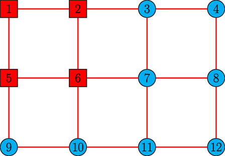
Figure 2. Communication graph of the sensor network in Example 1 with 4 active nodes and 8 passive nodes (lines denote communication links, squares denote active nodes, and circles denote passive nodes) Tran et al. (2017).

By solving the linear matrix inequality equation (9) for each node, σ_i and P_i > 0 are obtained as σ₁ = σ₅, σ₂ = σ₆, σ₃ = σ₄ = σ₇ = σ₈ = σ₉ = σ₁₀ = σ₁₁ = σ₁₂ where σ₁, σ₂, and σ₃ are subject to equations (A.8), (A.9), and (A.10) in Supplementary Material, respectively. In addition, P₁, P₂, and P₁₂ are subject to equations (A.11), (A.12), and (A.13) in Supplementary Material, respectively. Note that P₁ = P₅, P₂ = P₆, and P₃ = P₄ = P₇ = P₈ = P₉ = P₁₀ = P₁₁ = P₁₂. Under the proposed distributed estimation architecture equations (7) and (8), nodes are able to closely estimate the process states and inputs as shown in Figures 3 and 4, respectively. ▴

FIGURE 3

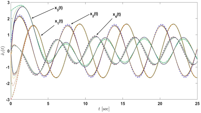
Figure 3. State estimates of the sensor network in Example 1 with 4 active nodes and 8 passive nodes under the proposed architecture equations (7) and (8) (the dash lines denote the states of the actual process and the solid lines denote the state estimates of nodes) Tran et al. (2017).

FIGURE 4

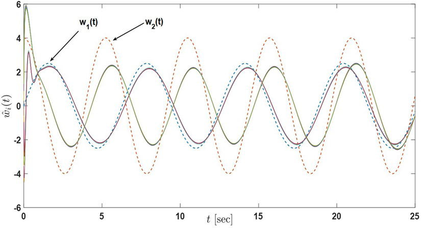
Figure 4. Input estimates of the sensor network in Example 1 with 4 active nodes and 8 passive nodes under the proposed architecture equations (7) and (8) (the dash lines denote the inputs of the actual process and the solid lines denote the input estimates of nodes) Tran et al. (2017).

Example 2. In this example, we increase the number of active nodes in the sensor network to 8 as depicted in Figure 5. The sensing capability of each agent is the same as in Example 1. Note that, because of the change in the number of active nodes, the design parameters are adjusted accordingly as σ₁ = σ₃ = σ₅ = σ₇, σ₂ = σ₄ = σ₆ = σ₈, σ₉ = σ₁₀ = σ₁₁ = σ₁₂ where σ₁, σ₂, and σ₉ are subjected to equations (A.14), (A.15), and (A.16) in Supplementary Material, respectively. In addition, P₁ = P₃ = P₅ = P₇, P₂ = P₄ = P₆ = P₈, P₉ = P₁₀ = P₁₁ = P₁₂, where P₁, P₂, and P₁₂ are the same as equations (A.11), (A.12), and (A.13) in Supplementary Material, respectively. Other parameters and gains are also kept the same. Figures 6 and 7 show the performance of the sensor network for the proposed distributed estimation architecture. In addition, in order to compare the performance of Example 1 and Example 2, the state and input error norms of both examples are plotted in Figures 8 and 9, respectively. The transient responses are captured in the figures approximately during the first 2 or 3 s, and it can be seen that Example 2 converges faster than Example 1 in state estimation, yet it encounters overshoot in input estimation. In addition, we can roughly approximate the average of both state and input error norms are reduced by a factor of 2 in Example 2 compared to Example 1. In general, Examples 1 and 2 show that the steady-state performance is improved by increasing the number of active nodes in the sensor network. ▴

FIGURE 5

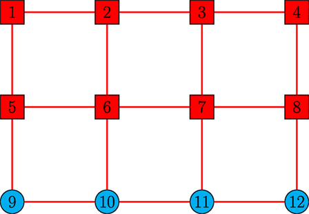
Figure 5. Communication graph of the sensor network in Examples 2 and 3 with 8 active nodes and 4 passive nodes (lines denote communication links, squares denote active nodes, and circles denote passive nodes) Tran et al. (2017).

FIGURE 6

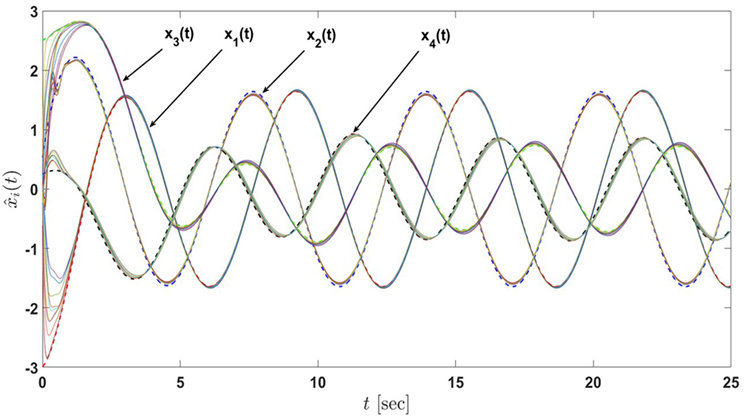
Figure 6. State estimates of the sensor network in Example 2 with 8 active nodes and 4 passive nodes under the proposed architecture equations (7) and (8) (the dash lines denote the states of the actual process and the solid lines denote the state estimates of nodes) Tran et al. (2017).

FIGURE 7

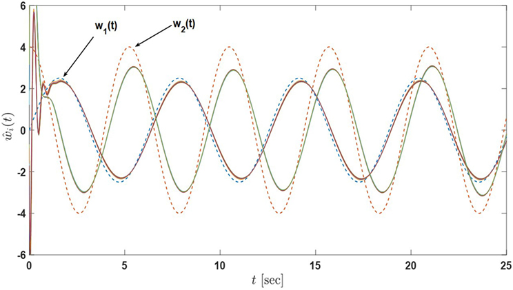
Figure 7. Input estimates of the sensor network in Example 2 with 8 active nodes and 4 passive nodes under the proposed architecture equations (7) and (8) (the dash lines denote the inputs of the actual process and the solid lines denote the input estimates of nodes) Tran et al. (2017).

FIGURE 8

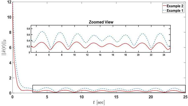
Figure 8. State error norms of the sensor networks in Example 1 and Example 2.

FIGURE 9

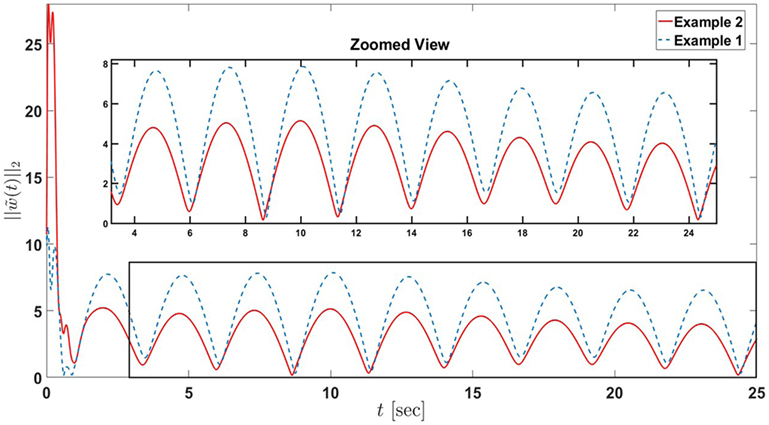
Figure 9. Input error norms of the sensor networks in Example 1 and Example 2.

Example 3. In this example, we consider a sensor network with 8 active nodes and 4 passive nodes as in Example 2 (Figure 5), but change the system output matrices for each node as follows

$\begin{array}{l}{C}_1=\left[\begin{array}{cccc}1& 0& 0& 0\\ 0& 0& 0& 0\end{array}\right],\hfill \end{array}$ (55)

$\begin{array}{l}{C}_2=\left[\begin{array}{cccc}0& 1& 0& 0\\ 0& 0& 0& 1\end{array}\right],\hfill \end{array}$ (56)

$C_3=\left[\begin{array}{cccc}\hfill 0\hfill & \hfill 0\hfill & \hfill 0\hfill & \hfill 0\hfill \\ \hfill 0\hfill & \hfill 0\hfill & \hfill 1\hfill & \hfill 0\hfill \end{array}\right],$ (57)

where C₁ = C₅ = C₉, C₂ = C₄ = C₆ = C₈ = C₁₀ = C₁₂, and C₃ = C₇ = C₁₁. Note that for the odd index nodes, the pair (A, C_i) is not observable. We also choose J_i = K_i = diag([100; 100]), α = 50, and γ = 0.1.

Here, the observer gain L_i is chosen such that L₁ = L₅ = L₉, L₂ = L₄ = L₆ = L₈ = L₁₀ = L₁₂, and L₃ = L₇ = L₁₁ where L₁, L₂, and L₃ are subject to equations (A.17), (A.18), and (A.19) in Supplementary Material, respectively. By solving the linear matrix inequality equation (9) for each node, σ_i and P_i > 0 are obtained as σ₁ = σ₅, σ₂ = σ₄ = σ₆ = σ₈, σ₃ = σ₇, and σ₉ = σ₁₀ = σ₁₁ = σ₁₂ where σ₁, σ₂, σ₃, and σ₉ are subject to equations (A.20), (A.21), (A.22), and (A.23) in Supplementary Material, respectively. In addition, P₁ = P₅, P₂ = P₄ = P₆ = P₈, P₃ = P₇, and P₉ = P₁₀ = P₁₁ = P₁₂ where P₁, P₂, P₃, and P₁₂ are subject to equations (A.24), (A.12), (A.25), and (A.13) in Supplementary Material, respectively. Figures 10 and 11 show that under the proposed distributed estimation architecture, nodes are able to closely estimate the process states and inputs, although some active nodes are not able to fully observe the process. ▴

FIGURE 10

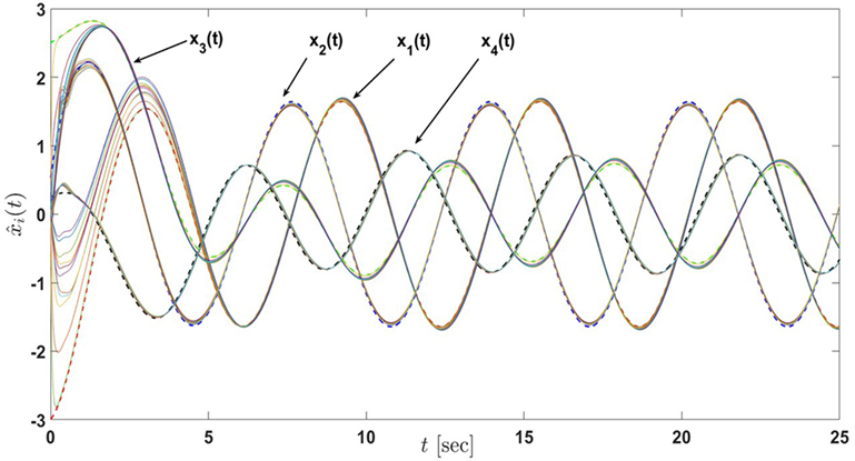
Figure 10. State estimates of the sensor network in Example 3 with 12 active nodes under the proposed architecture equations (7) and (8) (the dash lines denote the states of the actual process and the solid lines denote the state estimates of nodes) Tran et al. (2017).

FIGURE 11

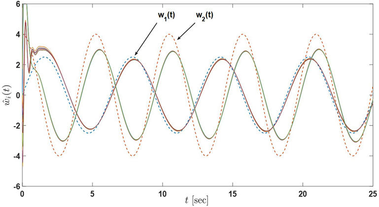
Figure 11. Input estimates of the sensor network in Example 3 with 12 active nodes under the proposed architecture equations (7) and (8) (the dash lines denote the inputs of the actual process and the solid lines denote the input estimates of nodes) Tran et al. (2017).

4. Distributed Input and State Estimation for Active-Passive Sensor Networks with Varying Node Roles

We now generalize the results of the previous section to the case when the active and passive role of each sensor node is varying over time. For this purpose, once again, we consider a process given by equations (5). In addition, if a node in the sensor network is active for some time instant, then it is subject to the observations of the process given by equation (6) on that time instant, otherwise it is a passive node and has no observation. Note that a node is assumed to be smoothly changed back and forth between active and passive mode (i.e., g_i(t) is a smooth function on the interval [0, 1]). The proposed algorithm is discussed in Section 4.1, followed by the stability analysis (Section 4.2), and a numerical example is presented to illustrate the efficacy of the methods (Section 4.3).

4.1. Proposed Distributed Estimation Architecture

For node i, i = 1, …, N, consider the distributed estimation algorithm given by

$\begin{array}{l}{\dot{\widehat{x}}}_i\left(t\right)=\left(A-\gamma P_i^{-1}\right){\widehat{x}}_i\left(t\right)+B{\widehat{w}}_i\left(t\right)+g_i\left(t\right)L_i\left(y_i\left(t\right)-C_i{\widehat{x}}_i\left(t\right)\right)-\hfill \\ \mathrm{\alpha }{P}_i^{-1}{\displaystyle \sum _{i\sim j}}\left({\widehat{x}}_i\left(t\right)-{\widehat{x}}_j\left(t\right)\right),{\widehat{x}}_i\left(0\right)={\widehat{x}}_{i0},\end{array}$ (58)

$\begin{array}{l}{\dot{\widehat{w}}}_i\left(t\right)=g_i\left(t\right)J_i\left(y_i\left(t\right)-C_i{\widehat{x}}_i\left(t\right)\right)-\left({\sigma }_i{K}_i+\gamma {\text{I}}_p\right){\widehat{w}}_i\left(t\right)\hfill \\ -\mathrm{\alpha }{\displaystyle \sum _{i\sim j}}\left({\widehat{w}}_i\left(t\right)-{\widehat{w}}_j\left(t\right)\right),{\widehat{w}}_i\left(0\right)={\widehat{w}}_{i0},\end{array}$ (59)

where ${\widehat{x}}_i\left(t\right)\in {\mathbb{R}}^n$ is a local state estimate of x(t) for node i, ${\widehat{w}}_i\in {\mathbb{R}}^p$ is a local input estimate of w(t) for node i, $L_i\in {\mathbb{R}}^{n\times m}$, $J_i\in {\mathbb{R}}^{p\times m}$, and $K_i\in {\mathbb{S}}_{+}^{p\times p}$ are design matrices of node i, and α, γ, and ${\sigma }_i\in \mathbb{R}$ are positive design coefficients for node i. Note that the parameter g_i(t) in this section is time-varying and g_i(t) ∈ [0, 1]. In addition, P_i > 0 is the consensus gain satisfying the two linear matrix inequalities given by

$\begin{array}{l}{R}_{i1}\triangleq \left[\begin{array}{cc}{A}^{\text{T}}{P}_i+P_{i}A& -P_{i}B\\ -B^{\text{T}}{P}_i& -2{\sigma }_i{K}_i\end{array}\right]\le 0,\hfill \end{array}$ (60)

$\begin{array}{l}{R}_{i2}\triangleq \left[\begin{array}{cc}{\left(A-L_i{C}_i\right)}^{\text{T}}{P}_i+P_i\left(A-L_i{C}_i\right)& -P_{i}B+C_i^{\text{T}}{J}_i^{\text{T}}\\ -B^{\text{T}}{P}_i+J_i{C}_i& -2{\sigma }_i{K}_i\end{array}\right]\le 0,i=1,\dots ,N.\hfill \end{array}$ (61)

4.2. Stability Analysis

Let ${\tilde{x}}_i\left(t\right)\triangleq x\left(t\right)-{\widehat{x}}_i\left(t\right)$ and ${\tilde{w}}_i\left(t\right)\triangleq {\widehat{w}}_i\left(t\right)-w\left(t\right)$. Then, similar to equations (11) and (12), one can write

$\begin{array}{l}{\dot{\tilde{x}}}_i\left(t\right)={\overline{A}}_i\left(t\right){\tilde{x}}_i\left(t\right)-B{\tilde{w}}_i\left(t\right)-\mathrm{\alpha }{P}_i^{-1}{\displaystyle \sum _{i\sim j}}\left({\tilde{x}}_i\left(t\right)-{\tilde{x}}_j\left(t\right)\right)-\mathrm{\gamma }{P}_i^{-1}\left({\tilde{x}}_i\left(t\right)-x\left(t\right)\right),{\tilde{x}}_i\left(0\right)={\tilde{x}}_{i0},\hfill \end{array}$ (62)

$\begin{array}{l}{\dot{\tilde{w}}}_i\left(t\right)=g_i\left(t\right)J_i{C}_i{\tilde{x}}_i\left(t\right)-{\sigma }_i{K}_i\left({\tilde{w}}_i\left(t\right)+w\left(t\right)\right)-\mathrm{\alpha }{\displaystyle \sum _{i\sim j}}({\tilde{w}}_i\left(t\right)\hfill \\ -{\tilde{w}}_j\left(t\right))-\mathrm{\gamma }\left({\tilde{w}}_i\left(t\right)+w\left(t\right)\right)-\dot{w}\left(t\right),{\tilde{w}}_i\left(0\right)={\tilde{w}}_{i0},\end{array}$ (63)

where

${\overline{A}}_i\left(t\right)\triangleq A-g_i\left(t\right)L_i{C}_i.$ (64)

Therefore, similar to Section 3.2, the compact form of the error dynamics are given by

$\begin{array}{l}\dot{\tilde{x}}\left(t\right)=\overline{A}\left(t\right)\tilde{x}\left(t\right)-\left({\text{I}}_N\otimes B\right)\tilde{w}\left(t\right)-P^{-1}\left(F\otimes {\text{I}}_n\right)\tilde{x}\left(t\right)+\mathrm{\gamma }{P}^{-1}\left({\mathbf{\text{1}}}_N\otimes {\text{I}}_n\right)x\left(t\right),\hfill \end{array}$ (65)

$\begin{array}{l}\dot{\tilde{w}}\left(t\right)=M\left(t\right)\tilde{x}\left(t\right)-\overline{K}\left(\tilde{w}\left(t\right)+\left({\mathbf{\text{1}}}_N\otimes {\text{I}}_p\right)w\left(t\right)\right)-\left(F\otimes {\text{I}}_p\right)\tilde{w}\left(t\right)\hfill \\ -\mathrm{\gamma }\left({\mathbf{\text{1}}}_N\otimes {\text{I}}_p\right)w\left(t\right)-\left({\mathbf{\text{1}}}_N\otimes {\text{I}}_p\right)\dot{w}\left(t\right),\end{array}$ (66)

where

$\begin{array}{l}\overline{A}\left(t\right)\triangleq \text{\hspace{0.17em}diag\hspace{0.17em}}\left(\left[{\overline{A}}_1\left(t\right),{\overline{A}}_2\left(t\right),\dots ,{\overline{A}}_N\left(t\right)\right]\right),\hfill \end{array}$ (67)

$\begin{array}{l}M\left(t\right)\triangleq \text{\hspace{0.17em}diag\hspace{0.17em}}\left(\left[g_1\left(t\right)J_1{C}_1,g_2\left(t\right)J_2{C}_2,\dots ,g_N\left(t\right)J_N{C}_N\right]\right),\hfill \end{array}$ (68)

and $\overline{K}$, F, and P are the same as equations (21), (22), and (23), respectively.

Theorem 2. Consider the process given by equation (5) and the distributed input and state estimation architecture given by equations (58) and (59). Assume equations (60) and (61) hold and nodes exchange information using local that measurements subject to an undirected and connected graph 𝒢. Then, the error dynamics given by equations (65) and (66) are uniformly ultimately bounded.

Proof. Consider the Lyapunov function candidate given by equation (24). Following the steps from the proof of Theorem 1, differentiating equation (24) along the trajectories of equations (65) and (66) yields

$\dot{V}\left(\cdot \right)=z^{\text{T}}\left(t\right)R_A\left(t\right)z\left(t\right)+z^{\text{T}}\left(t\right)R_{B}z\left(t\right)+2z^{\text{T}}\left(t\right)\varphi ,$ (69)

where z(t), R_B, and ϕ are defined in equations (26), (28), and (30), respectively. In addition,

$R_A\left(t\right)\triangleq \left[\begin{array}{cc}\hfill \overline{A}{\left(t\right)}^{\text{T}}P+P\overline{A}\left(t\right)\hfill & \hfill -P\left({\text{I}}_N\otimes B\right)+M^{\text{T}}\left(t\right)\hfill \\ \hfill -\left({\text{I}}_N\otimes B^{\text{T}}\right)P+M\left(t\right)\hfill & \hfill -2\overline{K}\hfill \end{array}\right].$ (70)

Note that for this varying case of active and passive node roles, R_i in equation (9) becomes

$\begin{array}{l}{R}_i\left(t\right)=\left[\begin{array}{cc}{\left(A-g_i\left(t\right)L_i{C}_i\right)}^{\text{T}}{P}_i+P_i\left(A-g_i\left(t\right)L_i{C}_i\right)& -P_{i}B+g_i\left(t\right)C_i^{\text{T}}{J}_i^{\text{T}}\\ -B^{\text{T}}{P}_i+g_i\left(t\right)J_i{C}_i& -2{\sigma }_i{K}_i\end{array}\right]\hfill \\ =\left[\begin{array}{cc}{A}^{\text{T}}{P}_i+P_{i}A& -P_{i}B\\ -B^{\text{T}}{P}_i& -2{\sigma }_i{K}_i\end{array}\right]+g_i\left(t\right)\left[\begin{array}{cc}{\left(-L_i{C}_i\right)}^{\text{T}}{P}_i+P_i\left(-L_i{C}_i\right)& C_i^{\text{T}}{J}_i^{\text{T}}\\ J_i{C}_i& 0\end{array}\right].\end{array}$ (71)

Since g_i(t) ∈ [0, 1], R_i1 in equation (60) and R_i2 in equation (61) corresponds to g_i(t) = 0 and g_i(t) = 1 in equation (71), respectively. Therefore, R_i1 and R_i2 are the vertices of the polytope. By Lemma 3, when the linear matrix inequalities equations (60) and (61) hold, R_i(t) ≤ 0 for all g_i(t) ∈ [0, 1]. Consequently, using the same argument as in the proof of Theorem 1, we have R_A(t) ≤ 0. Hence, equation (69) becomes

$\begin{array}{ll}\dot{V}\left(\cdot \right)\hfill & =z^{\text{T}}\left(t\right)R_A\left(t\right)z\left(t\right)+z^{\text{T}}\left(t\right)R_{B}z\left(t\right)+2z^{\text{T}}\left(t\right)\varphi \\ \hfill & \le {\mathrm{\lambda }}_{\text{max}}\left(R_B\right)||z\left(t\right){||}_2^2+2||z\left(t\right){||}_2\overline{\varphi }\\ \hfill & \le \left(1-\theta \right){\mathrm{\lambda }}_{\text{max}}\left(R_B\right)||z\left(t\right){||}_2^2+\theta {\mathrm{\lambda }}_{\text{max}}\left(R_B\right)||z\left(t\right){||}_2^2+2||z\left(t\right){||}_2\overline{\varphi },\end{array}$ (72)

with λ_max(R_B) < 0 and θ ∈ (0, 1). Letting ${\mu }_2\triangleq \frac{-2\overline{\varphi }}{\theta {\mathrm{\lambda }}_{\text{max}}\left(R_B\right)}>0$ and ${\mathrm{\Omega }}_2\triangleq \left\{z\left(t\right):||z\left(t\right){||}_2\le {\mu }_2\right\}$, it follows that $\dot{V}\left(\cdot \right)\le \left(1-\theta \right){\mathrm{\lambda }}_{\text{max}}\left(R_B\right)||z\left(t\right){||}_2^2<0$ outside the compact set Ω₂ and, hence, the error dynamics given by equations (62) and (63) are uniformly ultimately bounded from Theorem 4.18 in Khalil (2002). ■

Corollary 2. Consider the process given by equation (5) and the distributed input and state estimation architecture given by equations (58) and (59). Assume that equations (60) and (61) hold and nodes exchange information using local measurements subject to an undirected and connected graph 𝒢. Then, for all $z\left(0\right)\in {\mathbb{R}}^{N\left(n+p\right)}$, there exists T = T(z(0), μ₂) ≥ 0 such that

$\begin{array}{l}||\tilde{x}\left(t\right){||}_2\le {\mathrm{\xi }}_2\triangleq \sqrt{\frac{{\mathrm{\lambda }}_{\text{max}}\left(\overline{P}\right)}{{\mathrm{\lambda }}_{\text{min}}\left(\overline{P}\right)}}\max \{||z\left(0\right){||}_2\times e^{\left(\left(1-\theta \right){\mathrm{\lambda }}_{\text{max}}\left(R_B\right)∕2{\mathrm{\lambda }}_{\text{max}}\left(\overline{P}\right)\right)t},{\mu }_2\},\forall t\ge 0,\hfill \end{array}$ (73)

$\begin{array}{ll}||\tilde{w}\left(t\right){||}_2\hfill & \le {\mathrm{\xi }}_2,\forall t\ge 0,\end{array}$ (74)

where

$\overline{P}=\left[\begin{array}{cc}\hfill P\hfill & \hfill 0\hfill \\ \hfill 0\hfill & \hfill {\mathrm{I}}_{\mathit{Np}}\hfill \end{array}\right],$ (75)

and

$||\tilde{x}\left(t\right){||}_2\le {\psi }_2\triangleq \sqrt{\frac{{\mathrm{\lambda }}_{\text{max}}\left(\overline{P}\right)}{{\mathrm{\lambda }}_{\text{min}}\left(P\right)}}{\mu }_2,t\ge T,$ (76)

$||\tilde{w}\left(t\right){||}_2\le {\mathrm{\zeta }}_2\triangleq \sqrt{{\mathrm{\lambda }}_{\text{max}}\left(\overline{P}\right)}{\mu }_2,t\ge T.$ (77)

Proof. Same theoretical steps follow from the proof of Corollary 1 and, hence, the proof is omitted here. ■

4.3. Illustrative Numerical Example

In this section, we present numerical examples to illustrate the results discussed in Sections 4.1 and 4.2. For this purpose, we consider a process as the vehicle model depicted in Section 3.3 with the dynamics given by equation (5), where A and B are defined in equations (50) and (51), respectively. To maintain the readability of the paper, the values of L_i, σ_i, P_i in the following examples are put in Appendix B in Data Sheet in Supplementary Material.

Example 4. For this example, the initial conditions of the process are set to $x_0^{\text{T}}=\left[-3,0.5,2.5,0.25\right]$. In addition, we consider the input is given by

$w\left(t\right)=\left[\begin{array}{c}\hfill 2.5\text{\hspace{0.17em}sin}\left(t\right)\hfill \\ \hfill 3.5\text{\hspace{0.17em}cos}\left(1.2t\right)\hfill \end{array}\right].$ (78)

We now consider an active-passive sensor network with 12 nodes exchanging information over an undirected and connected graph topology as presented in Figure 12, where the active and passive roles of each node is varying overtime. Specifically, the sensors are distributed over an area, and each sensor position is shown in Figure 12. Suppose that each sensor sensing range is a circle with the radius r = 3. Recall that the first and third states of the process (or the vehicle) correspond to the positions in the x-axis and y-axis directions, respectively. If the vehicle’s position is within a sensor sensing range, then that sensor becomes smoothly active. On the other hand, if the vehicle’s position is out of the sensor sensing range, then it becomes smoothly passive. Note that, for the transition of g_i(t), we use the function $g_i\left(t\right)=e^{-\mathrm{\beta }t}$ when node i is switching from 1 to 0, and $g_i\left(t\right)=1-e^{-\mathrm{\beta }t}$ when node i is switching from 0 to 1, where β is a positive constant. We adapt this transition from Figure 2D of Zavlanos et al. (2011). The network has two types of sensors, and each node’s sensing capability is represented by equation (6) with the output matrices

$C_i=\left[\begin{array}{cccc}\hfill 1\hfill & \hfill 0\hfill & \hfill 0\hfill & \hfill 0\hfill \\ \hfill 0\hfill & \hfill 0\hfill & \hfill 1\hfill & \hfill 0\hfill \end{array}\right],$ (79)

for the odd index nodes and

$C_i=\left[\begin{array}{cccc}\hfill 0\hfill & \hfill 1\hfill & \hfill 0\hfill & \hfill 0\hfill \\ \hfill 0\hfill & \hfill 0\hfill & \hfill 0\hfill & \hfill 1\hfill \end{array}\right]$ (80)

for the even index nodes. Note that the pair (A, C_i) is observable for all i = 1, …, 12 in this example and, therefore, the collective observability assumption is satisfied. All nodes are subjected to zero initial conditions and we set J_i = K_i = diag([100; 100]), α = 50, and γ = 0.1. For the observer gain L_i, the odd index nodes are subject to [equation (A.26) in Supplementary Material] while the even index nodes are subject to [equation (A.27) in Supplementary Material].

FIGURE 12

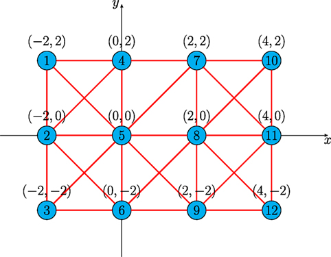
Figure 12. Communication graph of the active-passive sensor network in Example 4 with 12 nodes (lines denote communication links, circles denote nodes).

By solving the linear matrix inequalities equations (60) and (61) simultaneously for each node, σ_i and P_i > 0 are obtained as σ₁ = σ₃ = σ₅ = σ₇ = σ₉ = σ₁₁ and σ₂ = σ₄ = σ₆ = σ₈ = σ₁₀ = σ₁₂ where σ₁ and σ₂ are subject to equations (A.28) and (A.29) in Supplementary Material, respectively. In addition, P₁ and P₂ are subject to equations (A.30) and (A.31) in Supplementary Material, respectively. Note that P₁ = P₃ = P₅ = P₇ = P₉ = P₁₁ and P₂ = P₄ = P₆ = P₈ = P₁₀ = P₁₂.

Under the proposed distributed estimation architecture equations (58) and (59), nodes are able to closely estimate the process states as shown in Figure 13. Specifically, Figure 14 illustrates that the sensor network is able to estimate the trajectory of the vehicle (the first and third states of the process), while the input estimated in Figure 15 is not as good as the case for fixed node roles presented in Section 3.3, this can be explained by the conservatism of the solution of the linear matrix inequalities equations (60) and (61). That is, if we had the flexibility to make the σ_i values small such that σ₁ = σ₃ = σ₅ = σ₇ = σ₉ = σ₁₁ = 0.001 and σ₂ = σ₄ = σ₆ = σ₈ = σ₁₀ = σ₁₂ = 0.001, while keeping P_i and other parameters the same, the performance of the input and state estimate would become better as shown in Figures 16 and 17, respectively. However, with these small values of σ_i, the linear matrix inequalities equations (60) and (61) are no longer satisfied. Numerical methods to reduce such conservatism in linear matrix inequality computations for equations (60) and (61) and/or relax the linear matrix inequality condition will be investigated as a future research.

FIGURE 13

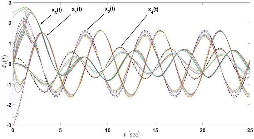
Figure 13. State estimates of the active-passive sensor network in Example 4 with 12 nodes under the proposed architecture equations (58) and (59) and satisfying the linear matrix inequalities equations (60) and (61) (the dash lines denote the states of the actual process and the solid lines denote the state estimates of nodes).

FIGURE 14

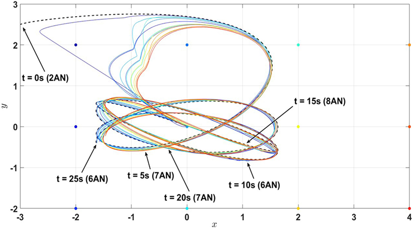
Figure 14. Position estimates (first and third states of the process) of the active-passive sensor network in Example 4 with 12 nodes under the proposed architecture equations (58) and (59) and satisfying the linear matrix inequalities equations (60) and (61) (the dash line denote the trajectory of the actual process (i.e., the combination of the first and third states) and the solid lines denote the state estimates of nodes). Here, AN stands for the active nodes.

FIGURE 15

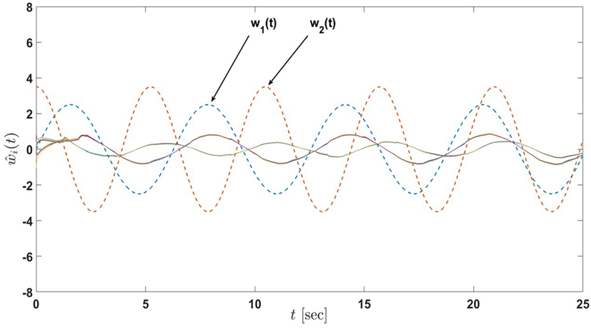
Figure 15. Input estimates of the active-passive sensor network in Example 4 with 12 nodes under the proposed architecture equations (58) and (59) and satisfying the linear matrix inequalities equations (60) and (61) (the dash lines denote the inputs of the actual process and the solid lines denote the input estimates of nodes).

FIGURE 16

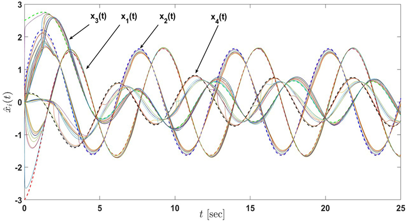
Figure 16. State estimates of the active-passive sensor network in Example 4 with 12 nodes under the proposed architecture equations (58) and (59) with the decrease in σ_i, i = 1, …, 12 (the dash lines denote the states of the actual process and the solid lines denote the state estimates of nodes).

FIGURE 17

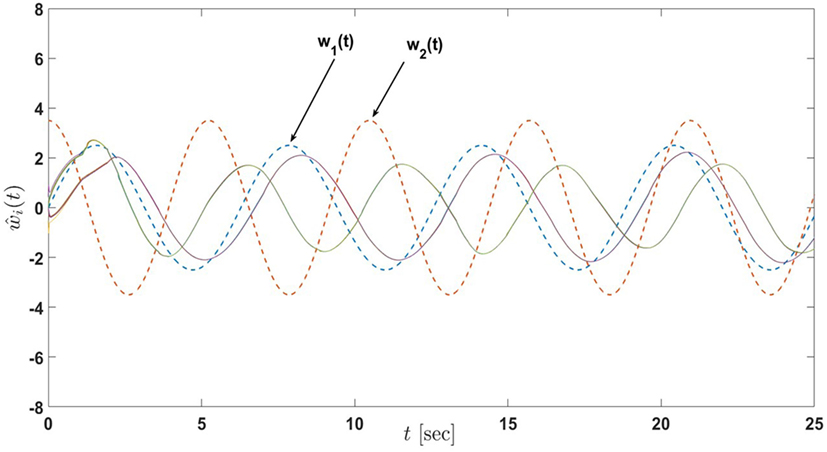
Figure 17. Input estimates of the active-passive sensor network in Example 4 with 12 nodes under the proposed architecture equations (58) and (59) with the decrease in σ_i, i = 1, …, 12 (the dash lines denote the inputs of the actual process and the solid lines denote the input estimates of nodes).

Example 5. For this example, the initial conditions of the process are set to $x_0^{\text{T}}$ = [−2, 0.5, 2.5, 0.25]. In addition, we consider the input is given by

$w\left(t\right)=\left[\begin{array}{c}\hfill 1.5\text{\hspace{0.17em}sin}\left(0.5t\right)\hfill \\ \hfill 3\text{\hspace{0.17em}cos}\left(0.6t\right)\hfill \end{array}\right].$ (81)

We now consider an active-passive sensor network with 13 nodes labeled, respectively, as 1a, 1b, 2a, 2b, 3a, 3b, 4a, 4b, 5, 6, 7, 8, and 9, exchanging information over an undirected and connected graph topology as presented in Figure 18, where the active and passive role of each node is varying overtime. Specifically, the sensors are distributed over an area with each pair of nodes Xa and Xb (where X = 1, 2, 3, 4 and denoted as diamond in Figure 18) is grouped at the same location such that when Xa is active (or passive), so is Xb and vice versa; Xa and Xb are neighbors of each other and have the same set of neighbors.

FIGURE 18

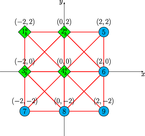
Figure 18. Communication graph of the active-passive sensor network in Example 5 with 13 nodes (lines denote communication links, circles denote normal nodes, and diamond denotes overlapped nodes).

Suppose that each sensor sensing range is a circle with the radius r = 3.5. Note that, for the transition of g_i(t), we use the same functions as Example 4. The network has six types of sensors, and each node’s sensing capability is represented by equation (6) with the output matrices

$C_{1a}=\left[\begin{array}{cccc}\hfill 1\hfill & \hfill 0\hfill & \hfill 0\hfill & \hfill 0\hfill \\ \hfill 0\hfill & \hfill 0\hfill & \hfill 0\hfill & \hfill 0\hfill \end{array}\right],$ (82)

$\begin{array}{l}{C}_{1b}=\left[\begin{array}{cccc}0& 0& 0& 0\\ 0& 0& 1& 0\end{array}\right],\hfill \end{array}$ (83)

$\begin{array}{l}{C}_{2b}=\left[\begin{array}{cccc}0& 0& 0& 0\\ 0& 0& 0& 1\end{array}\right],\hfill \end{array}$ (84)

$\begin{array}{l}{C}_{3a}=\left[\begin{array}{cccc}0& 1& 0& 0\\ 0& 0& 0& 0\end{array}\right],\hfill \end{array}$ (85)

$\begin{array}{l}{C}_5=\left[\begin{array}{cccc}1& 0& 0& 0\\ 0& 0& 1& 0\end{array}\right],\hfill \end{array}$ (86)

$\begin{array}{l}{C}_6=\left[\begin{array}{cccc}0& 1& 0& 0\\ 0& 0& 0& 1\end{array}\right].\hfill \end{array}$ (87)

In addition, C_1a = C_2a, C_1b = C_3b, C_2b = C_4b, C_3a = C_4a, C₅ = C₇ = C₉, and C₆ = C₈. Note that the pairs (A, C_Xa) and (A, C_Xb) where X = 1, 2, 3, 4 are not observable, but with the setup of the problem (nodes Xa and Xb are either active or both passive simultaneously), the collective observability condition is guaranteed. All nodes are subjected to zero initial conditions and we set J_i = K_i = diag([25; 25]), α = 75, and γ = 0.01. The observer gains L_i are set to L_1a = L_2a, L_1b = L_3b, L_2b = L_4b, L_3a = L_4a, L₅ = L₇ = L₉, and L₆ = L₈ where the gains L_1a, L_1b, L_2b, L_3a, L₅, and L₆ are subject to equations (A.32), (A.33), (A.34), (A.35), (A.36), and (A.37) in Supplementary Material, respectively.

By solving the linear matrix inequalities equations (60) and (61) simultaneously for each node, σ_i and P_i > 0 are obtained as σ_1a = σ_2a, σ_1b = σ_3b, σ_2b = σ_4b, σ_3a = σ_4a, σ₅ = σ₇ = σ₉ and σ₆ = σ₈ where σ_1a, σ_1b, σ_2b, σ_3a, σ₅ and σ₆ are subject to equations (A.38), (A.39), (A.40), (A.41), (A.42), and (A.43) in Supplementary Material, respectively. In addition, P_1a, P_1b, P_2b, P_3a, P₅, and P₆ are subject to equations (A.44), (A.45), (A.46), (A.47), (A.48), and (A.49) in Supplementary Material, respectively. Note that P_1a = P_2a, P_1b = P_3b, P_2b = P_4b, P_3a = P_4a, P₅ = P₇ = P₉, and P₆ = P₈.

Under the proposed distributed estimation architecture equations (58) and (59), nodes are able to closely estimate the process states as shown in Figure 19. Specifically, Figure 20 illustrates that the sensor network is able to estimate the trajectory of the vehicle (the first and third states of the process), while the input estimated in Figure 21 is still not as good as the case for fixed node roles presented in Section 3.3. Again, this can be explained by the conservatism of the solution of the linear matrix inequalities equations (60) and (61). If we had the flexibility to reduce σ_i to small values, for example, σ_i = 0.001, while keeping other parameters the same, the performance of the input and state estimate would become much better as shown in Figures 22 and 23, respectively. Note that with the choice of σ_i = 0.001 for this example, the linear matrix inequalities equations (60) and (61) are no longer satisfied. Once again, numerical methods to reduce such conservatism in linear matrix inequality computations for equations (60) and (61) and/or relax the linear matrix inequality condition will be investigated as a future research.

FIGURE 19

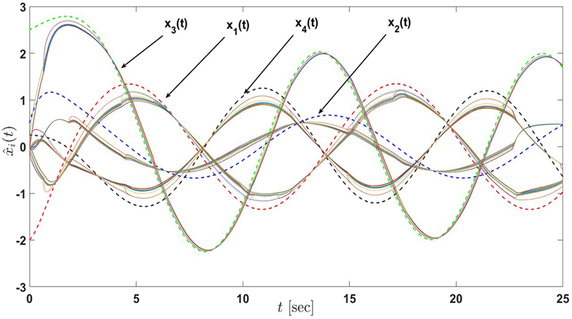
Figure 19. State estimates of the active-passive sensor network in Example 5 with 13 nodes under the proposed architecture equations (58) and (59) and satisfying the linear matrix inequalities equations (60) and (61) (the dash lines denote the states of the actual process and the solid lines denote the state estimates of nodes).

FIGURE 20

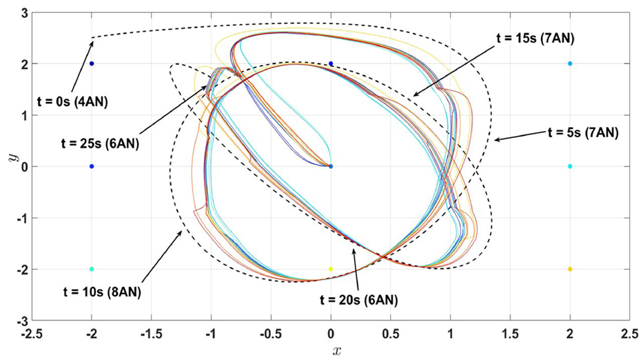
Figure 20. Position estimates (first and third states of the process) of the active-passive sensor network in Example 5 with 13 nodes under the proposed architecture equations (58) and (59) and satisfying the linear matrix inequalities equations (60) and (61) (the dash line denote the trajectory of the actual process (i.e., the combination of the first and third states) and the solid lines denote the state estimates of nodes). Here, AN stands for the active nodes.

FIGURE 21

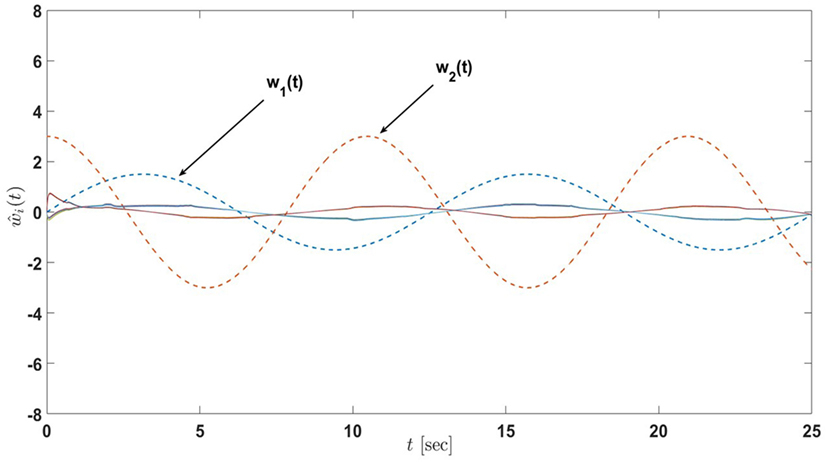
Figure 21. Input estimates of the active-passive sensor network in Example 5 with 13 nodes under the proposed architecture equations (58) and (59) and satisfying the linear matrix inequalities equations (60) and (61) (the dash lines denote the inputs of the actual process and the solid lines denote the input estimates of nodes).

FIGURE 22

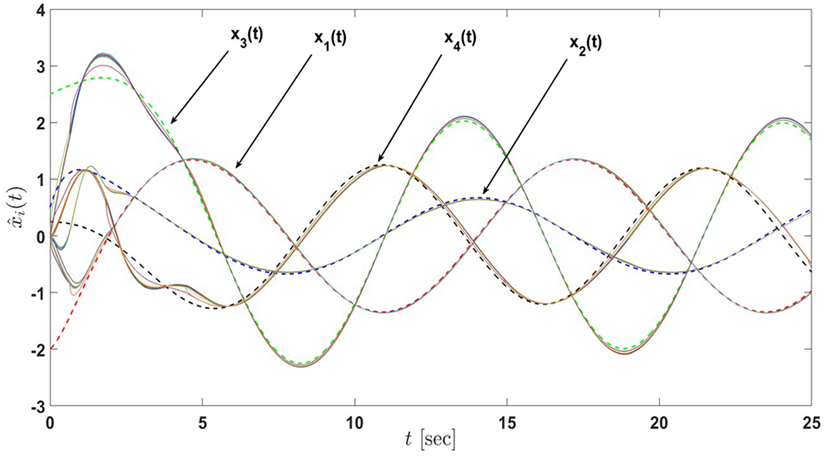
Figure 22. State estimates of the active-passive sensor network in Example 5 with 13 nodes under the proposed architecture equations (58) and (59) with the decrease in σ_i, i = 1, …, 12 (the dash lines denote the states of the actual process and the solid lines denote the state estimates of nodes).

FIGURE 23

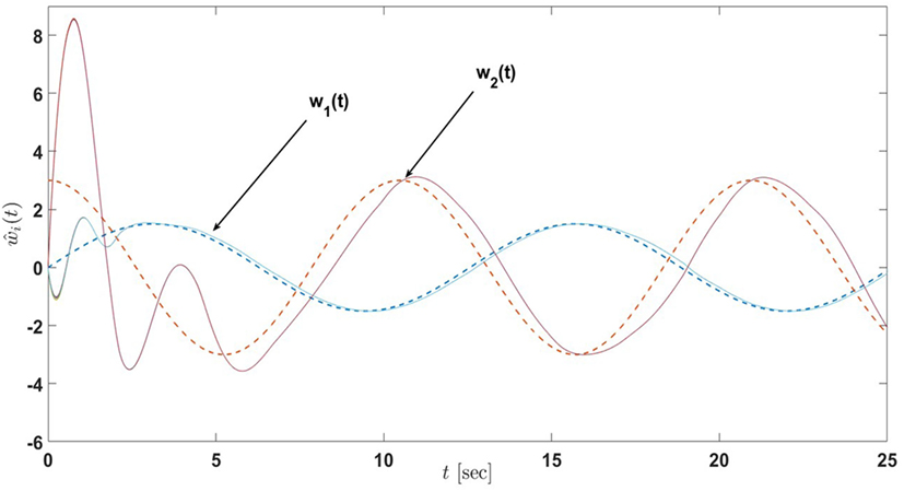
Figure 23. Input estimates of the active-passive sensor network in Example 5 with 13 nodes under the proposed architecture equations (58) and (59) with the decrease in σ_i, i = 1, …, 12 (the dash lines denote the inputs of the actual process and the solid lines denote the input estimates of nodes).

5. Conclusion

A distributed input and state estimation architecture was investigated for heterogeneous sensor networks having nodes with both fixed and varying active and passive information processing roles and non-identical sensor modalities. It was shown that the proposed framework utilizes local information not only during the execution of the proposed estimation algorithm but also in its design; that is, global uniform ultimate boundedness of error dynamics is guaranteed once each node satisfies given local stability conditions independent from the graph topology and neighboring information of these nodes. Several numerical examples illustrated the efficacy of the proposed architectures. Future research will include applications of the proposed framework to dynamic data-driven sensor network scenarios to guide and control autonomous vehicles and we will also consider extensions to time-varying graph topologies. It should be also mentioned especially for the results in Section 4 that structural sensor network construction to always guarantee collective observability is another interesting future research direction that will be considered by the authors.

Author Contributions

DT and TY were the technical leads of this paper, where they developed the proposed distributed estimation architecture. Specifically, DT played a key role in establishing the technical proofs of the proposed architecture, including how the analysis can be performed in a local fashion and TY played a key role in fleshing out the technical tools and methods needed to accomplish the documented research. SS and SJ assisted DT and TY in all technical and numerical aspects of this paper. In addition to theory development in terms of establishing the technical proofs, DT also numerically illustrated the proposed distributed estimation architecture.

Conflict of Interest Statement

The authors declare that the research was conducted in the absence of any commercial or financial relationships that could be construed as a potential conflict of interest.

The reviewer, OA, and handling editor declared their shared affiliation, and the handling editor states that the process nevertheless met the standards of a fair and objective review.

Acknowledgments

The authors wish to thank the reviewers for their constructive suggestions.

Funding

This research has been supported by the Dynamic Data-Driven Applications Systems Program of the Air Force Office of Scientific Research [grant number FA9550-17-1-0303].

Supplementary Material

The Supplementary Material for this article can be found online at https://www.frontiersin.org/article/10.3389/frobt.2017.00030/full#supplementary-material.

References

Akhenak, A., Chadli, M., Maquin, D., and Ragot, J. (2004). “State estimation of uncertain multiple model with unknown inputs,” in IEEE Conference on Decision and Control, Nassau.

Google Scholar

Bai, H., Freeman, R. A., and Lynch, K. M. (2010). “Robust dynamic average consensus of time-varying inputs,” in Conference on Decision and Control, Atlanta, 3104–3109.

Google Scholar

Bernstein, D. S. (2009). Matrix Mathematics: Theory, Facts, and Formulas. Princeton, NJ: Princeton University Press.

Google Scholar

Bowong, S., and Tewa, J. J. (2008). Unknown inputs adaptive observer for a class of chaotic systems with uncertainties. Math. Comput. Model. 48, 1826–1839. doi: 10.1016/j.mcm.2007.12.028

CrossRef Full Text | Google Scholar

Boyd, S., and Vandenberghe, L. (2004). Convex Optimization. Cambridge: Cambridge University Press.

Google Scholar

Boyd, S. P., El Ghaoui, L., Feron, E., and Balakrishnan, V. (1994). Linear Matrix Inequalities in System and Control Theory, Vol. 15. SIAM.

Google Scholar

Casbeer, D. W., Cao, Y., Garcia, E., and Milutinović, D. (2015). “Average bridge consensus: dealing with active-passive sensors,” in ASME Dynamic Systems and Control Conference, Columbus.

Google Scholar

Chen, F., Cao, Y., and Ren, W. (2012). Distributed average tracking of multiple time-varying reference signals with bounded derivatives. IEEE Trans. Automat. Contr. 57, 3169–3174. doi:10.1109/TAC.2012.2199176

CrossRef Full Text | Google Scholar

Chen, W., and Chowdhury, F. N. (2007). Simultaneous identification of time-varying parameters and estimation of system states using iterative learning observers. Int. J. Syst. Sci. 38, 39–45. doi:10.1080/00207720601042934

CrossRef Full Text | Google Scholar

Corless, M., and Tu, J. (1998). State and input estimation for a class of uncertain systems. Automatica 34, 757–764. doi:10.1016/S0005-1098(98)00013-2

CrossRef Full Text | Google Scholar

Cunningham, A., Indelman, V., and Dellaert, F. (2013). “DDF-SAM 2.0: consistent distributed smoothing and mapping,” in 2013 IEEE International Conference on Robotics and Automation (Karlsruhe: IEEE), 5220–5227.

Google Scholar

Demetriou, M. A. (2009). Natural consensus filters for second order infinite dimensional systems. Syst. Control Lett. 58, 826–833. doi:10.1016/j.sysconle.2009.10.001

CrossRef Full Text | Google Scholar

Freeman, R. A., Yang, P., and Lynch, K. M. (2006). “Stability and convergence properties of dynamic average consensus estimators,” in IEEE Conference on Decision and Control, San Diego, CA.

Google Scholar

Godsil, C. D., Royle, G., and Godsil, C. (2001). Algebraic Graph Theory, Vol. 207. New York: Springer.

Google Scholar

Hollinger, G. A., Yerramalli, S., Singh, S., Mitra, U., and Sukhatme, G. S. (2015). Distributed data fusion for multirobot search. IEEE Trans. Robot. 31, 55–66. doi:10.1109/TRO.2014.2378411

CrossRef Full Text | Google Scholar

Ioannou, P. A., and Sun, J. (2012). Robust Adaptive Control. Mineola, NY: Courier Corporation.

Google Scholar

Khalil, H. K. (2002). Nonlinear Systems, 3rd Edn. New Jersey: Prentice Hall, 9.

Google Scholar

Khalil, H. K. (2014). Nonlinear Control. Upper Saddle River, NJ: Prentice Hall.

Google Scholar

Kim, K. (2011). K-Modification and a Novel Approach to Output Feedback Adaptive Control. Doctoral dissertation, Georgia Institute of Technology, Atlanta.

Google Scholar

Kim, K., Yucelen, T., and Calise, A. J. (2011). “A parameter dependent Riccati equation approach to output feedback adaptive control,” in AIAA Guidance, Navigation, and Control Conference, Portland, OR.

Google Scholar

Kim, K., Yucelen, T., and Calise, A. J. (2015). Systems and Methods for Parameter Dependent Riccati Equation Approaches to Adaptive Control. US Patent 9,058,028.

Google Scholar

Makarenko, A., and Durrant-Whyte, H. (2004). “Decentralized data fusion and control in active sensor networks,” in Proceedings of the Seventh International Conference on Information Fusion, Vol. 1. Stockholm, 479–486.

Google Scholar

Mesbahi, M., and Egerstedt, M. (2010). Graph Theoretic Methods in Multiagent Networks. Princeton, NJ: Princeton University Press.

Google Scholar

Millán, P., Orihuela, L., Vivas, C., Rubio, F., Dimarogonas, D. V., and Johansson, K. H. (2013). Sensor-network-based robust distributed control and estimation. Control Eng. Pract. 21, 1238–1249. doi:10.1016/j.conengprac.2013.05.002

CrossRef Full Text | Google Scholar

Mohamed, K., Chadli, M., and Chaabane, M. (2012). Unknown inputs observer for a class of nonlinear uncertain systems: an LMI approach. Int. J. Autom. Comput. 9, 331–336. doi:10.1007/s11633-012-0652-2

CrossRef Full Text | Google Scholar

Mu, B., Chowdhary, G., and How, J. P. (2014). Efficient distributed sensing using adaptive censoring-based inference. Automatica 50, 1590–1602. doi:10.1016/j.automatica.2014.04.013

CrossRef Full Text | Google Scholar

Olfati-Saber, R. (2005). “Distributed Kalman filter with embedded consensus filters,” in Proceedings of the 44th IEEE Conference on Decision and Control (Seville: IEEE), 8179–8184.

Google Scholar

Olfati-Saber, R. (2007). “Distributed Kalman filtering for sensor networks,” in IEEE Conference on Decision and Control, New Orleans, LA, 5492–5498.

Google Scholar

Olfati-Saber, R., and Shamma, J. S. (2005). “Consensus filters for sensor networks and distributed sensor fusion,” in Proceedings of the 44th IEEE Conference on Decision and Control, Seville, 6698–6703.

Google Scholar

Peterson, J. D., and Yucelen, T. (2015). “An active–passive networked multiagent systems approach to environment surveillance,” in AIAA Guidance, Navigation, and Control Conference, Kissimmee, FL.

Google Scholar

Peterson, J. D., and Yucelen, T. (2016). “Application of active-passive dynamic consensus filter approach to multitarget tracking problem for situational awareness in unknown environments,” in AIAA Guidance, Navigation, and Control Conference, San Diego, CA, 1857.

Google Scholar

Peterson, J. D., Yucelen, T., Chowdhary, G., and Kannan, S. (2015). “Exploitation of heterogeneity in distributed sensing: an active-passive networked multiagent systems approach,” in American Control Conference, Chicago, IL, 4112–4117.

Google Scholar

Peterson, J. D., Yucelen, T., and Pasiliao, E. (2016). “Generalizations on active-passive dynamic consensus filters,” in American Control Conference, Boston, MA, 3740–3745.

Google Scholar

Spanos, D. P., Olfati-Saber, R., and Murray, R. M. (2005). “Dynamic consensus on mobile networks,” in IFAC World Congress (Prague: Citeseer), 1–6.

Google Scholar

Taylor, C. N., Beard, R. W., and Humpherys, J. (2011). “Dynamic input consensus using integrators,” in American Control Conference, San Francisco, CA, 3357–3362.

Google Scholar

Tran, D., Yucelen, T., and Jagannathan, S. (2017). “On local design and execution of a distributed input and state estimation architecture for heterogeneous sensor networks,” in American Control Conference (Seattle, WA: IEEE), 3874–3879.

Google Scholar

Tran, D., Yucelen, T., and Jagannathan, S. (2017). On local design and execution of a distributed input and state estimation architecture for heterogeneous sensor networks. IEEE J. Sel. Top. Signal Process. 5, 805–816. doi:10.1109/JSTSP.2011.2157658

CrossRef Full Text | Google Scholar

Ustebay, D., Castro, R., and Rabbat, M. (2011). Efficient decentralized approximation via selective gossip. IEEE J. Sel. Top. Signal Process. 5, 805–816. doi:10.1109/JSTSP.2011.2157658

CrossRef Full Text | Google Scholar

Volyanskyy, K. Y., Haddad, W. M., and Calise, A. J. (2009). A new neuroadaptive control architecture for nonlinear uncertain dynamical systems: beyond σ- and e-modifications. IEEE Trans. Neural Netw. 20, 1707–1723. doi:10.1109/TNN.2009.2030748

CrossRef Full Text | Google Scholar

Yucelen, T. (2011). Advances in Adaptive Control Theory: Gradient-and Derivative-Free Approaches. Doctoral dissertation, Georgia Institute of Technology, Atlanta.

Google Scholar

Yucelen, T. (2014). On Networks with Active and Passive Agents. arXiv preprint arXiv:1405.1480.

Google Scholar

Yucelen, T., and Haddad, W. M. (2013). Low-frequency learning and fast adaptation in model reference adaptive control. IEEE Trans. Automat. Contr. 58, 1080–1085. doi:10.1109/TAC.2012.2218667

CrossRef Full Text | Google Scholar

Yucelen, T., Kim, K., and Calise, A. J. (2011). “Derivative-free output feedback adaptive control,” in AIAA Guidance, Navigation, and Control Conference, Portland, OR.

Google Scholar

Yucelen, T., Kim, K., and Calise, A. J. (2015). Systems and Methods for Derivative-Free Adaptive Control. US Patent 8,996,195.

Google Scholar

Yucelen, T., and Peterson, J. D. (2014). “Distributed control of active-passive networked multiagent systems,” in IEEE Conference on Decision and Control, Los Angeles, CA.

Google Scholar

Yucelen, T., and Peterson, J. D. (2016). Distributed control of active-passive networked multiagent systems. IEEE Trans. Control Netw. Syst. doi:10.1109/TCNS.2016.2545521

CrossRef Full Text | Google Scholar

Zavlanos, M. M., Egerstedt, M. B., and Pappas, G. J. (2011). Graph-theoretic connectivity control of mobile robot networks. Proc. IEEE 99, 1525–1540. doi:10.1109/JPROC.2011.2157884

CrossRef Full Text | Google Scholar