Symptom-Based Identification of G-4 Chili Leaf Diseases Based on Rotation Invariant

Introduction

Recognition of infection in plants is significant. To notice infection at early stages, we require different infection-revealing techniques (Singh and Misra, 2017). At present, infection and disease detection in plants is done via simple naked eye observation by experts or by taking samples from those plants and observing them carefully under highly sophisticated microscopes to determine exactly which virus is causing the disease. For this, a large team of professionals and endless observing of chili plant growth are a must, which leads to high overheads as the size of farms increases (Singh and Misra, 2017). In many countries, agriculturalists do not have proper amenities or even awareness of how to contact the authorities (Singh and Misra, 2017). Due to this, consulting specialists are expensive. The scientists are detecting these diseases manually, which is more prone to human errors and also time consuming.

So, a better way is to use a system that can detect whether a plant is suffering from a disease or not. In such conditions, an automatic system has been shown to be more gainful in checking large fields of crops (Singh and Misra, 2017).

Manual revealing is more troublesome because human eyes have to detect the symptoms and the disease based on shape and color. The system proposed to detect the different diseases automatically. This will give less error prone results within a less period of time. The scientists have to detect the infected leaves of the plant manually. This can be time-consuming and can have human errors. Manual detection is more troublesome because human eyes have to detect the region of interest based on the shape and color of the infected area (Sulistyo et al., 2020). The proposed method will detect the different symptoms and detect the different diseases. This will give less error prone results within a shorter amount of time.

When diseases attack the plant, the overall yield reduces, and sometimes, it kills the plant (Sufola et al., 2019). In the last few years, as per the Indian Council of Agricultural Research (I.C.A.R), Goa, growth of G-4 (Guntur-4) variety of chilies in Goa has decreased radically due to some type of disease attacking the plants (Sufola et al., 2019). Most chili plants start off with poor flowering of the plants and sometimes, no flowering at all (Sufola et al., 2019). In erratic cases, when the plant flowers, the produce is noticeably poor (Sufola et al., 2019). So, this model is devised to identify the occurrence of infection in the chili plant by inspecting the symptoms on the foliage (Sufola et al., 2019).

System Proposed

The system developed is an automated system, where it detects the different symptoms in the diseased leaf of the plant. It enables the user to capture an image, detect, and recognize whether the crop is infected or not. We create an object detection model to detect diseases in leaves of chili plants.

We train a model to classify leaves as infected or not and detect the symptoms to detect the type of infection in the chili plant.

This process has different steps. These steps are shown in the following diagram (Figure1). The input is an image of a chili leaf which may be infected or not infected. The output of the system will identify the symptoms and detect the disease. This model extracts symptoms using moments for object finding, to categorize crops as infected with different diseases (Sufola et al., 2019).

FIGURE 1

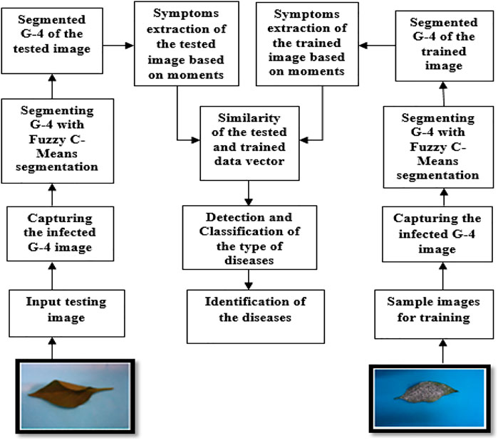
FIGURE 1. System flowchart to detect disease in chili plants.

Methodology

The methodology of the proposed system to detect different symptoms to check for plant infection is given below (Hemanth et al., 2019; Ramya et al., 2015).

Image Collection

Images were attained from the fields of G-4 (Guntur-4) variety chili plants, which in this case were from the I.C.A.R (Indian Council of Agricultural Research) (Hemanth et al., 2019). Scientists and associate researchers prepared the fields of the variety of plants that gets affected every year to find out the cause of the infection so that the farmers do not suffer a terrible produce. Chili leaf images were captured using a digital camera in a mini photo box of 30 cm * 45 cm * 35 cm. A total of 7,850 digital images of G-4 variety of chili leaves were captured, out of which 1,554 images were of bacterial leaf spot infection, 1,568 of powdery mildew (whitefly), 1,570 of chili leaf curl, 1,577 of Fusarium wilt (yellow), and 1,581 of healthy leaves.

The total data set of 7,850 images of chili leaves was divided into 5,000 images used as a training set and 2,850 images used for testing (Sufola et al., 2020). So the proposed method was tested on the data set to distinguish between these five different classes so as to identify the G-4 variety chili leaves to their respective class (Sufola et al., 2020).

Pre-Processing

The image was resized to 256 × 256 pixel (Dey et al., 2014). Upon resizing, the image was passed through a Gaussian filter to overcome any noise present (Pandian et al., 2019).

The RGB image was converted to HSV in order to make the disease identification easier (Pandian et al., 2019). Figure 2 shows the preprocessing cycle for the G-4 chili leaf input image, resized, filtered, and RGB to HSV converted.

FIGURE 2

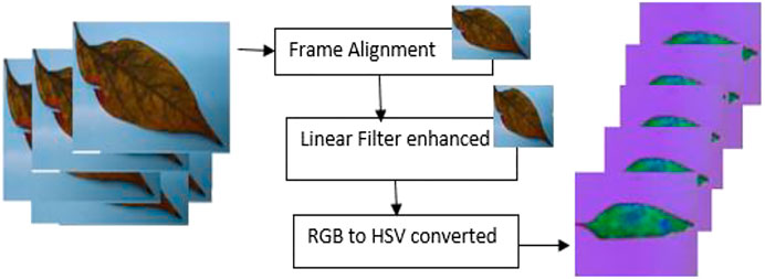
FIGURE 2. G-4 chili leaf input image, resized, filtered, and HSV.

Image Segmentation

The images which were obtained were given as input to a segmentation algorithm (Nandibewoor and Hegadi, 2019). Segmentation of an image is clustering similar property pixels into one cluster (Sufola et al., 2016a; Sufola et al., 2019; Ramya et al., 2015). The segmentation was done so that the image was represented in a more meaningful way so that it became easier to analyze (Sufola et al., 2018). Segmentation was done to separate the wanted part of the image from the background (Nandibewoor and Hegadi, 2019). Segmentation helps to distinguish the region of interest from the background of the image. The segmentation and clustering algorithm used was fuzzy c-means (FCM).

Fuzzy C-Means Segmentation Algorithm

Step 1: Number of clusters, the fuzzy parameter (a constant >1), and the stopping condition are set.

Step 2: Fuzzy partition matrix is initialized.

Step 3: Loop counter is set.

Step 4: Cluster centroids and the objective value J are computed.

Step 5: Membership values in the matrix are computed.

Step 6: When the value of J between iterations is less than the predefined stopping condition, stop, or else, increment k and go to step 4.

Step 7: De-fuzzification and segmentation.

The fuzzy c-means algorithm extracted the region of interest from the chili leaf image, where the object needed is a member of multiple clusters, with degrees of membership changing between 0 and 1 in FCM (Sufola et al., 2016b; Singh & Misra, 2017; Dey et al., 2014).

Trained Images

It is a data set of images which had different types of images of the infected and not infected leaves of the G-4 (Guntur-4) variety chilies. A total of 5,000 images out of 7,850 images were used as the training data set. These images were used to create the feature vector for training the proposed method.

Testing Data Images

The remaining 2,850 images from 7,850 were used as the testing data set. These images were from all five classes: bacterial leaf spot, powdery mildew (whitefly), chili leaf curl, Fusarium wilt (yellow), and healthy leaves.

Testing was done on the image to check if it was of any of the five types of chili leaves. The feature vector of these images was compared against the standard trained feature vector in the feature vector dataset.

Feature Extraction

This was a very important phase of this project. Feature extraction includes morphological operations (Pandit et al., 2015). The features are based on shape, color, and size (Sapna and Renuka, 2017). It extracts some important information of the object of interest (Titlee et al., 2017).

The feature vector of the trained image and the feature vector obtained from the test image were compared (Leeson, 2003; Ramya et al., 2015). The features were obtained by calculating the moments of each region. The following are the steps to calculate feature vector:

Dividing the Image Into Regions

Calculate area of each region.

Calculate the number of x-coordinate pixels and y-coordinate pixels of each region.

Calculate x- and y-centroids of each region.

Calculate x- and y-centroids of entire image.

Dividing the Image Into Regions

After segmenting the image, the image was divided into regions. This step is needed since it makes it easy to get the region of interest. It also becomes easier to get the area and centroid of the region of interest.

Calculating Area of Each Region

Here, we count the number of pixels which satisfies some condition.

The formula for it is as follows:

$area={\displaystyle \sum f}\left(x,y\right)\left\{\frac{+1 if(g<90\&\&r>5\&\&b>5)}{+0 if(g<90\&\&r>5\&\&b>5)}\right\},$

where f (x, y) is the measure of the pixel at coordinates x and y (Dhivyaprabha et al., 2018) and x is the height and y is the width of each block made of g (green), r (red), and b (blue) measures of pixels (Mothkur & Poornima, 2018; Persson & Åstrand, 2008).

1) Calculate the number of x-coordinate pixels and y-coordinate pixels

Here, we are summing up all the values of x-coordinate pixels and y-coordinate pixels, which satisfy the above condition.

2) Calculating x-centroid and y-centroid of each region

The center along the x and y axes of each region is calculated.

The following is the formula to calculate the x-centroid of each region:

$xcentroid=\left(\frac{sumx}{area}\right),$

where sumx is the number of pixels in the x-coordinate and area is the area of each region.

The following is the formula to calculate the y-centroid of each region:

$ycentroid=\left(\frac{sumy}{area}\right),$

where sumy is the number of pixels in the y-coordinate and area is the area of each region.

3) Calculating the x-centroid and y-centroid of the entire image

Here, it calculates the x-centroid and y-centroid of the entire image region.

4) Calculating the feature vector

Here, we are calculating the feature vector. Feature vector is the vector of moments.

Moments:

Image moment is the average or moment of an image pixel’s intensities or moment function, which usually has some properties related to the image. These properties can be area, centroid, and so on. Moments are suitable in shape learning. Zero to second order moments are applied for shape learning and orientation (Jacobs and Bean, 1963).

The formula to calculate moment is as follows:

$mpg={\displaystyle \sum }_x{\displaystyle \sum }_y{x}^p{y}^q.$

Here, p, q = 0,1,2. x = (number of x-coordinate pixel)–(xloc) (Gabriel, 2010). y = (number of y-coordinate pixel)–(yloc) (Gabriel, 2010).

The zeroth order moment gives the information of the area in the foreground, or it counts the total number of pixels in the region of interest.

M₁₀ is the measure of first order moment at x-axis (Pradhan and Deepak, 2016; Titlee et al., 2017; Schoeffmann et al., 2006; Adams et al., 2018).

M₀₁ is the measure of first order moment at y-axis (Pradhan and Deepak, 2016; Titlee et al., 2017; Schoeffmann et al., 2006; Adams et al., 2018).

M₂₀ is the measure of second order moment at x-axis (Adams et al., 2018; Schoeffmann et al., 2006).

M₀₂ is the measure of second order moment at y-axis (Adams et al., 2018; Schoeffmann et al., 2006).

Feature Vector Data Set

It is the data set which had the name of the infection, the file path, and the feature of that infected image.

Similarity of Regions

The symptoms of the images stored as feature vectors in the trained database were compared to the feature vector generated from the image under test to obtain a match. The feature vector of the test image was associated with the feature vector of the different infected images in the trained image feature data set. To relate the two feature vectors, the coefficient of correlation (CoC) of the two feature vectors was calculated.

Coefficient of correlation helps in judging resemblances between two measured vector quantities, while analyzing whether the two quantities are identical or completely different. Pearson’s correlation coefficient is denoted as r and is used in shape learning and computer image identification (Kaur et al., 2012; Anilkumar et al., 2020) (Anilkumar et al., 2020).

Steps to calculate the coefficient of correlation are as follows:

Considering two feature vectors u,v.

(1) Finding the average of the two feature vectors u,v.

(2) Calculating the difference vector of u,v.

(3) Calculating unit vector.

(4) Calculating correlation (similarity) of the two unit vectors.

(1) Finding the average of the two feature vectors u,v. We determine the average of the feature vectors by using

$\overline{u}=\left(\frac{{{\displaystyle \sum }}_1{u}_i}{n}\right).$

n = Quantity of values in vector u (Pandian et al., 2019); i = I, 2, 3 …n (Pandian et al., 2019).

$\overline{v}=\left(\frac{{{\displaystyle \sum }}_i{v}_i}{n}\right).$

n = quantity of values in vector v; i = 1, 2, 3 … n (Dhivyaprabha et al., 2018).

(2) Calculating the difference vector of u,v.

Here, we subtract each element of the feature vector from the average of the feature vector.

The formula to find the difference vector for feature vector u is as follows:

$\left\{u\right\}-\overline{u}.$

The formula to find the difference vector for feature vector v is as follows:

$\left\{v\right\}-\overline{v}.$

Here {u} is symptom vector (Zhou et al., 2015). {v} is symptom vector (Zhou et al., 2015). $\overline{u}$ is the average symptom vector u (Hsiao, 2007). $\overline{v}$ is the average symptom vector v (Hsiao, 2007).

(3) Calculating unit vector.

Here, we calculate the unit vector, which is the difference vector divided by the length.

The formula for calculating the length of the vector u is as follows:

$\left|u\right|=\sqrt{u_1^2+u_2^2+\dots +u_n^2}.$

Here, $\left|u\right|$ is the length of the u vector. $u_1^2+u_2^2+\dots +u_n^2$ is the element of the vector u.

The formula for computing the dimension of the vector v is as follows:

$\left|v\right|=\sqrt{v_1^2+v_2^2+\dots +v_n^2}.$

Here, $\left|v\right|$ is the length of the v vector. $v_1^2+v_2^2+\dots +v_n^2$ is the element of the vector v.

The formula to calculate the unit vector of the symptom vector u is as follows:

$\frac{\left\{\left\{\mathit{u}\right\}-\overline{\overline{\mathit{u}}}\right\}}{\left|\mathit{u}\right|}.$

Here, $\left\{\left\{u\right\}-\overline{\overline{u}}\right\}$ is the difference vector of symptom vector u. $\left|u\right|$ is the size of the symptom vector u (Zhou et al., 2015; Sapna and Renuka, 2017).

To evaluate the unit vector v, we use

$\left(\frac{\left\{\left\{v\right\}-\overline{\overline{v}}\right\}}{\left|v\right|}\right),$

$\left\{\left\{v\right\}-\overline{\overline{v}}\right\}$ is the difference vector of symptom vector v (Zhou et al., 2015; Sapna and Renuka, 2017). $\left|v\right|$ is the size of the symptom vector v (Zhou et al., 2015; Sapna and Renuka, 2017).

(4) Calculating correlation (similarity) of the two unit vectors.

The dot product of the unit vectors is calculated by using (Zhou et al., 2015; Sapna and Renuka, 2017)

$\left(\frac{\left\{\left\{u\right\}-\overline{\overline{u}}\right\}}{\left|u\right|}•\frac{\left\{\left\{v\right\}-\overline{\overline{v}}\right\}}{\left|v\right|}\right),$

$\left\{\left\{u\right\}-\overline{\overline{u}}\right\}$ is the difference vector of feature vector u. $\left|u\right|$ is the length of the feature vector u (Sapna and Renuka, 2017; Zhou et al., 2015). $\left\{\left\{v\right\}-\overline{\overline{v}}\right\}$ is the difference vector of feature vector v (Zhou et al., 2015). $\left|v\right|$ is the length of the feature vector v (Adams et al., 2018; Zhou et al., 2015). If the calculated coefficient of correlation is equal to 1, then the two images are absolutely identical (Kaur et al., 2012; Sapna and Renuka, 2017; Adams et al., 2018). If the calculated coefficient of correlation is equal to 0, then the two images are completely uncorrelated (Kaur et al., 2012). If the coefficient of correlation is calculated as value equal is –1, then the two images are completely anti-correlated (Kaur et al., 2012; Sapna and Renuka, 2017).

Experimental Results and Comparisons

The images of the different types of infected leaf images of the G-4 (Guntur-4) variety before and after segmentation of powdery mildew (whitefly) and Fusarium wilt (yellow) are displayed below (Wang & Chu, 2009; Jung et al., 2017).

Figures 3A,B are the images from before and after segmentation of powdery mildew (whitefly), and Figures 4A,B are the images from before and after segmentation of Fusarium wilt (yellow).

FIGURE 3

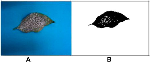
FIGURE 3. (A) Original G-4 chili powdery mildew (whitefly) leaf and (B) FCM-segmented chili powdery mildew (whitefly) leaf. Example images acquired after segmentation of (A,B).

FIGURE 4

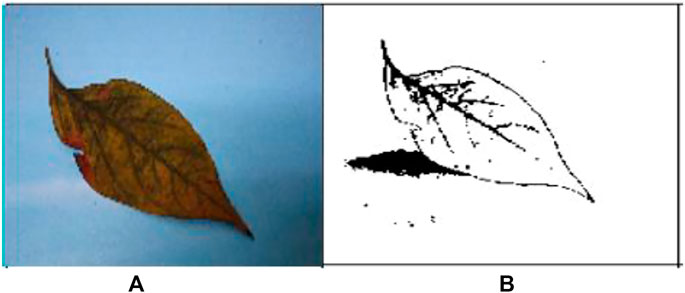
FIGURE 4. (A) Original G-4 chili Fusarium wilt (yellow) leaf and (B) FCM-segmented chili Fusarium wilt (yellow) leaf.

Table 1 shows the distribution of the total data set acquired, of the diseased G-4 chilli plant images.

TABLE 1

TABLE 1. Acquisition and distribution of the total dataset of disease in G-4 chili plants.

Table 2 shows the feature vector of each type of leaf image extracted based on moments.

TABLE 2

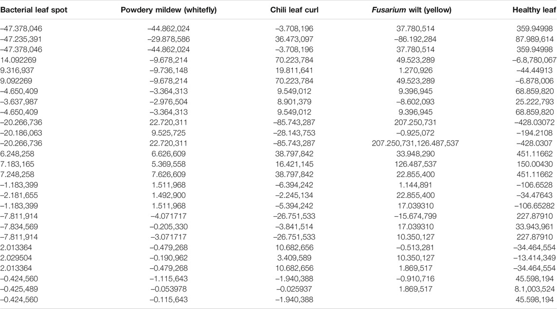
TABLE 2. Moment—symptoms/features extracted of G-4 leaf images.

Tables 3, 4 show the performance analysis using evaluation metrics (Sufola et al., 2016c). The result of testing shows that the proposed technique has an accuracy of 97.56%.

TABLE 3

TABLE 3. Performance analysis using evaluation metrics.

TABLE 4

TABLE 4. Performance analysis using evaluation metrics.

Figure 5 shows the evaluation matrices of the support vector machine technique and the moments technique used.

FIGURE 5

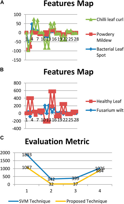
FIGURE 5. Evaluation metrics of the techniques. (A): Feature map of bacterial leaf spot, powdery mildew (whitefly), and chili leaf curl. (B): Feature map of Fusarium wilt (yellow) and healthy leaf.

Figure 6 the representation of the performance analysis of both the techniques used.

FIGURE 6

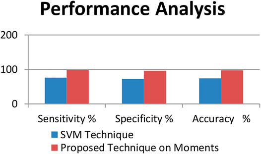
FIGURE 6. Performance analysis of the techniques.

Conclusion

Identification and detection of disease in G-4 (Guntur-4) variety chili leaves are useful for the farmers for detecting the diseases (Sufola et al., 2016d). The proposed system will reduce the errors which can occur during manual detection of diseases (Barolli et al., 2020).

This proposed system would be useful for farmers and scientists for fast detection of diseases. The above study shows that the proposed technique identifies the G-4 chili leaf diseases with an accuracy of 97.56%.

Data Availability Statement

The original contributions presented in the study are included in the article/Supplementary Material. Any further inquiries can be directed to the corresponding author.

Author Contributions

The authors are my guide and coguide, and they helped collect the samples from the Indian Council of Agricultural Research (ICAR) and carry out the research.

Conflict of Interest

The authors declare that the research was conducted in the absence of any commercial or financial relationships that could be construed as a potential conflict of interest.

References

Adams, S., Graham, C., Bolcavage, A., McIntyre, R., and Beling, P. A. (2018). “A Condition Monitoring System for Low Vacuum Plasma Spray Using Computer Vision”. in proceeding IEEE International Conference on Prognostics and Health Management (ICPHM). doi:10.1109/icphm.2018.8448464

CrossRef Full Text | Google Scholar

Anilkumar, K. K., Manoj, V. J., and Sagi, T. M. (2020). A Survey on Image Segmentation of Blood and Bone Marrow Smear Images with Emphasis to Automated Detection of Leukemia. Amsterdam, Netherlands: Elsevier B.V. Poland.

Barolli, L., Takizawa, M., Xhafa, F., and Enokido, T. (2020). Web, Artificial Intelligence and Network Applications. Springer Science and Business Media LLC.

Dey, N., Nandi, B., Bardhan Roy, A., Biswas, D., Das, A., and Chaudhuri, S. (2014). Chapter 17 Analysis of Blood Smear and Detection of White Blood Cell Types Using Harris Corner. Switzerland: Springer Nature.

Dhivyaprabha, T. T., Jayashree, G., and Subashini, P. (2018). “Medical Image Denoising Using Synergistic Fibroblast Optimization Based Weighted Median Filter,” in Second International Conference on Advances in Electronics, Computers and Communications (Bangalore, India: ICAECC). doi:10.1109/icaecc.2018.8479516

CrossRef Full Text | Google Scholar

Gabriel, S. (2010). Beginning Google Maps API 3. Springer Science and Business Media LLC.

Hemanth, D., Jude, B., and Valentina, E. (2019). Nature Inspired Optimization Techniques for Image Processing Applications. Springer Science and Business Media LLC.

Hsiao, M. H. (2007). Searching the Video: An Efficient Indexing Method for Video Retrieval in Peer to Peer Network. Hsinchu, Taiwan: Chiao Tung university.

Jacobs, I. S., and Bean, C. P. (1963). “Fine Particles, Thin Films and Exchange Anisotropy (Effects of Finite Dimensions and Interfaces on the Basic Properties of Ferromagnets),” in Magnetism. Editors G. T. Rado, and H. Suhl (New York: Academic), 3, 271–350. doi:10.1016/b978-0-12-575303-6.50013-0

CrossRef Full Text | Google Scholar

Jung, H. W., Lee, S. H., Martin, D., Parsons, D., and Lee, I. (2017). Automated Detection of Circular Marker Particles in Synchrotron Phase Contrast X-Ray Images of Live Mouse Nasal Airways for Mucociliary Transit Assessment. Adelaide, SA: Expert Systems with Applications, 25. doi:10.1016/j.eswa.2016.12.026

Kaur, A., Kaur, L., and Gupta, S. (2012). Image Recognition Using Coefficient of Correlation and Structural SIMilarity Index in Uncontrolled Environment”. Int. J. Comp. Appl. 59 (5). doi:10.5120/9546-3999

CrossRef Full Text | Google Scholar

Leeson, J. J. (2003). “Novel Feature Vector for Image Authentication”, in Proceeding of International Conference on Multimedia and Expo ICME 03 Proceedings (Cat No 03TH8698) ICME-03.

Google Scholar

Mothkur, R., and Poornima, K. (2018). “Machine Learning Will Transfigure Medical Sector”, A Survey, 2018 International Conference on Current Trends towards Converging Technologies. (Coimbatore, India: ICCTCT). doi:10.1109/icctct.2018.8551134

CrossRef Full Text | Google Scholar

Nandibewoor, A., and Hegadi, R. (2019). A Novel SMLR-PSO Model to Estimate the Chlorophyll Content in the Crops Using Hyperspectral Satellite Images. Cluster Comput. 22. 443–450. doi:10.1007/s10586-018-2243-7

CrossRef Full Text | Google Scholar

Pandian, D., Fernando, X., Baig, Z., and Shi, F. (2019). , in Proceeding of the International Conference on ISMAC in Computational Vision and BioEngineering 2018 (ISMAC-CVB). Springer Science and Business Media LLC.

Pandit, A., Kolhar, S., and Patil, P. (2015). Survey on Automatic RBC Detection and Counting. Int. J. Adv. Res. Electr. Elect. Instrumentation Eng. 4 (1), 1386–7857. doi:10.15662/ijareeie.2015.0401012

Google Scholar

Persson, M., and Åstrand, B. (2008). Classification of Crops and Weeds Extracted by Active Shap Models. Amsterdam, Netherlands: Elsevier Ltd.

Pradhan, A., and Deepak, B. B. V. L. (2016). Design of Intangible Interface for Mouseless Computer Handling Using Hand Gestures. Mumbai, India: Procedia Computer Science.

Ramya, M. C., Lokesh, V., Manjunath, T. N., and Hegadi, R. S. (2015). A Predictive Model Construction for Mulberry Crop Productivity. Proced. Comp. Sci. 45, 156–165. doi:10.1016/j.procs.2015.03.108

CrossRef Full Text | Google Scholar

Sapna, S., and Renuka, A. (2017). Techniques for Segmentation and Classification of Leukocytes in Blood Smear Images - A Review. IEEE International Conference on Computational Intelligence and Computing Research (ICCIC). doi:10.1109/iccic.2017.8524465

CrossRef Full Text

Schoeffmann, K., Merialdo, B., Hauptmann, A. G., Ngo, C. W., Andreopoulos, Y., and Breiteneder, C. (2006). Advances in Multimedia Modeling. Springer Science and Business Media LLC.

Singh, V., and Misra, A. K. (2017). Detection of Plant Leaf Diseases Using Image Segmentation and Soft Computing Techniques. China: Elsevier B.V.

Sufola, A., Meenakshi Sundaram, K., and Malemath, V. S. (2016d). “An Optimized Approach for Enhancement of Medical Images,” in Biomedical Research 7th September 2016, “An International Journal of Medical Sciences” (London, United Kingdom: Thompson Reuters Index Journal). 0970–938X. Special Issue: S283-S286.

Google Scholar

Sufola, A., Meenakshi Sundaram, K., and Malemath, V. S. (2020). “Automated Disease Identification in Chili Leaves Using FCM and PSO Techniques”. in RTIP2R 2020, “International Conference on Recent Trends in Image Processing and Pattern Recognition “in Communication in Computer and Information Science (CCIS) (Springer). SCOPUS INDEXED July 2020.

Google Scholar

Sufola, A., Meenakshi Sundaram, K., and Malemath, V. S. (2016c). “Chest CT Scans Screening of COPD Based Fuzzy Rule Classifier Approach”. in International Conference on “Advance in Signal Processing and Communication-SPC 2016” (Hyderabad, India: Proceedings published by WALTER De GRUYTER).

Google Scholar

Sufola, A., Meenakshi Sundaram, K., and Malemath, V. S. (2016a). Comparative Analysis of K-Means and K-Nearest Neighbor Image Segmentation Techniques. IEEE 6th International Conference on Advanced Computing(IACC). IEEE Conference Publications. doi:10.1109/IACC.2016.27

CrossRef Full Text | Google Scholar

Sufola, A., Meenakshi Sundaram, K., and Malemath, V. S. (2019). “Malemath “Detection and Segmentation of Blood Cells Based on Supervised Learning,” in International Journal of Engineering and Advanced Technology (IJEAT) (Madhya Pradesh, India: Journal Papers In Web Of Sci/Scopus). 9. 2249–8958.1S3

Google Scholar

Sufola, A., Meenakshi Sundaram, K., and Malemath, V. S. (2018). “Recognition and Detection of Object Using Graph-Cut Segmentation”. in “7th World Conference on Applied Sciences, Engineering & Management (WCSEM)” Organized by American Business School of Paris, France during 26-27 October 2018. Proceedings ISBN 13: 978-81-930222-3-8. Hyderabad, India: SCOPUS Indexed International Journal of Engineering and Technology, 2227–524X.

Google Scholar

Sufola, A., Meenakshi Sundaram, K., and Malemath, V. S. (2016b). Vegetable-Fruit Identification Based on Intensity and Texture Segmentation" in Special Issue of SCOPUS INDEX JOURNAL Titled. Int. J. Control. Theor. Appl. 0974–5572.

Google Scholar

Sulistyo, I. A., Isnanto, R. R., and Riyadi, M. A. (2020). “Size-based Feature Extraction on Blood Cells Calculation Process Using K-Means Clustering”. 7th International Conference on Information Technology, Computer, and Electrical Engineering (ICITACEE). doi:10.1109/icitacee50144.2020.9239248

CrossRef Full Text | Google Scholar

Titlee, R., Ur Rahman, A., Zaman, H. U., and Abdur Rahman, H. (2017). “A Novel Design of an Intangible Hand Gesture Controlled Computer Mouse Using Vision Based Image Processing”. 3rd International Conference on Electrical Information and Communication Technology (EICT). doi:10.1109/eict.2017.8275171

CrossRef Full Text | Google Scholar

Wang, M., and Chu, R. (2009). A Novel White Blood Cell Detection Method Based on Boundary Support Vectors. IEEE International Conference on Systems, Man and Cybernetics. doi:10.1109/icsmc.2009.5346736

CrossRef Full Text

Zhou, H., Huang, Y., Huang, S., Chen, K., Zhang, Y., and Feng, Z. (2015). Comprehensive Time-Frequency-Spatial Spectrum Measurement and Analysis of TV Band in Beijing. IEEE Wireless Communications and Networking Conference.