Three-dimensional catheter tip force sensing using multi-core fiber Bragg gratings

1 Introduction

1.1 Medical overview

Cardiovascular diseases (CVDs) are the leading cause of global mortality (Roth et al., 2020). Coronary artery diseases, heart attacks and arrhythmias are the most common CVDs. Atrial Fibrillation (AFib) is a type of CVD that affects around 59.7 million patients globally (Li et al., 2022). A common treatment of AFib is through ablation and scarring of cardiac tissue with the aim of impeding occurrences of irregular contraction waves (Calkins et al., 2009). Atrial ablation is usually performed by minimally invasive catheterization approaches (Lairikyengbam et al., 2003). In a consensus paper, Calkins et al. established the superior safety and efficacy of catheter-based approaches compared to open surgical approaches (Calkins et al., 2012). Although minimally invasive, catheter ablation is not free of risks. When too large forces are applied, complications such as cardiac perforation, cerebrovascular accidents and atrio-esophaegeal fistula may arise (Sra, 2008; Tang, 2017). On the other hand, applying too low forces during ablation may lead to unsuccessful scaring of the cardiac tissue, which in turn, may require for a repetition of the procedure. Zhou et al. recommends a contact force between 0.1–0.4 N for effective ablation (Zhou et al., 2017). However, given that the friction force between the catheter and the access port is an order of magnitude larger than the force between the ablation tip and the cardiac tissue, it is physically impossible for the electrophysiologist to perceive this latter contact force (Song et al., 2018). In this regard, the intricacy of catheter ablation procedures calls for high resolution and accurate contact force sensors.

1.2 Prior works

Several contact force sensors have been developed in the past for cardiac ablation catheters. Polygerinos et al. worked on different force sensor designs based on light intensity modulation (LIM). The sensors were primarily comprised of one or more optical fibers that were assembled in the direction of a reflector that is attached to a flexure. In their latest work (Polygerinos et al., 2013), Polygerinos et al. developed a 4 × 24.5 mm (outer diameter × length) force sensor with three separate fibers that was able to measure three-dimensional forces. The reported root mean square (RMS) force estimation error for the longitudinal and lateral cases was 30 mN and 21 mN, respectively. The force resolution was reported to be $lessbin10$ mN. Following a similar approach, Noh et al. designed a 3.5 × 13 mm three-dimensional force sensor based on LIM, three separate fibers, and a CCD camera (Noh et al., 2016). The reported maximum force estimation error for the longitudinal and lateral cases was 65 mN and 205 mN, respectively. The main limitations of approaches based on LIM is that they are prone to light intensity fluctuations and phase discontinuities (Abushagur et al., 2014; He et al., 2014). This may significantly affect the measurements and subsequently the force estimations. Furthermore, in the work of Noh et al., the force sensor was also observed to have notable longitudinal and lateral force coupling effects. The advantage of LIM based sensors, however, is that the light intensity is insensitive to the environmental temperature (Noh et al., 2016), meaning that temperature compensation is not necessary. An alternative approach to LIM relies on fiber Bragg grating (FBG) sensors inscribed within an optical fiber. Gao et al. developed a 2.6 × 11 mm three-dimensional force sensor based on four separate fibers with inscribed FBGs and parallel flexures (Gao et al., 2018). The sensor was reported to have RMS force estimation errors for the longitudinal and lateral cases of 7.94 mN and 13.6 mN, respectively. The sensor was also reported to have force resolutions for the longitudinal and lateral cases of 1.27 mN and 1.96 mN, respectively. The limitation of the sensor is that it involves a complex manufacturing and assembly procedure in addition to having potential FBG chirp failure which is caused by the non-uniform strain distribution on the adhesion zone (Li et al., 2020). Shi et al. developed a 4 × 18 mm two-dimensional force sensor based on four optical fibers with inscribed FBGs and a symmetric flexure, yielding a force resolution of 4.6 mN (Shi et al., 2018). The reported maximum force estimation errors, under constant temperature, was 250 mN. Besides being able to only measure lateral forces, another limitation of the force sensor was that it had bare fibers making it prone to breakage and unwanted interactions with the environment. Moreover, temperature compensation was inadequate yielding large force estimation errors with varying temperatures. Shin et al. designed a 2.3 mm outer diameter three-dimensional force sensor based on three separate FBG-inscribed fibers (Shin et al., 2018). The limitations of the force sensor are agian related to complex manufacturing and the potential for FBG chirping failure. Finally, Li et al. developed a 4 × 20 mm three-dimensional force sensor with five separate FBG-inscribed fibers and a miniature flexure (Li et al., 2020). The reported maximum force estimation error for the longitudinal and lateral cases was 24 mN and 15.6 mN, respectively. The reported force resolution for the longitudinal and lateral cases was 0.63 mN and 0.64 mN, respectively. Their force sensor displays a high performance and adequate temperature compensation. However, the limitations of the force sensor is that it uses too many optical fibers (i.e., five fibers), has a complex manufacturing and assembly process, and has relatively large dimensions. As can be seen, prior works utilize a combination of independent fibers in the design of the force sensor. This is usually done to decouple between lateral and longitudinal forces or to achieve temperature compensation. The reader is referred to (Polygerinos et al., 2010; Su et al., 2017) for an in-depth review on similar fiber optics based force sensors. Commercially, the most widely used catheters with tip contact force sensing are the Fabry-Perot interferometry-based TactiCath™ Quartz ablation catheter from Abbott (Chicago, IL, USA), and the magnetic transmitter/locator based Thermocool Smarttouch^® catheter from Biosense Webster (Irvine, CA, USA). Bourier et al. assessed the performance of both force sensors and found that they exhibit a mean force error of 11.8 mN and 58.8 mN, and a maximum force error of 49.0 mN and 294.2 mN, respectively (Bourier et al., 2016, 2017).

Note that the scope of force sensing, for medical applications, extends beyond catheter-based interventions. For example, various electrical-based sensors have been developed within minimally invasive surgery (MIS) to achieve tactile sensing of forceps and graspers (Bandari et al., 2020; Othman et al., 2022). Similarly, several force sensing concepts have been developed for needle tip force sensing (Liang et al., 2018). Note, however, that optical-based sensing techniques, and especially FBG-based techniques, are advantageous in comparison with other sensing methods as they comprise: 1) electromagnetic immunity, 2) miniature size, 3) high interrogation speed, 4) multiplexing capabilities, and 5) high mechanical strength (Taffoni et al., 2013; Shi et al., 2017).

1.3 Paper contributions and structure

In general, catheter tip force sensors may comprise functional or constructional limitations which include: non-linear measurement versus force output, force hysteresis, dimensional bulkiness, longitudinal and lateral force coupling effects, insufficient force estimation accuracy, and often complex designs or difficulty of assembly. In this paper, we propose the design of a novel catheter tip force sensor aiming to overcome all of the aforementioned limitations. The proposed sensor design is made to be simple, robust, and easily manufactured and assembled. The sensor design comprises a single multi-core fiber (MCF) with inscribed FBGs. This sensor embodiment avoids FBG chirping failure risks, fiber misalignments, and LIM-based limitations. The sensor embodiment also allows for redundant temperature compensation. To the best of the authors’ knowledge, this is the first implementation of a FBG-MCF for three dimensional force sensing. The developed force sensor is also integrated within an in-house built notched nitinol catheter that is actuatable through pneumatic artificial muscles (PAMs). This is done to prove the feasibility of integrating the force sensor within an actuatable catheter. It is important to note that the use of MCF technology not only allows for three-dimensional catheter tip force sensing, but also allows for a wide variety of other applications such as shape sensing (Moore and Rogge, 2012; Al-Ahmad et al., 2020), body force estimation (Aloi and Rucker, 2019; Al-Ahmad et al., 2021), and temperature monitoring. All of these capabilities can be integrated within a single catheter solution. This fits well with the targeted cardiac ablation application in this work (see Figure 1). The contributions of this paper are listed as follows.

• design and development of a novel catheter tip force sensor based on a multi-core fiber with inscribed FBGs,

• characterization and experimental validation of the force sensor using a dedicated experimental setup.

FIGURE 1

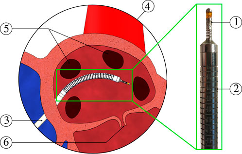
FIGURE 1. Catheter ablation scene: ① catheter tip force sensor, ② actuatable catheter, ③ medical delivery sheath, ④ zoomed-in view of the left atrium, ⑤ pulmonary veins, and ⑥ mitral valve.

The rest of this paper is organized as follows: Section 2 covers theoretical design aspects including helical spring theory, FBG strain sensing, and combined MCF and spring modelling. Section 3 focuses on the methodology for decoupling between longitudinal and lateral forces. Section 4 discusses different aspects related to the calibration of the force sensor. Section 5 presents the calibration results, sensor performance, and corresponding discussions. Finally, concluding remarks and future work aspects are provided in Section 6.

2 Force sensor design

The force sensor’s working principle is based on a single MCF inscribed with FBGs. A MCF differs from a single core fiber in that it contains a central core, but also circumferentially distributed outer cores at a given radial distance from the center (see Figure 4). All of the cores have FBGs inscribed into them meaning that strain can be sensed at different discrete locations along the MCF’s cross-section. The MCF is embedded within a helical compression spring which acts as the force-relaying flexure. The MCF is also rigidly attached to both ends of the spring to create a two-point fixation (see Figure 2). Temperature changes and external forces relayed to the MCF cause it to be strained internally. These internal strains are measured using the FBGs.

FIGURE 2

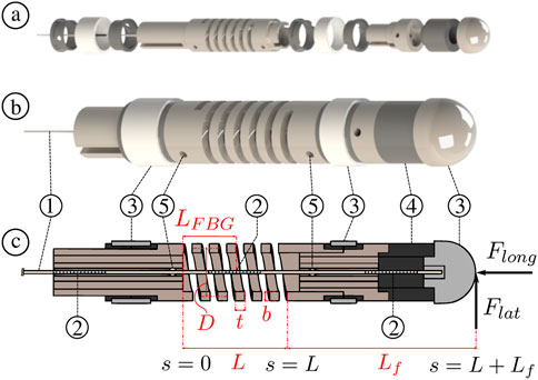
FIGURE 2. Force sensor overview ⓐ exploded view ⓑ assembled view ⓒ sectional view illustrating the relevant spring dimensions such as total length L, wire thickness t, wire breath b, and mean coil diameter D. The central FBG location along the spring’s length is given as L_FBG. The sensor’s components include: ① MCF, ② FBGs, ③ ablation electrodes, ④ insulation ring, and ⑤ side holes to inject adhesives for MCF fixation.

This section provides a theoretical approach towards the design and proper construction of the force sensor assembly. The theoretical approach provides the ability to customize and dimension the force sensor to achieve a user-defined performance. In this work, the force sensor is designed to achieve longitudinal and lateral force resolutions of $\le 1$ g (i.e., $\le 9.81\times 10^{-3}$ N), which is the targeted performance metric.

2.1 Helical spring theory

2.1.1 Longitudinal deflection

Figure 2C illustrates a sectional view of the force sensor with a helical compression spring having a total length L, wire thickness t, wire breath b, and mean coil diameter D. If an external longitudinal force F_long is applied onto the end of the spring, then the corresponding longitudinal deflection δ_long can be described as (Wahl, 1944):

${\delta }_{\mathit{long}}=\frac{D^3{N}_a}{K_{2}b{t}^{3}G}{F}_{\mathit{long}},(1)$

where N_a is the number of active coils, K₂ is a factor depending on the ratio b/t, and G is the spring material’s shearing modulus of rigidity. The expression in Eq. 1 can be rewritten into the common expression for a linear compression spring:

${\delta }_{\mathit{long}}=\frac{1}{K_{\mathit{long}}}{F}_{\mathit{long}},(2)$

where K_long is commonly known as the spring’s longitudinal stiffness. It can be seen that the free parameters b, t, D, N_a, and G dictate the spring’s longitudinal stiffness K_long, and thus the amount of force to be transmitted to the MCF.

2.1.2 Buckling

If a relatively large longitudinal force is exerted upon the spring, one that exceeds the spring’s critical buckling load F_cr, then the spring would buckle and be damaged permanently. Hence it is crucial to take the buckling load into account during the design phase. The compressive α, flexural β, and shearing γ rigidities of a helical compression spring are needed for its computation and are given as (Wahl, 1944):

$\alpha =\frac{K_{2}b{t}^{3}GL}{D^3{N}_a},(\mathrm{3a})$

$\beta =\frac{2EIG{I}_{p}L}{N_a\pi D\left(G{I}_p+EI\right)},(\mathrm{3b})$

$\gamma =\frac{8EIL}{N_a\pi D^3},(\mathrm{3c})$

Where E is the spring material’s modulus of elasticity, and I and I_p are the area and polar moments of inertia of the spring’s wire cross-section respectively. The spring’s critical buckling load F_cr is computed as (Wahl, 1944):

$F_{cr}=\frac{{\pi }^2\beta }{L{L}_1\left(1+\frac{{\pi }^2\beta }{{L_1}^2\gamma }\right)},(4)$

where L₁ is the critical length of the spring when F_cr is applied. Expression 4) can also be written in the form (Wahl, 1944):

$F_{cr}=\frac{L-L_1}{L}\alpha .(5)$

However, at this point L₁ is yet unknown. If μ is taken to be the ratio $\frac{L_1}{L}$, then substituting μ into 5) and subsequently into 4) gives the following expression:

${\mu }^3-{\mu }^2+\frac{\mu {\pi }^2\beta }{L^2}\left(\frac{1}{\gamma }+\frac{1}{\alpha }\right)-\frac{{\pi }^2\beta }{L^2\gamma }=0,(6)$

which is a cubic equation that can be solved for μ; note that 0 < μ < 1. The critical buckling load F_cr is found by computing L₁ through μ and substituting its value into 5).

2.1.3 Lateral bending

Consider the case where the force sensor is subjected to a lateral force F_lat at the tip which is at a distance L_f from the spring’s end, as depicted in Figure 2C. The part of the force sensor along L_f is rigid. Hence the lateral force F_lat at the tip leads to a combination of a lateral force F_lat,1 = F_lat and a bending moment M_lat,1 = F_latL_f at the spring’s end. If s is the arc length parameter from the spring’s base s = 0 to its end s = L, then the moment M(s) as a function of this arc length s can be given as:

$M\left(s\right)=F_{\mathit{lat}}\left(L+L_f-s\right).(7)$

Consequently, the parametrized curvature κ_s(s) as a function of s going from 0 to L is given in the following form:

${\kappa }_s\left(s\right)=\frac{M\left(s\right)}{\beta }=\frac{\left(L+L_f-s\right)}{\beta }{F}_{\mathit{lat}}.(8)$

The spring’s curvature κ_s is thus maximum at the base s = 0 and decreases linearly towards its end.

2.2 Strain sensing using FBGs

2.2.1 Overall strain sensing

FBGs detect variation of strain based on the change of periodicity and refractive index of the grating. The Bragg wavelength λ_B is the wavelength of the light that is reflected back from the grating. The change in strain can be a result of mechanical strain ϵ or thermal expansion due to temperature change ΔT. The change in Bragg wavelength Δλ_B depends on both effects and can thus be expressed as:

$\frac{{\lambda }_B-{\lambda }_{B_0}}{{\lambda }_{B_0}}=\frac{\mathrm{\Delta }{\lambda }_B}{{\lambda }_{B_0}}=S_{ϵ}\mathrm{\Delta }ϵ+S_T\mathrm{\Delta }T(9)$

where ${\lambda }_{B_0}$ is the grating’s unstrained Bragg wavelength, Δϵ is the change in mechanical strain with respect to the unstrained state, and S_ϵ and S_T are the strain and temperature sensitivity coefficients respectively.

2.2.2 Decoupling mechanical and thermal strains

The force sensor embodiment comprises three FBG sets as shown in Figure 2C. As will be elaborated in Section 2.3, the central FBG is mechanically constrained between the two ends of the spring. On the other hand, the leading and trailing FBGs are free and unconstrained. This means that the middle FBG is subjected to both mechanical strain Δϵ and temperature change ΔT, while the leading and trailing FBGs are only subjected to temperature change ΔT. Hence, measuring the wavelength shifts Δλ_B in the leading and trailing FBG sets allows computing ΔT (since Δϵ = 0) from Eq. 9, and consequently compensating for its effect in the middle FBG. This is done to isolate the mechanical strain Δϵ.

2.3 MCF and spring combination − longitudinal loading

2.3.1 Longitudinal deflection and stiffness

The MCF is rigidly fixed to both ends of the spring. In order to prevent the MCF from buckling during operation, pre-straining is applied a priori. The steps that are followed to apply a pre-strain on the MCF are illustrated in Figure 3 and described in the following.

① the spring is initially unloaded with its length equal to the free length L;

② a known longitudinal calibration force F_c is applied onto the spring, resulting in a deflection ${\delta }_c=\frac{F_c}{K_{\mathit{long}}}$;

③ the MCF is introduced and rigidly fixed to the ends of the spring using adhesives (see also Figure 2C); the calibration force F_c is still being applied and the deflection remains δ_c at this point;

④ after the adhesive cures, the calibration force F_c is removed and the spring/fiber combination reaches a new equilibrium with the deflection of the spring being δ_e.

At equilibrium, the internal force acting on the spring F_s is equal and opposite in direction to the internal force acting on the fiber F_f. Here, the total deflection of the spring is δ_e, while the total deflection of the fiber is δ_c − δ_e. Hence, the force balance at equilibrium is:

$K_{\mathit{long}}{\delta }_e=K_{\mathit{fib}}\left({\delta }_c-{\delta }_e\right),(10)$

where K_fib is the fiber’s longitudinal stiffness. This equilibrium state is considered as the unstrained reference state of the fiber, i.e., where λ_B,0 is defined and all future strain or wavelength changes are based upon. When an external longitudinal force F_long is applied and a new static equilibrium is reached, the following expression is obtained:

$F_{\mathit{long}}=K_{\mathit{long}}{\delta }_{\mathit{long}}-K_{\mathit{fib}}\left({\delta }_c-{\delta }_{\mathit{long}}\right),(11)$

where δ_long is the spring’s longitudinal deflection due to the longitudinal force F_long.

FIGURE 3

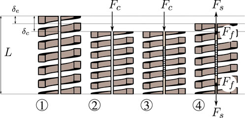
FIGURE 3. Illustration of the MCF pre-straining steps: ① the spring is fixed at the base and is initially free and unloaded, ② a longitudinal calibration force F_c is applied at the spring’s end, ③ the MCF is inserted into the spring and fixed at both ends with appropriate adhesives (the longitudinal calibration force F_c is still being applied at the spring’s end), ④ once the adhesive is fully cured, i.e., the end-points fixations are rigid, the longitudinal calibration force F_c is removed and the spring extends to an equilibrium position.

2.3.2 Working force range

Based on the nature of the targeted application, external forces are predominantly compressive. Proper functioning of the force sensor is thus primarily related to the buckling of either the helical spring or the MCF. Buckling of the helical spring is prevented by ensuring that the magnitude of the applied external forces are $<F_{cr}$. Similarly, buckling of the MCF is prevented by ensuring that the magnitude of the applied external forces are $<F_c$. As such, both F_cr and F_c determine the force sensor’s working range. In principle, F_c can be as large as F_cr. In practice, however, F_c is usually smaller than F_cr. The force sensor’s working range is thus determined by F_c and can be customized based on application and user requirements.

2.3.3 Longitudinal strain

The external longitudinal force F_long causing a spring deflection δ_long consequently corresponds to a fiber strain Δϵ_long. Given that the fiber’s initial length is L − δ_e, and its length after the application of the longitudinal force F_long is L − δ_long, the fiber’s longitudinal strain Δϵ_long is thus given as:

$\begin{array}{ll}\hfill & \mathrm{\Delta }{ϵ}_{\mathit{long}}=\frac{\left(L-{\delta }_{\mathit{long}}\right)-\left(L-{\delta }_e\right)}{L-{\delta }_e},\hfill \\ \hfill & =\frac{{\delta }_e-{\delta }_{\mathit{long}}}{L-{\delta }_e}.\hfill \end{array}(12)$

Considering that L ≫ δ_e, hence L ≈ L − δ_e, expression (12) can be simplified to:

$\mathrm{\Delta }{ϵ}_{\mathit{long}}=\frac{{\delta }_e-{\delta }_{\mathit{long}}}{L}.(13)$

Substituting (13) into 9) gives the longitudinal deflection δ_long due to the applied longitudinal force F_long from a measured wavelength shift Δλ_B:

${\delta }_{\mathit{long}}={\delta }_e-\frac{L}{S_{ϵ}}\left(\frac{\mathrm{\Delta }{\lambda }_B}{{\lambda }_{B_0}}-S_T\mathrm{\Delta }T\right).(14)$

By combining expressions (10), (11) and (14), and solving for F_long, the following expression is obtained:

$F_{\mathit{long}}=\left(K_{\mathit{long}}+K_{\mathit{fib}}\right)\frac{L}{S_{ϵ}}\left(S_T\mathrm{\Delta }T-\frac{\mathrm{\Delta }{\lambda }_B}{{\lambda }_{B_0}}\right).(15)$

If we consider that the temperature is constant or compensated, then expression (15) can be simplified to obtain the following longitudinal force F_long magnitude:

$F_{\mathit{long}}=\frac{\left(K_{\mathit{long}}+K_{\mathit{fib}}\right)L}{S_{ϵ}{\lambda }_{B_0}}\mathrm{\Delta }{\lambda }_B.(16)$

The magnitude of the externally applied longitudinal force F_long could thus be obtained via the linear relationship in Eq. 16 by measuring the wavelength shift Δλ_B.

2.3.4 Longitudinal force resolution

The wavelength shift Δλ_B within the MCF is usually measured using an optical interrogator. The interrogator, such as one based on wavelength division multiplexing (WDM), can measure wavelength shifts to a given resolution. The resolution is usually related to the interrogator’s hardware and the accuracy of the subsequent wavelengths peak detection algorithm. Accordingly, Λ_min is defined as the minimum detectable wavelength shift. The longitudinal force resolution Ω_long can thus be obtained by solving (16) and substituting Δλ_B with Λ_min such that:

${\mathrm{\Omega }}_{\mathit{long}}=\frac{\left(K_{\mathit{long}}+K_{\mathit{fib}}\right)L}{S_{ϵ}{\lambda }_{B_0}}{\mathrm{\Lambda }}_{\min }.(17)$

2.4 MCF and spring combination − lateral loading

2.4.1 Effective rigidity and curvature

Figure 2C illustrates how the fiber is fixed with respect to the helical spring. Ideally, the fiber is concentric and collinear with respect to the spring’s central longitudinal axis. The fiber is rigidly fixed to the ends of the spring using adhesives. Assuming equal curvature and relatively small deflections, the fiber and spring combination can be treated as a composite material having an effective flexural rigidity β_eff as (Denavit et al., 2018):

${\beta }_{\mathit{eff}}=E_{\mathit{fib}}{I}_{\mathit{fib}}+\beta ,(18)$

where E_fib and I_fib are the fiber’s modulus of elasticity and cross-sectional area moment of inertia respectively. Expression 8) can then be updated to include this composition for the effective curvature κ_eff:

${\kappa }_{\mathit{eff}}\left(s\right)=\frac{\left(L+L_f-s\right)}{{\beta }_{\mathit{eff}}}{F}_{\mathit{lat}}.(19)$

The position of the middle FBG, i.e., the FBG constrained between both ends of the spring, can be adjusted along the longitudinal axis of the spring before rigidly fixing it. This will define the arc length s at which wavelength and strain measurements are evaluated. If we consider the location of the FBG to be at s = L_FBG, i.e., the distance to the FBG’s center along its length, and take L_eff = L + L_f − L_FBG and κ_eff ≡ κ_eff (L_FBG), then the magnitude of the applied lateral force F_lat can be given as:

$F_{\mathit{lat}}=\frac{{\beta }_{\mathit{eff}}}{L_{\mathit{eff}}}{\kappa }_{\mathit{eff}}.(20)$

Expression (20) illustrates the linear relationship between the lateral force magnitude F_lat and effective curvature κ_eff.

2.4.2 Lateral force resolution

With reference to Figure 4, considering a MCF configuration with one central core and three equally distributed outer cores along a circumference with a radial distance r from the center, the relationship between measured strain ϵ and effective curvature κ_eff is (Moore and Rogge, 2012):

${\kappa }_{\mathit{eff}}=\frac{-{ϵ}_i}{r\text{cos}\left({\theta }_b-\frac{3\pi }{2}-{\theta }_i\right)},(21)$

where $i\in \left[\mathrm{1,2,3}\right]$ represents the ith outer core, θ_b is the angle of the bending plane normal vector, ${\theta }_i={\theta }_1+\frac{2\pi \left(i-1\right)}{3}$, and θ₁ is the angle between the center of the first outer core and a reference axis. The reference axis can be arbitrarily chosen but usually coincides with an externally identifiable geometric landmark. The magnitude of the measured effective curvature κ_eff can be found as follows (Moore and Rogge, 2012):

${\kappa }_{\mathit{eff}}=\frac{2}{3r}\sqrt{{\left({\sum }_{i=1}^3{ϵ}_i\text{cos}{\theta }_i\right)}^2+{\left({\sum }_{i=1}^3{ϵ}_i\text{sin}{\theta }_i\right)}^2}.(22)$

The angle of the bending plane normal vector θ_b can be obtained from the apparent curvature vector κ_app as given in (Moore and Rogge, 2012), and is used to divide the total curvature κ_eff into its orthogonal principal components. By replacing the expression for κ_eff from Eq. 22 into Eq. 20, the following is obtained:

$F_{\mathit{lat}}=\frac{2{\beta }_{\mathit{eff}}}{3r{L}_{\mathit{eff}}}\sqrt{{\left({\sum }_{i=1}^3{ϵ}_i\text{cos}{\theta }_i\right)}^2+{\left({\sum }_{i=1}^3{ϵ}_i\text{sin}{\theta }_i\right)}^2}.(23)$

Without loss of generality, a simplified geometrical case can be analysed to derive an overall estimate of the lateral force resolution Ω_lat. Here, the reference axis is considered to coincide with the first outer core, i.e., θ₁ = 0, and the bending plane coincides with the reference axis, i.e., ${\theta }_b=\frac{3\pi }{2}$. Due to symmetry, the sum of the outer core strains must be equal to zero, ${\sum }_{i=1}^3{ϵ}_i=0$. Given that the measured strain in the first outer core will be zero (since it falls along the neutral axis), the strains in the second and third outer cores will be equal in magnitude but opposite in direction such that ϵ₂ = −ϵ₃. The resulting relationship between the lateral force F_lat and measured strain ϵ₂ based on Eq. 23 is found to be:

$F_{\mathit{lat}}=\frac{2{\beta }_{\mathit{eff}}}{\sqrt{3}r{L}_{\mathit{eff}}}{ϵ}_2.(24)$

Similar to the longitudinal case, by substituting Δλ_B with Λ_min into 9), considering that the temperature is constant or compensated, and taking ϵ₂ = Δϵ, the following expression is found from Eq. 24 for the lateral force resolution Ω_lat:

${\mathrm{\Omega }}_{\mathit{lat}}=\frac{2{\beta }_{\mathit{eff}}}{\sqrt{3}r{L}_{\mathit{eff}}{S}_{ϵ}{\lambda }_{B,0}}{\mathrm{\Lambda }}_{\min }.(25)$

The longitudinal and lateral force resolutions, Ω_long and Ω_lat, could thus be customized by dimensioning the various sensor’s properties and geometry. Note that the force resolutions are not strictly decoupled and thus modification of one may have an effect on the other.

FIGURE 4

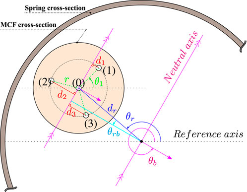
FIGURE 4. Cross-sectional view of the MCF and spring combination. The MCF’s center is at a radial offset d_r from the spring’s center and at an angular offset θ_r with respect to a reference axis. θ_b is the angle of the bending plane vector with respect to the reference axis and θ₁ is the angle between the center of the first outer core and the reference axis. r is the radial distance from an outer core to the central core, and d_i for $i\in \left[\mathrm{1,2,3}\right]$ is the perpendicular distance between the outer cores and the neutral axis crossing the central core. θ_rb is the angle between the bending plane vector θ_b − π and θ_r.

3 Decoupling longitudinal and lateral forces

3.1 Total strain

The MCF is ideally embedded coaxially with the spring’s longitudinal axis. However, it is a challenge to practically guarantee this. It therefore becomes necessary to compensate for any of the adverse effects that result from MCF and spring non-coaxiality. Figure 4 provides an illustrative schematic of the cross-sectional view of a general MCF and spring combination. The MCF’s center is at a certain radial offset d_r from the spring’s longitudinal axis and at an angular offset θ_r from the reference axis. The perpendicular distance between the line parallel to the neutral axis crossing the MCF’s central core and the spring’s longitudinal axis is given by d_r cos θ_rb, where θ_rb = θ_b − π − θ_r. The total measured strain in each of the MCF’s cores when both a longitudinal force F_long and a lateral force F_lat are applied can thus be given as follows:

${ϵ}_0={ϵ}_{\mathit{long}}+{ϵ}_{\mathrm{\Delta }T}+d_r\text{cos}{\theta }_{rb}{\kappa }_{\mathit{eff}},(\mathrm{26a})$

${ϵ}_i={ϵ}_{\mathit{long}}+{ϵ}_{\mathrm{\Delta }T}+d_r\text{cos}{\theta }_{rb}{\kappa }_{\mathit{eff}}-r\text{cos}\left({\theta }_b-\frac{3\pi }{2}-{\theta }_i\right){\kappa }_{\mathit{eff}},(\mathrm{26b})$

Where ϵ₀ is the strain in the central core, ϵ_i is the strain in the ith outer core for $i\in \left[\mathrm{1,2,3}\right]$, and ϵ_ΔT is the strain due to temperature change. As can be seen from (26), the common mode amongst all cores is measured with the central core and contains the effects from longitudinal strain ϵ_long, temperature change ϵ_ΔT, and offset from the neutral axis d_r cos θ_rbκ_eff.

3.2 Decoupling of strains

Without loss of generality, the reference axis will be chosen to be parallel with the line intersecting the MCF’s central and first outer cores such that θ₁ = 0. This is done to obtain a straightforward solution and avoid extra calibration to find θ₁. The assignment is possible since the choice of the direction of the reference axis can be arbitrarily defined. Accordingly, the remaining unknowns in (26) are the geometrical offsets d_r and θ_r. These parameters are found through calibration and least-squares fitting (as will be seen later in Section 4). Note that the curvature magnitude κ_eff, as defined in Eq. 22, and the direction of the bending plane normal vector θ_b are independent from the common mode. This is because their computation relies on the differences in strain between the outer cores and not on their absolute magnitude. Hence both κ_eff and θ_b can be independently computed from the outer core strains ϵ_i. This can then be used to compute the lateral force F_lat via Eq. 20. Note that the lateral force can be decomposed into its orthogonal principal components using the bend angle θ_b. As previously elaborated, the force sensor embodiment allows for the compensation of temperature changes by employing two extra unstrained FBGs. Since the FBGs are unstrained, i.e., Δϵ = 0, their measured wavelength shifts Δλ_B are used to compute temperature changes ΔT. The longitudinal strain ϵ_long could thus be computed from Eq. 26a, converted to a longitudinal wavelength shift Δλ_B,long using (9), and consequently used to compute the longitudinal force F_long from Eq. 16. In this manner, both F_long and F_lat can be computed separately and independently.

4 Sensor development and calibration

4.1 MCF pre-straining

Figure 5A illustrates the experimental setup used for MCF pre-straining. The force sensor body comprising the flexural spring is held firmly using a mechanical vice. A commercial six DoF Nano17 force/torque sensor (ATI Industrial Automation, Apex, NC, United States) is used to measure and apply the compressive calibration force F_c. The ATI force sensor is mounted onto a sliding block and a linear guide. A screw at the backside of the ATI force sensor is used for incremental displacement and control of the contact force. Once the desired calibration force F_c is applied, the screw is fixed in place and adhesives are applied onto the MCF and spring combination. The ATI force sensor is moved back and released once the two-point adhesive curing is complete.

FIGURE 5

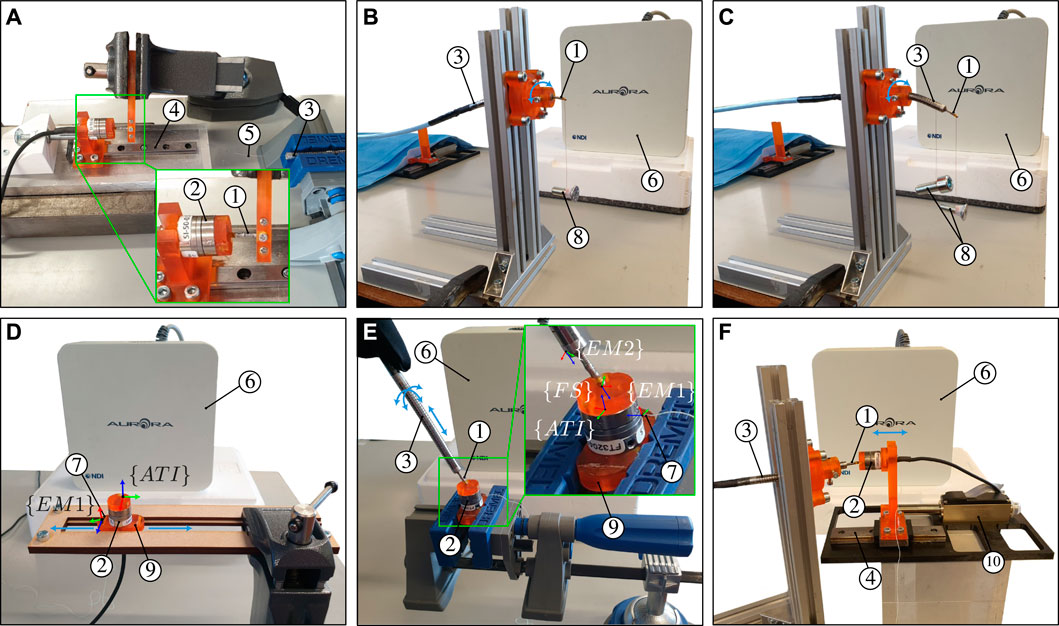
FIGURE 5. Illustration of the calibration and experimental setups for (A) MCF pre-straining through spring initial compression (B) identification of d_r and θ_r (C) identification of the angle between the x − axis of EM two and the first outer core of the MCF (D) identification of the angle between the x −axis of EM one and the y −axis of the ATI force sensor (E) three-dimensional catheter tip force sensor calibration, and (F) dynamic force characterization. The calibration and experimental setups contain the following elements: ① catheter tip force sensor, ② ATI Nano17 force sensor, ③ bendable and actuatable catheter, ④ linear guide, ⑤ MCF, ⑥ EM field generator, ⑦ EM two sensor, ⑧ hanging weights, ⑨ 3D printed rigid base, and ⑩ linear servomotor.

4.2 Computing offsets d_r and θ_r

Consider a configuration j, where the force sensor is clamped horizontally with a predominantly lateral force being applied at the tip in the direction of gravity, as shown in Figure 5B. Consider the exact same configuration j + 1 where the force sensor is rotated by an incremental amount about its longitudinal axis. From Eq. 26a, the strain relationship in the central core for those two configurations would be as follows:

${ϵ}_{0,j}={ϵ}_{\mathit{long,j}}+{ϵ}_{\mathrm{\Delta }T,j}+d_r\text{cos}{\theta }_{rb,j}{\kappa }_{\mathit{eff,j}},(\mathrm{27a})$

${ϵ}_{0,j+1}={ϵ}_{\mathit{long,j+1}}+{ϵ}_{\mathrm{\Delta }T,j+1}+d_r\text{cos}{\theta }_{rb,j+1}{\kappa }_{\mathit{eff,j+1}}.(\mathrm{27b})$

Given the axisymmetry of the spring and force sensor body, the curvature κ_eff should remain approximately constant between the two configurations such that κ_eff = κ_eff,j = κ_eff,j+1. Furthermore, the corresponding longitudinal strain in both configurations should also remain approximately the same, ϵ_long,j = ϵ_long,j+1. Finally, if the two configurations are achieved within a short period of time, or the environmental temperature is kept constant, then ϵ_ΔT,j = ϵ_ΔT,j+1. Comparing both configurations would thus yield:

${ϵ}_{0,j+1}-{ϵ}_{0,j}=d_r{\kappa }_{\mathit{eff}}\left(\text{cos}{\theta }_{rb,j+1}-\text{cos}{\theta }_{rb,j}\right).(28)$

Considering that there are N consecutive configurations differing by an incremental rotation about the force sensor’s longitudinal axis, then a vector Ψ with N − 1 elements can be constructed such that:

$\mathbf{\Psi }\left(j\right)={ϵ}_{0,j+1}-{ϵ}_{0,j}-d_r{\kappa }_{\mathit{eff}}\left(\text{cos}{\theta }_{rb,j+1}-\text{cos}{\theta }_{rb,j}\right),(29)$

where Ψ(j) is the jth element of Ψ. The geometrical offsets d_r and θ_r can be obtained through least-squares minimization of Ψ, i.e., $\min \left({\sum }_{j=1}^{N-1}{\mathbf{\Psi }(j)}^2\right)$. Note that d_r is constrained between $\left[0,d_{r,\max }\right]$, where d_r, max is the maximum possible central offset of the MCF within the spring, and θ_r is constrained between $\left[\mathrm{0,2}\pi \right]$.

4.3 Calibration matrix

Following from the relationships given in Eq. 16 and Eq. 20, it is clear that the longitudinal F_long and lateral F_lat forces vary linearly with the measurements Δλ_B,long and κ_eff, respectively. A coordinate frame is assigned to the force sensor such that the xy − axes fall on a plane with a normal in the direction of the spring’s longitudinal axis, and the z − axis points in the direction of that normal, from the base to the tip (see Figure 5E). Considering that F_x = F_lat,x, F_y = F_lat,y, and F_z = F_long, then the overall relationship between the output force and the input measurements is given as:

$\mathit{F}=\mathit{C}\mathbf{\Theta },(\mathrm{30a})$

$\left[\begin{array}{c}\hfill F_x\hfill \\ \hfill F_y\hfill \\ \hfill F_z\hfill \end{array}\right]=\left[\begin{array}{ccc}\hfill c_{11}\hfill & \hfill c_{12}\hfill & \hfill c_{13}\hfill \\ \hfill c_{21}\hfill & \hfill c_{22}\hfill & \hfill c_{23}\hfill \\ \hfill c_{31}\hfill & \hfill c_{32}\hfill & \hfill c_{33}\hfill \end{array}\right]\times \left[\begin{array}{c}\hfill {\kappa }_{\mathit{eff}}\text{cos}\left({\theta }_b\right)\hfill \\ \hfill {\kappa }_{\mathit{eff}}\text{sin}\left({\theta }_b\right)\hfill \\ \hfill \mathrm{\Delta }{\lambda }_{B,long}\hfill \end{array}\right],(\mathrm{30b})$

Where $\mathit{F}=\left[F_x\right.$, F_y, ${\left.F_z\right]}^T$, $\mathbf{\Theta }=\left[{\kappa }_{\mathit{eff}}\right.\text{cos}\left({\theta }_b\right)$, ${\kappa }_{\mathit{eff}}\text{sin}\left({\theta }_b\right)$, ${\left.\mathrm{\Delta }{\lambda }_{B,long}\right]}^T$, and C is the calibration matrix. The calibration matrix C is found from experimental calibration data for F and Θ and computed as C = FΘ⁺, where ⁺ represents the matrix pseudo-inverse.

4.4 Force calibration setup

Calibration of the force sensor requires 3D ground truth force data, obtained here by utilizing the commercial Nano17 force/torque sensor. A transformation of the measured 3D force from the Nano17 force sensor’s coordinate frame to the local frame of the developed force sensor is required however. This is achieved by using the setup shown in Figure 5E. Two EM sensors are employed here to establish the coordinate frame transformation between the Nano17 ground truth and catheter tip force sensors. The first EM is attached to a rigid base which in turn is attached to the Nano17 force sensor. The second EM is embedded within the notched tube catheter which in turn houses the developed force sensor. The transformations between the Nano17 force sensor and EM 1, and the developed force sensor and EM 2, are thus known and constant. The method to obtain these transformations is elaborated next.

4.4.1 Transformation from Nano17 to EM 1

The rigid base shown in Figure 5E is constructed such that the z − axis of the EM sensor is parallel with the x − axis of the Nano17 force sensor. This means that the xy plane of the EM sensor is parallel to the yz plane of the Nano17 force sensor. The angle between the x − axis of the EM sensor with respect to the xy plane of the Nano17 force sensor θ_x1, is required to fully define the rotational transformation from the Nano17 force sensor frame {ATI} to the EM sensor frame {EM1}. The rigid base has flat surfaces at opposite sides parallel to the xy plane of EM 1. Accordingly, the rigid base is placed in a slot constraining its movement exclusively along the y − axis of the Nano17 force sensor (see Figure 5D). The rigid base is moved back and forth within this slot while simultaneously measuring EM one position data. This generates a series of three-dimensional points through which a straight line can be fitted. Angle θ_x1 is then found by computing the angle between the x − axis of EM one and the fitted line.

4.4.2 Transformation from EM two to force sensor

The notched tube catheter shown in Figure 5E is constructed such that the z − axis of the EM sensor is parallel with the local z − axis of the developed force sensor. Accordingly, the notched tube catheter and force sensor assembly are clamped horizontally. A weight is attached to the notched tube catheter and a lighter weight is attached to the force sensor (see Figure 5C). Both the notched tube catheter and the force sensor would bend in the same direction due to gravity. A vector can then be constructed from the position of the EM when no weight is applied to the position of the EM when the weights are applied. This vector is projected onto the xy plane of the EM sensor and used to compute the angle between this vector and the x − axis of the EM sensor θ_x2. The process is repeated for different orientations, i.e., rotation about the longitudinal axis, to obtain better approximation of θ_x2. The x − axis of EM two and the line between the central and first outer core are aligned by rotating the EM frame {EM2} about its z − axis by θ_b − 2π − θ_x2.

4.4.3 Total transformation

The 3D ground truth forces measured by the Nano17 force sensor are transformed to the force sensor frame {FS} by following the consecutive transformation order {ATI} → {EM1} → {EM2} → {FS}.

4.4.4 Calibration procedure

The experimental setup to carry out the force calibration procedure is illustrated in Figure 5E. As previously stated, the force sensor is integrated within the body of an in-house catheter. The catheter is held, by hand, at a proximal point close to the force sensor. The force sensor tip is then directed towards the surface of the ground truth ATI force sensor and made to establish contact. Application of three-dimensional forces with varying magnitudes upon the force sensor’s tip is achieved by simply changing the orientation of the force sensor with respect to the ATI sensor and changing the contact magnitude (by manually pressing or releasing). Display of the three-dimensional forces is provided in real-time to aid with the application of diversified forces and to prevent applying excessive forces.

4.5 Temperature compensation

The temperature compensation capability of the catheter tip force sensor plays an important role in its overall applicability and performance. This is especially the case given that it is meant to be operated in an environment with continuous thermal variation. The force sensor’s design allows for this temperature compensation capability by employing two extra free FBG sets placed at either sides of the mechanically strained central FBG. Considering a state with no mechanical strain, i.e., Δϵ = 0, temperature change ΔT follows a direct linear relationship with wavelength shift Δλ_B, as presented in Eq. 9. The goal is thus to characterize this linear relationship between ΔT and Δλ_B for the three FBG sets. Accordingly, when a temperature change occurs, the two free FBG sets are employed to compute the temperature change ΔT from their wavelength shifts Δλ_B. This is then used to compensate for the temperature effect in the central FBG and isolate the mechanical strain Δϵ. To characterize the relationships between ΔT and Δλ_B for the three FBG sets, the setup shown in Figure 5B is placed into a temperature controlled chamber. The temperature is then cyclically increased and decreased for a number of cycles. Temperature and wavelength shift data are gathered during this process. The process is carried out twice: 1) when the force sensor is free and unloaded, i.e., for the purpose of characterization, and 2) when a load hangs from the force sensor, i.e., for the purpose of validating the sensor’s temperature compensation capability.

4.6 Dynamic force behaviour

Catheter ablation procedures are commonly performed on beating heart tissue. The force sensor must thus be able to cope with the dynamic heart environment and provide accurate contact force estimates for the complete range of heart motion frequencies. Accordingly, the experimental setup depicted in Figure 5F is constructed to characterize the dynamic performance of the force sensor. The Nano17 force sensor is mounted onto a linear guide and rail which is in turn connected to a LM2070 linear servomotor (Faulhaber, Schonaich, Germany). The servomotor can be controlled with micrometer accuracy to apply desired forces on the catheter tip force sensor. Sinusoidal force profiles with varying frequencies were applied to impose a varying loading on the force sensor. Ground truth and estimated forces are consequently used for dynamic performance characterization.

5 Results and discussion

This section presents the obtained results in relation to the force sensor’s calibration and corresponding force sensor’s performance with respect to various aspects. These include: 1) overall sensor properties and theoretical longitudinal and lateral force resolutions, 2) effect and evaluation of MCF geometrical offsets d_r and θ_r, 3) evaluation of transformation parameters θ_x1 and θ_x2 needed for the force calibration, 4) experimental force calibration matrix and longitudinal and lateral force resolutions, 5) resulting force sensor accuracy and obtained measurement errors, 6) sensor’s temperature compensation capability, and 7) force sensor’s behaviour under dynamic loading and overall repeatability.

5.1 Sensor parameters

The force sensor prototype was dimensioned based on a set of geometrical and manufacturing constraints. These were mainly concerning the sensor’s outer diameter, material, helical pitch, and total length. The resulting sensor parameter values are summarized in Table 1. Accordingly, the developed prototype comprises a total length of 16.3 mm from base to tip and an outer diameter of 2.2 mm. The MCF has the following properties: r = 37.5 ⋅ 10^–6 m, S_ϵ = 0.777, ${\lambda }_{B_0}=1582$ nm, one central core, three equally spaced outer cores, a FBG center-to-center distance of 6 mm, a FBG length of 2 mm, and a longitudinal stiffness of K_fib = 1.91 ⋅ 10⁵ N/m. Wavelength shifts were measured by a FBG-Scan 908 EP wavelength division multiplexing (WDM) based interrogator (FBGS International NV, Geel, Belgium) with a minimum detectable wavelength shift of Λ_min = 0.01 nm. The resulting theoretical longitudinal and lateral force resolutions, Ω_long and Ω_lat, are thus found to be 8.59 ⋅ 10^–3 N and 8.35 ⋅ 10^–4 N respectively. Furthermore, according to 5) and 6), the spring’s critical buckling load F_cr is found to be around 16 N. This value is far greater than the expected forces subjected to the catheter which can reach 4.5 N (Srimathveeravalli et al., 2010). Note, however, that the force sensor was constructed to demonstrate its performance in the clinically determined force ablation range $\approx 0.1-0.4$ N. As such, the applied pre-strain calibration force F_c was chosen to be 0.8 N, which also determines the force sensor’s working range.

TABLE 1

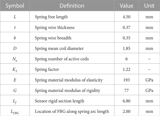
TABLE 1. Sensor parameter definitions and quantitative values.

5.2 Identification of d_r and θ_r

Figure 6A shows the results of the experimental procedure carried out for the identification of d_r and θ_r. The force sensor was rotated about its longitudinal axis within a range of 0–360° at increments of approximately 10°. The hanging weight and other environmental conditions were kept constant throughout the experiment. As expected, the effective curvature κ_eff remained almost constant for all angular configurations, varying with less than 10% of its total magnitude. Figure 6A also clearly shows that the measured strain in the central core ϵ₀ does not remain constant but rather varies sinusoidally with the orientation of the load. As previously shown in (26a), the strain in the central core ϵ₀ is a combination of longitudinal strain ϵ_long and bending due to a geometric offset from the center d_r cos θ_rbκ_eff. The values for ϵ_long, d_r and θ_r were identified through least squares fitting using the data for ϵ₀ and found to be 2 ⋅ 10^–6, 4.1 ⋅ 10^–7 m, and 3.97 rad respectively.

FIGURE 6

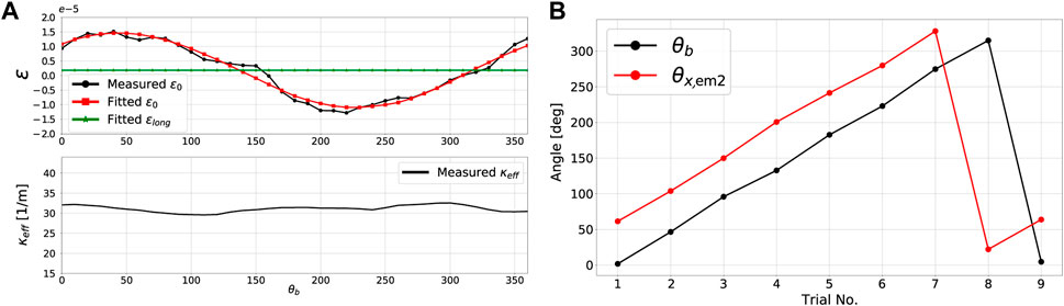
FIGURE 6. Catheter tip force sensor calibration results: (A) central core strain and curvature profiles during the identification of d_r and θ_r, and (B) θ_b and θ_x2 profiles for different force sensor rotational configurations about its longitudinal axis.

5.3 Identification of angles θ_x1 and θ_x2

The procedure for the identification of EM angles θ_x1 and θ_x2 was straightforward as previously outlined in Section 4.4. A 3D line was fitted from position data of EM one during its motion along the constrained 1D slot shown in Figure 5D. Angle θ_x1, which is the angle between the x − axis of EM one and this 3D line, was found to be θ_x1 = 3.96 rad Figure 6B shows the profiles of the bend angle θ_b and the angle of the x − axis of EM 2 with respect to the direction of gravity, θ_x,em2, for different catheter and force sensor rotational configurations. As shown in Figure 6B, it is clear that the difference between the two angles is constant for the different rotational configurations. This difference is the definition of θ_x2 and was found to be around 59.6°.

5.4 Force calibration and resolution

The force calibration procedure involved gathering several data including: 1) FBG wavelength shifts, 2) EM sensor poses, and 3) 3D ground truth forces. Data coming from the different sources were synchronized in time to obtain a data sampling rate of 40 Hz. Note that this limitation in sampling frequency is due to the commercial EM system. The MCF wavelength shifts can be in principle measured at around 250 Hz. The wavelength shifts were used to compute the input measurement vector Θ, while the 3D ground truth forces and EM poses were used to compute the force vector F. Variation of the force vector’s xyz components was obtained by modifying the pose and contact force of the catheter tip force sensor with respect to the Nano17 force sensor. The obtained force ranges for the xyz components of F were 0.40 N, 0.35 N, and 0.51 N respectively. The obtained standard deviation of the applied xyz force components of F were 0.072 N, 0.071 N, and 0.11 N respectively. The calibration data set contained data for a total duration of around 760 s. The calibration matrix C = FΘ⁺ was found to be:

$\mathit{C}=\left[\begin{array}{ccc}\hfill -0.003556\hfill & \hfill 0.000079\hfill & \hfill -0.003682\hfill \\ \hfill 0.000061\hfill & \hfill -0.003932\hfill & \hfill -0.008789\hfill \\ \hfill 0.000003\hfill & \hfill 0.000369\hfill & \hfill -0.749846\hfill \end{array}\right].$

The decoupling of lateral and longitudinal forces with respect to their respective measurements can be clearly seen from the calibration matrix C, but also from the cross-correlation matrix R_cc:

${\mathit{R}}_{\mathit{c}\mathit{c}}=\left[\begin{array}{ccc}\hfill -0.992596\hfill & \hfill 0.262518\hfill & \hfill -0.004549\hfill \\ \hfill 0.255637\hfill & \hfill -0.985295\hfill & \hfill 0.198597\hfill \\ \hfill -0.006603\hfill & \hfill 0.222581\hfill & \hfill -0.986881\hfill \end{array}\right].$

A measurement vector Θ_min based on the minimum wavelength shift Λ_min can be constructed such that ${\mathbf{\Theta }}_{\mathit{min}}=\left[{\kappa }_{\mathit{eff,min}}\right.$, κ_eff,min, ${\left.{\mathrm{\Lambda }}_{\min }\right]}^T$, where κ_eff,min is found through replacing Λ_min into 9) and consequently into (21). The actual force resolution could thus be found from CΘ_min yielding longitudinal and lateral force resolutions of 7.42 ⋅ 10^–3 N and 8.07 ⋅ 10^–4 N, respectively. It can be seen that the actual and theoretical force resolutions are highly comparable, both for the longitudinal and lateral cases. This validates the proposed theoretical sensor design approach and allows for sensor dimensioning based on predetermined performance criteria. Note that in principle, the longitudinal and lateral force resolutions can be made equal by dimensioning the sensor parameters to be constrained such that Ω_long = Ω_lat, i.e., equating expressions (17) and (25). This however, may sometimes not be possible due to additional geometric and manufacturing constraints, as was the case in this work.

5.5 Performance validation

Besides the previously outlined calibration dataset, a separate dataset was measured to validate the sensor’s performance. The data gathering methodology was identical to what has been previously outlined. Synchronized data were again measured at a sampling rate of 40 Hz for an increased total duration of around 1540 s. Figure 7A shows the results of this procedure employing the previously obtained calibration matrix C. Two key observations can be made: 1) the variation of force output follows a clear linear relationship with measurement input, and 2) hysteresis is negligible as the data exhibits a minimum R² value of 0.968 between force output and measurement input. Furthermore, Figure 7B shows the temporal evolution of ground truth and calibrated forces during the data gathering procedure. Table 2 provides a summary of the corresponding force errors between the ground truth and calibrated forces. Longitudinal force estimations remain primarily within a ±0.018 N error range, while lateral force estimations remain primarily within a ±0.010 N error range. The results show that the force estimation accuracy of the developed sensor is either comparable, or superior, to other state of the art force sensors.

FIGURE 7

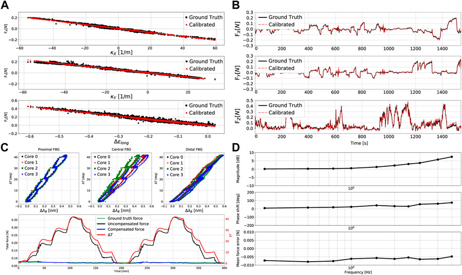
FIGURE 7. Catheter tip force sensor calibration results: (A) relationships between the 3D measured and calibrated forces versus input measurements κ_x, κ_y and Δϵ_long, (B) comparison of the ground truth and estimated 3D forces for different force configurations across time, (C) relationships between temperature change and wavelength shift for the three FBG sets, and comparison of temperature compensated and temperature uncompensated force estimations, (D) dynamic frequency-based force estimation bode plot and mean force error versus frequency.

TABLE 2

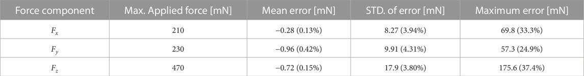
TABLE 2. Validated sensor performance (STD. = standard deviation). Percentages are with respect to the maximum applied forces.

5.6 Temperature compensation

Temperature characterization experiments involved varying the temperature from around 20°C–60°C and back with 10°C steps for two complete cycles. This was initially done with the sensor being free and unloaded in order to characterize the temperature and wavelength shift relationship. The same procedure was then carried out again with a load hanging from the force sensor. Note that the temperature variation was limited to 60°C to protect the catheter and its constituents from permanent damage. The experiment was performed to prove the force sensor’s temperature compensation capability, and is thus expected to operate similarly for higher temperature ranges. The results of these temperature characterization experiments are shown in Figure 7C (top three plots). As predicted, the relationship between temperature change ΔT and wavelength shift Δλ_B is fairly linear for all FBG sets. The minimum R² value amongst these linear relationships was found to be 0.968. Figure 7C also depicts the evolution of temperature across time and illustrates the sensor’s temperature uncompensated and compensated force estimations. It is clear that without temperature compensation, the estimated force drifts far away from the ground truth, resulting in poor sensor performance. On the other hand, incorporating temperature compensation allows for eliminating the effect of temperature on the output force estimation. Temperature compensation maintained force estimation errors within a maximum of ±0.008 N. Hence, it becomes evident that the overall sensor performance is maintained over the wide range of temperature variations.

5.7 Dynamic force behaviour and repeatability

Considering that the force sensor is expected to operate within a dynamic beating heart environment, characterizing its behaviour under such conditions is crucial to asses the force sensor’s performance. Although average human heart motion frequencies range between 1–2 Hz (Chang et al., 2018), the force sensor was subjected to sinusoidal force profiles with frequencies from 0.25 Hz up to 5 Hz to explore its dynamic limits. The results of these dynamic characterization experiments are shown in the bode and error plots of Figure 7D. Sensor gains and phase shifts varied from 0.1–7.4 dB and 8.5–75.1° respectively, for the previously outlined range of frequencies. The mean force error magnitude however, remained almost constant at around 0.006 N. The sensor gain remained under 3 dB for frequencies $\le 2.5$ Hz, with a phase shift of 29° at that point. This means that the system’s operable bandwidth is within the range 0–2.5 Hz with minimal deviation upon the force estimation magnitudes and phase shifts. It is thus clear that the force sensor would be able to operate adequately within the frequency range found within a beating heart.

The force sensor’s repeatability was investigated using the setup for the dynamic loading. Here, an external force with known magnitude was cyclically applied upon the force sensor (at a rate of 0.25 Hz) for a given force range. The resulting linearity of the response, given as the R² value between the ground truth and estimated forces, was found to be R² = 0.953. The sensor’s repeatability, given as the standard deviation of the difference between the ground truth and estimated forces, was found to be 6.24 mN. These results clearly indicate the sensor’s high linearity and repeatable behaviour.

6 Conclusion and future work

This paper presented the design, development, and complete performance validation of a new type of catheter tip force sensor. The sensor’s working principle is based on a helical spring flexure. There are several benefits associated with the use of a helical spring flexural design as compared with other flexural designs, e.g., parallel hinged flexures combined with leaf springs (Gao et al., 2018) or multi-hinged and multi-component flexures (Tang et al., 2022). These include: 1) reduced number of flexural components, 2) simplicity of manufacturing and assembly, 3) simplicity of dimensioning, i.e., scalability, 4) larger flexural axi-symmetry, and 5) design based on known and well-established spring theory. The multi-component flexural design, as proposed in the designs of Gao et al. (2018); Tang et al. (2022), however, does provide the benefit of independent dimensioning and customization of the lateral and longitudinal flexures. In our proposed design, the helical spring flexure is combined with a FBG-inscribed MCF. The MCF is able to measure longitudinal strains which are proportional to the magnitudes of external longitudinal forces. Furthermore, the MCF is also able to measure curvature and it direction which is proportional to the magnitude and direction of external lateral forces. The advantage of using a MCF in the force sensor design not only allows for tip force sensing, but also shape sensing, body force estimation, and temperature monitoring. All of these capabilities can be integrated using one MCF within a single catheter embodiment. This paper further presents an elaborated approach to allow for the easy design and dimensioning of sensor parameters based on predetermined requirements. The approach provides a way to decouple between measurements related to combined longitudinal and lateral forces. Moreover, by using information from two extra unstrained FBG sets, the approach also provides a robust method to compensate for environmental temperature changes, nullifying their effect upon force estimations. An experimental force sensor prototype was constructed, calibrated, and its performance was validated with regards to several key aspects such as: 1) force estimation accuracy, 2) decoupling of longitudinal and lateral forces, 3) input measurement versus output force linearity, 4) temperature compensation performance, and 5) dynamic performance. Targeted future work aspects include: a) design for medical sterilizability, b) inclusion of ablation electrodes and testing during ablation, and c) performing in-vivo animal experiments to study the feasibility of using the force sensor within a realistic environment.

Data availability statement

The original contributions presented in this work are included in the article/supplementary material. Further inquiries can be directed to the corresponding author.

Author contributions

In this work, OA and EVP proposed the research topic as an extension to the state-of-the-art methods for estimation of catheter tip forces. OA conducted the theoretical development, simulations, experiments, data post-processing and analysis, and writing of the manuscript. MO, JV, EL, and EVP provided continuous guidance and feedback regarding the proposed force sensor design and brought about different ideas for the direction of the research. Furthermore, MO, JV, EL, and EVP provided valuable feedback and review of the manuscript.

Funding

This work has received funding from the Flemish Agency of Innovation and Entrepreneurship (VLAIO) under grant number HBC. 2018.2046.

Conflict of interest

The authors declare that the research was conducted in the absence of any commercial or financial relationships that could be construed as a potential conflict of interest.

Publisher’s note

All claims expressed in this article are solely those of the authors and do not necessarily represent those of their affiliated organizations, or those of the publisher, the editors and the reviewers. Any product that may be evaluated in this article, or claim that may be made by its manufacturer, is not guaranteed or endorsed by the publisher.

References

Abushagur, A. A., Arsad, N., Reaz, M. I., and Bakar, A. A. A. (2014). Advances in bio-tactile sensors for minimally invasive surgery using the fibre Bragg grating force sensor technique: A survey. Sensors Switz. 14, 6633–6665. doi:10.3390/s140406633

PubMed Abstract | CrossRef Full Text | Google Scholar

Al-Ahmad, O., Ourak, M., Van Roosbroeck, J., Vlekken, J., and Vander Poorten, E. (2020). Improved FBG-based shape sensing methods for vascular catheterization treatment. IEEE Robotics Automation Lett. 5, 1–4694. doi:10.1109/lra.2020.3003291

CrossRef Full Text | Google Scholar

Al-Ahmad, O., Ourak, M., Vlekken, J., and Vander Poorten, E. (2021). FBG-based estimation of external forces along flexible instrument bodies. Front. Robotics AI 2021, 718033. doi:10.3389/frobt.2021.718033

PubMed Abstract | CrossRef Full Text | Google Scholar

Aloi, V. A., and Rucker, D. C. (2019). Estimating loads along elastic rods. Proc. - IEEE Int. Conf. Robotics Automation 2019, 2867–2873. doi:10.1109/ICRA.2019.8794301

CrossRef Full Text | Google Scholar

Bandari, N., Dargahi, J., and Packirisamy, M. (2020). Tactile sensors for minimally invasive surgery: A review of the state-of-the-art, applications, and perspectives. IEEE Access 8, 7682–7708. doi:10.1109/access.2019.2962636

CrossRef Full Text | Google Scholar

Bourier, F., Gianni, C., Dare, M., Deisenhofer, I., Hessling, G., Reents, T., et al. (2017). Fiberoptic contact-force sensing electrophysiological catheters: How precise is the technology? J. Cardiovasc. Electrophysiol. 28, 109–114. doi:10.1111/jce.13100

PubMed Abstract | CrossRef Full Text | Google Scholar

Bourier, F., Hessling, G., Ammar-Busch, S., Kottmaier, M., Buiatti, A., Grebmer, C., et al. (2016). Electromagnetic contact-force sensing electrophysiological catheters: How accurate is the technology? J. Cardiovasc. Electrophysiol. 27, 347–350. doi:10.1111/jce.12886

PubMed Abstract | CrossRef Full Text | Google Scholar

Calkins, H., Kuck, K. H., Cappato, R., Brugada, J., John Camm, A., Chen, S. A., et al. (2012). 2012 HRS/EHRA/ECAS expert consensus statement on catheter and surgical ablation of atrial fibrillation: Recommendations for patient selection, procedural techniques, patient management and follow-up, definitions, endpoints, and research trial design. J. Interventional Cardiac Electrophysiol. 33, 171–257. doi:10.1007/s10840-012-9672-7

PubMed Abstract | CrossRef Full Text | Google Scholar

Calkins, H., Reynolds, M. R., Spector, P., Sondhi, M., Xu, Y., Martin, A., et al. (2009). Treatment of atrial fibrillation with antiarrhythmic drugs or radiofrequency ablation: Two systematic literature reviews and meta-analyses. Circulation Arrhythmia Electrophysiol. 2, 349–361. doi:10.1161/circep.108.824789

PubMed Abstract | CrossRef Full Text | Google Scholar

Chang, H., Chen, J., and Liu, Y. (2018). Micro-piezoelectric pulse diagnoser and frequency domain analysis of human pulse signals. J. Traditional Chin. Med. Sci. 5, 35–42. doi:10.1016/j.jtcms.2018.02.002

CrossRef Full Text | Google Scholar

Denavit, M. D., Hajjar, J. F., Perea, T., and Leon, R. T. (2018). Elastic flexural rigidity of steel-concrete composite columns. Eng. Struct. 160, 293–303. doi:10.1016/j.engstruct.2018.01.044

CrossRef Full Text | Google Scholar

Gao, A., Zhou, Y., Cao, L., Wang, Z., and Liu, H. (2018). Fiber bragg grating-based triaxial force sensor with parallel flexure hinges. IEEE Trans. Industrial Electron. 65, 8215–8223. doi:10.1109/tie.2018.2798569

CrossRef Full Text | Google Scholar

He, X., Handa, J., Gehlbach, P., Taylor, R., and Iordachita, I. (2014). A submillimetric 3-DOF force sensing instrument with integrated fiber Bragg grating for retinal microsurgery. IEEE Trans. Biomed. Eng. 61, 522–534. doi:10.1109/tbme.2013.2283501

PubMed Abstract | CrossRef Full Text | Google Scholar

Lairikyengbam, S. K., Anderson, M. H., and Davies, A. G. (2003). Present treatment options for atrial fibrillation. Postgrad. Med. J. 79, 67–73. doi:10.1136/pmj.79.928.67

PubMed Abstract | CrossRef Full Text | Google Scholar

Li, H., Song, X., Liang, Y., Bai, X., Liu-Huo, W. S., Tang, C., et al. (2022). Global, regional, and national burden of disease study of atrial fibrillation/flutter, 1990–2019: Results from a global burden of disease study, 2019. BMC Public Health 22, 2015. doi:10.1186/s12889-022-14403-2

PubMed Abstract | CrossRef Full Text | Google Scholar

Li, T., Pan, A., and Ren, H. (2020). A high-resolution triaxial catheter tip force sensor with miniature flexure and suspended optical fibers. IEEE Trans. Industrial Electron. 67, 5101–5111. doi:10.1109/tie.2019.2926052

CrossRef Full Text | Google Scholar

Liang, Q., Zou, K., Long, J., Jin, J., Zhang, D., Coppola, G., et al. (2018). Multi-component FBG-based force sensing systems by comparison with other sensing technologies: A review. IEEE Sensors J. 18, 7345–7357. doi:10.1109/jsen.2018.2861014

CrossRef Full Text | Google Scholar

Moore, J. P., and Rogge, M. D. (2012). Shape sensing using multi-core fiber optic cable and parametric curve solutions. Opt. Express 20, 2967–2973. doi:10.1364/oe.20.002967

PubMed Abstract | CrossRef Full Text | Google Scholar

Noh, Y., Liu, H., Sareh, S., Chathuranga, D. S., Wurdemann, H., Rhode, K., et al. (2016). Image-based optical miniaturized three-axis force sensor for cardiac catheterization. IEEE Sensors J. 16, 7924–7932. doi:10.1109/jsen.2016.2600671

CrossRef Full Text | Google Scholar

Othman, W., Lai, Z. H. A., Abril, C., Barajas-Gamboa, J. S., Corcelles, R., Kroh, M., et al. (2022). Tactile sensing for minimally invasive surgery: Conventional methods and potential emerging tactile technologies. Front. Robotics AI 8, 705662. doi:10.3389/frobt.2021.705662

CrossRef Full Text | Google Scholar

Polygerinos, P., Seneviratne, L. D., Razavi, R., Schaeffter, T., and Althoefer, K. (2013). Triaxial catheter-tip force sensor for MRI-guided cardiac procedures. IEEE/ASME Trans. Mechatronics 18, 386–396. doi:10.1109/tmech.2011.2181405

CrossRef Full Text | Google Scholar

Polygerinos, P., Zbyszewski, D., Schaeffter, T., Razavi, R., Seneviratne, L. D., and Althoefer, K. (2010). MRI-compatible fiber-optic force sensors for catheterization procedures. IEEE Sensors J. 10, 1598–1608. doi:10.1109/jsen.2010.2043732

CrossRef Full Text | Google Scholar

Roth, G. A., Mensah, G. A., Johnson, C. O., Addolorato, G., Ammirati, E., Baddour, L. M., et al. (2020). Global burden of cardiovascular diseases and risk factors, 1990-2019: Update from the GBD 2019 study. J. Am. Coll. Cardiol. 76, 2982–3021. doi:10.1016/j.jacc.2020.11.010

PubMed Abstract | CrossRef Full Text | Google Scholar

Shi, C., Li, T., and Ren, H. (2018). A millinewton resolution fiber bragg grating-based catheter two-dimensional distal force sensor for cardiac catheterization. IEEE Sensors J. 18, 1539–1546. doi:10.1109/jsen.2017.2779153

CrossRef Full Text | Google Scholar

Shi, C., Luo, X., Qi, P., Li, T., Song, S., Najdovski, Z., et al. (2017). Shape sensing techniques for continuum robots in minimally invasive surgery: A survey. IEEE Trans. Biomed. Eng. 64, 1665–1678. doi:10.1109/tbme.2016.2622361

PubMed Abstract | CrossRef Full Text | Google Scholar

Shin, D., Kim, T., and Kim, H. U. (2018). “Development of tri-axial fiber bragg grating force sensor in catheter application,” in MeMeA-2018 IEEE International Symposium on Medical Measurements and Applications, Proceedings, Rome, Italy, 11-13 June 2018 (IEEE), 1–5. doi:10.1109/MeMeA.2018.8438714

CrossRef Full Text | Google Scholar

Song, Y., Guo, S., Yin, X., Zhang, L., Hirata, H., Ishihara, H., et al. (2018). Performance evaluation of a robot-assisted catheter operating system with haptic feedback. Biomed. Microdevices 20, 294. doi:10.1007/s10544-018-0294-4

PubMed Abstract | CrossRef Full Text | Google Scholar

Sra, J. (2008). Atrial fibrillation ablation complications. J. Interventional Cardiac Electrophysiol. 22, 167–172. doi:10.1007/s10840-007-9200-3

PubMed Abstract | CrossRef Full Text | Google Scholar

Srimathveeravalli, G., Kesavadas, T., and Li, X. (2010). Design and fabrication of a robotic mechanism for remote steering and positioning of interventional devices. Int. J. Med. Robotics Comput. Assisted Surg. 6, 160–170. doi:10.1002/rcs.301

PubMed Abstract | CrossRef Full Text | Google Scholar

Su, H., Iordachita, I. I., Tokuda, J., Hata, N., Liu, X., Seifabadi, R., et al. (2017). Fiber-Optic force sensors for MRI-guided interventions and rehabilitation: A review. IEEE Sensors J. 17, 1952–1963. doi:10.1109/jsen.2017.2654489

PubMed Abstract | CrossRef Full Text | Google Scholar

Taffoni, F., Formica, D., Saccomandi, P., Di Pino, G., and Schena, E. (2013). Optical fiber-based MR-compatible sensors for medical applications: An overview. Sensors (Basel) 13, 14105–14120. doi:10.3390/s131014105

PubMed Abstract | CrossRef Full Text | Google Scholar

Tang, B., Lv, W., Zhang, W., Ye, Y., Li, Y., Zhou, Q., et al. (2017). Impact of contact force technology on reducing the recurrence and major complications of atrial fibrillation ablation: A systematic review and meta-analysis. Anatol. J. Cardiol. 17, 82–91. doi:10.14744/anatoljcardiol.2016.7512

PubMed Abstract | CrossRef Full Text | Google Scholar

Tang, Z., Wang, S., Li, M., and Shi, C. (2022). Development of a distal tri-axial force sensor for minimally invasive surgical palpation. IEEE Trans. Med. Robotics Bionics 4, 145–155. doi:10.1109/tmrb.2022.3142361

CrossRef Full Text | Google Scholar

Wahl, A. (1944). Mechanical springs. Chennai: Penton Publishing Company.

Google Scholar

Zhou, X., Lv, W., Zhang, W., Ye, Y., Li, Y., Zhou, Q., et al. (2017). Impact of contact force technology on reducing the recurrence and major complications of atrial fibrillation ablation: A systematic review and meta-analysis. Anatol. J. Cardiol. 17, 82–91. doi:10.14744/AnatolJCardiol.2016.7512

PubMed Abstract | CrossRef Full Text | Google Scholar