Connection between single-layer quantum approximate optimization algorithm interferometry and thermal distribution sampling

1 Introduction

Variational quantum algorithms (VQAs) are a promising framework for solving computationally hard tasks (Cerezo et al., 2021; Bharti et al., 2022). These algorithms are based on a quantum circuit with tunable parameters acting as an ansatz. Finding the minimum energy state among a discrete set of possible solutions (combinatorial optimization problems) (Nemhauser and Wolsey, 1988; Moll et al., 2018) and drawing samples from a classical probability distribution (sampling problems) (Lund et al., 2017; Wild et al., 2021) are two examples of worthwhile challenges addressed in this framework.

Among the plethora of proposed VQAs, the quantum approximate optimization algorithm (QAOA) (Farhi et al., 2014) has received special attention from the scientific community, with remarkable empirical and theoretical results on the algorithm’s performance (Harrigan et al., 2021; Farhi et al., 2022; Blekos et al., 2023). The ansatz of the QAOA is inspired by a Trotterized adiabatic evolution capable of approximating the minimum energy state of a given cost function. An advantage of the practical implementation of the QAOA is that the number of variational parameters in the quantum circuit to be optimized is independent of the problem size; in contrast, the depth of the circuit increases with the quality of the approximation of the fundamental state.

Beyond its original use in approximating ground states, the QAOA has recently demonstrated utility from a global sampling perspective (Farhi and Harrow, 2019). It has been shown that the shallowest version of the algorithm produces a probability distribution that cannot be simulated by classical computation because otherwise, the polynomial hierarchy would collapse. Therefore, sampling the QAOA circuit in some variational parameter ranges could exhibit quantum supremacy (Preskill, 2018), which is understood as a task that can be more efficiently done using a quantum computer than a classical one. This result is connected to previous demonstrations of the hardness of simulating quantum circuits, for instance, Boson sampling (Brod, 2015) or instantaneous quantum polynomial time (IQP) circuits (Bremner et al., 2010, 2016).

Despite the importance of this theoretical result, it gives no clue about the nature of the probability distribution generated by the QAOA, nor whether sampling from it has any practical interest beyond combinatorial optimization or a quantum supremacy demonstration. Following this direction, we studied the global structure and probability distribution in the energy space of the single-layer QAOA ansatz in Díez-Valle et al. (2023). In that letter, we provide evidence for a clear connection between the QAOA and thermal distribution sampling with probability amplitude distributions resembling Boltzmann distributions at low temperatures. We call such distributions QAOA pseudo-Boltzmann states. The excellent performance of QAOA revealed at temperatures below the state-of-the-art theoretical limit to fast mixing of Markov Chain Monte Carlo methods (Eldan et al., 2021).

In the current manuscript, we expand the theoretical derivation of pure thermal-like QAOA states introduced in Díez-Valle et al. (2023). More specifically, we extend the discussion of single-layer QAOA amplitudes by portraying the algorithm as an energy interferometer and providing details on the mathematical derivation of the pseudo-Boltzmann states. We also provide further justification for the assumption of normality in the internal spin model correlations, extend the study of the evolution of the probability distribution with the mixing angle, and shed more light on the implications of these results.

The paper is structured as follows: first, in Section 2, we review the main ingredients of the quantum approximate optimization algorithm and introduce an intuitive picture of the QAOA as an interferometer in energy space. In Section 3.1, we extend the interferometric picture to the multilayer scenario and derive the analytical amplitudes of the final wave function. In Section 3.2, we specify the results of the previous section to the case where an Ising model Hamiltonian defines the cost function. We detail the internal correlations between the eigenstates of the Hamiltonian in degenerate and non-degenerate scenarios, leading to a closed expression for the probability amplitudes of the QAOA wavefunction. We connect such probability amplitudes to the sampling of Boltzmann or thermal-like distributions in Section 4 and also analyze the features that these results reveal about the distribution behavior as we change the variational parameters of the algorithm. We conclude with a perspective on the importance of the pseudo-Boltzmann QAOA states and approximate thermal sampling in Section 5.

2 Interferometric interpretation of the QAOA

2.1 The quantum approximate optimization algorithm

The QAOA aims to find good approximate solutions to combinatorial optimization problems (Farhi et al., 2014) that are defined by a classical objective function E(x) mapping N-binary strings to real values:

$E\left(\mathbf{x}\right):{\left\{\mathrm{0,1}\right\}}^N\to \mathbb{R}.(1)$

The algorithm’s goal is to find a binary string x* that minimizes the function E_min ≡ min_xE(x), or at least that achieves a good approximation ratio r ∈ [0, 1].

$\frac{{\max }_{\mathbf{x}}E\left(\mathbf{x}\right)-E\left(\mathbf{x}\right)}{{\max }_{\mathbf{x}}E\left(\mathbf{x}\right)-{\min }_{\mathbf{x}}E\left(\mathbf{x}\right)}\ge r.(2)$

This optimization problem is equivalent to finding the ground state of a spin Hamiltonian $\widehat{E}$, where each binary variable x_i describes the state of one spin ${\sigma }_i^z$ as $\mathbf{x}\to \frac{1}{2}(1+{\mathit{\sigma }}^z)$:

${\widehat{E}}_{\mathit{min}}\equiv {\min }_{{\mathit{\sigma }}^z}\langle {\mathit{\sigma }}^z|\widehat{E}\left({\mathit{\sigma }}^z\right)|{\mathit{\sigma }}^z\rangle ={\min }_{\mathbf{x}}\langle \mathbf{x}|\widehat{E}\left(\mathbf{x}\right)|\mathbf{x}\rangle .(3)$

A well-known approach to solving these problems is the quantum adiabatic algorithm (QAA), which ensures the achievement of the global minimum given a sufficiently long run time T (Farhi et al., 2000; Farhi et al., 2001). The adiabatic protocol is guided by a time-dependent Hamiltonian, such as

${\widehat{H}}_{\text{QAA}}\left(t\right)=-\left[\left(1-f\left(\frac{t}{T}\right)\right){\widehat{H}}_x+f\left(\frac{t}{T}\right)\widehat{E}\right],(4)$

where ${\widehat{H}}_x={\sum }_i^N{\sigma }_i^x$ with ${\sigma }_i^x$ being the Pauli operator acting on the ith qubit and f(x) is the schedule function with f(0) = 0 and f(1) = 1. The adiabatic theorem guarantees that a sufficiently slow time evolution will keep the system in its ground state. Thus, an evolution that starts with the ground state of ${\widehat{H}}_x$,

$|\mathrm{\Psi }\left(0\right)\rangle =\frac{1}{\sqrt{2^N}}{\displaystyle \sum _{\mathbf{x}}}|\mathbf{x}\rangle \equiv |{+\rangle }^{\otimes N},(5)$

will approximately bring the system to the ground state of $\widehat{E}$,

$|\mathrm{\Psi }\left(T\right)\rangle =|{\mathbf{x}}_{\mathit{min}}\rangle .(6)$

To ensure success, the runtime T must scale as $T=O\left({\mathrm{\Delta }}_{\text{min}}^{-2}\right)$, where Δ_min is the minimum spectral gap (Albash and Lidar, 2018). The QAOA proposes a Trotterized approximation to adiabatic evolution consisting of a quantum circuit built by the alternation of the following two operators:

$|{\mathrm{\Psi }}_{\text{QAOA}-\text{p}}\left(\mathit{\gamma },\mathit{\theta }\right)\rangle =U\left({\widehat{H}}_x,{\theta }_p\right)U\left(\widehat{E},{\gamma }_p\right)\dots U\left({\widehat{H}}_x,{\theta }_2\right)U\left(\widehat{E},{\gamma }_2\right)U\left({\widehat{H}}_x,{\theta }_1\right)U\left(\widehat{E},{\gamma }_1\right)H^{\otimes N}|{0\rangle }^{\otimes N},(7)$

with H denoting single-qubit Hadamard gates, and

$U\left(\widehat{E},\gamma \right)=e^{-i\gamma \widehat{E}},(8)$

$U\left({\widehat{H}}_x,\theta \right)=e^{-i\theta {\widehat{H}}_x}=\prod _j^N{e}^{-i\theta {\sigma }_j^x}\equiv R_x{\left(\theta \right)}^{\otimes N},(9)$

where γ = (γ₁, γ₂, …, γ_p) and θ = (θ₁, θ₂, …, θ_p) are set of variational angles that can be tuned to approximate the ground state of the cost Hamiltonian $\widehat{E}$ and p is the number of layers that determines the depth of the quantum circuit and the accuracy of the algorithm. The infinite depth limit p → ∞ returns the adiabatic evolution, showing that we can get a good enough approximation to the minimum of the optimization problem for sufficiently large p.

2.2 The QAOA as an interferometer in energy space

Let us highlight the QAOA’s potential in small-depth regimes by introducing an interpretation of the QAOA’s circuit as an interferometer operating globally in energy space. We will derive analytical results for the interference amplitude in later sections, focusing on the p = 1 single-layer ansatz (see Eq. 7):

$|{\mathrm{\Psi }}_{\text{QAOA}-1}\left(\gamma ,\theta \right)\rangle =R_x{\left(\theta \right)}^{\otimes N}{e}^{-i\gamma \widehat{E}}{H}^{\otimes N}|{0\rangle }^{\otimes N}.(10)$

As sketched in Figure 1, the Hadamard gate splits the quantum state |0⟩ into a superposition of all states in the computational basis, acting like a multidimensional “mirror”:

$|s_1\rangle =|{+\rangle }^{\otimes N}=\frac{1}{\sqrt{2^N}}{\displaystyle \sum _{\mathbf{x}}}|\mathbf{x}\rangle .(11)$

Then, the evolution with the diagonal cost Hamiltonian $\widehat{E}|\mathbf{x}\rangle =E_{\mathbf{x}}|\mathbf{x}\rangle$, given by the operator $U_E(\widehat{E},\gamma )$, imparts phases on all states, acting like the branches of the interferometer:

$|s_2\rangle =e^{-i\gamma \widehat{E}}|s_1\rangle =\frac{1}{\sqrt{2^N}}{\displaystyle \sum _{\mathbf{x}}}{e}^{-i\gamma E_{\mathbf{x}}}|\mathbf{x}\rangle .(12)$

Finally, the mixing operator R_x(θ)^⊗N recombines the energy states so that the interference transforms the energy-dependent relative phases in measurable probability amplitudes:

$|{\mathrm{\Psi }}_{\text{QAOA}-1}\left(\gamma ,\theta \right)\rangle =R_x{\left(\theta \right)}^{\otimes N}|s_2\rangle ={\displaystyle \sum _{\mathbf{x}}}{F}_{\mathbf{x}}\left(E_{\mathbf{x}},\gamma ,\theta \right)|\mathbf{x}\rangle .(13)$

FIGURE 1

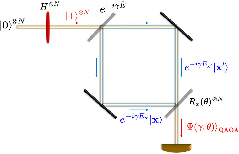
FIGURE 1. Interferometric interpretation of the quantum approximate optimization algorithm circuit.

This intuition is much clearer when looking at the algorithm operating on a single qubit, with rotation R_x(θ):

$R_x\left(\theta \right)=e^{-i\theta {\sigma }^x}=\mathbb{I}\cos \theta -i{\sigma }^x\sin \theta =\left(\begin{array}{cc}\hfill \cos \theta \hfill & \hfill -i\sin \theta \hfill \\ \hfill -i\sin \theta \hfill & \hfill \cos \theta \hfill \end{array}\right).(14)$

Consider the following two-state subspace:

$\left\{|{\mathbf{x}}_0\rangle =|0,x_1,x_2,\dots ,x_N\rangle ,|{\mathbf{x}}_1\rangle =|1,x_1,x_2,\dots ,x_N\rangle \right\},$

where x_i = {0, 1} (so x₀ and x₁ differ by only 1 bit), with energies $E_{{\mathbf{x}}_0}\equiv \langle {\mathbf{x}}_0|\widehat{E}|{\mathbf{x}}_0\rangle$ and $E_{{\mathbf{x}}_1}\equiv \langle {\mathbf{x}}_1|\widehat{E}|{\mathbf{x}}_1\rangle$. The probability amplitudes before the local interference are

$A_{{\mathbf{x}}_0}^2=|⟨{\mathbf{x}}_0|s_2⟩{|}^2,A_{{\mathbf{x}}_1}^2=|⟨{\mathbf{x}}_1|s_2⟩{|}^2,(15)$

respectively. After applying the local gate in Eq. 14 on the qubit that corresponds to the different bit, the interference shifts the amplitudes to $N_{{\mathbf{x}}_0}$ and $N_{{\mathbf{x}}_1}$:

$\left(\begin{array}{c}\hfill N_{{\mathbf{x}}_0}\hfill \\ \hfill N_{{\mathbf{x}}_1}\hfill \end{array}\right)=R_x\left(\theta \right)\left(\begin{array}{c}\hfill e^{-i\gamma E_{{\mathbf{x}}_0}}{A}_{{\mathbf{x}}_0}\hfill \\ \hfill e^{-i\gamma E_{{\mathbf{x}}_1}}{A}_{{\mathbf{x}}_1}\hfill \end{array}\right)=e^{-i\gamma E_{{\mathbf{x}}_0}}\left(\begin{array}{c}\hfill A_{{\mathbf{x}}_0}\cos \theta -i{A}_{{\mathbf{x}}_1}{e}^{-i\gamma F_{{\mathbf{x}}_1,{\mathbf{x}}_0}}\sin \theta \hfill \\ \hfill -i{A}_{{\mathbf{x}}_0}\sin \theta +A_{{\mathbf{x}}_1}{e}^{-i\gamma F_{{\mathbf{x}}_1,{\mathbf{x}}_0}}\cos \theta \hfill \end{array}\right),(16)$

where $F_{{\mathbf{x}}_1,{\mathbf{x}}_0}\equiv E_{{\mathbf{x}}_1}-E_{{\mathbf{x}}_0}$. Thus, the probability amplitudes become

$\begin{array}{ll}\hfill N_0^2=& A_{{\mathbf{x}}_0}^2{\cos }^2\theta +A_{{\mathbf{x}}_1}^2{\sin }^2\theta -A_{{\mathbf{x}}_0}{A}_{{\mathbf{x}}_1}\sin \left(2\theta \right)\sin \left(\gamma F_{{\mathbf{x}}_1,{\mathbf{x}}_0}\right)\hfill \\ \hfill N_1^2=& A_{{\mathbf{x}}_0}^2{\sin }^2\theta +A_{{\mathbf{x}}_1}^2{\cos }^2\theta +A_{{\mathbf{x}}_0}{A}_{{\mathbf{x}}_1}\sin \left(2\theta \right)\sin \left(\gamma F_{{\mathbf{x}}_1,{\mathbf{x}}_0}\right).\hfill \end{array}(17)$

Note that the relative phase between the states $\gamma F_{{\mathbf{x}}_1,{\mathbf{x}}_0}=\gamma \left(E_{{\mathbf{x}}_1}-E_{{\mathbf{x}}_0}\right)$ controls the amplification. Therefore, assuming $\sin \left(2\theta \right)<0$ and γ > 0 or vice versa and provided the angle γ is sufficiently small, the interference term always increases the population of the lowest energy state and reduces that of the other. Furthermore, Eq. 17 also reflects how the relative sign between $\sin \left(2\theta \right)$ and γ controls the direction of optimization. The probability amplitude of the lowest/highest energy state is enhanced when the signs are opposite/equal.

This interferometric behavior expanded to the N-level scenario imposes non-trivial, structure-dependent upper bounds on the |θ| and |γ| angles to avoid symmetries and random scrambling of the energy states. In particular, Eq. 17 shows that for the single-qubit interference:

$n\pi \le \theta <\left(n+1\right)\pi \mathrm{a}\mathrm{n}\mathrm{d}|\gamma |<\frac{\pi }{F_{{\mathbf{x}}_{\mathit{max}},{\mathbf{x}}_{\mathit{min}}}}\sim O\left(\Vert \widehat{E}{\Vert }^{-1}\right),(18)$

with $n\in \mathbb{Z}$. The N-qubit interference makes this picture richer and more complicated, as derived in the next sections. Analytical and numerical results for the single-layer QAOA on general Ising spin models show that the optimal |γ| for an N-qubit system actually scales as $O(N{\left(N|e|\right)}^{-1/2})$ (Ozaeta et al., 2022; Díez-Valle et al., 2023), where |e| is the number of edges or non-null elements in the coupling matrix J (see Eq. 27). For instance, in the two-level system $\widehat{E}=\frac{1}{2}\mathrm{\Delta }{\sigma }^z$, the probability of measuring the ground state |σ^z = −1⟩ and the highest energy state |σ^z = +1⟩ is

$|⟨{\sigma }^z=\pm 1|\mathrm{\Psi }\left(\gamma ,\theta \right)⟩{|}^2=\frac{1}{2}\left(1+{\sigma }^z\sin \left(2\theta \right)\sin \left(\gamma \mathrm{\Delta }\right)\right),(19)$

which is maximal with optimal angles $\theta =\pm \frac{\pi }{4}$ and $\gamma =\frac{\pi }{2\mathrm{\Delta }}$ (see Figure 2).

FIGURE 2

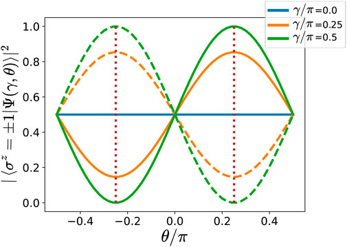
FIGURE 2. Quantum approximate optimization algorithm interferometry on the two-level spin system defined by the Hamiltonian $\widehat{E}=\frac{1}{2}\mathrm{\Delta }{\sigma }^z$ with Δ = 1. We plot the probability amplitude of the ground state σ^z = −1 (dashed lines) and the highest energy state σ^z = +1 (solid lines) for different values of the QAOA angles θ and γ. We highlight the points of maximum amplification, θ = ±π/4 and γ = π/2, with dotted brown lines.

3 Multi-level interferometer amplitude

3.1 General scenario

Let us extend the two-level picture to a general framework dealing with the complete interference spectrum of a single-layer QAOA circuit. We focus on how the QAOA transforms the wavefunction amplitudes:

$F\left(\mathbf{x}\right)\equiv ⟨\mathbf{x}|{\mathrm{\Psi }}_{\text{QAOA}-1}\left(\gamma ,\theta \right)⟩,(20)$

where x is any eigenstate in the energy spectrum that we will denote as the reference state. As previously shown, a local R_x rotation acting on the ith qubit mixes the amplitude between each state x with the corresponding state x′ that differs only on the value of the ith bit (see Eq. 17). Thus, the action of the whole mixing operator $R_x^{\otimes N}$ is that of a complete mixing between all states in the computational basis:

$F\left(\mathbf{x}\right)={\displaystyle \sum _{{\mathbf{x}}^{\prime }}}\frac{e^{-i\gamma E_{{\mathbf{x}}^{\prime }}}}{2^{N/2}}\langle \mathbf{x}|\prod _j^N\left(\cos \theta -i{\sigma }_j^x\sin \theta \right)|{\mathbf{x}}^{\prime }\rangle .(21)$

The weight of each mixing process depends on the number of bits that must be flipped to go from one state x to the other x′, that is, the Hamming distance between both states, and also on the oscillating terms induced by the angles θ and γ. The amplitude of the state generated by the algorithm after the mixing operator $U({\widehat{H}}_x,\theta )$ is given by an interference formula,

$F\left(\mathbf{x}\right)\equiv ⟨\mathbf{x}|\tilde{\mathrm{\Psi }}⟩=\frac{1}{2^{N/2}}{\displaystyle \sum _{{\mathbf{x}}^{\prime }}}\cos {\left(\theta \right)}^{N-H_{\mathbf{x},{\mathbf{x}}^{\prime }}}{\left[-i\sin \left(\theta \right)\right]}^{H_{\mathbf{x},{\mathbf{x}}^{\prime }}}{e}^{-i\gamma E_{{\mathbf{x}}^{\prime }}}(22)$

where $H_{\mathbf{x},{\mathbf{x}}^{\prime }}$ is the Hamming distance between two bit configurations x and x′ that represent the eigenstates of a spin model with energy E_x and $E_{{\mathbf{x}}^{\prime }}$. We can unify the weight sum terms into a single exponential by the following change of variables in which the rotation angle θ is reparameterized in terms of an exponent r and a normalization R,

$\cos \left(\theta \right)=R^{\frac{1}{2}}\exp \left[\frac{r}{2}\right],\sin \left(\theta \right)=R^{\frac{1}{2}}\exp \left[-\frac{r}{2}\right],(23)$

where, due to the symmetries of the interference, we consider $\theta \in (0,\frac{\pi }{2})$ without loss of generality. The sign of γ allows us to define if the interference increases the population of lower or higher energy states so that we cover all the possibilities. By this transformation, the interference amplitudes in Eq. 22 become a sum of exponentials over the entire configuration space,

$F\left(\mathbf{x}\right)={\left(\frac{R\exp \left[r\right]}{2}\right)}^{\frac{N}{2}}{\displaystyle \sum _{{\mathbf{x}}^{\prime }}}\exp \left[-H_{\mathbf{x}{\mathbf{x}}^{\prime }}\left(i\frac{\pi }{2}+r\right)-i\gamma E_{{\mathbf{x}}^{\prime }}\right].(24)$

Because Eq. 24 encompasses all eigenstates of the system encoded in its energy $E_{{\mathbf{x}}^{\prime }}$ and Hamming distance $H_{\mathbf{x},{\mathbf{x}}^{\prime }}$ with the reference state x, it is convenient to introduce a probability distribution relating distances in the computational base to the energy spectrum,

$p\left(H,E;\mathbf{x}\right)=\frac{1}{2^N}{\displaystyle \sum _{{\mathbf{x}}^{\prime }}}\delta \left(H-H_{{\mathbf{xx}}^{\prime }}\right)\delta \left(E-E_{{\mathbf{x}}^{\prime }}\right),(25)$

This expression represents the relative number of eigenstates that, given a reference state x, have a Hamming distance H to that state and energy equal to E. In other words, this distribution captures the internal correlations inherent to the specific spin model. With this definition at hand, we can express the previous sum in Eq. 24 as the average over this probability distribution:

$F\left(\mathbf{x}\right)\propto {\left(\exp \left[r\right]\right)}^{\frac{N}{2}}{\iint }_{-\infty }^{\infty }\exp \left[-H\left(i\frac{\pi }{2}+r\right)-i\gamma E\right]p\left(H,E;\mathbf{x}\right)dHdE.(26)$

Hence, the interference amplitude in Eq. 20 depends on the structure of the energy levels of the spin system manifested in the probability distribution p(H, E; x). In the following sections, we study such a structure to derive a unified expression of the QAOA probability amplitudes for universal Ising spin models.

3.2 Ising models

Next, we focus on a universal set of non-deterministic polynomial time hard (NP-hard) Ising models (Barahona, 1982) and derive this scenario’s interference probability amplitude formula.

A broad spectrum of combinatorial optimization problems can be represented as a spin model described by an Ising Hamiltonian (Lucas, 2014),

$E_I\left(\mathbf{s}\right)=\frac{1}{2}{\displaystyle \sum _{i,j=1}^N}{s}_i{J}_{ij}{s}_j+{\displaystyle \sum _{i=1}^N}{h}_i{s}_i,(27)$

where s = {−1,+1}^N, N is the number of variables, J is an N-by-N square coupling matrix, and the magnetic field h is a vector of N coefficients. The quantum version of this Hamiltonian ${\widehat{E}}_I({\mathit{\sigma }}^{\mathit{z}})$ is simply obtained by replacing the spin variables s with the corresponding Pauli-Z matrices σ^z. The coupling matrix defines a structure in the problem that can be represented by a weighted graph with N vertices, connected by undirected edges i ↔ j that have associated weights J_ij, J_ji. In this work, we study families of models in which the J_ij coefficients are randomly drawn from a normal distribution N(μ = 0, σ²).

This structure, together with the magnetic field values, defines families of optimization problems with different inner correlations and degeneracies. In the following subsections, we derive the interference amplitude for two scenarios that involve distinct energy level structures due to intrinsic global symmetries in the model. These differences necessitate a separate study of each case. Nevertheless, as explained below, the slightly different behaviors of these models converge to a common expression of the QAOA probability amplitude distribution |F(x)|² in Eq. 20. The two scenarios are represented by two well-known combinatorial optimization problems: quadratic unconstrained binary optimization (QUBO) (Kochenberger and Glover, 2004; Kochenberger and Hao, 2014), with a non-degenerate energy spectrum, and the maximum cut (MaxCut) (Nannicini, 2019; Sung et al., 2020; Harrigan et al., 2021), which exhibits a global ${\mathbb{Z}}_2$ symmetry.

3.2.1 Non-degenerate Ising models

The family of QUBO problems is composed of NP-hard binary combinatorial optimization problems with the following associated cost function:

$E_{\text{QUBO}}\left(\mathbf{x}\right)=2{\displaystyle \sum _{i,j}}{x}_i{Q}_{ij}{x}_j,(28)$

where x ∈ {0,1}^N, and Q is an N-by-N square matrix. The mapping of Eq. 28 to the Ising Hamiltonian in Eq. 27, $\mathbf{x}=\frac{1}{2}(1+\mathbf{s})$, leads to

${\tilde{E}}_{\text{QUBO}}=2{\displaystyle \sum _{i,j}}{x}_i{Q}_{ij}{x}_j-{\displaystyle \sum _{i,j}}\frac{1}{2}{Q}_{i,j}=\frac{1}{2}{\displaystyle \sum _{i,j=1}^N}{s}_i{J}_{ij}{s}_j+{\displaystyle \sum _{i=1}^N}{h}_i{s}_i,(29)$

where J = Q and h_j = ∑_i(Q_ij + Q_ji)/2. We consider Q matrices where the non-zero coefficients are randomly drawn from a standard normal distribution N(μ = 0, σ² = 1). Note that the optimization of the function in Eq. 29 is then equivalent to that of Eq. 28.

The cost function in Eq. 29 exhibits no global symmetries. In such non-degenerate situations, the eigenstates appear to be ordered from low to excited states, developing a unique probability distribution p(H, E; x) that is centered at the center of the spectrum and shows a remarkable correlation between $H_{{\mathbf{xx}}^{\prime }}$ and $E_{{\mathbf{x}}^{\prime }}$. Such behavior can be observed in Figure 3. Here, we plot the distribution in the Hamming distance-energy plane of 25,000 samples drawn from a continuous approximation to p(H, E; x) of a single instance of QUBO. Specifically, we first estimate the continuous probability density function by a kernel density estimation (KDE) on the actual discrete instance data (all $H_{{\mathbf{xx}}^{\prime }}$ and $E_{{\mathbf{x}}^{\prime }}$ pairs). Then, we sample from such density function to obtain the plotted distributions. We also perform a fitting of the final distribution to a Gaussian mixture of one or two Gaussians using variational inference and plot the corresponding confidence ellipsoid. This fit was obtained with the BayesianGaussianMixture method of the Python package scikit-learn (Pedregosa et al., 2011). We show the result for x being the ground state (a) and the highest energy state (c). For the sake of clarity, let us consider the upper-left plot, which illustrates the probability distribution p(H, E; x) for the reference state x as the ground state. All alternative states x′ possess higher energy values than E_x. The difference $E_{{\mathbf{x}}^{\prime }}-E_{\mathbf{x}}$ shows a potential correlation with the number of spin flips required to transition from x to x′, that is, the Hamming distance $H_{{\mathbf{xx}}^{\prime }}$. This positive correlation is evident through the presence of a Gaussian function oriented along a diagonal. In contrast, opting for x as the highest energy state (bottom-left plot) reveals an opposite trend: the greater the number of spin flips, the lower the energy level. The Gaussian orientation depends on the covariance between H and E,

${\sigma }_{EH}=\frac{1}{2^N}{\displaystyle \sum _{{\mathbf{x}}^{\prime }}}\left(H_{\mathbf{x}{\mathbf{x}}^{\prime }}-\mathbb{E}\left[H\right]\right)\left(E_{{\mathbf{x}}^{\prime }}-\mathbb{E}\left[E\right]\right),(30)$

which is highly correlated with the energy of the reference state E_x, as shown in Figure 4 of Díez-Valle et al. (2023). In Eq. 30, $\mathbb{E}[\cdot ]$ denotes the expected value of the variable.

FIGURE 3

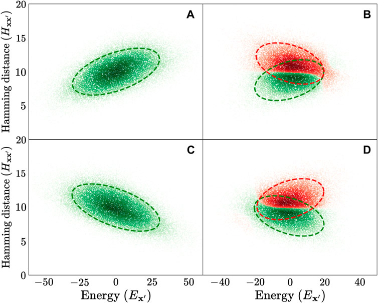
FIGURE 3. Continuous approximation to the probability distribution p(H, E; x) estimated by 25,000 samples drawn from a kernel density estimation (KDE) on a single instance of a non-degenerate problem (A,C) and of a degenerate problem (B,D). We plot the extreme cases when the reference state x is the ground state (A,B) and the highest energy state (C,D). We also fit the obtained distribution to a Gaussian mixture of one (A,C) or two (B,D) bivariate Gaussians, showing the clustering of the samples and the confidence ellipsoid over the distributions.

FIGURE 4

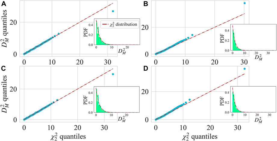
FIGURE 4. Multivariate normality test to show that the structure of the energy levels of the Ising models studied resembles probability distributions p(H, E; x) that can be defined by one or two continuous bivariate Gaussians. We plot the results for 1,000 14-qubit random instances of QUBO (A,C) and MaxCut (B,D) when the reference state x is the ground state (A,B) and the highest energy state (C,D). For each instance of the problem, we calculated the Mahalanobis distances, D_M, of all $(H_{\mathbf{x}{\mathbf{x}}^{\prime }},E_{{\mathbf{x}}^{\prime }})$ samples and display the results of the obtained distributions. If such samples are compatible with a set of samples drawn from a bivariate Gaussian, the obtained Mahalanobis distances must follow the ${\chi }_2^2$ distribution. In the MaxCut case (B,D), a prior fit to a Gaussian mixture was performed so that the x′ states were clustered into two Gaussians with corresponding means and covariance matrices. The smaller plots show the probability density function of $D_M^2$ as a histogram along with the theoretical ${\chi }_2^2$ distribution. The larger plots show quantile–quantile plots displaying 500 quantiles of $D_M^2$ and the same theoretical quantiles of the ${\chi }_2^2$ distribution. Over the scatter plot, we plot the straight line that would follow the points if $D_M^2$ and ${\chi }_2^2$ were described by the same distribution. We can see that approximately 99.8% of the $D_M^2$ distribution is well described by the bivariate Gaussians, with the exception of $\sim 0.2\%$ of outliers in the tail.

Our simulations confirm that, in the non-degenerate scenario, the probability distribution p(H, E; x) resembles a bivariate Gaussian with a correlation between the variables defined by x and its rank in the energy spectrum:

$p{\left(H,E;\mathbf{x}\right)}_{\rho }\approx \frac{1}{2\pi {\sigma }_E{\sigma }_H\sqrt{1-{\rho }^2}}\exp \left[-\frac{1}{2\left(1-{\rho }^2\right)}\left({\left(\frac{E}{{\sigma }_E}\right)}^2+{\left(\frac{H-{\mu }_H}{{\sigma }_H}\right)}^2-2\rho \frac{E\left(H-{\mu }_H\right)}{{\sigma }_E{\sigma }_H}\right)\right],(31)$

where

${\mu }_E=\mathbb{E}\left[E\right]=0;{\mu }_H=\mathbb{E}\left[H\right]=\frac{N}{2};{\sigma }_H=\frac{\sqrt{N}}{2};\rho =\frac{{\sigma }_{EH}\left(\mathbf{x}\right)}{{\sigma }_E{\sigma }_H}.(32)$

The spin model defines all the parameters of the bivariate Gaussian except the correlation parameter ρ, which encapsulates the whole dependence of the distribution on x.

To test the hypothesis that p(H, E; x) in Eq. 25 is well approximated by the continuous bivariate Gaussian distribution (Eq. 31), we perform a graphical multivariate normality test on the $(H_{\mathbf{x}{\mathbf{x}}^{\prime }},E_{{\mathbf{x}}^{\prime }})$ data of 1,000 independent instances of QUBO. As shown in Figure 3, we analyze both the low- and the high-energy regimes with x as the ground state and the highest energy state, respectively. We use a technique based on the squared Mahalanobis distances between the sample points $\mathbf{s}=(H_{\mathbf{x}{\mathbf{x}}^{\prime }},E_{{\mathbf{x}}^{\prime }})$ and their averages $\mathit{\mu }=({\mu }_H,{\mu }_E)=(\mathbb{E}[H],\mathbb{E}[E])$ over all bit configurations x′:

$D_M\left(\mathbf{s}\right)=\sqrt{\left(\mathbf{s}-\mathit{\mu }\right){\mathrm{\Sigma }}^{-1}{\left(\mathbf{s}-\mathit{\mu }\right)}^T}=\frac{1}{\sqrt{1-{\rho }^2}}{\left({\left(\frac{E}{{\sigma }_E}\right)}^2+{\left(\frac{H-{\mu }_H}{{\sigma }_H}\right)}^2-2\rho \frac{E\left(H-{\mu }_H\right)}{{\sigma }_E{\sigma }_H}\right)}^{\frac{1}{2}},(33)$

where $\mathrm{\Sigma }=\left(\begin{array}{cc}\hfill {\sigma }_E\hfill & \hfill {\sigma }_{EH}\hfill \\ \hfill {\sigma }_{EH}\hfill & \hfill {\sigma }_H\hfill \end{array}\right)$ is the covariance matrix and $\rho =\frac{{\sigma }_{EH}}{{\sigma }_E{\sigma }_H}$. The Mahalanobis distance is a multivariate measure to quantify the distance between a point and a distribution (Mahalanobis, 1936). Moreover, it is a useful tool to check when multidimensional data were sampled from a normal distribution because the probability density p of a set of normally distributed samples s in any dimension is entirely determined by the Mahalanobis distance:

$p\left(\mathbf{s}\right)=\frac{1}{\sqrt{{\left(2\pi \right)}^k|\mathrm{\Sigma }|}}\exp \left[-\frac{1}{2}\left(\mathbf{s}-\mathit{\mu }\right){\mathrm{\Sigma }}^{-1}{\left(\mathbf{s}-\mathit{\mu }\right)}^T\right]\Rightarrow p\left(D_M^2\right)=\frac{1}{\sqrt{{\left(2\pi \right)}^k|\mathrm{\Sigma }|}}\exp \left[-\frac{D_M^2}{2}\right].(34)$

Therefore, showing that the Mahalanobis distance D_M(s), with $\mathbf{s}=(H_{\mathbf{x}{\mathbf{x}}^{\prime }},E_{{\mathbf{x}}^{\prime }})$, follows the chi-squared distribution with two degrees of freedom:

${\chi }_2^2\left(x\right)=\frac{1}{2}\exp \left[-\frac{x}{2}\right],(35)$

would demonstrate that p(H, E) is compatible with a bivariate Gaussian distribution sampling (see Eq. 31). Indeed, Figures 4A, C show the perfect agreement for at least 99.8% of the spectrum, and Figure 5 shows that the deviation from a bivariate Gaussian distribution does not increase along the energy spectrum.

FIGURE 5

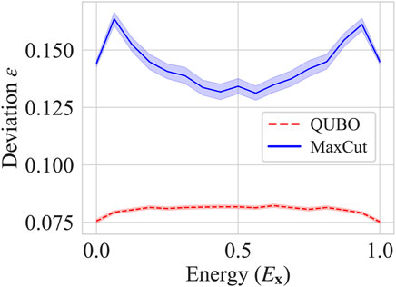
FIGURE 5. Deviation of the structure of the energy levels of the Ising models p(H, E; x) from the multivariate normal distribution along the energy spectrum. The deviation from normality at each point is defined as ${ϵ}_{\mathbf{x}}=\frac{1}{\#quantiles}{\sum }_{q-\text{quantiles}}|q-\text{quantile}\left(D_M^2\right)-q-\text{quantile}\left({\chi }_2^2\right)|$, where #quantiles is the number of quantiles (500 in these results, as in Figure 4). This metric is intended to provide the same information as the quantile–quantile plots in Figure 4 in a quantitative form. In particular, we divide the energy spectrum into 16 intervals and calculate the deviation at the extremes of each interval. We plot the average results for 1,000 random instances of QUBO and MaxCut, with a 95% confidence interval in the average estimation. The energy of every sample is rescaled between 0 (ground state energy) and 1 (maximum energy).

Hence, returning to the probability amplitude of a single-layer QAOA on non-degenerate Ising models, Eq. 26 together with the probability distribution in Eq. 31 leads to the following interference amplitude:

$|F\left(\mathbf{x}\right){|}^2\propto \exp \left[Y\right],\text{\hspace{0.17em}with}Y=-{\gamma }^2{\sigma }_E^2+\left(r^2-\frac{{\pi }^2}{4}\right){\sigma }_H^2-2r{\mu }_H-\gamma \pi \rho {\sigma }_E{\sigma }_H.(36)$

3.2.2 Degenerate Ising models

The MaxCut problems are a family of combinatorial optimization problems consisting of minimizing the following objective function:

$E_{\text{MaxCut}}\left(\mathbf{x}\right)=-2{\displaystyle \sum _{i,j}}{x}_i{Q}_{ij}\left(1-x_j\right),(37)$

with x ∈ {0,1}^N and Q is an N-by-N square matrix. Finding the minimum or an approximate solution very close to the minimum is known to be NP-hard (Håstad, 2001). Again, we can map the binary cost function optimization in Eq. 37 to an equivalent spin Hamiltonian optimization (Eq. 27):

${\tilde{E}}_{\text{MaxCut}}=-2{\displaystyle \sum _{i,j}}{x}_i{Q}_{ij}\left(1-x_j\right)+{\displaystyle \sum _{i,j}}\frac{1}{2}{Q}_{i,j}=\frac{1}{2}{\displaystyle \sum _{i,j=1}^N}{s}_i{J}_{ij}{s}_j,(38)$

where J = Q, and the magnetic field h cancels out. As in the non-degenerate case, the non-zero coefficients of Q are drawn from N(μ = 0, σ² = 1). This class of problems includes the Sherrington–Kirkpatrick model (Sherrington and Kirkpatrick, 1975) when all vertices of the graph are connected; that is, when the coupling matrix has no null coefficients.

In contrast to QUBO, the cost function in Eq. 38 exhibits a global ${\mathbb{Z}}_2$ symmetry that keeps invariant the energy under a global spin flip ${\tilde{E}}_{\text{MaxCut}}(\mathbf{s})={\tilde{E}}_{\text{MaxCut}}(-\mathbf{s})$, or what is the same, ${\tilde{E}}_{\text{MaxCut}}(\mathbf{x})={\tilde{E}}_{\text{MaxCut}}(1-\mathbf{x})$. In the non-degenerate scenario (Eq. 29), the presence of the magnetic field h breaks the symmetry. The existence of such global symmetries in the Hamiltonian results in the division of the Hilbert space into two or more distinct hierarchies of eigenstates. Note that if ${\mathbf{x}}^a=(x_1^a,x_2^a,\dots )$ represents a ground state, then there is another ground state in the opposite sector x^b = 1 − x^a. Consequently, a single excited state x′ can be seen now as arising from flipping spins in either of the ground states x^a or x^b. Accordingly, an identical spin configuration exhibits significantly different Hamming distances to both ground states, while its energy remains unchanged. Specifically, the Hamming distance reaches its maximum when considering the separation between the two degenerate ground states, where $H_{{\mathbf{x}}^a{\mathbf{x}}^b}=N$. Then, this symmetry implies that given any two states x and x′, there is a unique alternative state x″ such that E_x′ = E_x″ and $H_{\mathbf{x}{\mathbf{x}}^{\prime }}=N-H_{\mathbf{x}{\mathbf{x}}^{″}}$.

This phenomenon results in the separation of the probability distribution into a sum of two distributions, each measured with respect to one of the eigenstate hierarchies,

$p\left(H,E;\mathbf{x}\right)=p_{+}\left(H_{\mathbf{x},{\mathbf{x}}^{\prime }},E_{{\mathbf{x}}^{\prime }};\mathbf{x}\right)+p_{-}\left(H_{\mathbf{x},{\mathbf{x}}^{\prime }},E_{{\mathbf{x}}^{\prime }};\mathbf{x}\right),(39)$

where

$p_{+}\left(H,E;\mathbf{x}\right)=\frac{1}{2^{N/2}}{\displaystyle \sum _{{\mathbf{x}}^{\prime }\in \mathcal{A}}}\delta \left(H-H_{{\mathbf{xx}}^{\prime }}\right)\delta \left(E-E_{{\mathbf{x}}^{\prime }}\right),(40)$

$p_{-}\left(H,E;\mathbf{x}\right)=\frac{1}{2^{N/2}}{\displaystyle \sum _{{\mathbf{x}}^{\prime }\in \mathcal{B}}}\delta \left(H-H_{{\mathbf{xx}}^{\prime }}\right)\delta \left(E-E_{{\mathbf{x}}^{\prime }}\right),(41)$

with $\mathcal{A}$ and $\mathcal{B}$ being two complementary subspaces in the bit configurations space that represent the two eigenstate hierarchies. Because each distribution $p_{\pm }(H_{\mathbf{x},{\mathbf{x}}^{\prime }},E_{{\mathbf{x}}^{\prime }};\mathbf{x})$ defines itself a non-degenerate Hilbert subspace, it is natural to expect that they individually behave similarly to the probability distribution of the non-degenerate scenario explained in the previous section. Indeed, as shown in Figure 3, these distributions resemble two shifted bivariate Gaussian distributions:

$p_{+}{\left(H,E;\mathbf{x}\right)}_{{\rho }_{+}}\approx \frac{\exp \left[-\frac{1}{2\left(1-{\rho }_{+}^2\right)}\left({\left(\frac{E}{{\sigma }_E}\right)}^2+{\left(\frac{H-{\mu }_H+h_0}{{\sigma }_H}\right)}^2-2{\rho }_{+}\frac{E\left(H-{\mu }_H+h_0\right)}{{\sigma }_E{\sigma }_H}\right)\right]}{2\pi {\sigma }_E{\sigma }_H\sqrt{1-{\rho }_{+}^2}},(42)$

$p_{-}{\left(H,E;\mathbf{x}\right)}_{{\rho }_{-}}=p_{+}{\left(-H+2{\mu }_H,E;\mathbf{x}\right)}_{{\rho }_{+}},(43)$

$\approx \frac{\exp \left[-\frac{1}{2\left(1-{\rho }_{+}^2\right)}\left({\left(\frac{E}{{\sigma }_E}\right)}^2+{\left(\frac{H-{\mu }_H-h_0}{{\sigma }_H}\right)}^2+2{\rho }_{+}\frac{E\left(H-{\mu }_H-h_0\right)}{{\sigma }_E{\sigma }_H}\right)\right]}{2\pi {\sigma }_E{\sigma }_H\sqrt{1-{\rho }_{+}^2}},(44)$

where μ_E, μ_H, and σ_H are the same as Eq. 32, h₀ > 0 is a constant shift, and we have two separate correlation factors ρ₊(x) = −ρ₋(x) ≡ ρ. As in QUBO, we prove the Gaussian distribution of the eigenstates by a multivariate normality test based on the Mahalanobis distance. In this case, we first need to group the states into two clusters that represent $\mathcal{A}$ and $\mathcal{B}$ hierarchies. As previously explained, we do this by fitting the sample points $\mathbf{s}=(H_{\mathbf{x}{\mathbf{x}}^{\prime }},E_{{\mathbf{x}}^{\prime }})$ to a mixture of two Gaussians so that we identify which states should belong to p₊ or p₋. Then, we calculate the Mahalanobis distance of all samples using their corresponding mean and covariance estimated from the Gaussian mixture fit. Again, we find a good correspondence between the Mahalanobis distance and the ${\chi }_2^2$ distribution for the vast majority of the energy spectrum and conclude that p_±(H, E; x) are well approximated by the Gaussian expressions in Eqs 42, 44.

As in the non-degenerate case, the correlation factors ρ_± encapsulate the entire dependency in x, but we now have two functions that influence one another. Equation 22 along this p₊, p₋ interference leads to

$|F\left(\mathbf{x}\right){|}^2\propto \exp \left[Y^{\prime }\right]\cdot \left(\cos \left(h_0\pi +2r\gamma \rho {\sigma }_E{\sigma }_H\right)+\cosh \left(2h_{0}r-\gamma \pi \rho {\sigma }_E{\sigma }_H\right)\right),\text{\hspace{0.17em}with}(45)$

$Y^{\prime }\equiv -{\gamma }^2{\sigma }_E^2+\left(r^2-\frac{{\pi }^2}{4}\right){\sigma }_H^2-2r{\mu }_H.(46)$

Therefore, we observe that the interference translates into a mixture of two exponentials together with an oscillatory term

$2\cosh \left(2h_{0}r-\gamma \pi \rho {\sigma }_E{\sigma }_H\right)=\exp \left[{\beta }^{\prime }\rho +2h_{0}r\right]+\exp \left[-{\beta }^{\prime }\rho -2h_{0}r\right],(47)$

with β′ ≡ − γπσ_Eσ_H. Nevertheless, except in the regime when r = − log(tan θ) ≈ 0 (θ ≈ π/4), one exponential is clearly dominant over the other due to the presence of the h₀-shift:

$\exp \left[{\beta }^{\prime }\rho +2h_{0}r\right]+\exp \left[-{\beta }^{\prime }\rho -2h_{0}r\right]\approx \exp \left[\mathrm{s}\mathrm{g}\mathrm{n}\left(r\right){\beta }^{\prime }\left({\rho }_{+}+{\rho }_{-}\right)+\mathrm{s}\mathrm{g}\mathrm{n}\left(r\right)2h_{0}r\right],(48)$

where sgn(⋅) is the sign function. Thus, the interference amplitude in Eq. 45 becomes

$|F\left(\mathbf{x}\right){|}^2\propto \exp \left[Y^{\prime }\right]\cdot \exp \left[\mathrm{s}\mathrm{g}\mathrm{n}\left(r\right){\beta }^{\prime }\rho \right]=\exp \left[Y\right],\text{\hspace{0.17em}with}(49)$

$Y=-{\gamma }^2{\sigma }_E^2+\left(r^2-\frac{{\pi }^2}{4}\right){\sigma }_H^2-2r{\mu }_H-\mathrm{s}\mathrm{g}\mathrm{n}\left(r\right)\gamma \pi {\sigma }_E{\sigma }_H\rho .(50)$

Note that this formula is consistent with the non-degenerate scenario in Eq. 36 except for small corrections caused by the merging of eigenstate hierarchies (see Eq. 48) and the role of r that defines two different regimes for $\theta \in \left(0,\frac{\pi }{4}\right)$ and $\theta \in \left(\frac{\pi }{4},\frac{\pi }{2}\right)$.

4 QAOA thermal-like distributions

The interferometric model, in combination with the approximate Gaussian correlations between energy and Hamming distance, is a powerful tool that allows us to approximate the probability distribution generated by the QAOA variational circuit. In the following discussion, we will indeed show that, with minimal assumptions, the single-layer QAOA state approximates a Boltzmann distribution with effective temperature determined by the γ and θ angles, as shown by Díez-Valle et al. (2023).

To achieve this goal, we analyze the single-layer QAOA interference amplitudes (Eqs 36, 49) in energy space

$P\left(E\right)={\displaystyle \sum _{\mathbf{x}}}\delta \left(E-E_{\mathbf{x}}\right)|F\left(\mathbf{x}\right){|}^2.(51)$

In order to examine this probability amplitude distribution of energy states, we should only pay attention to the terms of |F(x)|² that are influenced by the spin configuration x and its associated energy E_x. In the previous section, we derived that the single-layer QAOA probability amplitude of Ising Hamiltonian eigenstates for both non-degenerate and degenerate spectra can be expressed as

$|F\left(\mathbf{x}\right){|}^2\propto \exp \left[-{\gamma }^2{\sigma }_E^2+\left(r^2-\frac{{\pi }^2}{4}\right){\sigma }_H^2-2r{\mu }_H-\gamma \pi \rho {\sigma }_E{\sigma }_H\right],(52)$

where ρ = σ_EH/(σ_Eσ_H) with σ_EH = sgn(r)σ_EH in the degenerate scenario. As previously mentioned, the correlation factor captures the whole variability of Eq. 52 in energy space. All the other terms are set by the spin model and are, therefore, independent of the state x. The only contributing part to the amplitude is

$-\gamma \pi \rho {\sigma }_E{\sigma }_H=-\gamma \pi {\sigma }_{EH}\left(\mathbf{x}\right).(53)$

Hence, in terms of the distribution in energy space, we can write the quantum probability amplitude as the following exponential:

$|F\left(\mathbf{x}\right){|}^2\propto e^{-\gamma \pi {\sigma }_{EH}\left(\mathbf{x}\right)}.(54)$

Let us recall that σ_EH(x) represents the covariance between the Hamming distance from excited x′ to the reference state x and its energy $E_{{\mathbf{x}}^{\prime }}$ (Eq. 30). The place of x in the energy spectrum is highly correlated with σ_EH(x). In non-degenerate spaces, when x is the ground/highest energy state, it is more likely to find low/high energy states $\left((E_{{\mathbf{x}}^{\prime }}-\mathbb{E}[E])<0/(E_{{\mathbf{x}}^{\prime }}-\mathbb{E}[E])>0\right)$ close to the reference state $\left((H_{\mathbf{x}{\mathbf{x}}^{\prime }}-\mathbb{E}[H])<0\right)$ and high/low energy states far from the reference state $\left((H_{\mathbf{x}{\mathbf{x}}^{\prime }}-\mathbb{E}[H])>0\right)$, leading to a high positive/negative covariance. In the degenerate scenario, we have the same behavior for subspace p₊ and the exact opposite for the complementary subspace $p_{-}\left(H_{\mathbf{x}{\mathbf{x}}^{\prime }}\to -H_{\mathbf{x}{\mathbf{x}}^{\prime }}+2{\mu }_H\right)$. This intuition translates into an evident σ_EH − E_x correlation that can be numerically observed in Figure 4 of Díez-Valle et al. (2023). This dependence can be expressed as the sum of a linear function and a stochastic value ω with zero mean:

${\sigma }_{EH}\left(\mathbf{x}\right)=-c\cdot E_{\mathbf{x}}\pm \omega ,(55)$

where $c\in \mathbb{R}>0$. Despite the presence of the random term ω, the trend in Eq. 55 is noticeable. Therefore, introducing Eq. 55 into Eq. 54 leads to a thermal-like probability amplitude distribution for the Ising models:

$|F\left(\mathbf{x}\right){|}^2\propto e^{-\beta E_{\mathbf{x}}\pm \beta \omega /c},(56)$

where β = cπγ for non-degenerate problems and β = sgn(r)cπγ for degenerate ones play the role of the inverse temperature. Then, the probability distribution in energy space can be expressed as

$P\left(E\right)\sim d\left(E\right)e^{-\beta E},(57)$

where d(E) is the density of states that in Ising models resembles a normal distribution centered in intermediate energies.

The Boltzmann distribution in Eq. 56, together with the random fluctuations ω, manifests in regimes of optimized parameters, but the distribution may be modified by manipulating the angles θ ∈ (0, π/2) and γ (see Figures 6, 7). By analyzing Eq. 56 and previous expressions, additional conclusions can be drawn about the shape of the distribution.

• The angle γ controls the direction of the optimization. For specific γ regimes, the single-layer QAOA probability amplitude distribution on Ising models resembles a thermal distribution at temperature $T={\beta }^{-1}=\frac{1}{c\pi |\gamma |}$ such that the ground state of the system aligns with the peak amplitude. Switching the sign of this angle is the same as changing the sign of the energy and, therefore, of the temperature $T=\frac{-1}{c\pi |\gamma |}$. These negative temperature states increase the probability of the highest excited state.

• The degenerate Ising models exhibit antisymmetric behavior at the angle θ because $T=\frac{\mathrm{s}\mathrm{g}\mathrm{n}}{c\pi |\gamma |}$, with r = − log(tan θ). Therefore, for θ < π/4 and θ > π/4, the pure QAOA state resembles a thermal-like distribution with positive/negative temperature. Equation 45 shows that when θ ≈ π/4, the thermal type distribution disappears, and we find a mixture of two Boltzmann exponentials with opposite temperatures. This behavior can be observed in Figure 7B.

• The Boltzmann distribution is apparent for a finite interval of angles γ ∈ (0, γ_c]. The lowest temperature T is reached near γ ≈ γ_opt, where γ_opt is the angle that minimizes the mean energy in the variational principle. The random noise βω/c = πγω in Eq. 56 grows with γ so that the smaller the γ, the lower the noise and the more noticeable the Boltzmann distribution. When |γ| > γ_c, the fluctuations are such that the Boltzmann term becomes marginal.

• For γ < γ_c, we observe that β grows linearly with the angle γ, consistent with the numerical results of Díez-Valle et al. (2023).

FIGURE 6

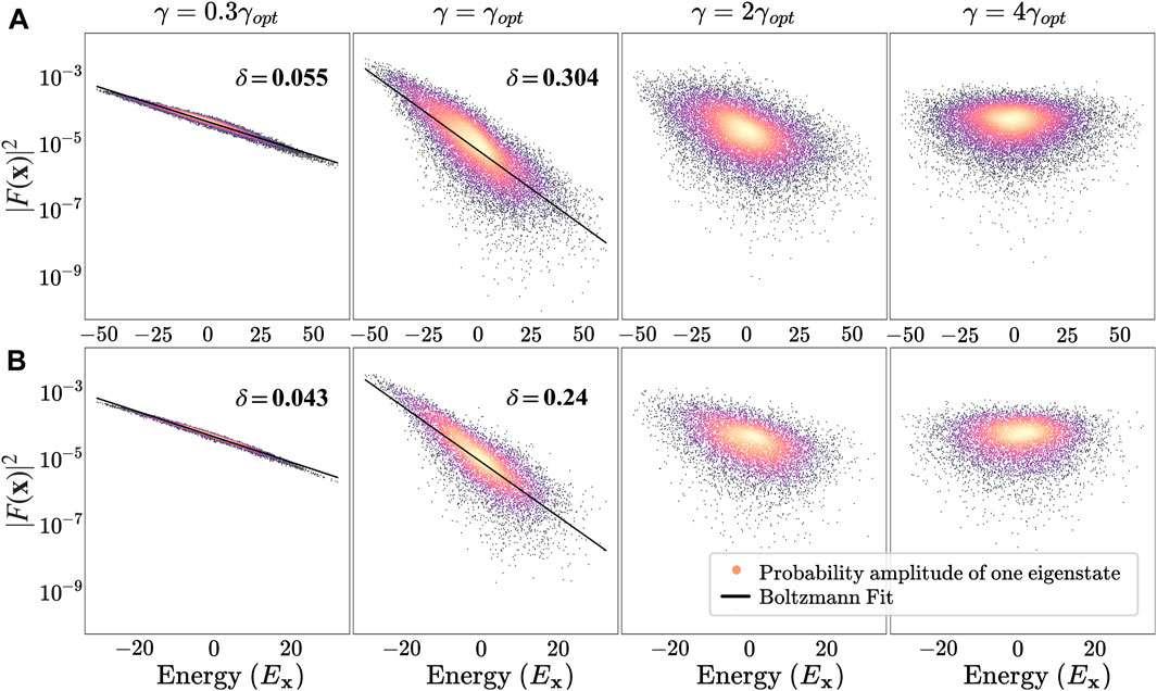
FIGURE 6. Evolution of the single-layer QAOA probability amplitude distribution as we modify the angle γ with optimal θ. We plot the probabilities |F(x)|² versus their energies E_x for a single random instance of a 14-qubit (A) QUBO (γ_opt = −0.09 and θ_opt ≈ π/6) and (B) a MaxCut (γ_opt = −0.14 and θ_opt ≈ π/8) Hamiltonian. The optimal angles (γ_opt, θ_opt) are those that minimize the mean energy ⟨E⟩ = ∑_x|F(x)|²E_x. Note how a Boltzmann distribution with perturbations is apparent for γ ≤ γ_opt. We also display the total variation distance δ between the single-layer QAOA probability distribution and the Boltzmann distribution fit $\delta =\frac{1}{2}{\sum }_{\mathbf{x}}\Vert F(\mathbf{x}){|}^2-e^{-{\beta }_{\text{fit}}{E}_{\mathbf{x}}}/\mathcal{Z}|$, with $\mathcal{Z}={\sum }_{\mathbf{x}}{e}^{{\beta }_{\text{fit}}{E}_{\mathbf{x}}}$ being the partition function.

FIGURE 7

FIGURE 7. Single-layer QAOA probability amplitude distribution with optimal γ in different regimes of the angle θ. We plot the probabilities |F(x)|² versus their energies E_x for a single random instance of a 14-qubit (A) QUBO (γ_opt = −0.09 and θ_opt ≈ π/6) and (B) MaxCut (γ_opt = −0.14 and θ_opt ≈ π/8) Hamiltonian. The optimal angles (γ_opt, θ_opt) are those that minimize the mean energy ⟨E⟩ = ∑_x|F(x)|²E_x. We also display the total variation distance δ between the single-layer QAOA probability distribution and the Boltzmann distribution fit $\delta =\frac{1}{2}{\sum }_{\mathbf{x}}\Vert F(\mathbf{x}){|}^2-e^{-{\beta }_{\text{fit}}{E}_{\mathbf{x}}}/\mathcal{Z}|$, with $\mathcal{Z}={\sum }_{\mathbf{x}}{e}^{{\beta }_{\text{fit}}{E}_{\mathbf{x}}}$ being the partition function.

5 Outlook

Sampling from complex probability distributions is a valuable computational task, both for its difficulty and its broad applicability. Quantum states projected on the computational basis are, in essence, classical probability distributions, and measuring them is the same as sampling from such distributions. Therefore, a quantum computer can be roughly seen as a machine capable of creating exotic or suitable probability distributions thanks to quantum phenomena. Indeed, the first claim of quantum supremacy (Preskill, 2018) was performed on a sampling problem (Arute et al., 2019), and this task has also been envisioned as one of the candidates to show a practical quantum advantage in the near term (Wu et al., 2021; Zhong et al., 2021; Layden et al., 2023).

In this context, the Boltzmann distributions of Ising models could be good candidates to show such quantum advantage for two reasons. First, these distributions are classically intractable at low-temperature regimes. The most popular strategy to simulate thermal distributions is the use of Markov chain Monte Carlo (MCMC) algorithms that guarantee convergence to the Boltzmann distribution at a given temperature T. While these methods work very well for relatively high temperatures, the number of iterations needed to converge scales exponentially when the temperature is too low. Much effort has been expended to determine the range of temperatures that ensure rapid mixing and, therefore, the polynomial convergence of MCMCs. To the best of our knowledge, the state-of-the-art theoretical bound indicates that an MCMC always converges in polynomial time to the thermal distribution of an Ising model at a temperature higher than ‖J‖ (Eldan et al., 2021), although practical realizations and state-of-the-art methods (e.g., parallel tempering and population annealing) might overcome this threshold. Díez-Valle et al. (2023) showed that the single-layer QAOA already approximates Boltzmann distributions at temperatures beyond this theoretical MCMC bound.

Second, a wide range of fields would be impacted by an improvement in Boltzmann distribution sampling. In statistical mechanics, sampling from this distribution is crucial for simulating physical systems at thermal equilibrium and for computing observables such as magnetization in Ising models. Furthermore, machine learning uses this distribution in unsupervised learning techniques known as Boltzmann machines (Ackley et al., 1985). Combinatorial optimization is another field of interest because some algorithms employ Boltzmann distribution sampling at decreasing temperatures as a subroutine to find the minimum of a cost function (Kirkpatrick et al., 1983).

The thermal-like distributions of the single-layer QAOA reveal a nice connection between quantum algorithmics and statistical physics that can help gain a better understanding of the behavior of these ansatzes. However, from a broader perspective, the QAOA sampling from approximate Boltzmann distributions, also known as Gibbs sampling, may be extended to the multilayer scenario with an improvement in the achievable temperature (Lotshaw et al., 2022) or to QAOA mixed-state ansatzes to train unsupervised learning models as implemented in Verdon et al. (2019). Furthermore, because the QAOA resembles a Trotterized approximation to an adiabatic quantum evolution, this picture might be expanded to the infinite depth scenario p → ∞ and the engineering of general time-dependent adiabatic passages.

Additionally, the approximate Boltzmann distributions of single-layer QAOA states present collateral implications in quantum information theory. For example, this behavior makes them suitable as warm initial states for more complex ansatzes, as demonstrated in Leontica and Amaro (2023). Another recent work (Sud et al., 2022) shows how a tight dependence between the energy distribution of the spin model and the final probability amplitude of the QAOA states allows a more efficient classical heuristic optimization of the QAOA parameters. The Boltzmann distribution unambiguously connects the energy of the eigenstates with their amplitudes, thus providing further arguments and explanations on these heuristics.

We are confident that this study and earlier work by Díez-Valle et al. (2023) are two initial works in a new field in which variational and other types of circuits are analyzed from a physical perspective, understanding not only their computational power but also offering potentially significant physical insights into the quantum computer’s dynamics.

Data availability statement

The original contributions presented in the study are included in the article/Supplementary Material; further inquiries can be directed to the corresponding author.

Author contributions

PD-V: Conceptualization, Formal analysis, Investigation, writing–original draft. DP: Conceptualization, Funding acquisition, Supervision, writing–review and editing. JG-R: Conceptualization, Funding acquisition, Project administration, Software, Supervision, writing–review and editing.

Funding

The authors declare that financial support was received for the research, authorship, and/or publication of this article. This work was supported by the European Commission FET Open project AVaQus Grant Agreement 899561, the Proyecto Sinérgico CAM 2020 Y2020/TCS-6545 (NanoQuCoCM), the Spanish CDTI through Misiones Ciencia e Innovación Program (CUCO) under Grant MIG-20211005, and the CSIC Interdisciplinary Thematic Platform (PTI) Quantum Technologies (PTI-QTEP).

Conflict of interest

The authors declare that the research was conducted in the absence of any commercial or financial relationships that could be construed as a potential conflict of interest.

Publisher’s note

All claims expressed in this article are solely those of the authors and do not necessarily represent those of their affiliated organizations, or those of the publisher, the editors, and the reviewers. Any product that may be evaluated in this article, or claim that may be made by its manufacturer, is not guaranteed or endorsed by the publisher.

References

Ackley, D. H., Hinton, G. E., and Sejnowski, T. J. (1985). A learning algorithm for Boltzmann machines. Cognitive Sci. 9, 147–169. doi:10.1016/S0364-0213(85)80012-4

CrossRef Full Text | Google Scholar

Albash, T., and Lidar, D. A. (2018). Adiabatic quantum computation. Rev. Mod. Phys. 90, 015002. doi:10.1103/revmodphys.90.015002

CrossRef Full Text | Google Scholar

Arute, F., Arya, K., Babbush, R., Bacon, D., Bardin, J. C., Barends, R., et al. (2019). Quantum supremacy using a programmable superconducting processor. Nature 574, 505–510. doi:10.1038/s41586-019-1666-5

PubMed Abstract | CrossRef Full Text | Google Scholar

Barahona, F. (1982). On the computational complexity of ising spin glass models. J. Phys. A Math. General 15, 3241–3253. doi:10.1088/0305-4470/15/10/028

CrossRef Full Text | Google Scholar

Bharti, K., Cervera-Lierta, A., Kyaw, T. H., Haug, T., Alperin-Lea, S., Anand, A., et al. (2022). Noisy intermediate-scale quantum algorithms. Rev. Mod. Phys. 94, 015004. doi:10.1103/revmodphys.94.015004

CrossRef Full Text | Google Scholar

Blekos, K., Brand, D., Ceschini, A., Chou, C.-H., Li, R.-H., Pandya, K., et al. (2023). A review on quantum approximate optimization algorithm and its variants. arXiv:2306.09198

Google Scholar

Bremner, M. J., Jozsa, R., and Shepherd, D. J. (2010). Classical simulation of commuting quantum computations implies collapse of the polynomial hierarchy. Proc. R. Soc. A Math. Phys. Eng. Sci. 467, 459–472. doi:10.1098/rspa.2010.0301

CrossRef Full Text | Google Scholar

Bremner, M. J., Montanaro, A., and Shepherd, D. J. (2016). Average-case complexity versus approximate simulation of commuting quantum computations. Phys. Rev. Lett. 117, 080501. doi:10.1103/physrevlett.117.080501

PubMed Abstract | CrossRef Full Text | Google Scholar

Brod, D. J. (2015). Complexity of simulating constant-depth BosonSampling. Phys. Rev. A 91, 042316. doi:10.1103/physreva.91.042316

CrossRef Full Text | Google Scholar

Cerezo, M., Arrasmith, A., Babbush, R., Benjamin, S. C., Endo, S., Fujii, K., et al. (2021). Variational quantum algorithms. Nat. Rev. Phys. 3, 625–644. doi:10.1038/s42254-021-00348-9

CrossRef Full Text | Google Scholar

Díez-Valle, P., Porras, D., and García-Ripoll, J. J. (2023). Quantum approximate optimization algorithm pseudo-Boltzmann states. Phys. Rev. Lett. 130, 050601. doi:10.1103/physrevlett.130.050601

PubMed Abstract | CrossRef Full Text | Google Scholar

Eldan, R., Koehler, F., and Zeitouni, O. (2021). A spectral condition for spectral gap: fast mixing in high-temperature ising models. Probab. Theory Relat. Fields 182, 1035–1051. doi:10.1007/s00440-021-01085-x

CrossRef Full Text | Google Scholar

Farhi, E., Goldstone, J., and Gutmann, S. (2014). A quantum approximate optimization algorithm. 1411.4028. doi:10.48550/arxiv.1411.4028

CrossRef Full Text | Google Scholar

Farhi, E., Goldstone, J., Gutmann, S., Lapan, J., Lundgren, A., and Preda, D. (2001). A quantum adiabatic evolution algorithm applied to random instances of an np-complete problem. Science 292, 472–475. doi:10.1126/science.1057726

PubMed Abstract | CrossRef Full Text | Google Scholar

Farhi, E., Goldstone, J., Gutmann, S., and Sipser, M. (2000). Quantum computation by adiabatic evolution. arXiv.quant-ph/0001106

Google Scholar

Farhi, E., Goldstone, J., Gutmann, S., and Zhou, L. (2022). The quantum approximate optimization algorithm and the sherrington-kirkpatrick model at infinite size. Quantum 6, 759. doi:10.22331/q-2022-07-07-759

CrossRef Full Text | Google Scholar

Farhi, E., and Harrow, A. W. (2019). Quantum supremacy through the quantum approximate optimization algorithm. arXiv:1602.07674.

Google Scholar

Harrigan, M. P., Sung, K. J., Neeley, M., Satzinger, K. J., Arute, F., Arya, K., et al. (2021). Quantum approximate optimization of non-planar graph problems on a planar superconducting processor. Nat. Phys. 17, 332–336. doi:10.1038/s41567-020-01105-y

CrossRef Full Text | Google Scholar

Håstad, J. (2001). Some optimal inapproximability results. J. ACM 48, 798–859. doi:10.1145/502090.502098

CrossRef Full Text | Google Scholar

Kirkpatrick, S., Gelatt, C., and Vecchi, M. (1983). Optimization by simulated annealing. Sci. (New York, N.Y.) 220, 671–680. doi:10.1126/science.220.4598.671

PubMed Abstract | CrossRef Full Text | Google Scholar

Kochenberger, G., Glover, F., Rego, C., et al. (2004). A unified modeling and solution framework for combinatorial optimization problems. OR Spectr. 26, 237–250. doi:10.1007/s00291-003-0153-3

CrossRef Full Text | Google Scholar

Kochenberger, G., Hao, J., Lewis, M., Lü, Z., Wang, H., et al. (2014). The unconstrained binary quadratic programming problem: a survey. J. Comb. Optim. 28, 58–81. doi:10.1007/s10878-014-9734-0

CrossRef Full Text | Google Scholar

Layden, D., Mazzola, G., Mishmash, R. V., Motta, M., Wocjan, P., Kim, J.-S., et al. (2023). Quantum-enhanced Markov chain Monte Carlo. Nature 619, 282–287. doi:10.1038/s41586-023-06095-4

PubMed Abstract | CrossRef Full Text | Google Scholar

Leontica, S., and Amaro, D. (2023). Exploring the neighborhood of 1-layer QAOA with instantaneous quantum polynomial circuits. Phys. Rev. Research arXiv:2210.05526

Google Scholar

Lotshaw, P. C., Siopsis, G., Ostrowski, J., Herrman, R., Alam, R., Powers, S., et al. (2022). Approximate Boltzmann distributions in quantum approximate optimization. Phys. Rev. arXiv:2212.01857

Google Scholar

Lucas, A. (2014). Ising formulations of many NP problems. Front. Phys. 2. doi:10.3389/fphy.2014.00005

CrossRef Full Text | Google Scholar

Lund, A. P., Bremner, M. J., and Ralph, T. C. (2017). Quantum sampling problems, BosonSampling and quantum supremacy. npj Quantum Inf. 3, 15. doi:10.1038/s41534-017-0018-2

CrossRef Full Text | Google Scholar

Mahalanobis, P. C. (1936). On the generalised distance in statistics. Proc. Natl. Inst. Sci. India 2, 49. doi:10.1007/s13171-019-00164-5

CrossRef Full Text | Google Scholar

Moll, N., Barkoutsos, P., Bishop, L. S., Chow, J. M., Cross, A., Egger, D. J., et al. (2018). Quantum optimization using variational algorithms on near-term quantum devices. Quantum Sci. Technol. 3, 030503. doi:10.1088/2058-9565/aab822

CrossRef Full Text | Google Scholar

Nannicini, G. (2019). Performance of hybrid quantum-classical variational heuristics for combinatorial optimization. Phys. Rev. E 99, 013304. doi:10.1103/physreve.99.013304

PubMed Abstract | CrossRef Full Text | Google Scholar

Nemhauser, G. L., and Wolsey, L. A. (1988). Integer and combinatorial optimization. USA: John Wiley & Sons, Ltd.

Google Scholar

Ozaeta, A., van Dam, W., and McMahon, P. L. (2022). Expectation values from the single-layer quantum approximate optimization algorithm on ising problems. Quantum Sci. Technol. 7, 045036. doi:10.1088/2058-9565/ac9013

CrossRef Full Text | Google Scholar

Pedregosa, F., Varoquaux, G., Gramfort, A., Michel, V., Thirion, B., Grisel, O., et al. (2011). Scikit-learn: machine learning in Python. J. Mach. Learn. Res. 12, 2825–2830.

Google Scholar

Preskill, J. (2018). Quantum computing in the NISQ era and beyond. Quantum 2, 79. doi:10.22331/q-2018-08-06-79

CrossRef Full Text | Google Scholar

Sherrington, D., and Kirkpatrick, S. (1975). Solvable model of a spin-glass. Phys. Rev. Lett. 35, 1792–1796. doi:10.1103/PhysRevLett.35.1792

CrossRef Full Text | Google Scholar

Sud, J., Hadfield, S., Rieffel, E., Tubman, N., and Hogg, T. (2022). A parameter setting heuristic for the quantum alternating operator ansatz. Phys. Rev. Research. arXiv:2211.09270.

Google Scholar

Sung, K. J., Yao, J., Harrigan, M. P., Rubin, N. C., Jiang, Z., Lin, L., et al. (2020). Using models to improve optimizers for variational quantum algorithms. Quantum Sci. Technol. 5, 044008. doi:10.1088/2058-9565/abb6d9

CrossRef Full Text | Google Scholar

Verdon, G., Broughton, M., and Biamonte, J. (2019). A quantum algorithm to train neural networks using low-depth circuits. 1712. 05304, doi:10.48550/arXiv.1712.05304

CrossRef Full Text | Google Scholar

Wild, D. S., Sels, D., Pichler, H., Zanoci, C., and Lukin, M. D. (2021). Quantum sampling algorithms for near-term devices. Phys. Rev. Lett. 127, 100504. doi:10.1103/physrevlett.127.100504

PubMed Abstract | CrossRef Full Text | Google Scholar

Wu, Y., Bao, W.-S., Cao, S., Chen, F., Chen, M.-C., Chen, X., et al. (2021). Strong quantum computational advantage using a superconducting quantum processor. Phys. Rev. Lett. 127, 180501. doi:10.1103/physrevlett.127.180501

PubMed Abstract | CrossRef Full Text | Google Scholar

Zhong, H.-S., Deng, Y.-H., Qin, J., Wang, H., Chen, M.-C., Peng, L.-C., et al. (2021). Phase-programmable Gaussian boson sampling using stimulated squeezed light. Phys. Rev. Lett. 127, 180502. doi:10.1103/physrevlett.127.180502

PubMed Abstract | CrossRef Full Text | Google Scholar