Non-linearity in Marginal LCA: Application of a Spatial Optimization Model

Introduction

Despite its immense successes, modern agriculture is also driving our planet beyond its safe operating space (Campbell et al., 2017). It contributes considerably to an array of global problems, from climate change, air pollution, water quality deterioration, to biodiversity loss (Tilman et al., 1994; Ongley, 1996; Mosier et al., 1998; Aneja et al., 2009; Qin and Horvath, 2020a; Suh et al., 2020; Tao et al., 2020). The search is on for sustainable strategies across the food supply chain to reduce agriculture's environmental impacts (Tilman et al., 2001; Mueller et al., 2012; Springmann et al., 2018; Dai et al., 2020; Qin and Horvath, 2020b). One strategy that has received increasing attention is a dietary shift toward healthy foods (Pimentel and Pimentel, 2003; Tilman and Clark, 2014; Springmann et al., 2016; Godfray et al., 2018; Willett et al., 2019). However, how to accurately determine the potential environmental benefits of such a dietary shift remain debated and unclear (Plevin et al., 2014; Cucurachi et al., 2016; Yang and Campbell, 2017).

Life-cycle assessment (LCA) is the main approach used to measure foods' environmental performance and then based on their differences to infer environmental benefits, costs, or tradeoffs between different food choices and diets (Weber and Matthews, 2008; Roy et al., 2009; Tilman and Clark, 2014). But this approach may fall short for this purpose (Cucurachi et al., 2016). Food LCAs reflect the total resource use and emissions of existing food systems across the supply chain. By suggesting (i) we should consume more A and less B because food A is “greener” than food B and (ii) this would result in certain benefits as reflected in their different LCA results, this approach implicitly assumes that one more unit of A will have the same life-cycle impacts as an existing, average unit of A (the same for one less unit of B). In other words, this approach linearly extrapolates from existing food data to estimate marginal life-cycle impacts resulting from a change in food consumption (Suh and Yang, 2014; Yang, 2016; Brandao et al., 2017). And the linearity rests on further assumptions, including fixed input-output relations for all life-cycle processes involved and an unlimited supply of inputs (West, 1995; Yang, 2016; Boulay et al., 2020; Forin et al., 2020; Heijungs, 2020). This linear approach would suffice when the assumptions largely hold true but could be problematic when they are severely violated. In the case of food, because agricultural production has a high system variability and is constrained by land, marginal emissions can be considerably different from the average (Yang, 2016). In our study, marginal LCA refers to the impacts of changes in the output of products from the system, while average LCA represents the average impacts for producing a unit of products in a system. The non-linear relationship between demand and impacts is usually overlooked in LCA studies. Therefore, we need to understand the non-linear marginal changes in order to better determine the consequences of dietary changes.

Owing to the complexity of the human-environment system, marginal changes resulting from our decisions can be potentially influenced by many factors, from economic, social, to political, thus requiring an integrated approach to capture the possibilities. Economic aspects like production cost and consumer spending have traditionally been the focus of impact modeling (Dixon and Jorgenson, 2012), but social issues and considerations can also matter. For example, the rise of organic foods, despite higher prices, has been driven by concerns about health, environment, food safety, and taste (Massey et al., 2018). Moreover, policy per se plays an important role, and different policy interventions, even with the same goal, can lead to different outcomes. Rajagopal et al. (2011) showed that the production mandate and subsidy affects the biofuel-petroleum displacement ratio differently, highlighting that the environmental outcome of technology depends also on the policy regime.

Traditional consequential LCA studies rely on economic models such as partial equilibrium and computational general equilibrium, while they are mathematically complicated and only represent an aggregate resolution of the economy (Yang and Heijungs, 2018). The optimization method has been used recently to estimate the effects in a detailed process-level market (Gong and You, 2017; Garcia and You, 2018; Palazzo et al., 2020). For example, optimization models are applied in rice production and energy storage systems (Kätelhön et al., 2016; Elzein et al., 2019). However, the effects of change in demand involving producers and consumers from multiple regions have not been fully addressed in LCA studies. An integrated approach to marginal estimation should, therefore, take these into consideration, tailored to the particular question under study.

The main purpose of the study is to demonstrate this integrated approach. We applied the proposed approach to a preliminary case study of irrigation water use in marginal U.S. potato production, and the policy implications may be limited due to assumptions. In general, irrigation water dominates the blue water footprint of crops. Specifically, we estimate additional irrigation water use caused by a hypothetical increase in potato production, which could occur as a result of a shift toward plant-based diets. We build several scenarios at the state level to capture the possibilities of what could happen under different influences, from economic, social, to political perspectives. Below, we provide details on the scenarios, present key results, and conclude with implications of our study for LCA methodology development.

Materials and Methods

Overview

We model changes in potato demand due to a healthier diet as recommended by the U.S. Department of Agriculture (USDA) and how this would increase irrigation water use for potato production. To this end, we build four sets of production scenarios. The first is the average production pattern in which production in each state expands in proportion to its current level, reflecting the linear extrapolation method. The second is the marginal production pattern, reflecting additional potato would be produced by the most cost-competitive states which supply potatoes at low prices. The third is a high fuel price scenario, reflecting a growing trend of local and regional food systems in the U.S. (Low et al., 2015). The fourth is a high water price scenario, reflecting policy support of agricultural water conservation. Scenarios two to four are non-linear models and analyzed by minimizing cost under different constraints.

Data Sources and Assumptions

We build a model based on state-specific production technologies, constraints of production capacity, and additional demands. For this case study, we collected state-by-state data on potato demand, production, and transportation, including available land for potato cultivation, potato yield per acre of land, irrigation water use, and interstate transportation fuel costs. The key data and their sources are summarized in Table 1. Detailed data on cost and production can be found in the Supplementary Material. We used the state averages for those states which did not have data for production cost and irrigation water use.

TABLE 1

Table 1. Data sources and key assumptions of fresh potatoes.

Our cost estimates consist of two parts: production cost and transportation fuel cost. The production cost is from a USDA potato report (U.S. Department of Agriculture, 2016a), and interstate transportation fuel cost is the fuel cost consumed by transporting potato from the geographic center of a producing state to the geographic center of a consuming state (U.S. Energy Information Administration, 2019). The data of the centers of the states and interstate transportation distances were obtained from Google Map. The production cost includes the costs of materials, fertilizers, biocides, irrigation water, agricultural machinery, direct fuels, and labors. The high fuel price, $1.5 per liter, used in the high fuel price scenario, is estimated by EIA in the high oil price case for the year 2050 (U.S. Energy Information Administration, 2019). The high water price, $2.0 per m³, used in the high water price scenario, is estimated in a survey of annual water prices for selected cities in the U.S. (Bunch et al., 2017). We used the increase in water price from the high water scenario to the average water scenario, $1.1 per m³, in our study to demonstrate the effect of high water price.

Since potato can be grown almost in any types of soils and conditions, soil types and climates are not considered as constraints in this study. We find that production in a given year did not exceed 170% of the previous year in most states, so we cap the additional potato production in each state at 70% of its current production. Potato demand is determined by the USDA recommended amount and the current consumption quantity for each state.

Marginal Production and Scenario Analysis

In the study, we estimate the marginal production pattern for the additional demand of potatoes under the goal of minimizing cost that the total cost of producing and transporting potato across the nation is minimized. Three scenarios are developed to find where the additional potato production would occur, given that all states in the USA would likely seek to meet the additional demand at a minimum cost. Specifically, (1) in the marginal production scenario, potatoes may be produced from the state with the lowest total costs first and then from the state with second lowest cost; (2) in the high fuel price scenario, demand may be fulfilled by production within the state first and then from neighboring states; and (3) in the high water price scenario, water use may largely influence the location of production.

Optimization Models

The optimization problems of multi-agent systems belong to the class of problems referred to as transportation problems (Vignaux and Michalewicz, 1991; Ferguson, 2000). The transportation problem is a classic area in optimization. The transportation model is used to solve the problem of allocating commodity from sources where the supply of some commodity is available to destinations where the commodity is demanded. The transportation problem was first formalized by a French mathematician called Gaspard Monge in 1781 (Monge, 1781).

The main applications of transportation problems involve (1) minimizing transportation costs, (2) determining low-cost location, (3) finding minimum cost production schedule, and (4) optimizing distribution system. Nowadays, its applications have been expanded to many fields such as operations research, transportation and logistics research, chemical engineering, mathematics, and economics. The transportation model has a wide application in the field of operation research and management science to provide better planning and management from the location and allocation analysis (Conway and Maxwell, 1961; Cooper, 1963; Feldman et al., 1966; Scott, 1970).

The purpose of applying the transportation model in this study is to minimize the total cost of transportation and production so that the demand of each state is met and every producing state operates within its capacity. Suppose there are Istates, M₁ ... M_I, that produce potato, and there are Jstates, N₁ ... N_J, receiving potato to fulfill the additional demand determined by the dietary shift. Let x_ij be the quantity of potato shipped from state M_i to state N_j.

First, the quantity of potatoes supplied by producing state M_i to receiving state N_j is ${\displaystyle \sum _{j=1}^J}{x}_{ij}$, which cannot exceed the maximal amount of potatoes, s_i, that can be produced in M_i:

$\begin{array}{ll}{\displaystyle \sum _{j=1}^J}{x}_{ij}\le s_i\text{ for }i=1,...,I& (1)\end{array}$

$\begin{array}{ll}{s}_i=a_i\times l_i& (2)\end{array}$

where a_i is the amount of additional land available to cultivate potato and l_i the yield of the newly cultivated land.

Second, the quantity of potatoes received by state N_j is ${\displaystyle \sum _{i=1}^I}{x}_{ij}$, which must at least exceed the additional demand of potato, r_j, in state N_j:

$\begin{array}{ll}{\displaystyle \sum _{i=1}^I}{x}_{ij}\ge r_j\text{ for }j=1,...,J& (3)\end{array}$

It is also assumed that no negative quantities of potatoes can be shipped from M_i to N_j:

$\begin{array}{ll}{x}_{ij}\ge 0\text{ for }i=1,...,I\text{and}j=1,...,J& (4)\end{array}$

Let b_ij be the cost per unit of potato shipped from state M_i to N_j. We assume that b_ij is a function of the production cost of potato in state M_i, p_i, the distance between M_i and N_j, d_ij, and unit cost to transport the needed quantity of potato from M_i to N_j, c_ij:

$\begin{array}{ll}{b}_{ij}=p_i+c_{ij}\times d_{ij}& (5)\end{array}$

The total cost to meet all additional demand of potatoes is thus:

$\begin{array}{ll}{\displaystyle \sum _{i=1}^I}{\displaystyle \sum _{j=1}^J}{x}_{ij}{b}_{ij}& (6)\end{array}$

The linear programming problem can be formally specified as:

$\begin{array}{l}\text{minimize:}{\displaystyle \sum _{i=1}^I}{\displaystyle \sum _{j=1}^J}{x}_{ij}{b}_{ij}\\ \begin{array}{l}\text{subject to:}{\displaystyle \sum _{j=1}^J}{x}_{ij}\le s_i\text{ for }i=1,...,I\end{array}\\ \begin{array}{l}{\displaystyle \sum _{i=1}^I}{x}_{ij}\ge r_j\text{ for }j=1,...,J\\ {\text{x}}_{ij}\ge 0\text{ for }i=1,...,I\text{ and }j=1,...,J;\end{array}& (7)\end{array}$

In our analysis, we used the least cost method to solve the transportation problem, a subset of optimization problems. The least-cost method usually provides a better and more efficient solution than other optimization approaches such as northwest corner rule method to solving transportation problems (Joshi, 2013). The least-cost method starts from the smallest unit cost in the entire cost matrix, checks whether the demand and supply can be satisfied, and then moves to the next lowest cost until all the demands are fulfilled. After the locations of production were determined by the optimization model, we calculated the marginal water use for additional production based on the blue water use for growing potatoes in the producing states.

Results

Marginal Potato Production by State

Our results show that the additional amount of potato produced by each state to meet greater demand may look very different from their current production levels as shown as the “average production” in Figure 1. The current top potato producing states are Idaho (30% of the total potato production), Washington (22%), and Wisconsin (6.0%), and most production is concentrated in the northern part of the U.S. These results would also apply to the average production because of the assumption of linear extrapolation or proportional increase. Under the marginal production, most additional production would come from Idaho (16%), Maine (14%), Illinois (13%), and Colorado (11%). Compared with the average production pattern, California, North Dakota, and Texas significantly would reduce their production due to the high production costs in order to minimize total cost.

FIGURE 1

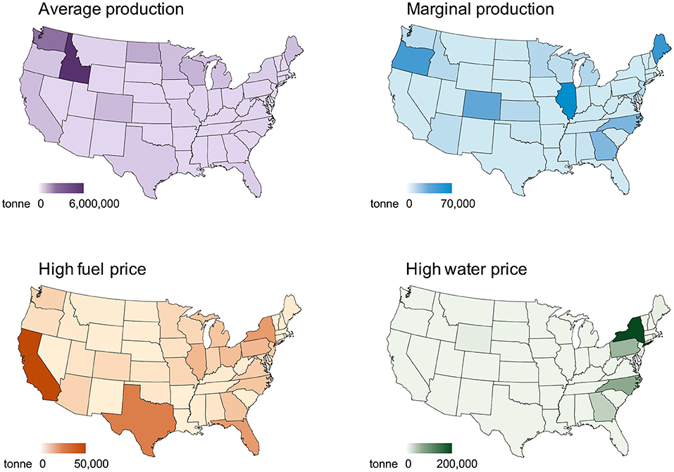
Figure 1. Maps of additional potato production under average production, marginal production, high fuel price, and high water price scenarios.

Under the high fuel price scenario, California (14%), Texas (9.8%), and New York (7.3%), and Florida (7.2%) would become the four top-producing states for the additional potato production to meet the recommended dietary of increased potato consumption. This pattern of marginal production was due to the population size of each state because high fuel price leads to more local production and supply than long-distance transportation. The production volume increases as population increases, for example, California and Texas. The average production pattern was close to the combination of marginal production and high fuel price scenarios: (1) northern states produce more potatoes than southern states do in general, and (2) states with larger populations like California and Texas produce more potatoes than states with smaller populations. Under the high water price scenario, the top producing states for marginal potato production were New York (43%), North Carolina (18%), Pennsylvania (16%), and Georgia (8.5%). This marginal production pattern was mainly caused by the irrigation water requirement for producing potatoes at the state level. Because less blue water was needed in the East Coast area than other states in the U.S., the potato production would be concentrated in those areas if water use minimization was the goal for policy-making.

Marginal Water Use Intensity

The weighted average blue water consumption for the additional production under the four production scenarios are presented in Figure 2. The results represent the weighted average national water use for one ton of marginal potato production based on the regional water use in the producing states. However, the weighted average results in the marginal and two policy scenarios should not be interpreted as linear factors. The water uses of additional demand are presented in Figure 3. The blue water intensity under the average production pattern was 96 m³ per ton of potato production. The water use intensity of marginal potato production was 68 and 66 m³ per ton under the marginal production and the high fuel price scenarios, respectively (29 and 31% lower than the average water use). Under the marginal production, California and Taxes where water use for potato production is relatively high compared with other states produce much less potato than the BAU, which significantly decreases the overall water use. Under the high fuel price scenario, eastern states which have sufficient rain and require less irrigation produce more potato than BAU, which reduces the overall water use. Potato production under the high water price scenario consumed the lowest amount of water, 26 m³ per ton, reducing 73% water use than BAU because the additional potatoes were produced in the states with low irrigation water consumption.

FIGURE 2

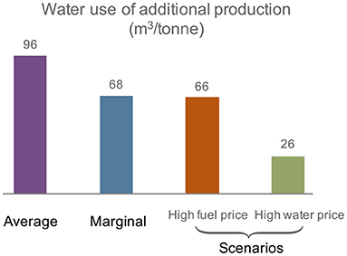
Figure 2. Weighted average water use for additional potato production under average production, marginal production, high fuel price scenario, and high water price scenario.

FIGURE 3

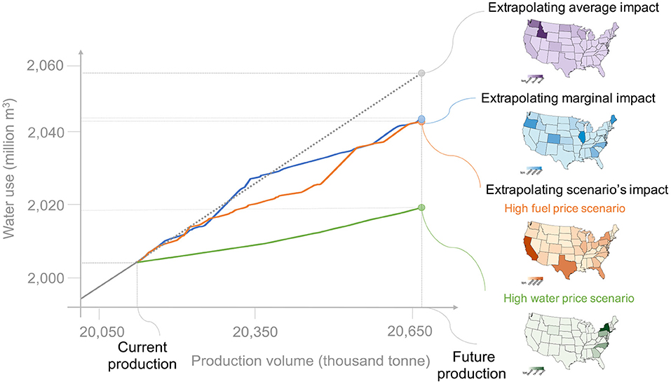
Figure 3. Water use for the current and the future potato production.

Total Water Consumption

The total water use in the average and marginal production for additional potatoes is shown in Figure 3. The water use of the current production volume is 2,006 million m³ per year. If we use the average production pattern to estimate future production, the water consumption of future potato production will follow a linear relationship as shown in the average impact in Figure 3. The cumulative water use for future production including the current and additional production would be 2,057 million m³ followed the current production pattern. However, the future production pattern would be different from the current production under marginal production and different policy goals. The total water use for the future production shows a non-linear relationship for marginal impact, high fuel price, and high water price scenarios, saving 16, 14, and 27 million m³ of water per year, respectively.

Conclusions and Discussion

Our study applied an optimization method, the transportation model, to estimate the marginal production and environmental stressor. This work demonstrated the transportation model method to predict blue water consumption using a numerical example of potato production to demonstrate the applicability. The case study used additional potato demand which USDA recommends as the marginal potato demand. The results indicate different environmental outcomes would be possible depending on how economic constraints, social factors, and policy measures play out. Unlike the majority of the LCA studies which use average values to linearly estimate marginal water use, the results using the transportation model show a non-linear relationship between marginal potato production and corresponding water use. Therefore, a “snapshot” of the current economic system as portrayed in LCA studies using average values falls short of addressing the question of dietary shift and supporting decision making.

Four production scenarios including the average, marginal, and two policy scenarios were analyzed in the study. Marginal production, high fuel price scenario, and high water price scenario reduced the marginal water use from the average production by 29, 31, and 73%, respectively. Our study indicates that marginal and alternative policy scenarios may lead to different policy outcomes than the average. Such marginal and policy scenario analysis can help understand the different pathways through which a decision may impact the economy and the environment.

The case study presented was meant to serve as an illustrative example. For more realistic results, it needs to be improved focusing particularly on the following key assumptions. The results from this analysis were based on the state-level data due to the data limitation of irrigation water use, and we assumed that potatoes would be delivered from the center of the producing state to the demanding state. We also assumed that the transportation fuel costs of transporting potatoes were proportional to the weight of potatoes excluding the case of unfilled trucks. Due to the lack of water use data for growing potatoes in some states, average water use data was applied to some states. The analysis didn't include the effect of dietary displacement and nutritional characterization that can be considered by future studies. In addition, we only considered fuel cost to represent transportation cost, which underestimated the actual transportation cost.

Our study only investigates the effect of additional potato demand on irrigation water use excluding the water use embodied in transportation, while other environmental stressors and more life cycle stages can be examined in future studies. We used cost minimization as the objective of the optimization model, but our method can be applied to other objectives such as minimizing greenhouse gas emissions and minimizing non-renewable energy consumption.

The method presented in the paper can be applied to spatially-explicit and scale-dependent modeling of other production systems in LCA involving multiple producers and consumers. Our model can be used to understand the non-linear behavior of marginal impacts over a change in demand. Future work might expand this method to assess other environmental impacts and test alternative policy scenarios. The development of regionally specific environmental data of crops is also crucial for improving the accuracy of the results and supporting optimal decision-making.

Data Availability Statement

The original contributions presented in the study are included in the article/Supplementary Material, further inquiries can be directed to the corresponding author.

Author Contributions

SS and SC proposed the framework. YQ performed the model calculation and analyzed the results. YY reviewed relevant literature. YQ, YY, and SS wrote the manuscript. All authors reviewed the manuscript, contributed to the article, and approved the submitted version.

Funding

This publication was developed under Assistance Agreement No. 83557901 awarded by the U.S. Environmental Protection Agency to University of California Santa Barbara. It has not been formally reviewed by EPA.

Disclaimer

The views expressed in this document are solely those of the authors and do not necessarily reflect those of the Agency. EPA does not endorse any products or commercial services mentioned in this publication.

Conflict of Interest

The authors declare that the research was conducted in the absence of any commercial or financial relationships that could be construed as a potential conflict of interest.

Acknowledgments

We are thankful to Dr. Adam Brandt for his valuable feedbacks and suggestions.

Supplementary Material

The Supplementary Material for this article can be found online at: https://www.frontiersin.org/articles/10.3389/frsus.2021.631080/full#supplementary-material

References

Aneja, V. P., Schlesinger, W. H., and Erisman, J. W. (2009). Effects of agriculture upon the air quality and climate: research, policy, and regulations. Environ. Sci. Technol. 43, 4234–4240. doi: 10.1021/es8024403

PubMed Abstract | CrossRef Full Text | Google Scholar

Boulay, A.-M., Benini, L., and Sala, S. (2020). Marginal and non-marginal approaches in characterization: how context and scale affect the selection of an adequate characterization model. The AWARE model example. Int. J. Life Cycle Assess. 25, 2380–2392. doi: 10.1007/s11367-019-01680-0

CrossRef Full Text | Google Scholar

Brandao, M., Martin, M., Cowie, A., Hamelin, L., and Zamagni, A. (2017). Consequential Life Cycle Assessment: What, How, and Why? Amsterdam: Elsevier.

Google Scholar

Bunch, S., Cort, K., Johnson, E., Elliott, D., and Stoughton, K. M. (2017). Water and Wastewater Annual Price Escalation Rates for Selected Cities Across the United States. Washington, DC: Off. Energy Effic. Renew. Energy.

Google Scholar

Campbell, B. M., Beare, D. J., Bennett, E. M., Hall-Spencer, J. M., Ingram, J. S. I., Jaramillo, F., et al. (2017). Agriculture production as a major driver of the Earth system exceeding planetary boundaries. Ecol. Soc. 22:8. doi: 10.5751/ES-09595-220408

CrossRef Full Text | Google Scholar

Conway, R. W., and Maxwell, W. L. (1961). A note on the assignment of facility location. J. Ind. Eng. 12, 34–36.

Google Scholar

Cooper, L. (1963). Location-allocation problems. Oper. Res. 11, 331–343. doi: 10.1287/opre.11.3.331

CrossRef Full Text | Google Scholar

Cucurachi, S., Yang, Y., Bergesen, J. D., Qin, Y., and Suh, S. (2016). Challenges in assessing the environmental consequences of dietary changes. Environ. Syst. Decis. 36, 1–3. doi: 10.1007/s10669-016-9589-2

CrossRef Full Text | Google Scholar

Dai, T., Yang, Y., Ross, L., Fleischer, A. S., and Wemhoff, A. P. (2020). Life cycle environmental impacts of food away from home and mitigation strategies-a review. J. Environ. Manag. 265:110471. doi: 10.1016/j.jenvman.2020.110471

PubMed Abstract | CrossRef Full Text | Google Scholar

Dixon, P. B., and Jorgenson, D. W. (2012). Handbook of Computable General Equilibrium Modeling. London: Newnes. Available online at: https://books.google.com/books?hl=enandlr=andid=F5WTcWLx4rMCandoi=fndandpg=PP1anddq=Handbook+of+Computable+General+Equilibrium+Modelingandots=BIrABLTmwIandsig=Ucj0cf5ze8ywPrY4kfcPppoEUIY (accessed February 14, 2016).

Google Scholar

Elzein, H., Dandres, T., Levasseur, A., and Samson, R. (2019). How can an optimized life cycle assessment method help evaluate the use phase of energy storage systems? J. Clean. Prod. 209, 1624–1636. doi: 10.1016/j.jclepro.2018.11.076

CrossRef Full Text | Google Scholar

Feldman, E., Lehrer, F. A., and Ray, T. L. (1966). Warehouse location under continuous economies of scale. Manag. Sci. 12, 670–684. doi: 10.1287/mnsc.12.9.670

CrossRef Full Text | Google Scholar

Ferguson, T. S. (2000). Linear Programming: A Concise Introduction. Available online at: http://www.math.ucla.edu/~tom/LP.pdf

Google Scholar

Forin, S., Berger, M., and Finkbeiner, M. (2020). Comment to “Marginal and non-marginal approaches in characterization: how context and scale affect the selection of an adequate characterization factor. The AWARE model example.” Int. J. Life Cycle Assess. 25, 663–666. doi: 10.1007/s11367-019-01726-3

CrossRef Full Text | Google Scholar

Garcia, D. J., and You, F. (2018). Addressing global environmental impacts including land use change in life cycle optimization: Studies on biofuels. J. Clean. Prod. 182, 313–330. doi: 10.1016/j.jclepro.2018.02.012

CrossRef Full Text | Google Scholar

Godfray, H. C. J., Aveyard, P., Garnett, T., Hall, J. W., Key, T. J., Lorimer, J., et al. (2018). Meat consumption, health, and the environment. Science 361:eaam5324. doi: 10.1126/science.aam5324

CrossRef Full Text | Google Scholar

Gong, J., and You, F. (2017). Consequential life cycle optimization: general conceptual framework and application to algal renewable diesel production. ACS Sustain. Chem. Eng. 5, 5887–5911. doi: 10.1021/acssuschemeng.7b00631

CrossRef Full Text | Google Scholar

Heijungs, R. (2020). The average versus marginal debate in LCIA: paradigm regained. Int. J. Life Cycle Assess. 26, 1–4. doi: 10.1007/s11367-020-01835-4

CrossRef Full Text | Google Scholar

Joshi, R. (2013). Optimization techniques for transportation problems of three variables. IOSR J. Math. 9, 46–50. doi: 10.9790/5728-0914650

CrossRef Full Text | Google Scholar

Kätelhön, A., Bardow, A., and Suh, S. (2016). Stochastic technology choice model for consequential life cycle assessment. Environ. Sci. Technol. 50, 12575–12583. doi: 10.1021/acs.est.6b04270

PubMed Abstract | CrossRef Full Text | Google Scholar

Low, S. A., Adalja, A., Beaulieu, E., Key, N., Martinez, S., Melton, A., et al. (2015). Trends in U.S. Local and Regional Food Systems. Washington, DC: US Department of Agriculture, Economic Research Service.

Google Scholar

Massey, M., O'Cass, A., and Otahal, P. (2018). A meta-analytic study of the factors driving the purchase of organic food. Appetite 125, 418–427. doi: 10.1016/j.appet.2018.02.029

PubMed Abstract | CrossRef Full Text | Google Scholar

Monge, G. (1781). Mémoire sur la théorie des déblais et des remblais: Histoire de 1'Academie Royale des Sciences.

Google Scholar

Mosier, A., Kroeze, C., Nevison, C., Oenema, O., Seitzinger, S., and van Cleemput, O. (1998). Closing the global N2O budget: nitrous oxide emissions through the agricultural nitrogen cycle. Nutr. Cycl. Agroecosyst. 52, 225–248. doi: 10.1023/A:1009740530221

CrossRef Full Text | Google Scholar

Mueller, N. D., Gerber, J. S., Johnston, M., Ray, D. K., Ramankutty, N., and Foley, J. A. (2012). Closing yield gaps through nutrient and water management. Nature 490, 254–257. doi: 10.1038/nature11420

PubMed Abstract | CrossRef Full Text | Google Scholar

Ongley, E. D. (1996). Control of Water Pollution From Agriculture. Rome: Food and Agriculture Organization of the United Nations.

Google Scholar

Palazzo, J., Geyer, R., and Suh, S. (2020). A review of methods for characterizing the environmental consequences of actions in life cycle assessment. J. Ind. Ecol. 24, 815–829. doi: 10.1111/jiec.12983

CrossRef Full Text | Google Scholar

Pimentel, D., and Pimentel, M. (2003). Sustainability of meat-based and plant-based diets and the environment. Am. J. Clin. Nutr. 78, 660S−663S. doi: 10.1093/ajcn/78.3.660S

PubMed Abstract | CrossRef Full Text | Google Scholar

Plevin, R. J., Delucchi, M. A., and Creutzig, F. (2014). Using attributional life cycle assessment to estimate climate-change mitigation benefits misleads policy makers. J. Ind. Ecol. 18, 73–83. doi: 10.1111/jiec.12074

CrossRef Full Text | Google Scholar

Qin, Y., and Horvath, A. (2020a). Use of alternative water sources in irrigation: potential scales, costs, and environmental impacts in California. Environ. Res. Commun. 2:055003.

Google Scholar

Qin, Y., and Horvath, A. (2020b). Contribution of food loss to greenhouse gas assessment of high-value agricultural produce: California production, US consumption. Environ. Res. Lett. 16:014024.

Google Scholar

Rajagopal, D., Hochman, G., and Zilberman, D. (2011). Indirect fuel use change (IFUC) and the lifecycle environmental impact of biofuel policies. Energy Policy 39, 228–233. doi: 10.1016/j.enpol.2010.09.035

CrossRef Full Text | Google Scholar

Roy, P., Nei, D., Orikasa, T., Xu, Q., Okadome, H., Nakamura, N., et al. (2009). A review of life cycle assessment (LCA) on some food products. J. Food Eng. 90, 1–10. doi: 10.1016/j.jfoodeng.2008.06.016

CrossRef Full Text | Google Scholar

Scott, A. J. (1970). Location-allocation systems: a review. Geogr. Anal. 2, 95–119. doi: 10.1111/j.1538-4632.1970.tb00149.x

CrossRef Full Text | Google Scholar

Springmann, M., Clark, M., Mason-D'Croz, D., Wiebe, K., Bodirsky, B. L., Lassaletta, L., et al. (2018). Options for keeping the food system within environmental limits. Nature 562, 519–525. doi: 10.1038/s41586-018-0594-0

PubMed Abstract | CrossRef Full Text | Google Scholar

Springmann, M., Godfray, H. C. J., Rayner, M., and Scarborough, P. (2016). Analysis and valuation of the health and climate change cobenefits of dietary change. Proc. Natl. Acad. Sci. U.S.A. 113, 4146–4151. doi: 10.1073/pnas.1523119113

PubMed Abstract | CrossRef Full Text | Google Scholar

Suh, S., Johnson, J. A., Tambjerg, L., Sim, S., Broeckx-Smith, S., Reyes, W., et al. (2020). Closing yield gap is crucial to avoid potential surge in global carbon emissions. Glob. Environ. Change. 63:102100.

Google Scholar

Suh, S., and Yang, Y. (2014). On the uncanny capabilities of consequential LCA. Int. J. Life Cycle Assess. 19, 1179–1184. doi: 10.1007/s11367-014-0739-9

CrossRef Full Text | Google Scholar

Tao, M., Adler, P. R., Larsen, A. E., and Suh, S. (2020). Pesticide application rates and their toxicological impacts: why do they vary so widely across the US?. Environ. Res. Lett. 15:124049.

Google Scholar

Tilman, D., and Clark, M. (2014). Global diets link environmental sustainability and human health. Nature 515, 518–522. doi: 10.1038/nature13959

PubMed Abstract | CrossRef Full Text | Google Scholar

Tilman, D., Fargione, J., Wolff, B., D'Antonio, C., Dobson, A., Howarth, R., et al. (2001). Forecasting agriculturally driven global environmental change. Science 292, 281–284. doi: 10.1126/science.1057544

PubMed Abstract | CrossRef Full Text | Google Scholar

Tilman, D., May, R. M., Lehman, C. L., and Nowak, M. A. (1994). Habitat destruction and the extinction debt. Nature 371, 65–66. doi: 10.1038/371065a0

CrossRef Full Text | Google Scholar

U.S. Department of Agriculture (2013). Estimated Quantity of Water Applied and Primary Method of Distribution by Selected Crops Harvested in the Open: 2013 and 2008. Washington, DC: USDA. Available online at: https://www.nass.usda.gov/Publications/AgCensus/2012/Online_Resources/Farm_and_Ranch_Irrigation_Survey/fris13_2_036_036.pdf (accessed December 20, 2018).

Google Scholar

U.S. Department of Agriculture (2015). Dietary Guidelines for Americans. Washington, DC: USDA. Available online at: https://health.gov/our-work/food-nutrition/2015-2020-dietary-guidelines/guidelines (accessed May 1, 2019).

Google Scholar

U.S. Department of Agriculture (2016a). Potatoes 2015 Summary. Washington, DC: USDA. Available online at: https://downloads.usda.library.cornell.edu/usda-esmis/files/fx719m44h/rx913s36b/fj236480z/Pota-09-15-2016.pdf (accessed May 15, 2019).

Google Scholar

U.S. Department of Agriculture (2016b). U.S. per Capita Loss-adjusted Vegetable Availability. Washington, DC: USDA. Available online at: http://www.ers.usda.gov/data-products/chart-gallery/detail.aspx?chartId=40071 (accessed January 6, 2019).

Google Scholar

U.S. Energy Information Administration (2019). Annual Energy Outlook 2019 With Projections to 2050. Washington, DC: EIA. Available online at: https://www.eia.gov/outlooks/aeo/pdf/aeo2019.pdf

Google Scholar

Vignaux, G. A., and Michalewicz, Z. (1991). A genetic algorithm for the linear transportation problem. Syst. Man Cybern. IEEE Trans. 21, 445–452. doi: 10.1109/21.87092

CrossRef Full Text | Google Scholar

Weber, C. L., and Matthews, H. S. (2008). Food-miles and the relative climate impacts of food choices in the United States. Environ. Sci. Technol. 42, 3508–3513. doi: 10.1021/es702969f

PubMed Abstract | CrossRef Full Text | Google Scholar

West, G. R. (1995). Comparison of input–output, input–output+ econometric, and computable general equilibrium impact models at the regional level. Econ. Syst. Res. 7, 209–227. doi: 10.1080/09535319500000021

CrossRef Full Text | Google Scholar

Willett, W., Rockström, J., Loken, B., Springmann, M., Lang, T., Vermeulen, S., et al. (2019). Food in the Anthropocene: the EAT–Lancet Commission on healthy diets from sustainable food systems. Lancet 393, 447–492. doi: 10.1016/S0140-6736(18)31788-4

PubMed Abstract | CrossRef Full Text | Google Scholar

Willkie, P. (2020). USDA Truck Rate Report. Washington, DC: USDA. Available online at: https://www.ams.usda.gov/mnreports/wa_fv190.txt (accessed April 20, 2019).

Google Scholar

Wilson, R., Klonsky, K., Sumner, D., Anderson, N., and Stewart, D. (2015). Sample Costs to Produce Potatoes. Davis, CA: University of California. Available online at: https://coststudyfiles.ucdavis.edu/uploads/cs_public/4e/f5/4ef54da3-114e-4952-a66a-049765b9a747/15potatofreshmktklamathfinaldraftdec10.pdf (accessed May 28, 2019).

Google Scholar

Yang, Y. (2016). Two sides of the same coin: consequential life cycle assessment based on the attributional framework. J. Clean. Prod. 127, 274–281. doi: 10.1016/j.jclepro.2016.03.089

CrossRef Full Text | Google Scholar

Yang, Y., and Campbell, J. E. (2017). Improving attributional life cycle assessment for decision support: the case of local food in sustainable design. J. Clean. Prod. 145, 361–366. doi: 10.1016/j.jclepro.2017.01.020

CrossRef Full Text | Google Scholar

Yang, Y., and Heijungs, R. (2018). On the use of different models for consequential life cycle assessment. Int. J. Life Cycle Assess. 23, 751–758. doi: 10.1007/s11367-017-1337-4

CrossRef Full Text | Google Scholar