Quantification of Non-linearities in the Consequential Life Cycle Assessment of the Use Phase of Battery Electric Vehicles

Introduction

The computational structure of matrix-based Life Cycle Assessment (LCA) is built on unit processes, which are in turn modeled as linear technologies, meaning that no effect of scale in production or consumption is conceived (Heijungs and Suh, 2002). However, this does not imply that computing the scaling vector components will result in linear equations (Heijungs, 2020). Moreover, non-linearities can be spotted in the impact assessment phase, too. Indeed, characterization factors represent partial derivatives obtained from models which are generally far from linear, such as the IPCC models for climate change (IPCC, 2013). Non-linear impact models may also be derived ex-post (Heijungs, 2020). In addition, non-linear dynamics in the Life Cycle Inventory (LCI) are always present, due to the inherent flows loops within the economy, but they become more relevant when such loops are contained in the foreground system. This is common in case studies on waste management and circular economy (Mclaren et al., 2000). Indeed, in Ekvall et al. (2007) it is acknowledged how the non-linear consequences of recycling rates on other inputs such as the fuel consumption for waste collection cannot be captured by traditional LCA studies. Nevertheless, functional unit-based LCA has the property of homogeneous linearity, meaning that there is a proportional relation between LCA results and the functional unit (Heijungs, 2020). In order to modify the underlying assumptions of unlimited supply of resources and intermediate products and properly account for economies of scale and further technological relationships, non-linear functions can be introduced within the conventional process LCA structure (Heijungs and Suh, 2002; Yang, 2017). However, introducing such modifications may not be necessary, as far as the conventional linear LCA model remains representative of the dynamics related to the studied product system (Yang, 2017).

This might not be the case for the LCI of electricity production, which might not scale linearly with the functional unit (Caduff et al., 2011; Bahlawan et al., 2019). Indeed, the technology mix that produces the electricity depends on the demand level (Lund et al., 2010; Brondi et al., 2019), it changes continuously, depending on the availability of wind and solar resources, and varies from region to region (Laurent and Espinosa, 2015; Cornago et al., 2020). Several studies addressed the specificity of electricity grid operation. They concluded that significant deviations of potential environmental impact reductions occur when adopting marginal and dynamic approaches instead of the conventional static linear LCA model, which is based on average values (Amor et al., 2014; Messagie et al., 2014). This is an important remark, as the contribution of electricity supply to LCA impacts is already crucial and the share of electricity in final energy consumption is expected to further increase (Vandepaer et al., 2019). Accordingly, several studies employed an energy system model (ESM) to enhance the accuracy of LCA results. Dandres et al. (2017) pointed out that the electricity grid operation may significantly change in response to the penetration of energy-intensive systems, such as data centers. Roux et al. (2017) modeled the complex interaction with the grid entailed by the newest buildings, due to demand control technologies. Both analyses concern with consequential LCAs at sectoral level, aiming at analyzing the changes induced by the introduction of a new system, which is able to influence the evolution of the electricity grid. This is in accordance to Mathiesen et al. (2009), who outlined the need to perform sensitivity analyses across different scenarios through ESM in order to correctly identify a complex set of marginal energy technologies in consequential LCAs.

A similar context concerns with the penetration of Electric Vehicles (EVs) in the transport sector. EVs already accounted for 2.6% of the 2019 global car sales and are projected to constitute 31% of the 2040 global vehicle fleet, with Battery Electric Vehicles (BEVs) accounting for most of EVs (BloombergNEF, 2020; IEA, 2020). Policies are motivated by the lower environmental impacts associated to EVs (IEA, 2020), which are also outlined by a relevant report at the European level (Ricardo, 2020). Such projected EV growth is expected to influence the evolution of electricity grids toward more interconnected systems (Das et al., 2020). In addition, different studies pointed out a significant potential for reduction of excess electricity production from renewables through coordinated charging of EV (Richardson, 2013; Jian et al., 2017; Mehrjerdi and Rakhshani, 2019). Moreover, the variability of marginal electricity productions is recognized to be a key factor to reduce the use phase impacts of BEV and other electricity-shifting policies (Graff Zivin et al., 2014). Coherently, such interest lead to more than 80 studies in the LCA field for the only BEV technology, which is also found to show the best performance among EVs (Ricardo, 2020). However, an accurate modeling of electricity used to charge EVs is only included by a limited number of studies, with many publications employing a ready-to-use dataset instead (Girardi et al., 2015). This is a crucial shortfall, as potential environmental impacts of EVs are strongly affected by electricity supply (Doucette and McCulloch, 2011; Nordelöf et al., 2014; Cox et al., 2020; Ricardo, 2020), which is found to explain 70% of the variability of the resulting EV carbon intensity (Marmiroli et al., 2018). Such variability also depends on the interaction of the EVs fleet with the electricity system and EVs charging profile (Girardi et al., 2015; Rangaraju et al., 2015). Accordingly, Marmiroli et al. (2018) indicated that adopting a vehicle-level point of view and linearly upscaling the related results with EV penetration rate would not capture fleet-level dynamics, thus it would be questionable, in addition to not being recommended by LCA standards (EC-JRC, 2010). However, in addition to the model developed within (Ricardo, 2020), few fleet-based LCAs on EVs have been developed. Bohnes et al. (2017) evaluated different scenarios of EV diffusion in the urban area of Copenhagen, while Girardi et al. (2015) accounted for the interdependence between EV and electricity grid. However, none of them investigated how LCA results of different EV penetration scenarios may change, due to the interdependence with the electricity grid. The present study focuses on this gap, with a 3-fold aim.

Firstly, we introduce three possible approaches, which progressively include BEV-specific dynamics, for improving the LCI model of a BEV, by explicitly including the interaction between the use phase of the fleet with the electricity grid within the foreground system. BEVs are chosen to represent all EVs, due to both their promising environmental performances and their higher electricity intensity (Ricardo, 2020). Both the electricity system and the BEVs fleet are modeled with the EnergyPLAN ESM. EnergyPLAN is an input/output deterministic bottom up model that aims to identify optimal energy system designs and operation strategies looking at the complete energy system. It is based on a series of hourly simulations over a 1-year time period (Lund, 2014). Such model employs a sufficiently high temporal resolution; thus it is able to couple BEVs demand variations with electricity grid dynamics, induced e.g., by weather conditions, especially for regions with a high installed capacity of renewable electricity technologies. This work is contextualized within the Italian country, which is of particular interest due to the diversity of its electricity producing technologies.

Secondly, we evaluate and quantify the occurrence of non-linearities in the LCA results due to five levels of BEVs market penetration in 2030. The evaluation of new technologies diffusion at large scale, additional to a Business-As-Usual (BAU) scenario calls for a consequential LCA approach (EC-JRC, 2010; Dandres et al., 2017).

Thirdly, we aim to discuss how the high time resolution and the BEV charge profiles that are computed within EnergyPLAN can provide a more accurate assessment of the marginal LCA impacts, in accordance to the indications of Girardi et al. (2015), and may be a further source of non-linearity in the LCA results. Variations of LCA results across the three approaches for marginal LCI modeling are discussed.

This analysis leads to the set-up of a new methodological framework, that can be used to include sources of non-linearities in the LCA of BEV, to obtain more robust conclusions to support decisions and policies at the meso/macro level scale (Sala et al., 2016).

Materials and Methods

This section is organized into three parts. The first subsection outlines the scope of the study. The second subsection provides a methodological focus on the LCI, related to the calculations of marginal long-term electricity mixes. The third subsection provides an insight on the data used for simulating the Italian energy system with EnergyPLAN, in order to facilitate the interpretation of results.

Scope of the Study

The analyzed product system is constituted by a fleet of BEV passenger cars, which are operated in Italy across their useful life. Plug-in Hybrid Electric Vehicles (PHEV) and hybrid electric vehicles are thus excluded from the study. The functional unit of the study is related to the marginal provision of 1 km transport service by BEV passenger cars. As a starting point, the generic cradle-to-grave dataset “transport, passenger car, electric” from the ecoinvent 3.6 consequential database was considered. Within such dataset, the process related to electricity consumed in BEV use phase constitutes the foreground system of this study, which is refined according to the ESM results. To enhance the interpretation of results, a specific focus is devoted to an intermediate functional unit, as made in Ricardo (2020): i.e., the electricity consumed in the use phase of such system. Firstly, our study analyzes the provision of 1 kWh of low voltage electricity in Italy. Secondly, the supply of the yearly electricity demand associated to the entire BEVs fleet is discussed. Thirdly, the variations of the distributions of hourly LCA impacts associated to the provision of 1 kWh of electricity are shown. Eventually, the variations of LCA results of 1 km transport by BEV, due to the explicit foreground LCI model of use-phase electricity are discussed.

The ESM is chosen coherently with the aims of the study: EnergyPLAN employs an hourly time resolution over a year, while keeping a relatively simple and aggregated structure. The model is able to integrate projections and historical data collected and developed by national research institutes, such as Terna and GSE in the Italian case. Moreover across this study, indications on the Italian national energy strategy are drawn from the “Integrated National Energy and Climate Plan,” which is the latest set of policies submitted to the European Commission in 2019 (Piano Nazionale Integrato Energia e Clima, PNIEC) (MiSE et sl., 2018). The ESM analyses are developed starting from Marmiroli's work (2020).

Concerning LCI modeling, the consequential, long-term approach is adopted. In the foreground system, the electricity process is analyzed in terms of its structural response to changes, being it modeled as a mix of long-term marginal processes. According to the goal of the study, a BAU scenario for 2030 in Italy must be chosen. The most recent studies at the Italian level outline that the current market trend is projected to lead to a range of 1.8–2 million EVs (Enel European House Ambrosetti, 2017; Energy Strategy group, 2018). At the policy level, the PNIEC considers incentives for spreading low-emission passenger vehicles, yet without providing any specific target on expected shares of passenger EVs. Since our analysis only includes BEVs, which do not constitute the totality of EVs, the lowest value of 2030 EVs penetration rate, according to the presented projections, is chosen to represent the BAU scenario. Therefore, we assume that PNIEC objectives include the diffusion of 1.8 million BEVs, which constitutes the BAU scenario. Data on electricity production by source for 2016 and 2030 BAU scenarios are, respectively, collected in accordance to the PNIEC.

Concerning product system boundaries, the useful life of the car modeled in the cited ecoinvent dataset is deducted to be 150,000 km, according to the indications on car weight. This dataset has a global geographical coverage, meaning that its LCI processes are determined through the use of global market mixes. In the present analysis, the geographical coverage of the only use phase is modified, contextualizing it within the Italian country. Within the use phase, the only electricity provided for operating BEVs is included in the foreground system, as it is the only process with both a reasonable dependence on the country in which the vehicle is operated and a noticeable relevance in determining LCA impacts for BEVs. The background system includes production, maintenance, road and wear-related emissions, and End-of-Life (EoL) processes related to BEV; therefore, such system is not changed in this study. Concerning time boundaries, the ecoinvent 3.6 consequential database computes yearly marginal electricity mixes using 2030 as the time horizon year and 2015 as reference year (Vandepaer et al., 2019). The same approach is followed here, yet 2016 is chosen as reference year due to data availability.

Within this framework, five scenarios with different 2030 BEVs diffusion levels into the Italian passenger car fleet are implemented. In accordance to the goal of the study, to show the potential occurrence of non-linearities in LCA results, the penetration of BEVs into the Italian passenger car fleet is modeled up to 100% with a stress test, with 4 steps of 25% each. According to Capros et al. (2016), the size of the European passenger car fleet is not expected to grow from 2016 on. Thus, the absolute level of the Italian passenger car fleet is kept equal to the 2016 value, i.e., 38 million cars (ACI, 2017). Therefore, BEVs constitute 4.75% of the entire fleet in the BAU scenario, while the additional four scenarios model a fleet which is constituted by 25, 50, 75, and 100% BEVs. The last 3 cases are purely speculative, as such values are not reached even in the most optimistic scenarios developed within (Enel European House Ambrosetti, 2017; Energy Strategy group, 2018).

The selected Life Cycle Impact Assessment (LCIA) method is ILCD 2.0 midpoint, as such method is designed for policy decision support (Sala et al., 2012). The selection of the most relevant impact categories for this study is based on three criteria. Firstly, since the focus of the study is related to the Italian marginal electricity mix, the relevance of LCIA results for this process, relative to the cradle-to grave LCIA results, is evaluated. Secondly, the relevance of BEV LCIA results with respect to global impacts is accounted for. Thirdly, a selection within LCIA categories which are similarly influenced by variations of the Italian marginal electricity mix is carried out. Figure 1 focuses on the first two criteria: it shows the normalized BEV LCIA results, grouped by relevant providers, for the “transport, passenger car, electric” ecoinvent dataset, modified using Italian electricity provider for BEV operation. Figure 1 shows that the most relevant LCIA categories for the present analysis can be Non-carcinogenic effects, Carcinogenic effects, Minerals and metals, Climate change total, Freshwater eutrophication, Freshwater ecotoxicity, and Fossils. However, it was observed that LCIA trends for the Fossils and Freshwater ecotoxicity categories are, respectively, similar to Climate change total and Freshwater eutrophication (see Supplementary Figures 7–9), thus according to the third criterion, these categories are not considered. Finally, Respiratory effects, inorganics is included in the study, as it is indicated to be relevant in the Product Environmental Footprint Category Rules (PEFCR) for batteries (Siret et al., 2018), thus it may be important as well for the present study. Selection of impact categories would not have changed if the final results for the electricity dataset were considered: section Additional Discussion of the Supplementary Material provides additional discussion on the selection of impact categories. Moreover, section Outputs of the Supplementary Material provides LCIA results for all the ILCD impact categories.

FIGURE 1

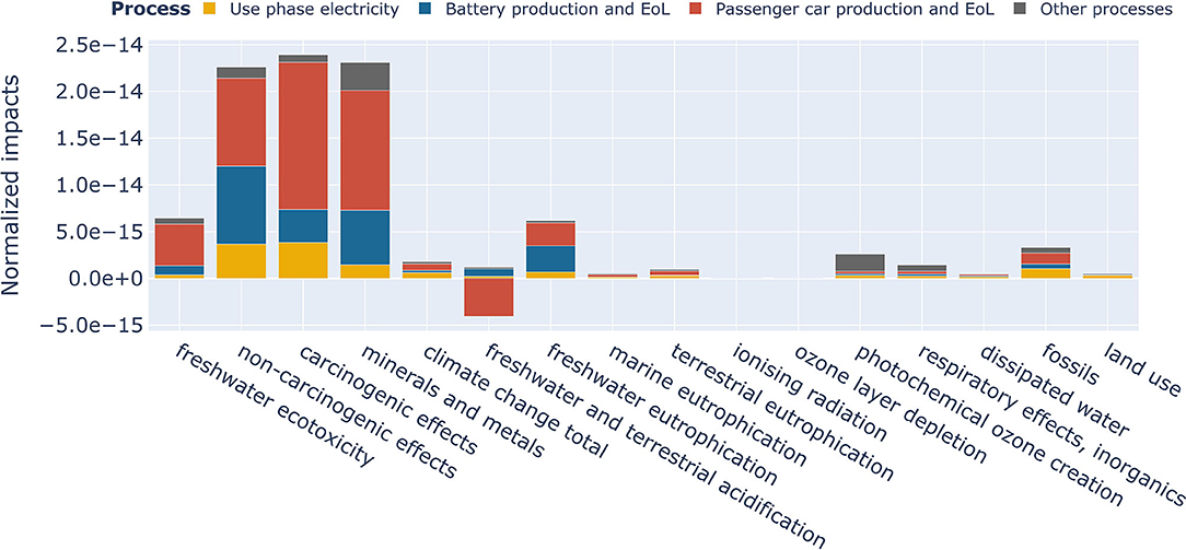
Figure 1. LCIA results for the “transport, passenger car, electric” dataset, modified using the Italian electricity provider for BEV operation, from ecoinvent 3.6 consequential database, grouped by relevant LCI processes, normalized according to global PEFCR factors (Siret et al., 2018), for the different ILCD midpoint 2.0 LCIA categories.

LCI Methodological Setup

The present analysis overall requires six ESM simulations to be built: the first is related to historical 2016 data, while the remaining are related to the five 2030 scenarios of BEVs diffusion. Then, marginal electricity mixes for each of the five 2030 scenarios are computed.

Recalling the first aim of the study, three different approaches for computing marginals are here presented, representing three different levels of detail that may be used in LCA for BEV. The first approach computes marginal electricity mixes at the yearly level, while the second one additionally involves the hourly time resolution employed by EnergyPLAN. Finally, the third approach even includes BEV hourly charging profiles. The three approaches are named according to the temporal resolution of marginal electricity productions used to compute them and to the weighting of mixes to account for BEV charging curves, whenever this is performed. Marginal mixes computed through equation 1 are referred to as Yearly. Marginal mixes computed through equation 2 are called Hourly. Eventually, marginal mixes computed through equation 4 are named Hourly weighted, since they account for a weighting process based on BEV charging profiles.

Recalling the second aim of the study, results from the above presented approaches are compared with the conventional linear LCA approach, which is here represented by the use of the ecoinvent 3.6 consequential dataset for the Italian electricity mix. Accordingly, this approach is named Ecoinvent. The ecoinvent long-term consequential system model aims at reflecting long-term consequences of small-scale decisions. Such decisions do not influence key market parameters, thus they are assumed to linearly scale with the size of the related change (Vandepaer et al., 2019). Instead, our analysis investigates the variation of such key market parameters and the consequent occurrence of non-linearities, which are thus quantified in contrast with the Ecoinvent approach. In addition, a comparison with the Ecoinvent approach can outline the relevance of underlying data sources used to compute marginal electricity mixes, as the Italian ecoinvent dataset is derived from European reference scenarios (Vandepaer et al., 2019), differently from our study, as section Modeling of Energy Scenarios outlines.

Eventually, given the third aim of the study, the differences between the 3 BEV-dependent marginal mixes are outlined, too.

The first approach, Yearly, employs Equation 1, presented in Vandepaer et al. (2019), for computing marginal electricity supply shares with respect to 2016, across the five 2030 scenarios:

$\begin{array}{ll}{S}_{i,2030}=\frac{P_{i,2030}-P_{i,2016}}{{\displaystyle {\sum }_i^n\left(P_{i,2030}-P_{i,2016}\right)}}& (1)\end{array}$

With i being each of the n unconstrained electricity production technologies, P being the quantity of electricity produced within the related year by technology i, S being the share of technology i in the considered marginal supply mix. Unconstrained electricity production technologies do not include electricity produced in Combined Heat and Power (CHP) mode, as in that case electricity is produced as a secondary product. Whenever the numerator of the equation is negative, S is given the value of 0 (Vandepaer et al., 2019).

The Yearly approach does not consider that even if the eventual P_{i, 2030} is lower than P_{i, 2016}, some technologies may increase their hourly electricity production in 2030, with respect to 2016, across some hours of the year. Thus, stating that a specific electricity production technology is not included in the yearly marginal electricity mix may not be fully true. Section Modeling of Energy Scenarios outlines that for Italy, the 2030 electricity demand is projected to be higher than the 2016 one, but P_{natural gas, 2016} is equal to 126 TWh (GSE, 2018), while the projected P_{natural gas, 2030} is equal to 118 TWh (MiSE MATTM, 2017). Consequently, S_{natural gas, 2030} is null. However, whenever the 2030–2016 increase in electricity demand is not covered by Variable Renewable Electricity Sources (VRES) (i.e., during hours with a low solar irradiation or wind), thermal power plants must cover such increase, thus leading to a positive marginal electricity production within specific hours of the year, as will be shown by Figure 2. The second approach, Hourly, aims at filling this gap using Equation 2:

$\begin{array}{ll}{S}_{i,2030}=\frac{{\displaystyle {\sum }_h^{8784}\left(P_{i,h,2030}-P_{i,h,2016}\right)}}{{\displaystyle {\sum }_h^{8784}\left({\displaystyle {\sum }_i^n\left(P_{i,h,2030}-P_{i,h,2016}\right)}\right)}}& (2)\end{array}$

With h being the considered hour of the year. The same approach was followed by Lund et al. (2010), who computed a long-term yearly average marginal technology based on hourly dynamics. EnergyPLAN employs 8,784 h, even if 2030 is not a leap year. However, whenever hourly distributions are required (e.g., electricity demand, VRES productions), the 2016 distributions are employed for 2030 as well, as a matter of consistency between scenarios. Section Electricity System Specifications and Additional Discussion of the Supplementary Material, respectively, provide explanations and motivations on the use of data distributions within EnergyPLAN.

FIGURE 2

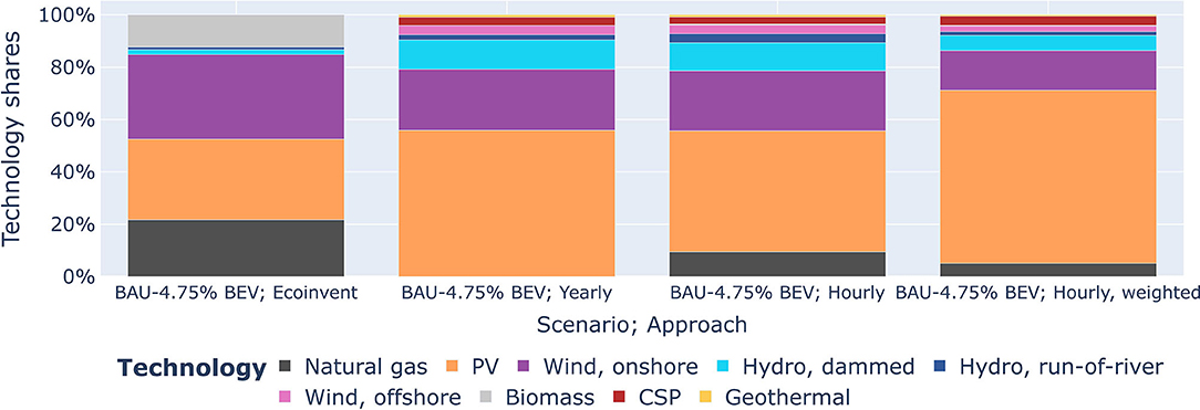
Figure 2. Marginal electricity mixes in the BAU scenario computed with the four different approaches.

Still, the Hourly shares do not consider the charging patterns of BEVs, i.e., what the actual electricity consumed by BEVs is. Thus, we propose a third method for calculating marginals, based on the indications of Girardi et al. (2015). Therefore, we introduce W_h, which is defined by Equation 3 and is used to weigh the hourly electricity marginal productions on the charging profiles of BEVs:

$\begin{array}{ll}{W}_h=\frac{C_h}{{\displaystyle {\sum }_i^n\left(P_{i,h,2030}-P_{i,h,2016}\right)}}& (3)\end{array}$

With C_h being the amount of electricity which is used to charge the BEVs fleet. The denominator of the equation represents the total hourly marginal electricity production. Then, the Hourly, weighted approach employs Equation 4 to obtain aggregated shares which are representative of the actual electricity consumed by our product system:

$\begin{array}{ll}{S}_{i,2030}=\frac{{\displaystyle {\sum }_h^{8784}\left(P_{i,h,2030}-P_{i,h,2016}\right)\ast W_h}}{{\displaystyle {\sum }_h^{8784}{C}_h}}& (4)\end{array}$

Finally, in accordance to the ecoinvent database, all the electricity production terms P_i and P_i,h are computed according to the consumption mix of the country. Due to the penetration of VRES, Excess Electricity Production (EEP) may arise in the ESM simulation. EEP must be either exported or curtailed, thus it is not actually consumed within the country. Consequently, it had to be subtracted from the electricity mix. Hence, the theoretical electricity production P_{2030,theoretical} related to each of the VRES technologies is decreased, according to the values of EEP for the related time step (yearly in case of equation 1 and hourly in case of Equations 2 and 4). The subtraction term shown by Equations 5 and 6 is weighted on the relative electricity production of each of these sources in the considered time interval. Electricity production from Concentrated Solar Power (CSP) is decreased, too. This technology has the possibility to store thermal energy and it may theoretically allow for a higher degree of flexibility of electricity production. However, CSP is still not mature in the Italian market, thus as a conservative hypothesis, this technology is assigned no stabilization property of the grid. Equation 5 is performed at the yearly level and applies to the P_i term of equation 1, for both 2016 and 2030 years:

$\begin{array}{ll}{P}_{i,year}=P_{i,year,theoretical}-EE{P}^{*}\frac{P_{i,year,theoretical}}{{\displaystyle {\sum }_i^5{P}_{i,year,theoretical}}}& (5)\end{array}$

With i ranging from 1 to 5, which is the number of VRES technologies included within such assessment, i.e., onshore and offshore wind, solar photovoltaic (PV) and CSP, run-of-river hydro. Equation 6 is instead performed at the hourly level, according to the EnergyPLAN outputs:

$\begin{array}{ll}{P}_{i,year}={\displaystyle \sum _h^{8784}(P_{i,h,year,theoretical}-EE{P}_h^{\ast }\frac{P_{i,h,year,theoretical}}{{\displaystyle {\sum }_i^5{P}_{i,h,year,theoretical}}})}& (6)\end{array}$

In order to obtain the LCI and LCIA results related to every scenario, the computed long-term electricity production mixes are inputted to the high and low voltage electricity mix datasets for Italy of the ecoinvent 3.6 consequential database, thus changing the related LCI through the brightway2 software (Mutel, 2017).

Modeling of Energy Scenarios

Within this subsection, the only data that are key to understand the Results and Discussion sections are presented. A full assessment of the entire energy system of Italy is not related to the aims of the paper, since focus is devoted to the only electricity system. On the demand side, we updated the values of total electricity demand and import/exports, together with explicitly modeling BEVs demand. On the supply side, the electricity production data by source are computed. The evolution of heating and cooling supply by means of technologies which run on electricity, e.g., electric heating and cooling or CHP, is not explicitly modeled here: the related data are kept fixed to the 2016 levels and are discussed in section EnergyPlan of the Supplementary Material, together with additional information on EnergyPLAN technical parameters and equations.

Our analysis overall requires six ESM simulations. The outputs of 2016 simulation are used both as reference for calculating marginals and for calibration of EnergyPLAN outputs. Concerning the 2030 scenarios, the installed capacities of different technologies are computed on the BAU projections of electricity production, according to the PNIEC objectives. Such capacities are not changed across 2030 scenarios. This means that reduced RES curtailment and thermal power plants are assumed to cover the additional BEVs electricity demand across scenarios. Section Discussion of Model Assumptions discusses the motivation behind this assumption and related implications.

Additional information used to model the 2030 BAU scenario is based on the projections elaborated by RSE (2017) for the National Energy Strategy (MiSE MATTM, 2017), which was elaborated in 2017 to create a favorable context for the PNIEC adoption. Quantitative targets of PNIEC that are of interest for this study are the phase out of coal by 2025, together with the 2030 share of RES in electricity production and in the supply of transport demand, which must, respectively, reach 55.4 and 21.6%. The PNIEC policies are estimated to lead to a 36% reduction of greenhouse gases emission from car transport, with respect to 2005, which is mostly due to the electrification of this sector, rather than to biofuels penetration (MiSE et sl., 2018).

EnergyPLAN offers the possibility to perform either a technical analysis, which implements different technical simulation strategies, or a market exchange analysis, which works on the optimization of business-economic profits for each plant (Lund and Thellufsen, 2020). Due to the difficulty in predicting energy prices, a technical simulation strategy is set up. A discussion on the robustness of this analysis is provided in section Discussion of Model Assumptions. Required EnergyPLAN inputs are related to energy demands, production capacities, efficiencies and energy sources. The outputs consist of annual energy production balances, which are then used to compute LCI marginals as described in section LCI Methodological Setup.

All electricity data are here expressed in gross terms, since this is the actual electricity produced. Grid electricity losses are accounted for as in the original ecoinvent dataset. Losses and modeling of hydroelectric pump operation are explained in section Inputs of the Supplementary Material.

Demand

The 2016 electricity production is 325 TWh (MiSE et sl., 2018), with a net import of 37 TWh (GSE, 2018). Still according to the PNIEC, the electricity demand in 2030 is expected to be 337 TWh, while the net import value decreases with respect to 2016 and is expected to be 29 TWh. The hourly distributions of total electricity demand and imports are downloaded from the national transmission system operator (Terna, 2020). Transmission line capacity, used by EnergyPLAN to compute additional imports/exports is set to 0, as imports and exports are exogenously fixed.

Concerning BEVs electricity demand, the amount of EVs in Italy during 2016 is 5743 (both PHEV and BEV) (Marmiroli, 2020). As simplifying hypothesis, such vehicles are modeled as BEVs. A yearly mileage per vehicle of 11,000 km/year (Energy Strategy group, 2018) is assumed, together with an electricity consumption of 0.199 kWh/km, which is in accordance to the employed ecoinvent dataset and similar to the values indicated by Girardi et al. (2015). The resulting electricity demand is thus 2.19 MWh/y/vehicle, which results on 0.013 TWh/y for the entire 2016 fleet. The grid-to-battery efficiency for both 2016 and 2030 is estimated to be equal to 90%, in accordance to the EnergyPLAN models developed in Connolly et al. (2015). Therefore, the resulting required supply of electricity is 2.43 MWh/y/vehicle, corresponding to an electricity demand from the grid of 0.014 TWh/y. Consequently, assuming the same efficiency values and yearly mileage of 2016, the demand for BEVs transport increases as Table 1 shows.

TABLE 1

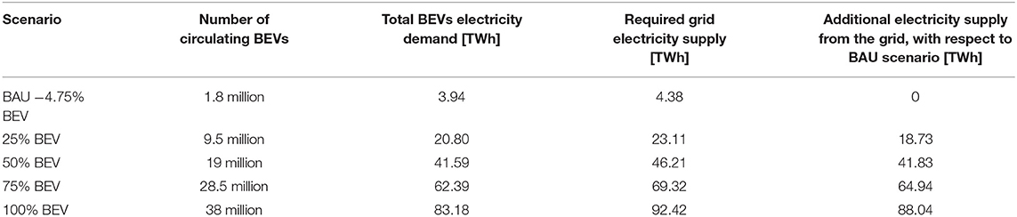
Table 1. BEVs features in the future scenarios for 2030.

The projected amount of electricity demand for BEVs in the 25% scenario constitutes around 6% of the 2030 total electricity demand, which would be equal to 356 TWh in such scenario. This is in accordance with (Terna, 2018), which estimated that electricity demand from EV would at most be equal to 5% of the total in the most aggressive scenario that is developed in that report (27% EV in the national fleet).

Concerning the charging infrastructure of BEVs, the model allows to differentiate between Dump and Smart Charge setting. The Dump Charge is modeled as a traditional uncontrolled plug-in charge, in which the user recharges the battery whenever it is needed. With the Smart Charge, on the other hand, battery charging is used aiming to decrease excess electricity production. Such demand for 2016 is modeled with the Dump Charge setting, while for the future 2030 scenarios, BEVs diffusion is modeled with the Smart Charge. Additional specifications on BEV modeling parameters and implications of our choices are, respectively, discussed in section Battery Electric Vehicles (BEVs) Specifications and Additional Discussion of the Supplementary Material.

Supply

The review provided by Marmiroli (2020) outlines that in Italy, future additional generation capacity will mainly consist of RES, with PV having the highest increase potential, to fill the gap left by coal phase out. Hydroelectric power plants capacity will not change dramatically, as most of the suitable sites are already exploited.

With the technical simulation strategy of EnergyPLAN, within each hour, VRES are given priority of production, as well as electricity production from geothermal sources and CHP. The latter technology is set up to only follow the demand for heat, producing electricity as a byproduct, which is consistent with considering it a constrained electricity production technology in the ecoinvent consequential dataset for electricity production, as section LCI Methodological Setup outlined. CSP and dammed hydroelectric power plants are then operated in order to firstly best utilize the natural input and secondly minimize EEP. Then, reversible hydro power (i.e., pumped hydro) is activated in order to reduce EEP and the amount of BEVs Smart Charge is computed. Only after these steps, if still either the demand is higher than the supply or grid stabilization requirements must be fulfilled, electricity production from thermal power plants is computed.

Table 2 shows VRES electricity productions, which are drawn from the PNIEC, apart from CSP estimated production, which is derived from the Italian national energy strategy. Moreover, the specification of 2030 offshore wind electricity production is based on PNIEC indication of projected capacity (900 MW) and on the indications by IEA (2019), which state that new offshore wind plants currently show capacity factors of 40–50%. Concerning hydroelectric power plants, investments will be focused on increasing the usage of hydro storage and they will be mainly focused on big size plants (MiSE MATTM, 2017; MiSE et sl., 2018). The additional 2030 electricity production from hydroelectric sources is equal to 3.1 TWh, but no indication was found on how such increase should be divided between run-of-river and dammed plants. Therefore, we equally divide the increase by these 2 sources, shown in Table 2. The 2016 total hydroelectric production, without pumped is equal to 46.2 TWh and it is selected from (MiSE et sl., 2018), while 2016 shares between run-of-river and dammed hydro are derived from Terna (2016).

TABLE 2

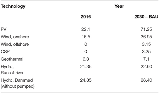
Table 2. Electricity production [TWh] from RES (biomass excluded). Historical data for 2016 and projected data for 2030 according to PNIEC objectives.

As will be seen in the Results section, marginal electricity derived by dammed hydro power results to be much higher than 1.55 TWh due to additional water charging linked to pumped hydro storage plants operation. The related modeling is explained in section Inputs of the Supplementary Material. We specified BAU in the 2030 column heading because electricity production from VRES is not fixed across scenarios: it increases in response to higher BEVs demand, due to better exploitation of EEP.

Concerning thermal power plants, EnergyPLAN requires fuel shares data, which are not changed across the possible two operating modes of these plants. Indeed, thermal power plants may produce both heat and electricity (CHP mode) or electricity only (condensing mode). Historical 2016 data on total (condensing + CHP) power production by source are collected from GSE (2018). CHP electricity production is collected by Eurostat, 2019) and is assumed to not change until 2030, due to unavailability of projections. Electricity production in condensing mode is computed by subtracting electricity production in CHP mode from the total amounts of electricity by source. Electricity production from thermal power plants for the BAU scenario is calibrated on the National Energy Strategy model (MiSE MATTM, 2017). Fuel shares do not change across the remaining 2030 scenarios, while electricity production from these sources increases in response to BEVs demand, which is why we specified BAU to the 2030 column heading in Table 3 as well. Section Thermal Power Plants Electricity Supply of Supplementary Material thoroughly describes assumptions lying behind Table 3 values.

TABLE 3

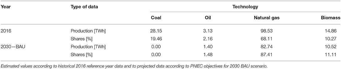
Table 3. Electricity production and fuel distributions of central thermal power plants (geothermal excluded), in condensing mode.

Results

This section is divided into three parts, which present the outcomes of our analysis, with discussions of drivers and implications to facilitate interpretation. The first two subsections are focused on the intermediate functional unit of the study, i.e., the provision of electricity, while the third one discusses the variation of LCIA results related to the cradle-to-grave LCA for BEVs.

The first subsection focuses on LCI results across the four approaches. LCI results in the BAU scenario are firstly shown and then, the variability of electricity mixes across scenarios is assessed. Such discussion is preliminary to the second subsection, which analyzes the deviations of LCIA results, computed through the 4 approaches, across the 5 scenarios. Such section introduces to which degree accounting for the spreading of BEVs may influence results, both in terms of unitary LCIA results (i.e., per kWh of electricity produced) and in terms of total LCIA results (i.e., marginal potential impacts associated to the entire BEVs fleet). Then, variations of hourly impacts distributions across scenarios and the related implications across the presented approaches are discussed, addressing the third aim of the study. Finally, the third subsection highlights how cradle-to-grave BEV impacts vary across the selected 6 impact categories, due to the variation of the only use-phase electricity LCI.

Technology Shares

Figure 2 shows the marginal electricity mixes of the BAU scenario, resulting from the four approaches outlined in section LCI Methodological Setup. The Yearly approach leads to a mix with a strongly lower share of fossil fuels, with respect to the Ecoinvent one. Indeed, neither natural gas nor biomass condensing power plants increase their yearly production with respect to 2016, as can be clearly seen by Table 3. The Yearly mix is therefore dominated by PV and wind, which account for more than 80% of it. Instead, the Hourly mix appears to be more similar to the Ecoinvent one, with a natural gas fueled plants share of 9.50%, which appears because they operate during hours in which RES electricity production cannot satisfy the additional hourly demand. Finally, the Hourly, weighted mix still shows the presence of natural gas, yet with a smaller contribution with respect to the Hourly marginals. The share of PV is instead higher, since BEVs charging is privileged across the central hours of the day, as Figure 4 will further discuss. Furthermore, the share of hydro, dammed is nearly halved with respect to the Hourly approach. Indeed, as section Modeling of Energy Scenarios explained, when EEP arises, EnergyPLAN decreases dammed hydroelectric power production and instead, water storages are charged by means of pumps.

Then, Figure 3 shows the variability of marginal electricity mixes across the analyzed scenarios, for the 3 non-linear approaches followed in this study. The Ecoinvent shares are not shown here, as they do not vary across scenarios. Due to our hypothesis of keeping VRES capacities constant across scenarios, the general trend is related to the increase of natural gas share to match additional BEV electricity demand. Such increase occurs more steeply across the Yearly marginals, in which the share of natural gas increases from 0% in the 25% BEV scenario to 32.79% in the 100% BEV scenario. Indeed, positive EEP amounts of 12.68 and 3.69 TWh appear, respectively, in the BAU and 25% BEV scenarios. Thus, according to our hypotheses, within the BAU and the 50% BEV scenarios, the increase in BEVs electricity demand is partly covered by EEP exploitation and partly by thermal power plants. This is why the Yearly marginal electricity production from natural gas condensing power plants in the 25% BEV scenario is still not positive (see Supplementary Table 4). From the 50% BEV scenario on, the increase in BEVs electricity demand is only covered by thermal power plants (mostly natural gas, with small contributions of biomass, as can be inferred by Table 3 shares) in condensing mode. This results in an increase in the derivative of the curve related to the natural gas share, which occurs from 25% BEV to 75% BEV scenarios. This variation of derivative is much more evident for the Yearly marginals, since the Hourly and Hourly, weighted approaches account for the dynamics of electricity production within a year, which smooth the increase of natural gas electricity production. From 75% BEV to 100% BEV scenarios, the derivative of the curve related to natural gas share decreases again. The Hourly, weighted marginals show the peculiarity of a steep increase of natural gas share already in the 25% BEV scenario and the related derivative does not decrease when moving toward the 100% BEV scenario, in which the highest natural gas share across the analyzed approaches is reached, being it equal to 38.94%.

FIGURE 3

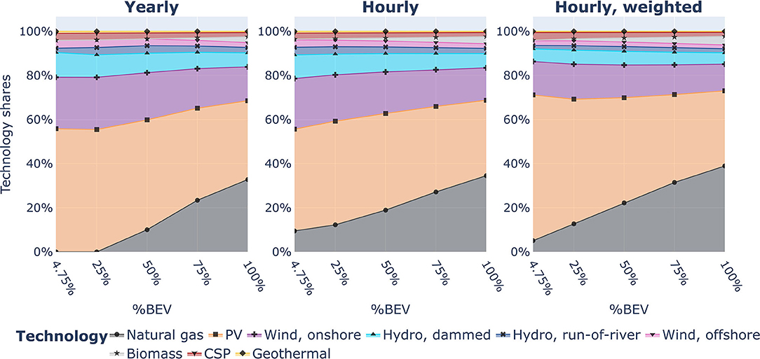
Figure 3. Marginal electricity mixes across scenarios, computed with the three non-linear approaches.

To facilitate the interpretation of the Hourly, weighted LCI results, Figure 4 outlines the interdependence between the distribution of BEVs charge profiles, which are related to the weights W_h, and the variation of average hourly electricity mixes across scenarios. Supplementary Figures 2, 3 provide the full variation of both quantities across scenarios. Hourly charge values are shown as a fraction of the electricity charged in the related day, to clearly outline the contribution of each hour.

FIGURE 4

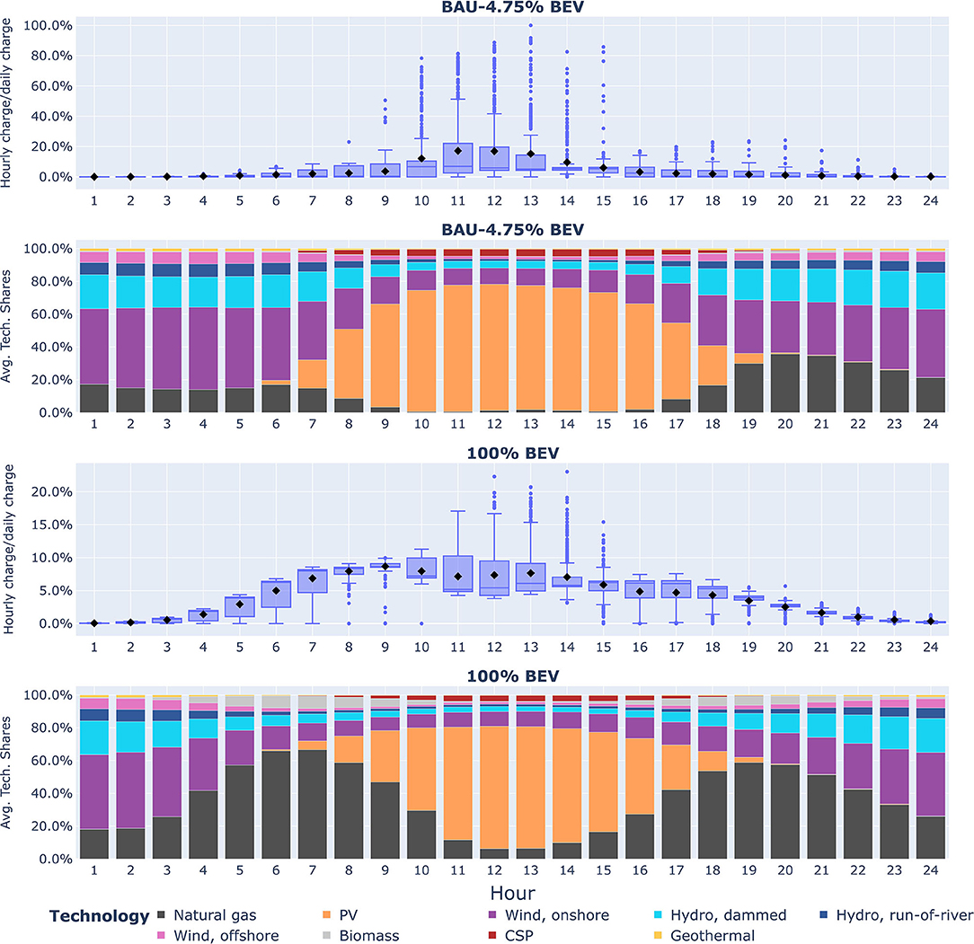
Figure 4. Distributions of the different 366 hourly charge profiles, relative to daily charge, with black markers representing average values, coupled with average hourly marginal electricity mixes. Both charts are shown for the BAU and 100% BEV scenarios. In the x-axis, hour 1 refers to the first hour of the day and the same happens for other values.

The distribution of 366 hourly charge profiles results from both the transport demand curve, taken from the EnergyPLAN models developed in Connolly et al. (2015) and the choice of Smart Charge simulation, which stimulates charging when EEP is produced. Even if the distribution of transport demand is fixed across scenarios, distributions of hourly electricity consumed for BEVs charging do change, as the absolute value of transport demand changes with the size of the BEVs fleet, too. Indeed, the BAU and 100% BEV scenarios show strongly different distributions. The distribution of BEVs charge profiles in the BAU scenario shows many outliers, which are due to the EnergyPLAN model seeking to fully exploit electricity produced by PV and CSP. Solar energy is highly relevant in the 2030 Italian mix and is more available within the central hours of the day, differently from other RES. EnergyPLAN applies the same logic to wind energy exploitation, which is responsible for outliers that are not within the central hours of the day. In the BAU scenario, BEVs transport demand is very low and EEP is high, therefore charging occurs mainly to reduce EEP. Conversely, moving toward the 100% BEV scenario, the relevance of BEVs on the total electricity demand increases, thus BEVs are charged also within other hours of the day, which are not necessarily those in which EEP may occur. Hence, additional BEVs make the charging curve flatter and looking more similar to the transport demand curve (see Supplementary Figure 2), with all the 100% BEV ordinates being lower than 25% in Figure 4. Moreover, from the 50% BEV scenario on, EEP is null, thus additional electricity demand is mainly covered by natural gas, which starts penetrating even in the central hours of the day. In particular, Figure 4 shows that the penetration of natural gas especially affects early morning and evening hours. Indeed, night shares do not significantly change across scenarios, as the charging process mainly happens within the day. This means that the increase in electricity demand happens within hours in which solar VRES cannot adequately respond. Therefore, the higher the BEVs diffusion, the higher the contribution of thermal power plants in charging additional BEVs. This trend is fully captured by the Hourly, weighted approach only, as confirmed by the related increase in natural gas share across scenarios in Figure 3. Hence, our hypothesis of keeping the same VRES capacities across different scenarios has particularly significant implications especially on the actual electricity consumed by BEVs.

Impact Analysis

All the trends outlined in section Technology Shares are reflected onto the related LCIA impacts. The unitary impacts per kWh of marginal electricity, related to the BAU scenario mixes outlined by Figure 2, are shown in Table 4. Then, Figure 5 shows the trends of unitary impacts, relative to the values of BAU scenario with the Hourly, weighted approach. Such representation allows to outline which impact categories are mostly affected by the variation of shares across scenarios and methodological approaches. The Ecoinvent trend is constant, as this approach cannot account for interactions between the electricity LCI and the BEVs fleet.

FIGURE 5

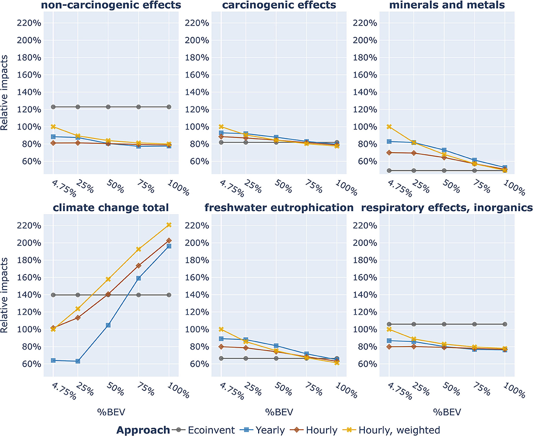
Figure 5. Unitary impacts associated to the provision of 1 kWh of marginal electricity supply, for the 6 selected LCIA categories and the four approaches, across the analyzed scenarios. Values are relative to the BAU scenario impacts computed with the Hourly, weighted approach.

TABLE 4

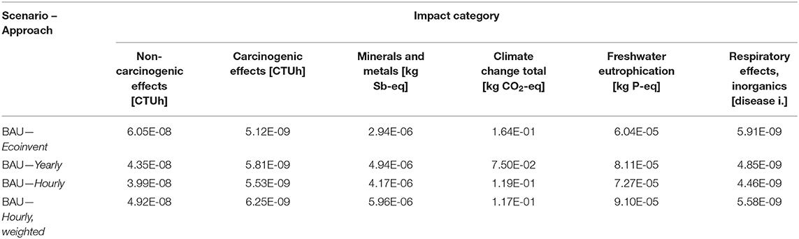
Table 4. Unitary impacts per kWh of marginal electricity supply, for the 6 selected LCIA categories and the four approaches, associated to the BAU scenario.

Carcinogenic effects is the least affected impact indicator, with the curves related to all the 4 approaches being confined within the 80–100% interval. The opposite happens for Climate change total indicator, in which the 3 non-linear curves span across an interval of 60–220%. In the BAU scenario, results for the Ecoinvent approach differ by +39.74% for the Climate change total category and by −49.27% for Minerals and metals category, with respect to the BAU, Hourly, weighted value. Thus, employing different approaches for marginal calculations is a significant source of variability of LCIA indicators. These two categories also show the greatest variations of non-linear curves, as they are strongly dependent by the balance between RES and fossil fuels shares within the electricity mix, due to the unitary impact of each technology (see Supplementary Figure 5). Apart from the Climate change total charts, the difference within the 3 non-linear curves decreases when moving toward the 100% BEV scenario. Indeed as Figure 3 showed, the higher the BEVs demand, the higher the penetration of natural gas. Therefore, within the same scenario and across the 3 non-linear approaches, the differences of shares related to other technologies decrease. Apart from Climate change total, impact indicators are dominated by technologies other than natural gas, thus we see that the 3 non-linear curves progressively approach each other. For instance, the Minerals and metals impact indicator is dominated by PV penetration: the lower the differences in PV shares, the lower the differences in Minerals and metals impacts across the 3 non-linear approaches. Indeed, starting from a 50% wide range, the different curves converge into a very narrow range in the 100% BEV scenario.

The Climate change total indicator computed with the Yearly approach is highly sensitive to the increase of BEVs, as a consequence of the highly variable shares outlined by Figure 3. On the other hand, the Hourly curve shows instead the smoothest trends across LCIA categories, while the opposite holds true for the Hourly, weighted results. Regarding this category, the Hourly and Hourly, weighted curves start from very close values in the BAU scenario, despite the latter having a much smaller share of natural gas in the electricity mix, as shown by Figure 2. This happens because the BAU mix for the Hourly, weighted curve also shows a much smaller share of electricity from hydro, dammed with respect to the same scenario for the Hourly curve. Hydro, dammed electricity is one of the cleanest sources of electricity production within this category, with unitary impacts being one order of magnitude lower than electricity from PV (see Supplementary Figure 5). Moreover, the trend of non-linear curves within this impact category reflects the penetration of natural gas within the marginal electricity supply mix, with a steep growth from 25% BEV to 75% BEV scenario, followed by a decreasing derivative within the 75% BEV and 100% BEV scenarios.

It must be remarked that according to our model, Climate change total is the only category which is negatively affected by higher penetration of BEVs. However, the relative variations of other categories across the 5 scenarios are much smaller. Within the Climate change category, moving from the BAU to the 100% BEV scenario, all the 3 non-linear curves double their unitary impacts.

Across the 6 impact categories, the ranges defined by the 4 curves in the BAU scenario are strongly different with respect to those related to the 100% BEV scenario. For instance, in the Climate change total category, the BAU scenario values range from 60 to 140%, while the 100% BEV scenario values span across 140–220%. Figure 6 shows how this aspect is translated into the LCIA indicators associated to the total marginal electricity demand evolution across additional fleets of BEVs. Such curves are obtained by multiplying the unitary impacts by the yearly electricity demand per vehicle (see section Demand) and by the number of additional BEVs associated to each scenario. From the comparison with the Ecoinvent values, it is evident how linearly upscaling marginal impacts with the number of circulating BEVs (i.e., what would be done with a conventional LCA employing the Ecoinvent approach, or in general employing the only BAU unitary impact indicators) would lead to significant non-linearities, as unitary impacts are found to vary across scenarios, especially for the Climate change total category. Indeed, the linear Ecoinvent approach leads to an underestimation of 8.35 Mton CO₂-eq in the 100% BEV scenario for the Climate change total category, with respect to the Hourly, weighted results. Similarly, linearly scaling the Hourly, weighted results keeping the BAU unitary impact would lead to an underestimation of 12.45 Mton CO₂-eq with respect to the case in which the interaction with the electricity grid is accounted for. In accordance with Figure 5, non-linearities are especially significant for the Climate change total and Minerals and metals category, while this is not the case for the remaining impact categories. Total impacts for penetration of additional BEVs are null in the BAU, as no additional BEV is present in this scenario.

FIGURE 6

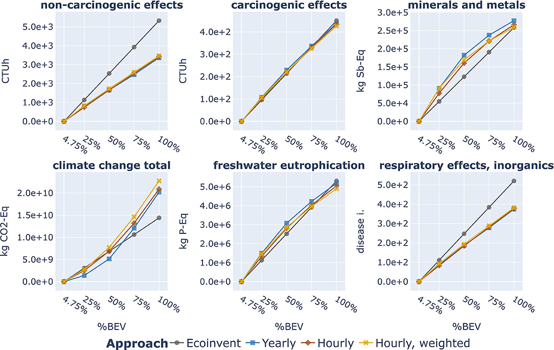
Figure 6. Absolute impacts associated to the provision of the total electricity supply requested by the marginal BEV fleet, for the 6 selected LCIA categories and the four approaches, across the analyzed scenarios.

The last result of this section highlights again the capabilities provided by an ESM. Impacts computed with the mixes derived by Equations 2 and 4 are related to an aggregation at the yearly level of 8,784 hourly mixes. Shares defined with the Hourly approach can be stated to weight the hourly electricity mixes by the related amount of marginal electricity production. That is, the higher the marginal electricity production related to a specific hour, the higher the influence of such hour in determining S_{i, 2030}. Shares defined by the Hourly, weighted approach are instead weighted on the BEVs electricity charge of each hour. Given the LCA methodology structure, the weighting process may be done either with mixes (at the LCI level) or with impacts (at the LCIA level). Figure 7 stresses out that the Hourly and Hourly, weighted curves are the result of both an underlying hourly impact distribution, which varies across scenarios, and an aggregation process, which varies across the two approaches and clearly constitutes a source of deviations between aggregated LCIA results. If different BEVs charge profiles were assumed, not only the aggregation of the Hourly, weighted approach would change, but also the underlying distribution would be different, especially at higher number of circulating BEVs: see section Contextualization Within the Literature.

FIGURE 7

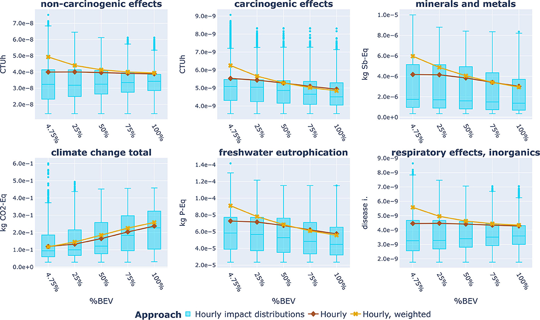
Figure 7. Distributions of hourly unitary impacts and aggregated values computed with the Hourly and Hourly, weighted approaches, associated to the provision of 1 kWh of marginal electricity supply, for the 6 selected LCIA categories, across the analyzed scenarios.

Distributions of hourly impact indicators for the BAU scenario appear to be asymmetrical, with the presence of outliers in the upper part of the charts. This is due to the high EEP in the BAU scenario, which makes the productions of VRES decrease (see Equations 5 and 6) and is generally linked to the activation of both natural gas, for grid stabilization requirements (see section 1.1.1 of the Supplementary Material) and the hydro pump technology, which makes unitary impacts further increase (see section Inputs of the Supplementary Material). Accordingly, the higher the number of BEVs, the more the distributions are symmetrical and less outliers are shown. Carcinogenic effects show a large number of outliers, due to high unitary impacts of wind and solar technologies (see Supplementary Figure 5), which are also the most relevant VRES across marginal mixes. Respiratory effects, inorganics shows the presence of outliers in the BAU and 100% BEV scenario. For the former scenario, the reason lies behind high presence of PV in the mix, which shows the second higher unitary impact in this category. For the latter scenario, the reason lies behind the presence of biomass in the mix, which shows the highest unitary impact in this category.

Minerals and metals distributions yet remain strongly asymmetrical. Given that impacts within this category are dominated by PV (see Supplementary Figure 5), the shape of this distribution can be inferred to be related to the presence of sunny days. It is reasonable that 50% of the distribution is instead confined within a small interval (lower than 2e-6 kg Sb-eq), because these values are related to night hours.

Contextualization Within LCA Results for BEVs

This subsection shows how the variability of the use phase electricity LCI makes the cradle-to-grave LCIA results vary. As in the previous section, Table 5 shows the unitary impacts associated to the provision of 1 km of transport service by passenger electric car in the 4 BAU scenarios. Then, Figure 8 shows the trends of unitary impacts, relative to the values of BAU scenario with the Hourly, weighted approach.

TABLE 5

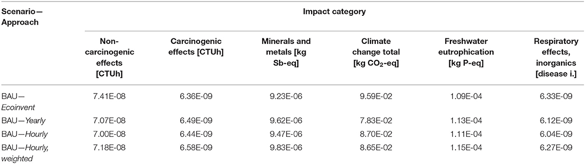
Table 5. Marginal unitary impacts associated to the provision of 1 km of transport service by BEV car in the BAU scenario, for the 6 selected LCIA categories and the four approaches.

FIGURE 8

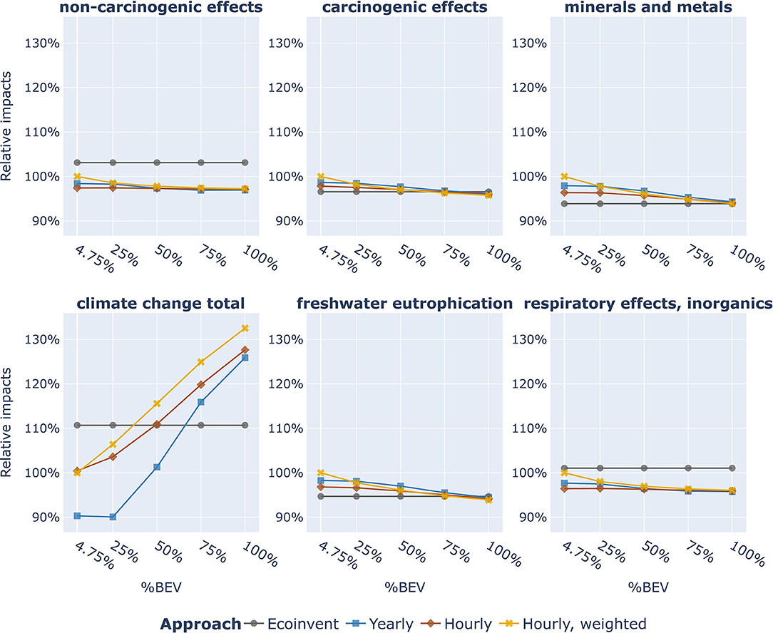
Figure 8. Marginal unitary impacts associated to the provision of 1 km of transport service by BEV passenger car, for the 6 selected LCIA categories and the four approaches, across the analyzed scenarios. Values are relative to the BAU scenario impacts computed with the Hourly, weighted approach.

In addition to what section Impact Analysis showed, Figure 8 outlines that the variability of BEV LCA results depends on the relative importance of the electricity process within each of the analyzed impact categories, which can be inferred from Figure 1. Accordingly, even if the electricity process shows a high variability within the Minerals and metals category, Figure 8 shows that the variation of impacts for 1 km of electric transport is within an interval of 10% across the analyzed curves. Indeed, the contribution to impacts of car and battery production processes dominate within this category. LCIA indicators related to Carcinogenic effects and Freshwater eutrophication show a very low variability, due to both low variability of use phase electricity-related impacts and a low relevance of this process within BEVs results. In particular, Minerals and metals and Freshwater eutrophication show an average 6.1% decrease of the Hourly, weighted unitary impacts, across the two extreme scenarios. Within Non-carcinogenic effects and Respiratory effects, inorganics, the differences between the 3 curves is lower than 5%, as well as the deviation with respect to the BAU scenario. This is definitely not the case for the Climate change total category, in which a range of 90.31–110.70% is defined for the BAU scenario across the 4 curves. Moreover, for the Hourly, weighted curve, the 100% BEV scenario shows a 32.52% higher impact with respect to the BAU scenario. Concerning the Yearly plot, the variation is even higher, spanning from 90.31 to 125.90% across the analyzed scenarios, i.e., +39.40% total increase. Therefore, within this category, moving toward high numbers of circulating BEVs, the electricity process becomes more and more dominant in determining the impacts of 1 km BEV transport (see Supplementary Figure 6). The Hourly, weighted curve shows the highest variations between the BAU and the 100% BEV scenarios, which are on average equal to 9.28% across LCIA categories.

Discussion

The present section aims at contextualizing the main results obtained in section Results within the literature and discuss assumptions and limitations of the study, in order to eventually provide indications for including our methodological framework within comprehensive assessments of entire transport systems for policymaking support.

Subsection Contextualization Within the Literature discusses key findings of the study, contextualizing them into the literature, with a comparison of previous analyses results. The influence of assumptions that are implied within the current study and by the use of EnergyPLAN are discussed in subsection Discussion of Model Assumptions. Then, methodological indications on the inclusion of the evaluation of non-linearities are drawn in subsection Methodological Indications.

Contextualization Within the Literature

The present study coupled the indications of Girardi et al. (2015), which accounted for the interdependence between EV and electricity grid, with the evaluation of different scenarios of EVs diffusion as made in Bohnes et al. (2017) and Ricardo (2020). Bohnes et al. (2017) did not account for changes in the electricity grid operation due to BEVs penetration into the market. They assumed that potential increases of electricity demand could be counterbalanced by efficiency gains in EV. Moreover, their study is focused on an urban area, while our study is related to the country level. We did not consider counterbalancing factors, as we aimed to model relevant interactions with the electricity system, which may occur as outlined by other studies (Girardi et al., 2015; Ricardo, 2020). Girardi et al. (2015) considered energy prices dynamics within his model, which is not the case in this study. In Ricardo (2020), an attributional approach is followed, yet some consequential elements are modeled, too. These are related to the additional electricity demand from EV, economies of scale and decarbonization of production processes over time. Table 6 provides a summary of similar studies that can be compared with the present one, i.e., analyses related to future BEVs.

TABLE 6

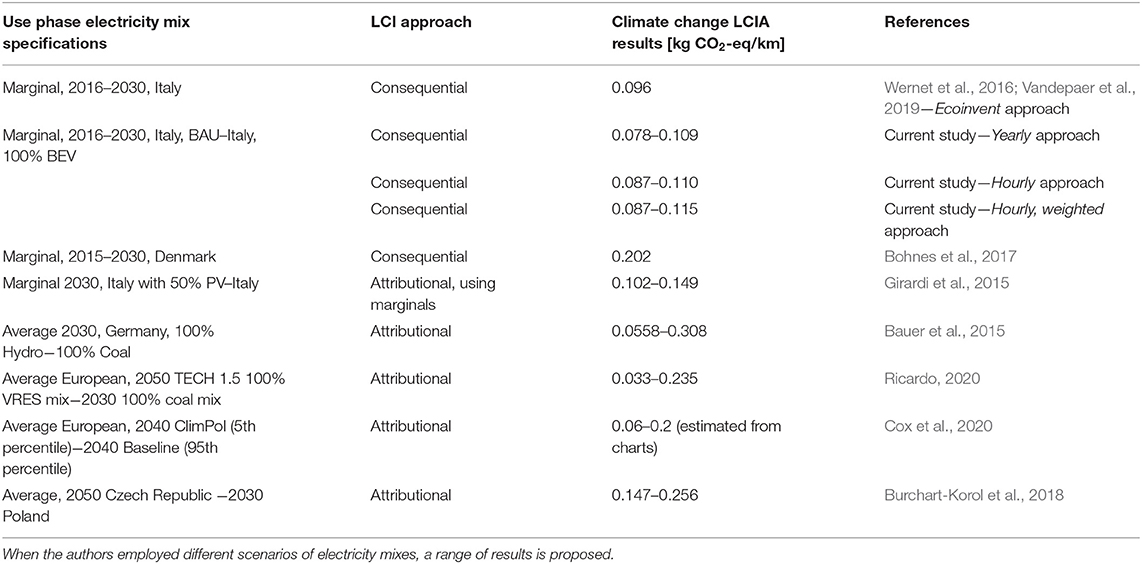
Table 6. LCIA results of the current and previous studies on future passenger car BEVs penetration which assumed 2030 or further as time horizon, for the Climate change total category.

In addition to the presented results, Huo et al. (2015) evaluated average fuel-cycle emissions for 2025 BEVs operation, finding values between 0.060 and 0.170 kg CO₂-eq/km, respectively, for China BTR and U.S. NPCC regions. Our results are in line with Girardi et al. (2015), especially for the case in which BEVs are charged by electricity produced for 50% by PV. Using the Italian 2030 marginal mix, Girardi et al. (2015) found a much higher result compared to our BAU scenario. This is due to the assumption of the 2030 model employed by that study, which considers BEVs electricity demand as an additional demand, which will be covered by thermal power plants only, assuming that RES are already fully used. This is true for Bauer et al. (2015) as well, which further outlines how BEVs results are influenced by the employed electricity mix. The results found by Burchart-Korol et al. (2018) are also in line with this considerations, as the Polish 2030 electricity mix is constituted by 80% fossil fuels. Bohnes et al. (2017) found a relatively high value of BEVs Climate change result, which is due to retaining a share of coal in the marginal electricity mix and to the higher electricity demand of BEVs. In Ricardo (2020), a sensitivity analysis on electricity chain assumptions over different time spans is performed. Such analysis shows the lowest value of Table 6, due to the larger time span (2050), hypothesis on decarbonization of production processes and a strongly clean electricity mix. Similarly, Cox et al. (2020) integrated 2040 electricity scenarios from integrated assessment models into the ecoinvent database, assessing variations of both the use phase electricity mix and of production processes. Moreover, such study also employed a Monte Carlo global sensitivity analysis for all performance parameters of the assessed EVs. The same authors already assessed such scenarios within a previous study (Cox et al., 2018) which leads to similar considerations, concerning Climate change impacts of future BEVs, thus it was not added to Table 6. Both the TECH 1.5 and the ClimPol scenarios model the implementation of European climate targets. The variability of our results is correctly lower compared to Bauer et al. (2015), Huo et al. (2015), Burchart-Korol et al. (2018), Cox et al. (2020), and Ricardo (2020), which assessed highly variable electricity mixes.

In Mathiesen et al. (2009) and Lund et al. (2010), it is demonstrated that long-term marginal electricity supply cannot be constituted by a single technology only and the determination of such mix requires ESM simulations. Indeed, they stated that affected technologies depend both on the geographical location and on the temporal resolution of the study, especially at higher shares of fluctuating renewable energy sources, analyzing the Danish electricity system. Our study validates such considerations for the Italian context too, as it shows that noticeable differences between the Yearly and Hourly approaches, which, respectively, neglect and account for hourly electricity system dynamics. Moreover, we also show the relevance of the different approaches on LCA results for BEV transport services, further validating the need to perform complex analyses for product systems in which energy supply is a relevant process, as stated in Mathiesen et al. (2009). Furthermore, our study highlights that the LCI of electricity supply is strongly sensitive to the amount of marginal electricity demand (see the variations across scenarios of BEV penetration), and to employing the latest policy indications (see the variations between Ecoinvent and Yearly approaches). Thus, we agree with (Mathiesen et al., 2009; Lund et al., 2010) on the need to perform a scenario analysis, in order to avoid that the LCA results become obsolete due to changes in marginal electricity supply mix. Finally, the literature suggested that the actual electricity used to charge BEVs, which depends on the charging profile and on the interaction with the grid, must be accounted for in order to provide accurate LCA results (Nordelöf et al., 2014; Girardi et al., 2015; Rangaraju et al., 2015). In our study, the Hourly, weighted approach shows significant variations of LCIA results across scenarios. In our model, such variations are indeed related to the variability of the actual electricity consumed by BEVs across scenarios, which are not fully captured by other approaches. Therefore, we confirm the literature indications, as we find that accounting for BEVs charging profiles constitutes an additional source of non-linearities in LCIA results. Hence, we estimate that Hourly, weighted is the most accurate approach in accounting for non-linearities, too.

Discussion of Model Assumptions

The 2030 BAU scenario is modeled accounting for the system response to current policies, detailed in the PNIEC, in accordance to the consequential, long-term point of view (see section Modeling of Energy Scenarios). However, our LCI model relies on the assumption that no additional RES capacity is installed to cope with the additional BEVs demand across the different scenarios. Thus, no response, in terms of additional installed capacity, of the 2030 system with respect to the 4 additional scenarios with different levels of circulating BEVs is modeled. Hence, the system response to BEVs which are additional with respect to the BAU scenario is a short-term one, as such response is only constituted by the variation of electricity production (Marmiroli et al., 2018). Accordingly, LCI differences across scenarios are mostly due to natural gas penetration, as shown by Figure 3. Another way to build the LCI model could have been to increase RES installed capacity, in order to be able to meet PNIEC objectives given the BEVs transport demand increase. However, even in this case, in the BAU scenario, the differences between the 4 analyzed approaches would emerge again, as they are not affected by this hypothesis. Changing this hypothesis, we would observe a lower penetration of natural gas in the LCI of marginal mixes across scenarios, which would in turn affect especially the LCIA results of the Climate change total indicator. Only for this category, we estimate that the variability of LCIA results across scenarios would probably decrease. The results of other LCIA categories are instead mainly driven by single RES technologies (e.g., PV is the main driver of Minerals and metals results). Thus, they would vary according to which RES capacities increase and consequently, several different trends may appear. However, changing our main hypothesis would lead to additional problems.

Firstly, adding further hypotheses on additional RES installed capacity for each of the analyzed 2030 scenarios, apart from the BAU one. This means deciding on which type of RES is installed and it would lead to lower reproducibility. Moreover, capacity may not be strongly increased for all RES, as for instance hydroelectric capacity is already almost saturated in Italy (MiSE et sl., 2018).

Secondly, a technical simulation strategy is chosen within EnergyPLAN, thus excluding the dynamics of energy prices. Moreover, the energy system is modeled as if it constituted a single market zone. This is not true for Italy, which is constituted by 6 market zones (Gestore Mercati Energetici, 2020). Moreover, EnergyPLAN explicitly models neither frequency regulation nor inertia within the energy system and the BEVs fleet is modeled as if it was a single battery (Lund and Thellufsen, 2020). Thus, with the current EnergyPLAN setup, we are not able to distinguish whether BEVs demand is generated in the South or in the North of Italy. Moreover, determining accurate BEVs demand distributions at the national scale is challenging, since the actual location of every BEV matters, in determining whether there are sufficient charging stations in a specific area. Grid stabilization requirements are only managed through a specific parameter (see section Electricity System Specifications of the Supplementary Material). This means that simulating strongly different systems, with respect to the 2030 reference one, with the current set up of EnergyPLAN would not lead in any case to more accurate results.

Accordingly, particular attention must be devoted to the geographical context of the study. The country electricity mix is one of the most impacting parameters in the sensitivity analysis performed by Ricardo (2020), even if differences across countries will be lower over the years due to the progressive decarbonization of electricity systems. Within our study, BEVs are charged during the day to reduce EEP and to better use the available solar energy, as captured by the BAU results of the Hourly, weighted approach. However, this is a country-specific result, as it depends on the projected strong reliance of Italy on solar energy. If BEVs were operated in France, which mostly runs on nuclear power, daily BEV charging is likely to not lead to a higher exploitation of solar energy. Another example is constituted by Denmark, which is expected to increase its RES share mostly by means of wind power (Bohnes et al., 2017), which may be available during the night too, thus it has different dynamics than solar power. The general remark is that BEV charging should enable a higher RES exploitation, i.e., when RES are available in the specific area of the study, if the objective is to reduce BEVs carbon footprint. Concerning the geographical scale of the analysis, it may make sense to model high diffusions of BEVs at a smaller scale than the national one. BEVs have the potential to decrease urban air pollution (IEA, 2020) and several studies focused on BEVs diffusion at the city scale (Bohnes et al., 2017; Jian et al., 2017).

Another aspect of interest is related to the BEV charge profiles. Figure 4 outlined that charging BEVs during hours in which VRES cannot provide additional electricity, has particularly strong implications on natural gas usage, since thermal power plants would be the main source of electricity which can adequately respond to such demand. Indeed, the average electricity mixes related to early morning and evening hours are the most affected by additional electricity demand. If different BEVs charge profiles were assumed, or the Smart Charge simulation was not chosen, not only the aggregation of the Hourly, weighted approach would change, but also the underlying distribution (see Figure 7) would be different, especially at higher number of circulating BEVs. If for instance, BEVs were charged during the night, two main effects would happen. Firstly, natural gas production is likely to further increase, as the most relevant VRES in Italy is solar, which is not available during night hours: this would e.g., move the Climate change total distribution upwards. This would shift upwards the Yearly, Hourly and Hourly, weighted curves. Secondly, the Hourly, weighted curve for the Climate change total category would be pushed upwards even more, as BEVs are likely to be charged during hours in which only natural gas can respond to higher BEVs electricity demand. The latter effect would not be captured by the Hourly curve. This further confirms the capability of the Hourly, weighted approach to fully capture changes on the actual electricity consumed by BEVs and the related non-linearities.

Moreover, even if different technical parameters for BEVs modeling were assumed, qualitative trends outlined by this study would still appear, since the present analysis covered a sufficiently wide of BEVs demand. The reference year of the analysis would not have significantly changed results, too. See section Additional Discussion of the Supplementary Material for a detailed discussion.

Furthermore, the only non-linearity studied here is related to electricity, but there could be many more, such as modeling economies of scale for passenger car production and disposal or decarbonization of materials. The frameworks developed in Bohnes et al. (2017) and Ricardo (2020) comprehensively outline different processes that may be coupled with this analysis.

Finally, given the goal of the present analysis, we did not focus on evaluating LCA results for the BEVs fleet which is expected to penetrate in the BAU scenario. Indeed, such analysis would not require a consequential approach and an attributional electricity mix for this scenario should be employed instead, as stated in Dandres et al. (2017) for a similar study on data centers.

Concerning the ESM, EnergyPLAN implies some limitations on energy system simulation. First of all, a technical representation of electricity production is not what occurs in reality. The electricity market is indeed based on the cost-merit order, that defines which power plants can produce and for what amount of electricity (Brondi et al., 2019). However, given the goal of the study, introducing market prices is not strictly required. Some reasonable hypotheses are encompassed by the technical simulation, such as the priority of dispatch for RES (biomass excluded). Moreover, the Smart Charge of BEVs aimed at reducing EEP would happen if electricity prices were considered, too. The literature indicates that charging strategies aimed at both reducing energy cost and damping out RES intermittency are being developed (Mehrjerdi and Rakhshani, 2019). In addition, EnergyPLAN allows to introduce accurate data regarding hourly electricity production by source, electricity demand and imports/export distributions. The 2016 model is thus fully calibrated on available historical data. The 2030 BAU model can be still regarded accurate enough, since total electricity productions are calibrated on the model discussed in (RSE, 2017) for the Italian energy strategy. The issue is related to possible future deviations of electricity production distributions by source, since the electricity grid is expected to further develop, allowing more flexibility through different technologies for electricity storage and distributed energy production paradigms (MiSE et sl., 2018). However, still EnergyPLAN suites the goal of developing a framework which may then be coupled with more accurate models.

Methodological Indications

Table 7 summarizes strengths and weaknesses related to each of the 4 approaches shown in the modeling, in order to guide the practitioner in the inclusion of non-linearities in the LCA study. Such indications are firstly provided in the following table and then discussed afterwards.

TABLE 7

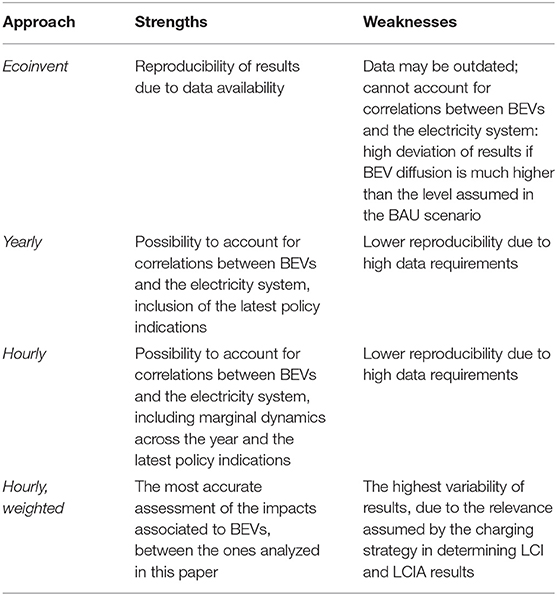
Table 7. Summary of strengths and weaknesses related to different approaches for computing marginal electricity mixes, to be used in LCA for BEV.

Firstly, updating the ecoinvent dataset with the latest policy indications strongly influences the results, even if equation 1 is used in both the Yearly and the Ecoinvent approaches. Then, moving from the Ecoinvent to the Hourly, weighted approach increases the accuracy of results, but decreases their reproducibility. Moreover, the high amount of data required increases the variability of results, too. Integrating an ESM within the LCA requires a high number of assumptions, which may be hard to manage depending on the geographical scale and on the chosen model. The higher the geographical scale, the more complete the assessment is, yet the higher is the number of data and assumptions required, too. However, if the geographical scale is smaller, e.g., city or regional level, such complexity may be managed with accurate data and models and the variability of results may be more easily assessed. Our framework can flexibly be coupled with different geographical scales or ESMs: the methodology would not change.

Conclusions

This study aimed at providing an insight on the relevance of non-linearities in LCA results for future BEVs diffusion in Italy, which emerge when LCI correlations between the fleet of vehicles and the electricity grid are accounted for. Marginal electricity supply mixes are thus explicitly modeled in the foreground system, being them dependent on the number of circulating BEVs. This is achieved due to EnergyPLAN ESM, which models both the electricity system and the BEVs fleet. Five different scenarios of 2030 BEVs market penetration are computed, the first being the BAU scenario. Across the remaining four scenarios, the diffusion of BEVs into the Italian passenger car fleet is modeled up to 100% of the total, with four steps of 25% each.

Our contribution is 3-fold. Firstly, three different approaches for building the LCI are summarized, based on indications from the literature and on the possibilities provided by EnergyPLAN. The Yearly approach computes marginal electricity mixes based on differences in yearly electricity production by technology. The Hourly approach exploits the hourly time resolution of EnergyPLAN and computes yearly marginal electricity production by summing up the hourly differences of electricity production by technology. Finally, the Hourly, weighted approach weights hourly marginal mixes on BEVs charge profiles.

Secondly, we found that significant non-linearities may occur across the analyzed scenarios and LCIA categories. We compared LCI and LCIA results with the ecoinvent dataset results, which is employed as reference to quantify the relevance of non-linearities with respect to a conventional LCA approach. The ecoinvent dataset is not computed according to the latest policy indications and does not depend on the amount of circulating BEVs. Our main hypothesis of keeping RES capacity constant across scenarios leads to a progressive increase of natural gas shares at higher numbers of circulating BEVs. Accordingly, we find that Climate change total indicator shows the highest variations across approaches and scenarios, since it is the only selected LCIA indicator which is mainly driven by natural gas consumption. In particular, within our hypotheses, we found differences of unitary impacts, i.e., per kWh of marginal electricity supplied, of about 40% within the BAU scenario, for the Climate change total category, between the Ecoinvent and the Hourly, weighted approaches. Changes of electricity mixes across scenarios cannot be captured by using the constant value of the ecoinvent dataset, which leads to an underestimation of 8.35 Mton CO₂-eq in the 100% BEV scenario, with respect to the Hourly, weighted results. Similarly, linearly scaling the Hourly, weighted results keeping the BAU unitary impact would lead to an underestimation of 12.45 Mton CO₂-eq. The variation of unitary impacts related to the cradle-to-grade BEV LCA is still relevant, with an approximate increase of +33 and +40%, respectively, for the Hourly, weighted and the Yearly approaches, within the Climate change total category, between the BAU and the 100% BEV scenario. Non-linearities still emerge in other LCIA indicators, which progressively decrease at higher BEVs penetration, unlike Climate change total which increases instead. In particular, Minerals and metals and Freshwater eutrophication show a 6.1% decrease of Hourly, weighted unitary impacts, across the two extreme scenarios. Our results for the Climate change total indicator are in the lower part of the ranges defined by literature studies on future BEVs penetration, since we employ a generally clean marginal mix: fossil fuel shares are at most equal to 38.94% in our analyses. The variability of our Climate change total indicator is lower than what is defined by other studies, since we only modified the use phase electricity mix and we did not assess mixes constituted by 100% fossil fuels.

Thirdly, different electricity mixes are found using of the three approaches. In addition to the capabilities of the Yearly approach, the Hourly and Hourly, weighted results can capture the emergence of marginal technologies within specific hours of the year, as happens for natural gas in the BAU scenario. All the three approaches can represent the interaction between the BEVs fleet and the electricity system. However, only the Hourly, weighted curve can fully capture non-linearities associated to the electricity that is actually consumed by BEVs. We acknowledge that employing the Hourly, weighted approach requires a significant amount of data and assumptions. Nonetheless, we recommend this methodology as the most accurate to assess non-linearities in LCA results emerging in response to the increasing amount of circulating BEVs. Indeed, Hourly, weighted is the only approach that correctly accounts for the potential of BEVs to reduce VRES curtailment, especially in low BEVs diffusion scenarios. Moreover, at higher BEVs diffusion, this approach accurately captures the increased fossil fuel power plants response that happens especially in the early morning and in the evening.

The developed framework could be included in holistic assessment of transport systems, such as Bohnes et al. (2017) and Ricardo (2020), in order to provide additional robustness to the policymaking support process. Moreover, our framework could be coupled with different ESMs, such as the one developed in Girardi et al. (2015), or may be evaluated at different geographical scales, such as a city or a region.

Data Availability Statement

The original contributions presented in the study are included in the article/Supplementary Material, further inquiries can be directed to the corresponding author/s.

Author Contributions

DR and SC contributed to the conception of the study. DR designed the methodology, set up the LCA model in brightway2, wrote and edited the manuscript, and curated data visualization. PS set up the energy simulation model in EnergyPLAN, with the supervision of DR. SC contributed in writing the manuscript introduction and providing multiple revisions and editing. DR, SC, PS, GD, and CB contributed to manuscript revision. All authors contributed to the article and approved the submitted version.

Conflict of Interest

The authors declare that the research was conducted in the absence of any commercial or financial relationships that could be construed as a potential conflict of interest.

Acknowledgments

The authors would like to thank the Reviewers for their valuable comments, aimed at improving communication, effectiveness, and the overall quality of the present manuscript.

Supplementary Material

The Supplementary Material for this article can be found online at: https://www.frontiersin.org/articles/10.3389/frsus.2021.631268/full#supplementary-material

References

ACI (2017). Annuario Statistico ACI - Sintesi dei risultati. 1–10. Available online at: http://www.aci.it/fileadmin/documenti/studi_e_ricerche/dati_statistiche/Annuario2017/Capitolo_1_2017.pdf (accessed February 25, 2021).

Amor, M. B., Gaudreault, C., Pineau, P. O., and Samson, R. (2014). Implications of integrating electricity supply dynamics into life cycle assessment: a case study of renewable distributed generation. Renew. Energy 69, 410–419. doi: 10.1016/j.renene.2014.03.063

CrossRef Full Text | Google Scholar

Bahlawan, H., Morini, M., Pinelli, M., Poganietz, W. R., Spina, P. R., and Venturini, M. (2019). Optimization of a hybrid energy plant by integrating the cumulative energy demand. Appl. Energy 253, 1–15. doi: 10.1016/j.apenergy.2019.113484

CrossRef Full Text | Google Scholar

Bauer, C., Hofer, J., Althaus, H. J., Del Duce, A., and Simons, A. (2015). The environmental performance of current and future passenger vehicles: life cycle assessment based on a novel scenario analysis framework. Appl. Energy 157, 871–883. doi: 10.1016/j.apenergy.2015.01.019

CrossRef Full Text | Google Scholar

BloombergNEF (2020). Electric Vehicle Outlook. Available online at: https://about.bnef.com/electric-vehicle-outlook/ (accessed November 11, 2020).

Bohnes, F. A., Gregg, J. S., and Laurent, A. (2017). Environmental impacts of future urban deployment of electric vehicles: assessment framework and case study of copenhagen for 2016-2030. Environ. Sci. Technol. 51, 13995–14005. doi: 10.1021/acs.est.7b01780

PubMed Abstract | CrossRef Full Text | Google Scholar

Brondi, C., Cornago, S., Piloni, D., Brusaferri, A., and Ballarino, A. (2019). “Application of LCA for the short-term management of electricity consumption,” in Life Cycle Assessment of Energy Systems and Sustainable Energy Technologies, eds R. Basosi, M. Cellura, S. Longo, and M. L. Parisi (Cham: Springer Nature Switzerland AG), 45–59. doi: 10.1007/978-3-319-93740-3_4

CrossRef Full Text | Google Scholar

Burchart-Korol, D., Jursova, S., Folega, P., Korol, J., Pustejovska, P., and Blaut, A. (2018). Environmental life cycle assessment of electric vehicles in Poland and the Czech Republic. J. Clean. Prod. 202, 476–487. doi: 10.1016/j.jclepro.2018.08.145

CrossRef Full Text | Google Scholar

Caduff, M., Huijbregts, M. A. J., Althaus, H. J., and Hendriks, A. J. (2011). Power-law relationships for estimating mass, fuel consumption and costs of energy conversion equipments. Environ. Sci. Technol. 45, 751–754. doi: 10.1021/es103095k

PubMed Abstract | CrossRef Full Text | Google Scholar

Capros, P., De Vita, A., Tasios, N., Siskos, P., and Kannavou, M. (2016). EU Reference Scenario 2016 - Energy, Transport and GHG Emissions - Trends to 2050. Luxembourg, 1–220.

Google Scholar

Connolly, D., Hansen, K., Drysdale, D., Lund, H., and Mathiesen, B. V. (2015). Enhanced Heating and Cooling Plans to Quantify the Impact of Increased Energy Efficiency in EU Member States - Translating the Heat Roadmap Europe Methodology to Member State Level - Work Package 2 Country Report, 1–12. Available online at: https://heatroadmap.eu/wp-content/uploads/2018/11/STRATEGO-WP2-Country-Report-Italy.pdf (accessed February 25, 2021).

Cornago, S., Vitali, A., Brondi, C., and Low, J. S. C. (2020). Electricity technological mix forecasting for life cycle assessment aware scheduling. Procedia CIRP 90, 268–273. doi: 10.1016/j.procir.2020.01.099

CrossRef Full Text | Google Scholar

Cox, B., Bauer, C., Mendoza Beltran, A., van Vuuren, D. P., and Mutel, C. L. (2020). Life cycle environmental and cost comparison of current and future passenger cars under different energy scenarios. Appl. Energy 269, 1–13. doi: 10.1016/j.apenergy.2020.115021

CrossRef Full Text | Google Scholar

Cox, B., Mutel, C. L., Bauer, C., Mendoza Beltran, A., and Van Vuuren, D. P. (2018). Uncertain environmental footprint of current and future battery electric vehicles. Environ. Sci. Technol. 52, 4989–4995. doi: 10.1021/acs.est.8b00261

PubMed Abstract | CrossRef Full Text | Google Scholar

Dandres, T., Vandromme, N., Obrekht, G., Wong, A., Nguyen, K. K., Lemieux, Y., et al. (2017). Consequences of future data center deployment in canada on electricity generation and environmental impacts: a 2015–2030 prospective study. J. Ind. Ecol. 21, 1312–1322. doi: 10.1111/jiec.12515

CrossRef Full Text | Google Scholar

Das, H. S., Rahman, M. M., Li, S., and Tan, C. W. (2020). Electric vehicles standards, charging infrastructure, and impact on grid integration: a technological review. Renew. Sustain. Energy Rev. 120, 1–27. doi: 10.1016/j.rser.2019.109618

CrossRef Full Text | Google Scholar

Doucette, R. T., and McCulloch, M. D. (2011). Modeling the CO2 emissions from battery electric vehicles given the power generation mixes of different countries. Energy Policy 39, 803–811. doi: 10.1016/j.enpol,.2010.10.054

CrossRef Full Text | Google Scholar

EC-JRC (2010). International Reference Life Cycle Data System (ILCD) Handbook - General guide for Life Cycle Assessment - Detailed Guidance. Luxembourg, 1–417.

Ekvall, T., Assefa, G., Björklund, A., Eriksson, O., and Finnveden, G. (2007). What life-cycle assessment does and does not do in assessments of waste management. Waste Manag. 27, 989–996. doi: 10.1016/j.wasman.2007.02.015

PubMed Abstract | CrossRef Full Text | Google Scholar

Enel European House Ambrosetti (2017). E-MOBILITY Revolution. Gli impatti sulle filiere industriali e sul sistema-Paese: quale Agenda per l'Italia. 1–166. Available online at: https://www.ambrosetti.eu/wp-content/uploads/ENEL_e-Mobility-Revolution_Ricerca-2017_ITA.pdf (accessed February 25, 2021).

Energy and Strategy Group (2018). E-Mobility Report 2018. Milano: Energy and Strategy Group, 1–266.

Google Scholar

Eurostat (2019). Combined Heat and Power (CHP) Data 2005-2018. Available online at: http://ec.europa.eu/eurostat/web/energy/data (accessed November 8, 2020).

Gestore Mercati Energetici (2020). Italian Electricity Market zones. Available online at: https://www.mercatoelettrico.org/En/Mercati/MercatoElettrico/Zone.aspx (accessed November 8, 2020).

Girardi, P., Gargiulo, A., and Brambilla, P. C. (2015). A comparative LCA of an electric vehicle and an internal combustion engine vehicle using the appropriate power mix: the Italian case study. Int. J. Life Cycle Assess. 20, 1127–1142. doi: 10.1007/s11367-015-0903-x

CrossRef Full Text | Google Scholar

Graff Zivin, J. S., Kotchen, M. J., and Mansur, E. T. (2014). Spatial and temporal heterogeneity of marginal emissions: Implications for electric cars and other electricity-shifting policies. J. Econ. Behav. Organ. 107, 248–268. doi: 10.1016/j.jebo.2014.03.010

CrossRef Full Text | Google Scholar

GSE (2018). Rapporto Statistico: Energia da fonti rinnovabili in Italia - Anno 2016. 1–196. Available online at: https://www.gse.it/documenti_site/DocumentiGSE/Rapportistatistici/RapportostatisticoGSE-2016.pdf (accessed February 25, 2021).

Heijungs, R. (2020). Is mainstream LCA linear? Int. J. Life Cycle Assess. 25, 1872–1882. doi: 10.1007/s11367-020-01810-z

CrossRef Full Text | Google Scholar

Heijungs, R., and Suh, S. (2002). “The computational structure of life cycle assessment,” in Eco-efficiency in Industry and Science, Vol. 11 (Dordrecht: Kluwer Academic Publishers), 1–280. doi: 10.1007/978-94-015-9900-9

CrossRef Full Text | Google Scholar

Huo, H., Cai, H., Zhang, Q., Liu, F., and He, K. (2015). Life-cycle assessment of greenhouse gas and air emissions of electric vehicles: a comparison between China and the U.S. Atmos. Environ. 108, 107–116. doi: 10.1016/j.atmosenv.2015.02.073

CrossRef Full Text | Google Scholar

IEA (2019). Offshore Wind Outlook. Available online at: https://www.iea.org/reports/offshore-wind-outlook-2019 (accessed November 11, 2020).

IEA (2020). Global EV Outlook. Available online at: https://www.iea.org/reports/global-ev-outlook-2020 (accessed November 11, 2020).

IPCC (2013). “Climate change 2013: the physical science basis,” in Contribution of Working Group I to the Fifth Assessment Report of the Intergovernmental Panel on Climate Change (Cambridge, UK: IPCC), 1–1535.

Google Scholar

Jian, L., Zheng, Y., and Shao, Z. (2017). High efficient valley-filling strategy for centralized coordinated charging of large-scale electric vehicles. Appl. Energy 186, 46–55. doi: 10.1016/j.apenergy.2016.10.117

CrossRef Full Text | Google Scholar

Laurent, A., and Espinosa, N. (2015). Environmental impacts of electricity generation at global, regional and national scales in 1980-2011: what can we learn for future energy planning? Energy Environ. Sci. 8, 689–701. doi: 10.1039/C4EE03832K

CrossRef Full Text | Google Scholar

Lund, H. (2014). Renewable Energy Systems: A Smart Energy Systems Approach to the Choice and Modeling of 100% Renewable Solution. (Oxford: Elsevier), 1–384.

Google Scholar

Lund, H., Mathiesen, B. V., Christensen, P., and Schmidt, J. H. (2010). Energy system analysis of marginal electricity supply in consequential LCA. Int. J. Life Cycle Assess. 15, 260–271. doi: 10.1007/s11367-010-0164-7

CrossRef Full Text | Google Scholar

Lund, H., and Thellufsen, J. Z. (2020). EnergyPLAN - Advanced Energy Systems Analysis Computer Model (Version 15.1). Aalborg, 1–189.

Marmiroli, B. (2020). Sustainability Assessment of Electric Mobility. Milano, 1–209.

Google Scholar

Marmiroli, B., Messagie, M., Dotelli, G., and Van Mierlo, J. (2018). Electricity generation in LCA of electric vehicles: a review. Appl. Sci. 8:1384. doi: 10.3390/app8081384

CrossRef Full Text | Google Scholar

Mathiesen, B. V., Münster, M., and Fruergaard, T. (2009). Uncertainties related to the identification of the marginal energy technology in consequential life cycle assessments. J. Clean. Prod. 17, 1331–1338. doi: 10.1016/j.jclepro.2009.04.009

CrossRef Full Text | Google Scholar

Mclaren, J., Parkinson, S., and Jackson, T. (2000). Modelling material cascades-frameworks for the environmental assessment of recycling systems. Resour. Conserv. Recycl. 31, 83–104. doi: 10.1016/S0921-3449(00)00073-2

CrossRef Full Text | Google Scholar

Mehrjerdi, H., and Rakhshani, E. (2019). Vehicle-to-grid technology for cost reduction and uncertainty management integrated with solar power. J. Clean. Prod. 229, 463–469. doi: 10.1016/j.jclepro.2019.05.023

CrossRef Full Text | Google Scholar

Messagie, M., Mertens, J., Oliveira, L., Rangaraju, S., Sanfelix, J., Coosemans, T., et al. (2014). The hourly life cycle carbon footprint of electricity generation in Belgium, bringing a temporal resolution in life cycle assessment. Appl. Energy 134, 469–476. doi: 10.1016/j.apenergy.2014.08.071

CrossRef Full Text | Google Scholar

MiSE, MATTM, and MIT. (2018). Proposta di Piano Nazionale Integrato per l'Energia e il Clima (PNIEC). 1–237. Available online at: https://www.mise.gov.it/images/stories/documenti/PNIEC_finale_17012020.pdf (accessed February 25, 2021).

Google Scholar

MiSE and MATTM. (2017). Strategia Energetica Nazionale (SEN), 1–308. Available online at: https://www.mise.gov.it/images/stories/documenti/Testo-integrale-SEN-2017.pdf (accessed February 25, 2021).

Google Scholar

Mutel, C. (2017). Brightway: an open source framework for Life Cycle Assessment. J. Open Source Sci. 2, 1–2. doi: 10.21105/joss.00236

CrossRef Full Text

Nordelöf, A., Messagie, M., Tillman, A. M., Ljunggren Söderman, M., and Van Mierlo, J. (2014). Environmental impacts of hybrid, plug-in hybrid, and battery electric vehicles—what can we learn from life cycle assessment? Int. J. Life Cycle Assess. 19, 1866–1890. doi: 10.1007/s11367-014-0788-0

CrossRef Full Text | Google Scholar

Rangaraju, S., De Vroey, L., Messagie, M., Mertens, J., and Van Mierlo, J. (2015). Impacts of electricity mix, charging profile, and driving behavior on the emissions performance of battery electric vehicles: a Belgian case study. Appl. Energy 148, 496–505. doi: 10.1016/j.apenergy.2015.01.121

CrossRef Full Text | Google Scholar

Ricardo (2020). Determining the Environmental Impacts of Conventional and Alternatively Fuelled Vehicles Through LCA. 1–456. Available online at: https://op.europa.eu/en/publication-detail/-/publication/1f494180-bc0e-11ea-811c-01aa75ed71a1 (accessed February 25, 2021).

Richardson, D. B. (2013). Electric vehicles and the electric grid: a review of modeling approaches, impacts, and renewable energy integration. Renew. Sustain. Energy Rev. 19, 247–254. doi: 10.1016/j.rser.2012.11.042

CrossRef Full Text | Google Scholar

Roux, C., Schalbart, P., and Peuportier, B. (2017). Development of an electricity system model allowing dynamic and marginal approaches in LCA—tested in the French context of space heating in buildings. Int. J. Life Cycle Assess. 22, 1177–1190. doi: 10.1007/s11367-016-1229-z

CrossRef Full Text | Google Scholar

RSE (2017). Decarbonizzazione dell' economia italiana: scenari di sviluppo del sistema energetico nazionale. 2017, 1–164. Available online at: https://www.minambiente.it/sites/default/files/archivio/allegati/rse_decarbonizzazione_web.pdf (accessed February 25, 2021).

Google Scholar

Sala, S., Pant, R., Hauschild, M., and Pennington, D. (2012). Research needs and challenges from science to decision support. Lesson learnt from the development of the international reference life cycle data system (ILCD) recommendations for life cycle impact assessment. Sustainability 4, 1412–1425. doi: 10.3390/su4071412

CrossRef Full Text | Google Scholar

Sala, S., Reale, F., Cristobal-Garcia, J., Marelli, L., and Pant, R. (2016). Life Cycle Assessment for the Impact Assessment of Policies. Luxembourg: European Commission, 1–53.

PubMed Abstract | Google Scholar

Siret, C., Tytgat, J., Ebert, T., Mistry, M., Thirlaway, C., Schutz, B., et al. (2018). Product Environmental Footprint Category Rules for High Specific Energy Rechargeable Batteries for Mobile Applications. 1–98. Available online at: https://ec.europa.eu/environment/eussd/smgp/pdf/PEFCR_Batteries.pdf (accessed February 25, 2021).

Terna (2016). Impianti di generazione. 31–71. Available online at: https://download.terna.it/terna/0000/0964/25.PDF (accessed February 25, 2021).

Terna (2018). Monthly Report on the Electricity System - January. 1–31. Available online at: https://download.terna.it/terna/0000/1041/52.PDF (accessed February 25, 2021).

Terna (2020). Transparency Report. Available online at: https://www.terna.it/it/sistema-elettrico/transparency-report (accessed August 31, 2020).

Google Scholar

Vandepaer, L., Treyer, K., Mutel, C., Bauer, C., and Amor, B. (2019). The integration of long-term marginal electricity supply mixes in the ecoinvent consequential database version 3.4 and examination of modeling choices. Int. J. Life Cycle Assess. 24, 1409–1428. doi: 10.1007/s11367-018-1571-4

CrossRef Full Text | Google Scholar

Wernet, G., Bauer, C., Steubing, B., Reinhard, J., Moreno-Ruiz, E., and Weidema, B. (2016). The ecoinvent database version 3 (part I): overview and methodology. Int. J. Life Cycle Assess. 21, 1218–1230. doi: 10.1007/s11367-016-1087-8

CrossRef Full Text | Google Scholar

Yang, Y. (2017). Rethinking system boundary in LCA—reply to “Lifting the fog on the characteristics and limitations of hybrid LCA” by Thomas Gibon and Thomas Schaubroeck (2017). Int. J. Life Cycle Assess. 22, 1009–1011. doi: 10.1007/s11367-017-1295-x

CrossRef Full Text | Google Scholar