Exploring ESG volatility spillovers: evidence from global equity markets

This paper investigates the volatility spillover between sustainable stocks proxied by six ESG equity indices of different geographical areas using daily returns from 2014 to 2022. We apply the Granger causality test to understand return relationships, the impulse response analysis, and the Diebold-Yilmaz spillover index. Results show that ESG equity indices are interrelated. Companies with a good ESG profile in emerging markets and clean technology are more subject to external shocks and thus more vulnerable. Understanding how risk spillover evolve and distribute across the global market in the ESG environment is key to investors and policymakers willing to foster sustainable growth.

1 Introduction

Over the last decades, investors' awareness of sustainability and ESG investing has grown: investors have started questioning the traditional “shareholder value” approach to evaluating corporate value. Additionally, policymakers have designed several policies to promote sustainable development and ESG disclosure, aiming to hold companies accountable for their impact on the planet and societies (Townsend, 2020; Ballestero et al., 2012).

Investors employ various investment strategies to incorporate sustainable equities into their portfolios. Negative screening excludes non-sustainable companies or sectors from asset allocation, while positive screening (or “best-in-class”) targets only companies or industries considered “sustainable” or “socially responsible.”

Retail investors remain skeptical about sustainable or ESG funds (Al-Hiyari and Kolsi, 2021; Petelczyc, 2022), whereas most institutional investors integrate ESG strategies into their portfolios.¹ In the asset management industry, socially responsible or ESG funds have grown considerably in recent years (Carlsson Hauff and Nilsson, 2023), supported by the adoption of a harmonized definition of “sustainability” (UNCTAD, 2021; Global Sustainable Investment Alliance, 2021) and the development of specific ESG indices. To reach the net zero, GSIA estimated in 2023 a size of sustainable finance of around $30.3 trillion [Global Sustainable Investment Alliance (GSIA), 2023], while other estimates are even higher (e.g., 43 trillion by Deloitte, 2024). According to Morningstar (2024) estimates, the total asset under management by institutional investors in 2023 reached around 3,000 billions and the vast majority of fund managers report ESG investing is a priority (IIA, 2022). ESG criteria have been gradually included not only in equities portfolio, but also fixed income (76% of fund managers included ESG in fixed income in 2022 compared to 42% in 2021) (IIA, 2022).

ESG investors focus on specific ESG benchmarks that synthetically track the stock returns of listed companies with strong ESG performance. Many of these benchmarks emphasize firms' environmental performance and their impact on climate change (Global Sustainable Investment Alliance, 2021; Agosto et al., 2023).

The literature compares ESG and traditional investment strategies and examines the effects of ESG inclusion on portfolio performance (Ur Rehman et al., 2016; Giese et al., 2019; Cerqueti et al., 2021). However, little is still known about the risks embedded in ESG equity investments (Karoui and Nguyen, 2022; Sabbaghi, 2023), and particularly about volatility spillovers between different ESG indices of different geographical areas (Sharma et al., 2022) or different industry markets. Only a limited number of studies explicitly examine ESG spillovers, leaving significant scope for further research and leaving several questions yet to be addressed.

This paper addresses this gap by exploring the relationships among six different ESG equity indices using three distinct methods: the Granger causality test, impulse response analysis, and the Diebold-Yilmaz volatility spillover index (Diebold and Yilmaz, 2009, 2012). We test the relationships existing between the ESG indices and also include a traditional index (S&P Oil) to capture potential spillovers not only between different geographical or industry markets, but also between the traditional market and sustainable ones.

ESG equity indices are found to be significantly interrelated. ESG-compliant companies located in emerging markets and clean technologies appear more susceptible to external shocks and are therefore more vulnerable. This represents a critical concern for both investors and policymakers. These markets play a pivotal role in enabling a smooth transition to a more sustainable economic system. Understanding how risks evolve and spread across the global ESG market is essential for investors aiming to finance sustainable businesses and for policymakers seeking to promote greener growth.

The paper is structured as follows: Section 2 presents a literature review focused on key methodological studies on ESG and spillovers; Section 3 outlines the data and methodology; Section 4 discusses the results. The final section concludes.

2 Volatility spillovers

The literature on volatility spillovers is wide and increasing in volume after the contributions of Diebold and Yilmaz (2009, 2012, 2014), but the literature contributions dedicated to ESG volatility spillover are relatively less and still expanding.

Among the studies published to date, many investigate the Environmental dimension in the ESG, namely spillovers between the traditional markets (mainly proxied by the oil index) and green energy sectors through variance decompositions from a vector auto-regression approximating model by Diebold and Yilmaz (2009, 2012, 2014) and their extensions.

In this paragraph, we review and summarize the most relevant studies on ESG volatility spillovers, adopting a wide definition of ESG, hence including also studies on clean energy and sustainable indexes.

Among the most relevant papers, Henriques and Sadorsky (2018) apply Vector Autoregression (VAR) to study the relationship between oil price changes, clean energy stock prices, and technology stock prices. They find the impact of oil prices on alternative energy stock prices is smaller than the impact from technology stock prices. Kumar et al. (2012) applied a VAR model for studying the relationship among clean energy stock prices, oil prices and carbon prices and they concluded that oil prices could affect the stock prices of clean energy firms, while the correlation only exists in the economic recession period. These findings were further extended by Sadorsky (2012), who modeled conditional correlations and examined volatility spillovers between oil prices and the stock prices of clean energy and technology companies. Their results, based on four multivariate GARCH models (BEKK, diagonal, constant conditional correlation, and dynamic conditional correlation), revealed that clean energy stock prices exhibit stronger correlations with technology stock prices than with oil prices. Supporting this line of inquiry, other studies—such as Dutta and Hasib Noor (2017), Reboredo et al. (2017), Reboredo and Ugolini (2018), Reboredo et al. (2019)—demonstrated that incorporating crude oil price fluctuations can enhance the accuracy of volatility forecasts for clean energy stocks. Part of the literature also included bonds in their evaluation: for instance, Reboredo and Ugolini (2020) uses a green bond index with MSCI World and Energy indices and find that price spillovers between green bonds and the stock market are relatively weak or insignificant. Elsayed et al. (2020) explored the temporal patterns of volatility transmission between energy markets and major global financial markets. They found that both the World Stock Index and the World Energy Index act as primary transmitters of volatility to the clean energy sector, with the influence of energy markets on global financial systems becoming especially pronounced during and after financial crises.

Expanding on the notion of directional spillovers, Urom et al. (2022) employed a time-varying parameter VAR model with stochastic volatility to analyze how uncertainty in oil prices affects clean energy sectors. Using wavelet and Cross-Quantilogram techniques, they found that both the direction and magnitude of clean energy sector responses vary significantly across different sectors. These variations are also influenced by prevailing market conditions and investment horizons. Importantly, their results show that spillovers from oil price uncertainty are more substantial over intermediate and long-term horizons. Umar et al. (2022) applies wavelet analysis to explore the relationship between ESG index volatility and financial panic across both time and frequency domains.

Within the frequency connectedness framework proposed by Baruńık and Křehĺık (2018), Ferrer et al. (2018) analyzed the co-movement of returns and volatilities across various time frequencies. Their study focused on stock prices of U.S. alternative energy companies, crude oil prices, and several major financial variables—including high-tech and conventional energy stocks, U.S. 10-year Treasury bond yields, the U.S. default spread, and the volatilities of U.S. equity and Treasury markets. Their results suggest that most of the return and volatility linkages occur over short-term horizons, and that crude oil prices are not the dominant factor driving the performance of renewable energy companies.

By employing a quantile vector autoregression framework, Khalfaoui et al. (2022) have investigated time-frequency transmission and connectedness among green indices. Evidence from empirical results has shown high spillover and volatility effects among the indices and a strong connectedness between climate change indices at extreme lower and extreme upper quantiles.

Taking from the methodological perspectives above cited, recently, a strand of literature has focused on studying volatility spillover between ESG indices in the frequency connectedness framework.

Nevertheless, to the best of our knowledge, only a few studies explicitly model ESG risk spillovers and this leaves room for further investigations and leaves some research questions unanswered. Gao et al. (2022) investigated the risk spillover level and risk contagion mechanism of international ESG stock markets in different frequency domains, showing that the entire system presents a small-world structure, and the internal regions display different risk spillover characteristics.

Cagli et al. (2022) examined the dynamic connection and volatility spillovers between commodities and sustainable firms, highlighting volatility spillovers between ESG indices covering the USA, developed and emerging markets, and commodity indices including energy, industrial metals, and precious metals. Their findings indicate that all ESG indices are net volatility transmitters and that all commodity indices other than crude oil and copper are net volatility receivers. ESG volatility spillovers for the BRICS market are investigated by Sahoo and Kumar (2022), who find bi-directional causality among the four ESG indices and unidirectional causality from Brazil, South Africa, and India to China. Papathanasiou et al. (2022) analyzed the volatility transmissions between Growth and ESG stocks, showing that the volatility transmissions tend to increase in intensity and magnitude during periods of turmoil.

3 Materials and methods

To analyze risk spillovers in the ESG domain, in this work, we surveyed the literature dealing with ESG indexes, especially in the domain of volatility spillover. We found many indices employed by the literaure and we searched all the indices in Refinitiv Eikon database to extract historical prices. Of the 15 ESG stock indexes surveyed, only 5 had sufficient data to be included in the analysis. We retained, hence five ESG/clean energy indexes, all published by established Index providers (e.g., Standard & Poor's or MSCI). Given the importance in the literature attributed to energy indexes, we added the SP_OIL Index to capture traditional energy dynamics.

The selection of these indices is guided by the need to ensure global coverage, sectoral diversity, and alignment with widely recognized ESG standards. Each index reflects unique regional or thematic dimensions of ESG investing, thus supporting a multidimensional analysis of risk transmission within and across sustainability-linked equity markets (Table 1).

Table 1

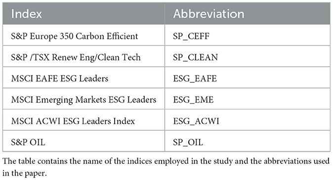
Table 1. Market indices employed in the study.

From a geographical perspective, the MSCI ACWI ESG Leaders index includes large- and mid-cap companies with superior ESG performance across both developed and emerging markets worldwide (ESG_ACWI). The MSCI EAFE ESG Leaders index focuses on developed markets outside North America, specifically Europe, the Asia-Pacific region, and the Far East, providing insight into ESG practices within mature, highly regulated economies (ESG_EAFE). The MSCI Emerging Markets ESG Leaders index targets ESG leaders in developing economies such as China, India, Brazil, and South Africa. It is particularly relevant for understanding ESG dynamics in regions characterized by higher geopolitical and macroeconomic volatility, offering insight into the vulnerability of these markets to both sustainability-related and traditional shocks (ESG_EME).

On the sectoral side, the S&P Europe 350 Carbon Efficient (SP_CEFF) and S&P/TSX Renewable Energy & Clean Technology (SP_CLEAN) indices provide targeted exposure to firms leading in carbon efficiency and clean energy innovation, two strategic pillars of the environmental transition and core elements of climate-aligned investment strategies. These indices allow for the analysis of sector-specific ESG dynamics, particularly in industries that are directly linked to decarbonization efforts and technological transformation.

To establish a comparative baseline with conventional energy markets, the S&P Oil Index is included as a traditional benchmark tracking the performance of fossil fuel companies. This contrast enables the assessment of volatility linkages between ESG-compliant and non-ESG market segments, particularly under conditions of systemic stress or during phases of accelerated energy transition.

We obtainded daily data from Refinitiv Eikon for the most recent period after running the research. After cleaning the dataset, we are left with 2021 observations from 15 September 2014 to 7 June 2022 of five ESG indices with different geographical scope or sectorial specialization and one traditional index (SP_OIL), also to evaluate possible spillovers between sustainable markets and traditional ones as already briefly discussed.

Before studying the volatility spillovers, we first analyze return patterns. We therefore compute the return series, calculated by the logarithmic difference method of R_t = log(P_t)−log(P_t−1). Price dynamics are shown in Figures 1, 2. The graphs show an increasing trend, but all the series experience a strong fall in price in the early 2020, as a probable outcome of the COVID-19 pandemic outbreak and diffusion. After that, the ESG indices show a positive pattern until the early 2022, as rising prices and the Ukrainan conflict, coupled with increasing inflation rates and interest rates might have exerted a negative influence on the performance of ESG leaders (Shahzad et al., 2023). Additionally, SP_OIL shows an increasing trend, overall, probably due to the rising costs of commodities, also fueled by the Ukrainian war (Min, 2022; Škare et al., 2022). The descriptive statistics of the return of ESG indices are presented in Table 2.

Figure 1

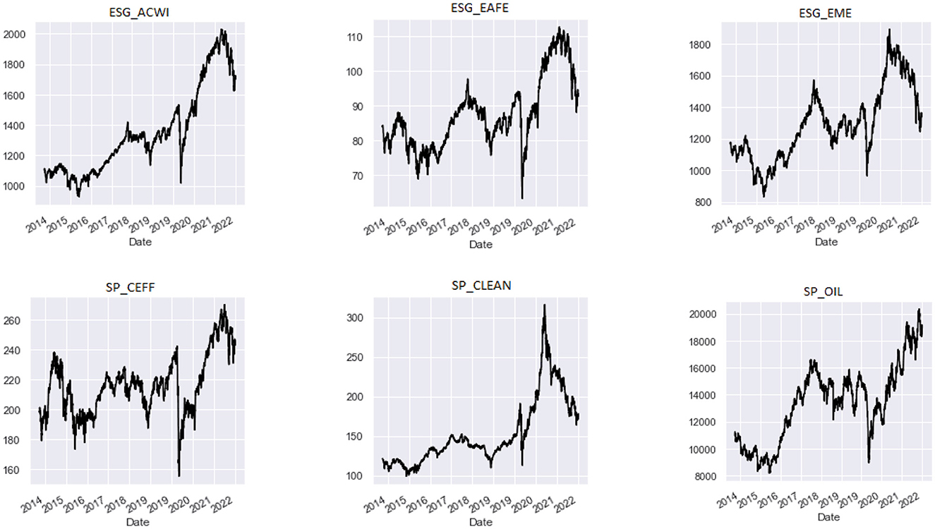
Figure 1. Price dynamic of each index. The figure shows the price behavior of the indices included in the study over the time period 2014–2022.

Figure 2

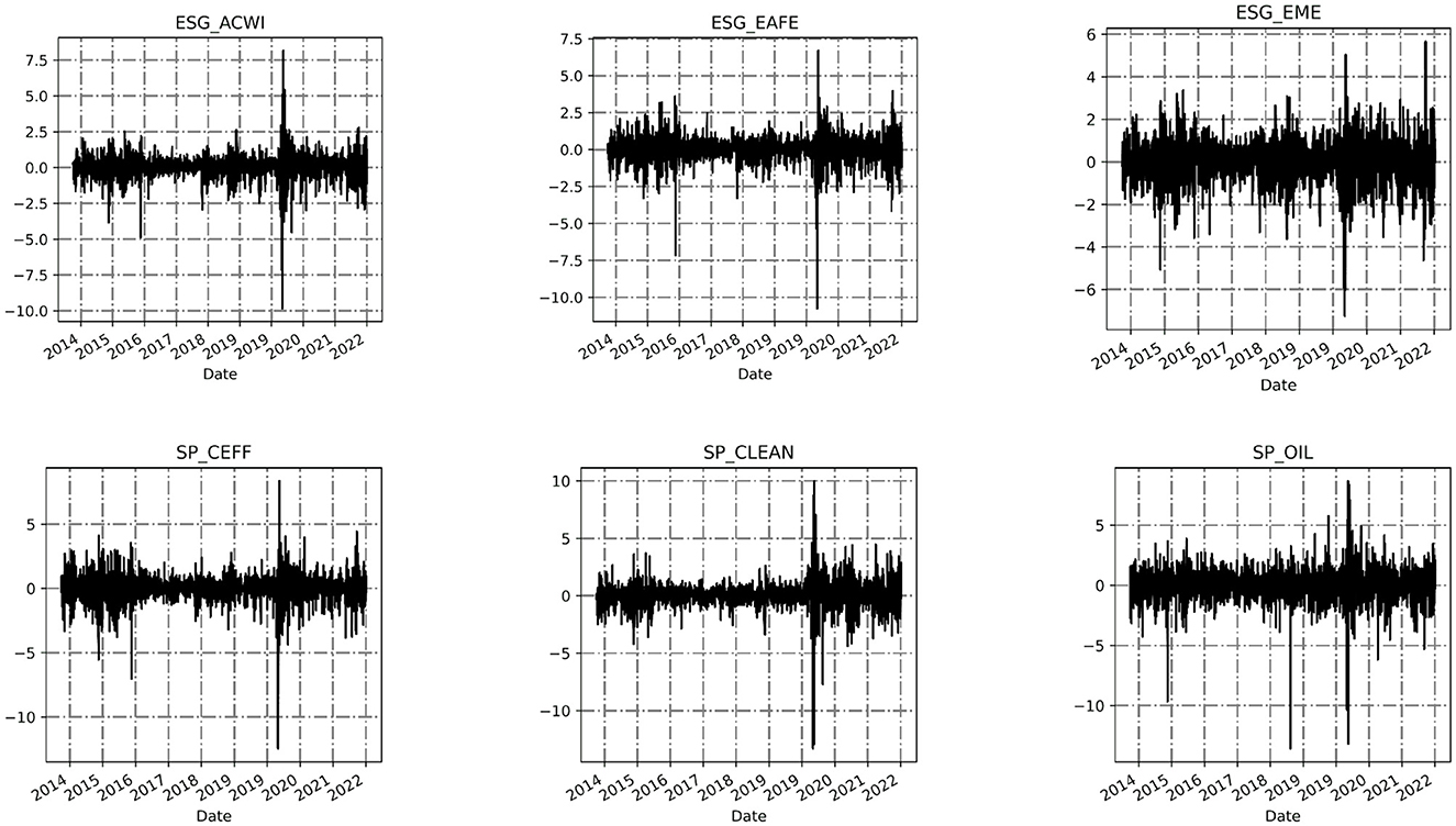
Figure 2. Dynamic trends of each sequence return. The figure shows the return dynamic of the indices included in the study over the time period 2014–2022.

Table 2

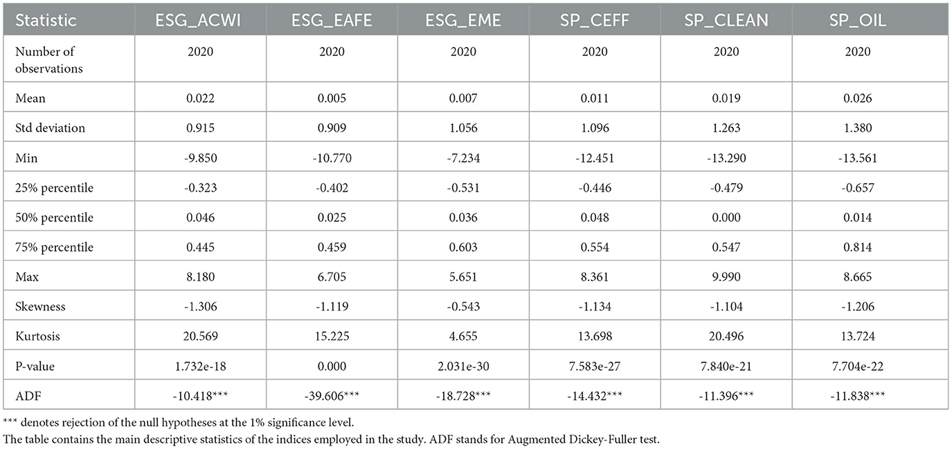
Table 2. Descriptive statistics on indices' returns.

Table 2 reports the descriptive statistics for the daily returns of the selected indices over the sample period, highlighting distinct returns, volatilities, and distributional features across ESG and non-ESG market segments. The empirical results confirm heterogeneous behavior across the indices, justifying their inclusion in the volatility spillover framework. The inclusion of percentiles provides additional insight into dispersion and asymmetry, complementing the analysis of higher-order moments. These distributional properties justify the construction of a spillover framework that accounts for varying tail risks, sectoral dynamics, and regional sensitivities within sustainable and conventional equity markets.

The ESG_ACWI shows a positive mean daily return (0.022) with moderate volatility (standard deviation: 0.915). The interquartile range (IQR), suggests a relatively balanced distribution with limited dispersion around the median. However, the series is left-skewed (-1.306) and leptokurtic (kurtosis: 20.57), indicating exposure to occasional sharp negative movements.

The MSCI EAFE ESG Leaders (ESG_EAFE) presents a lower mean return (0.005) and similar standard deviation (0.909), with an IQR from -0.443 to 0.462. This points to slightly tighter dispersion but continued asymmetry (skewness: -1.119) and fat tails (kurtosis: 15.23), signaling sensitivity to tail risks during market stress.

The MSCI ESG Emerging Markets (ESG_EME) registers a mean return of 0.007 and higher volatility (1.056), with an IQR from -0.553 (25%) to 0.586 (75%), reflecting wider variability. The distribution is less skewed (-0.543) but still leptokurtic (kurtosis: 4.66), confirming its vulnerability to external shocks. The S&P Europe 350 Carbon Efficient (SP_CEFF) has a mean return of 0.011 and standard deviation of 1.096, with percentiles ranging from -0.548 to 0.582. The data reveal substantial dispersion and pronounced asymmetry (skewness: -1.134), suggesting heightened sensitivity to downside shocks, likely linked to policy and commodity price shifts in the European context.

The S&P/TSX Renewable Energy & Clean Technology (SP_CLEAN) shows the most volatile ESG profile (std. dev.: 1.263), with a relatively high mean return (0.019). Its interquartile spread (-0.707 to 0.674) and extreme kurtosis (20.50) point to frequent large swings, particularly on the downside (skewness: -1.104), consistent with the volatility typical of emerging clean energy technologies and regulatory exposure. The S&P Oil Index (SP_OIL) displays the highest overall volatility (1.380) and mean return (0.026), with wide percentiles (25%: -0.738; 75%: 0.761). Its distribution is heavily skewed left (-1.206) and leptokurtic (13.72), highlighting its strong exposure to extreme movements tied to geopolitical instability and commodity price shocks.

As briefly mentioned, the considered timeframe for this study includes the COVID-19 pandemic (2020) and the Russia-Ukraine war (from 2022 onward), making it particularly relevant for analyzing the impact of such exogenous shocks on financial market behavior.

Employing the Pruned Exact Linear Time (PELT) algorithm (Killick et al., 2012), which allows efficient identification of breakpoints in the statistical properties of a time series, we observed changes in both the mean and variance. This method utilizes a cost function based on the Radial Basis Function (RBF) kernel, which is particularly sensitive to joint shifts in location and dispersion. This approach detects points in time where the mean and variance of returns shift significantly. The results show that several assets exhibit distinct breakpoints around the time of the aforementioned crises, underscoring the substantial influence of global economic events on the structure of financial data and the importance of accounting for such shifts in econometric analysis (Figure 3). This evidence paves the way for future research on the effect of such breaks on the structure of volatility spillovers, and it will be taken into consideration when commenting our results.

Figure 3

Figure 3. Dynamic trends and structural breaks in return series over 2014–2022. The figures show significant shifts in the mean and variance of returns across time, as detected by the PELT algorithm.

3.1 Returns and volatilities

In this section, the daily price, squared daily returns (RV) and Realized Semivariance (RS) for the ESG indices are described. Squared daily returns (RV) is a financial metric that measures the actual volatility of an asset's price over a given time period. It is calculated based on the realized or actual returns of the asset, rather than the expected or implied returns. RV is often used to assess the risk associated with an investment and to inform trading decisions. It is commonly used in financial modeling, risk management, and the development of investment strategies. Typically, RV is used as a financial metric allowing to capture the variation in asset prices over a given time period. Quite generally, we can mathematically define the RV as the sum of squared returns over a fixed time interval, T:

$\begin{array}{cc}R{V}_T={\displaystyle \sum _{t=1}^T}{r}_t^2& (1)\end{array}$

where r_t is the return of the asset at time t. RV is often expressed in annualized terms by multiplying it by the number of trading days in a year, D, and taking the square root:

$\begin{array}{cc}R{V}_{T,\text{annualized}}=\sqrt{D·R{V}_T},& (2)\end{array}$

even if, in practice, RV is typically calculated using high-frequency data, such as tick data or intra-day data. One common approach is to use the sum of squared returns over a fixed time interval of Δt, such as 5 min or 1 h:

$\begin{array}{cc}R{V}_{\Delta t}={\displaystyle \sum _{t=1}^{T/\Delta t}}{r}_{t\Delta t}^2& (3)\end{array}$

where r_tΔt is the return of the asset over the time interval Δt starting at time (t−1)Δt. The annualized RV is then computed analogously as we have seen before, namely:

$\begin{array}{cc}R{V}_{\Delta t,\text{annualized}}=\sqrt{D/\Delta t·R{V}_{\Delta t}},& (4)\end{array}$

accordingly, RV is often used as a measure of market risk, as higher volatility implies higher risk and, as a consequence, it has been widely implemented in the calculation of option prices, as the volatility of the underlying asset is a key determinant of option prices.

Andersen and Bollerslev (1998) presented the following definition of the squared daily returns:

$\begin{array}{c}R{V}_t={\displaystyle \sum _1^N}{r}_{t,i}^2,\end{array}$

where RV_t is the RV for day t and r_{t, i} stands for the observed i-returns for day t, and N shows the number of observations of daily returns. Moreover, according to Barndorff-Nielsen et al. (2010), the Realized Semivariance that records variations in daily returns associated with both upward and downward movements is identified. They are defined as follows:

$\begin{array}{c}R{S}_t^{-}={\displaystyle \sum _1^N}{r}_{t,i}^2{I}_{r_{t,i}<0},R{S}_t^{+}={\displaystyle \sum _1^N}{r}_{t,i}^2{I}_{r_{t,i}>0}\end{array}$

Table 3 reports descriptive statistics of squared daily returns for the ESG indices included in the analysis, used as proxies for realized volatility (RV). Figure 4 illustrates the relationship between squared daily returns and price for each ESG index, along with a comparison between the average values of all ESG indices and the average values of their corresponding prices.

Table 3

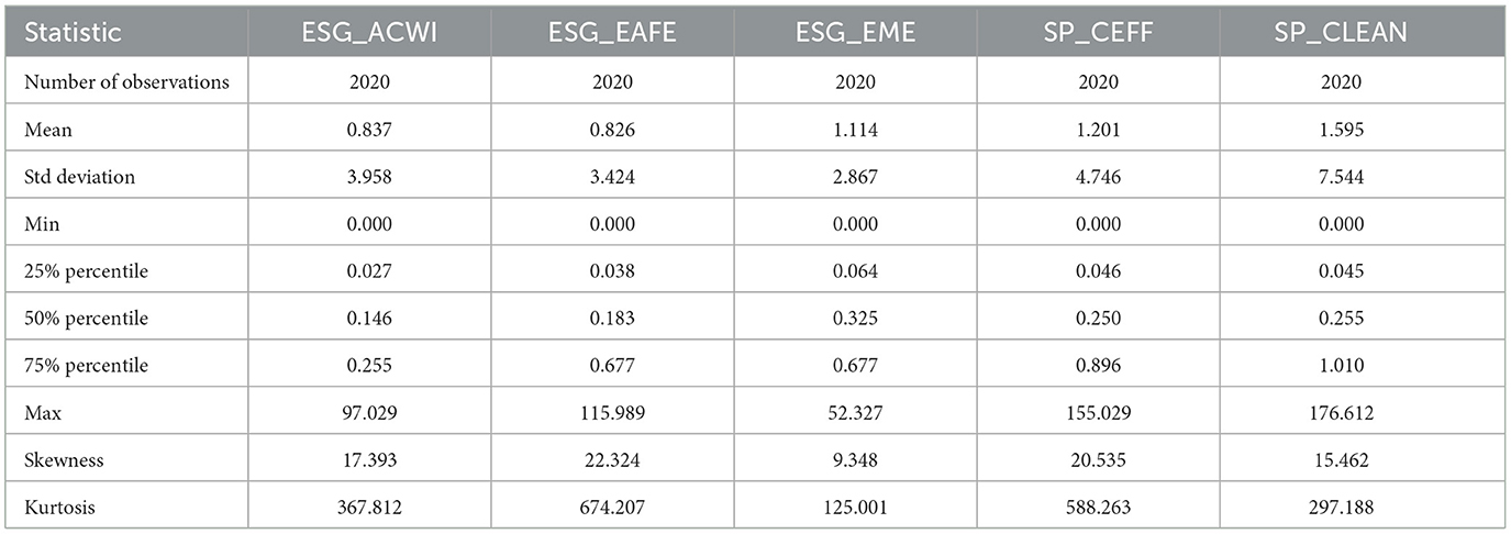
Table 3. Descriptive statistics on indices' squared daily returns.

Figure 4

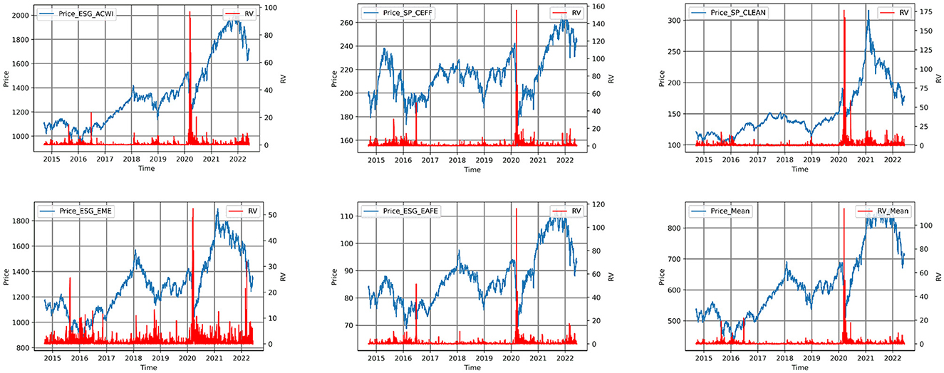
Figure 4. Squared daily returns of each ESG index. The figure shows the squared daily returns the indices included in the study over the time period 2014–2022.

These metrics provide insights into the short-term variability of ESG equity returns and the statistical properties of market risk within each index.

SP_CLEAN stands out with the highest average realized volatility (mean RV = 1.595) and the largest dispersion (standard deviation = 7.544), highlighting its role as a highly volatile thematic index focused on renewable energy and clean technology. The presence of extremely high kurtosis (297.19) and positive skewness (15.46) confirms the occurrence of infrequent but extreme volatility spikes, consistent with its sensitivity to sector-specific shocks and policy uncertainty.

Similarly, SP_CEFF, though less volatile on average (mean RV = 1.201), presents substantial tail risk (kurtosis = 588.26) and extreme skewness (20.54), suggesting that volatility in carbon-efficient European firms is generally low but susceptible to abrupt surges—possibly triggered by macroeconomic or regulatory shocks in the EU energy landscape.

ESG_EME displays a relatively high mean RV (1.114) with the lowest kurtosis (125.00) among the group, indicating more frequent medium-scale volatility, most likely driven by structural instability and heightened exposure to global market turbulence typical of emerging economies. Its skewness (9.35), though elevated, is comparatively lower than that of sectoral indices, implying a more persistent rather than episodic volatility regime.

The global ESG indices, ESG_ACWI and ESG_EAFE, show lower average RV values (0.837 and 0.826 respectively), and relatively moderate skewness and kurtosis, though still indicative of non-normality. These patterns are consistent with their diversified composition and broad market coverage, which tends to smooth out idiosyncratic volatility shocks. Nonetheless, the kurtosis values remain high (367.81 for ESG_ACWI and 674.21 for ESG_EAFE), reinforcing the conclusion that ESG equity volatility, even in diversified portfolios, is characterized by fat-tailed behavior and non-Gaussian dynamics.

In addition to moments, the 25th, 50th (median), and 75th percentiles further enrich the analysis by capturing distribution asymmetry and intra-distribution variability across indices. For instance, SP_CLEAN and SP_CEFF display wide interquartile ranges, highlighting not only higher tail risks but also broader volatility fluctuations in the central part of the distribution. In contrast, the global indices (ESG_ACWI and ESG_EAFE) exhibit narrower percentile spreads, reflecting lower overall variability and reduced frequency of extreme deviations around the median. These percentile-based observations complement the higher-order moments and confirm the asymmetric and regime-dependent nature of volatility dynamics in ESG markets.

These results suggest that ESG indices are heterogeneous not only in terms of return behavior but also in their volatility profiles. The clean energy and carbon-efficient indices are particularly exposed to idiosyncratic, high-magnitude volatility events, whereas globally diversified ESG benchmarks reflect more stable, though still non-linear, risk characteristics. These distinctions are essential for understanding the mechanics of volatility transmission, particularly when assessing asymmetric shock propagation across ESG and non-ESG markets.

In analyzing the dataset, a notable observation can be made from the figure depicting the squared daily returns across different indices. It is evident that during the years 2020 and 2022, the index that exhibited the highest volatility was SP_Clean. Interestingly, when considering the entire duration of our dataset, this index demonstrated relatively lower volatility compared to others. In contrast, the index ESG_EME displayed the considerable volatilities across the entire time range from September 2014 to June 7, 2022. The findings show that while SP_CLEAN experienced a sharp increase in volatility during the specific period of 2020–2022, it generally displayed lower volatility compared to other indices over the entire dataset time-frame. On the other hand, ESG_EME consistently exhibited higher volatility throughout the entire dataset period and ranked second in terms of price volatility. At the end, as we can see in the figure, in average, squared daily returns of ESG indices' price in the considered time period in our dataset is low volatile. As depicted in the figure, we observe that squared daily returns of the average of the ESG index returns within the analyzed time period is relatively low, indicating stability, and we just have a sharp increase in the beginning of 2020.

Furthermore, in Tables 4, 5, we also state the statistical descriptors of squared positive daily returns variance (RV⁺) and squared negative daily returns variance (RV⁻) for the ESG indices in our dataset, respectively.

Table 4

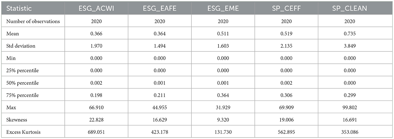
Table 4. Descriptive statistics on indices' squared positive daily returns variance (RV⁺).

Table 5

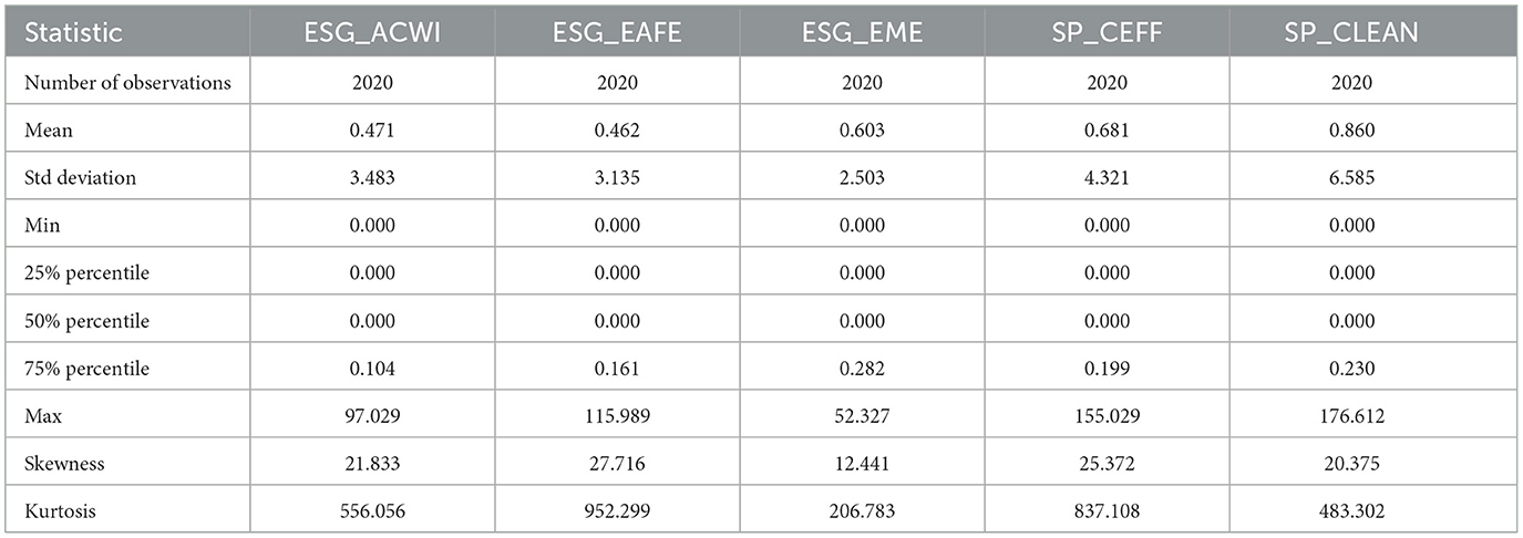
Table 5. Descriptive statistics on indices' squared negative daily returns variance (RV⁻).

Table 4 presents descriptive statistics for the positive realized semivariance (RV⁺) across the five ESG indices, which is employed as a proxy for volatility associated with positive return movements.

Among the indices, SP_CLEAN exhibits the highest mean RV⁺ (0.735) and the greatest dispersion (standard deviation = 3.849), confirming its profile as a highly volatile thematic index. SP_CEFF is the second-highest index in terms of mean RV⁺, which stands at 0.519, and exhibits significant tail risk, as evidenced by its extreme skewness (19.01) and kurtosis (562.90). The percentiles (25% = 0.003; median = 0.013; 75% = 0.214) indicate that, although spikes in positive volatility are relatively rare, they tend to be concentrated and are often associated with carbon pricing shocks within the European market.

ESG_EME index shows a mean RV⁺ of 0.511 and a lower standard deviation (1.603), which indicates moderate but more persistent upside volatility. Conversely ESG_ACWI and ESG_EAFE exhibit lower average RV⁺ values (0.366 and 0.364, respectively), along with narrow interquartile ranges (ESG_ACWI: 0.002-0.093; ESG_EAFE: 0.001-0.108) and low medians (0.006 and 0.003). The high kurtosis values (689.05 for ESG_ACWI; 423.18 for ESG_EAFE) confirm the potential for rare but extreme positive return movements.

The different patterns of RV⁺ over the time considered could serve as a starting point for evaluating the dynamics of realized semivariance over breaks or different regimes.

Table 5 provides some insights into downside risk through RV⁻, highlighting that, across all indices considered, RV⁻ values are consistently higher than RV⁺ values, both in terms of mean and maximum. This asymmetry confirms that the negative component of volatility is not only more frequent but also more intense in ESG equity markets. These findings strengthen the case for adopting semivariance-based metrics to model volatility transmission and capture the inherently asymmetric nature of risk, especially during periods of financial stress or systemic realignments.

SP_CLEAN once again emerges as the index with the highest downside risk (mean RV⁻ = 0.860), coupled with highly pronounced tail behavior (maximum RV⁻ = 176.61; kurtosis = 483.30). SP_CEFF also exhibits severe downside tail risk, with the highest kurtosis overall (837.11) and a substantial mean RV⁻ (0.681), indicating that carbon-efficient portfolios are not immune to intense downward pressure. ESG_EME displays a relatively more balanced risk profile, with moderate downside volatility (mean RV⁻ = 0.603), although its distribution still reveals a degree of asymmetry. Finally, ESG_ACWI and ESG_EAFE, while showing lower average RV⁻ values, maintain very high kurtosis levels, exceeding 550 and 950, respectively.

As observed in Figures 5, 6, it is evident that the highest (RV⁺) was less than the highest (RV⁻) for all ESG indices. Notably, the ESG_EME index exhibits the highest magnitude of both negative and positive semivariance, making it the most volatile index in terms of semivariance within the specified time frame of our dataset. Also, for SP_CLEAN we observe that the after 2020 its positive semivariance was more volatile than before this year. In the average point of view for all indices in our dataset RV⁻ mostly was near zero except in the beginning of 2020 when we have the most RV⁻. Also it seems that in average the RV⁺ is always (except between 2020 and 2021) more than RV⁻.

Figure 5

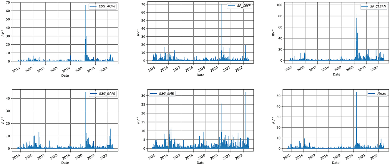
Figure 5. Squared positive daily returns variance (RV⁺) of each ESG index. The figure shows the squared positive daily returns variance of the indices included in the study over the time period 2014–2022.

Figure 6

Figure 6. Squared negative daily returns variance (RV⁻) of each ESG index. The figure shows the squared negative daily returns variance of the indices included in the study over the time period 2014–2022.

3.2 Granger causality

In the literature, a high number of studies highlight the significance of Granger causality tests in explaining the connectedness between variables (e.g., Granger, 1969; Asafu-Adjaye, 2000; Barrett et al., 2010; Bollen et al., 2011). In particular, let us recall that Granger causality is a statistical concept used to determine whether one time series is useful in forecasting another time series. Since its introduction, Granger causality has been widely used in time series analysis. For the sake of completeness let us recall its functioning. Let X(t) and Y(t) be two time series that are observed at discrete time points t = 1, 2, …, T, then the Granger causality test involves fitting two regression models:

$\begin{array}{l}Y(t)=\alpha +{\beta }_{1}Y(t-1)+{\beta }_{2}Y(t-2)+\cdots +{\beta }_{p}Y(t-p)+ϵ(t)\\ Y(t)=\alpha +{\beta }_{1}Y(t-1)+{\beta }_{2}Y(t-2)+\cdots +{\beta }_{p}Y(t-p)\\ +{\gamma }_{1}X(t-1)+{\gamma }_{2}X(t-2)+\cdots +{\gamma }_{q}X(t-q)+ϵ(t)\end{array}$

where p and q are the number of lags in the models, ϵ(t) is the error term for the first model, and ϵ(t) and η(t) are the error terms for the second model. The associated null hypothesis is that X does not Granger-cause Y, which means that the addition of lagged values of X to the second regression model does not improve the forecast of Y beyond what is achieved by the lagged values of Y alone. Accordingly, the alternative hypothesis is that X does Granger-cause Y, which means that the addition of lagged values of X to the second model does improve the forecast of Y. The resulting test statistic is based on the difference in the residual sum of squares (RSS) between the two models, i.e.:

$\begin{array}{cc}F=\frac{(\text{RS}{\text{S}}_1-\text{RS}{\text{S}}_2)/q}{\text{RS}{\text{S}}_2/(T-p-q-1)}& (5)\end{array}$

where q is the number of additional lagged values of X in the second model, and T−p−q−1 is the degrees of freedom for the error term in the second model. Hence, under the null hypothesis, the test statistic F follows an F-distribution with q and T−p−q−1 degrees of freedom, and, if the calculated F-value is greater than the critical F-value from the F-distribution at a chosen significance level, then we reject the null hypothesis and conclude that X Granger-causes Y.

3.3 Impulse response analysis

Impulse response analysis is a method used in Vector Autoregressive (VAR) models to analyze the dynamic response of a set of variables to a shock or innovation in one or more of the variables. In other words, it is helpful to understand how the variables in the model react to a sudden and unexpected change in one of the variables. Let us recall that the VAR model is based on considering y_t to be an n-dimensional vector of variables at time t, where n is the number of variables. Taking ε_t to be an n-dimensional vector of error terms at time t, then the VAR(p) model with p lags reads as follows:

$\begin{array}{cc}{y}_t=c+A_1{y}_{t-1}+A_2{y}_{t-2}+\cdots +A_p{y}_{t-p}+{\epsilon }_t& (6)\end{array}$

where c is an n-dimensional vector of constants, A_i is an n×n coefficient matrix for lag i, and εt is a vector of error terms assumed to be independently and identically distributed with mean zero and covariance matrix Σε. Analogously, we can also express the VAR(p) model in matrix form as:

$\begin{array}{cc}{\text{y}}_t=\text{c}+{\displaystyle \sum _{i=1}^p}{\text{A}}_i{\text{y}}_{t-i}+{\epsilon }_t& (7)\end{array}$

where y_t is an n×1 vector of variables, c is an n×1 vector of constants, A_i is an n×n coefficient matrix for lag i, and ε_t is an n×1 vector of error terms. Accordingly, to estimate the parameters of the VAR(p) model, we need to estimate the coefficient matrices Ai and the covariance matrix Σε. This can be done, e.g., using maximum likelihood estimation, which involves maximizing the log-likelihood function:

$\begin{array}{ll}ℒ\left(c,A_1,A_2,\dots ,A_p,{\Sigma }_{\epsilon }\right)=-\frac{T}{2}\log \left|{\Sigma }_{\epsilon }\right|-\frac{1}{2}{\displaystyle \sum _{t=p+1}^T{\epsilon }_t^{\text{'}}}{\Sigma }_{\epsilon }^{-1}{\epsilon }_t& (8)\end{array}$

where T is the number of time periods in the sample, log|Σ_ε| is the logarithm of the determinant of Σ_ε, and ε_t is the vector of error terms at time t. Then the maximum likelihood estimates of the parameters can be obtained numerically using iterative methods such, e.g., the Newton-Raphson algorithm or the gradient descent algorithm, to then use the VAR(p) model to forecast future values of the variables as well as to perform an impulse response analysis to examine the dynamic effects of shocks to the variables. Consequently, in a VAR model, each variable is modeled as a linear combination of its own lagged values and the lagged values of all other variables in the system, and the coefficients in the VAR model capture the contemporaneous and lagged relationships between the variables.

To perform impulse response analysis in a VAR model, we first identify the variables in the model and the order of the VAR model. Then, we introduce a shock or innovation to one of the variables, which is typically modeled as a one-time deviation from the variable's mean. We can then calculate the response of each variable in the system to this shock over time, using the estimated coefficients in the VAR model.

The impulse response function shows the dynamic response of each variable in the system to the shock over a specified time horizon. The response of each variable is typically presented as a graph, with the y-axis representing the percentage change in the variable and the x-axis representing the time period after the shock. The graphs can help us to identify which variables are affected most by the shock, how long it takes for the effects of the shock to dissipate, and whether there are any delayed or persistent effects on the variables.

Impulse response analysis is a widely used method in both econometrics and signal processing, particularly to investigate the dynamic relationship between variables. It involves estimating the response of a dependent variable to a unit impulse in an independent variable, and then tracing out the subsequent time path of the dependent variable. In particular, let us consider a linear regression model with one independent variable and one dependent variable:

$\begin{array}{cc}{y}_t={\beta }_0+{\beta }_1{x}_t+u_t& (9)\end{array}$

where y_t is the dependent variable, x_t is the independent variable, u_t is the error term, and β₀ and β₁ are the intercept and slope coefficients, respectively. Then, we first need to estimate the model using a suitable method, such as ordinary least squares (OLS). Once the model has been estimated, we can then calculate the impulse response function (IRF) for y_t with respect to a unit impulse in x_t. The IRF is given by:

$\begin{array}{cc}IR{F}_k=\frac{\partial y_{t+k}}{\partial x_t}& (10)\end{array}$

where k is the number of time periods after the impulse. To calculate the IRF, we can use the estimated coefficients from the regression model to obtain the predicted values of y_t for each time period after the impulse, e.g., rewriting the regression equation as:

$\begin{array}{cc}{y}_t={\widehat{\beta }}_0+{\widehat{\beta }}_1{x}_t& (11)\end{array}$

where $\widehat{{\beta }_0}$ and $\widehat{{\beta }_1}$ are the OLS estimates of the intercept and slope coefficients, respectively. If we assume that x_t is equal to zero for all time periods except for period zero, where it is equal to one (i.e., a unit impulse), then the predicted values of y_t for each time period after the impulse can be calculated recursively as:

$\begin{array}{l}{\widehat{y}}_{t+1}={\widehat{\beta }}_0+{\widehat{\beta }}_1·0+u_{t+1}\\ {\widehat{y}}_{t+2}={\widehat{\beta }}_0+{\widehat{\beta }}_1·0+u_{t+2}+{\widehat{\beta }}_1·{\widehat{y}}_{t+1}\\ {\widehat{y}}_{t+3}={\widehat{\beta }}_0+{\widehat{\beta }}_1·0+u_{t+3}+{\widehat{\beta }}_1·{\widehat{y}}_{t+2}& (12)\end{array}$

and so on, until we reach the desired number of time periods after the impulse. Finally, we can calculate the IRF for each time period k by taking the partial derivative of ŷ_t+k with respect to x_t:

$\begin{array}{ll}IR{F}_k=\frac{\partial {\widehat{y}}_{t+k}}{\partial x_t}={\widehat{\beta }}_1·\frac{\partial {\widehat{y}}_{t+k}}{\partial {\widehat{y}}_t}& (13)\end{array}$

where the second term is the partial derivative of ŷt+k with respect to ŷt, which can be obtained using the chain rule of calculus. The resulting IRF indicates how y_t responds to a one-time change in x_t over time, hence providing insight into the dynamic relationship between the two variables. The relevance of IRF to have insights about the question “what is the effect of one unit shock in feature X on feature Y?” is further witnessed by the fact that we can control the standard errors and confidence intervals for the IRF itself by using standard methods for linear regression. Indeed, let ${\widehat{\sigma }}^2$ be the estimated variance of the error term, and let ${\widehat{\sigma }}_{{\beta }_1}^2$ be the estimated variance of the slope coefficient $\widehat{{\beta }_1}$. Then the variance of the IRF at time k is given by:

$\begin{array}{cc}Var\left[IR{F}_k\right]={\widehat{\sigma }}_{{\beta }_1}^2\left({\displaystyle \sum _{j=0}^{k-1}}IR{F}_j^2\right)+2{\widehat{\sigma }}^2\left({\displaystyle \sum _{j=0}^{k-1}}IR{F}_j^2\right)& (14)\end{array}$

where the first term is the variance due to estimation uncertainty in $\widehat{{\beta }_1}$, and the second term is the variance due to stochastic error in the model, then we can then use this variance estimate to calculate the standard error of the IRF at time k as:

$\begin{array}{cc}SE\left[IR{F}_k\right]=\sqrt{Var\left[IR{F}_k\right]}& (15)\end{array}$

accordingly deriving a confidence interval for the IRF using the standard normal distribution:

$\begin{array}{cc}IR{F}_k\pm z_{\alpha /2}SE\left[IR{F}_k\right]& (16)\end{array}$

where z_α/2 is the critical value from the standard normal distribution for a given level of significance α. Additionally, it turns out that IRF allows tracing the transmission of a single shock within an otherwise noisy system of equations and, thus, providing fundamental insights into a plethora of economic and financial scenarios.

Indeed impulse response analysis can be used in the risk management area, where it can help to analyze the dynamic relationships between financial market variables, such as stock prices, interest rates, and exchange rates. Besides, it has been employed also in the studies of macroeconomics, environmental economics, international trade and finance, labor economics and health economics (Kassim et al., 2009; Lütkepohl, 2010; Masih et al., 2011; Abdel-Latif and El-Gamal, 2020). In this work, to estimate the impulse responses, we fitted a standard VAR(9) model, where the lag length was selected using the Akaike Information Criterion (AIC). All variables are daily returns and were confirmed to be stationary using ADF tests. The “shock” referred to throughout this paper denotes a one-unit return innovation in one of the ESG indices and not a macroeconomic shock.

3.4 The DY spillover index

The Diebold and Yilmaz (2012) methodology provides a comprehensive framework for measuring spillover risk in financial markets, which can help investors, policymakers, and regulators to better understand and manage systemic risks. They proposed a methodology to measure spillover risks between financial markets, which involves the following steps:

• Estimating the dynamic conditional correlations (DCC) between the returns of different financial assets, using a multivariate GARCH model.

• Computing the forecast error variance decomposition (FEVD) of each asset's return series over a certain horizon, which captures the percentage of the forecast error variance of each asset's return that can be attributed to its own shocks vs. shocks to other assets.

• Using the FEVD matrix to construct a spillover index, which measures the total spillover risk from all other assets to a particular asset. This index is obtained by summing up the FEVD percentages of all other assets that affect the particular asset.

• Normalizing the spillover index to obtain the spillover intensity index, which measures the relative importance of each asset in transmitting spillover risk to other assets.

• Analyzing the spillover intensity index and the spillover network graph to identify the key drivers of spillover risk and the most vulnerable assets in the network.

In this paper, we follow Diebold and Yilmaz (2009, 2012), as it allows broadly defining the system networks. The technique can be given as follows.

Let Y_t be the n-dimensional column vector of volatility $Y_t=\sum _{j=1}^p{\Theta }_j{Y}_{t-1}+{ϵ}_t$ where Θ_t(N×N) is the autoregressive coefficient matrix and ϵ_t is vector of error terms of dimension N×1 which is also iid. First, we apply a vector autoregressive (VAR(p)) model to the set of ESG indices, which can be derived from following equation:

$\begin{array}{cc}{Y}_j={\displaystyle \sum _{j=1}^{\infty }}{A}_j.{ϵ}_{t-1}& (17)\end{array}$

In Equation 17 the coefficient A_j = 0 where for negative value of j and it becomes an identity matrix of order N whenever j = 0, also it obtains from the following recursive form

$\begin{array}{c}{A}_j={\displaystyle \sum _{i=1}^p}{\psi }_i{A}_{j-i}\end{array}$

whenever j>0. Then, utilizing the information available up to time t+H, we predict future outcomes. Finally, for each element, we examine the error variance of the prediction, attributing it to the shocks caused by that particular element in the system at time t. This approach is similar to common econometric methods of variance decomposition. To determine how much impact a particular variable has on the forecast error variance of other variables, we can use the H-step forward Generalized Forecast Error Variance Decomposition (GFEVD) method. The H-step generalized variance decomposition matrix is given as D(H) = [d_ij(H)] and d_ij(H) denotes pairwise directional spillovers from market j to another market i, and it is given by:

$\begin{array}{cc}{d}_{ij}(H)=\frac{{\sigma }_{jj}^{-1}{\displaystyle {\sum }_{h=0}^{H-1}}{(e_i{A}_h\sum e_j)}^2}{{\displaystyle {\sum }_{h=0}^{H-1}}(e_i{A}_h\sum A_h{e}_j)}& (18)\end{array}$

where σ_jj is the standard error sequence of error vector, ∑ is the covariance matrix of error vector and e_i is an N×1 vector, with one as the i^th element and zero otherwise. Now to make A more comparable, we use following equation to standardize the GFEVD matrix:

$\begin{array}{cc}{d}_{i\leftarrow j}=\frac{d_{ij}(H)}{{\displaystyle {\sum }_{j=1}^N}{d}_{ij}(H)}& (19)\end{array}$

Now, the elements within the matrix quantify the directional risk spillover from market j to market i, and all of them satisfy the conditions $\sum _{j=1}^N{d}_{i\leftarrow j}^H=1$ and $\sum _{i,j=1}^N{d}_{i\leftarrow j}^H=N$. Furthermore, we have the following concepts, related to DY spillovers. The directional DY spillover index can be categorized as either spillover “from others” ($d_{i\leftarrow •}^H$) or spillover “to others” ($d_{•\leftarrow i}^H$), and the difference between these two is called “net spillover”. We have:

$\begin{array}{ll}{d}_{i\leftarrow •}^H=100\times {\displaystyle \sum _{i,j=1,i\ne j}^N{d}_{i\leftarrow j}^H}& (20)\end{array}$

and

$\begin{array}{ll}{d}_{•\leftarrow i}^H=100\times {\displaystyle \sum _{i,j=1,i\ne j}^N{d}_{j\leftarrow j}^H}& (21)\end{array}$

Finally we have total spillover index which quantifies the impact of the spillover effect among N markets on the total variance of forecast errors, and it calculates the average of the elements that are not on the main diagonal:

$\begin{array}{ll}{d}^H=100\times \frac{{\displaystyle {\sum }_{i,j=1,i\ne j}^N{d}_{i\leftarrow j}^H}}{N}.& (22)\end{array}$

4 Results

4.1 Granger causality

In the literature, a high number of studies highlight the significance of Granger causality tests in explaining the connectedness between variables. Bearing this in mind, we use the Granger causality test to understand the connection between different returns of ESG indices. The outcomes of the Granger causality test reveal that almost all the time series in our dataset have a Granger-causal effect on each other (indicated by blue two-sided arrows) at a significant level of 5%. Results of Granger causality are reported in Figure 7. The directional arrows indicate the presence of significant causality between the returns of each ESG index. Each arrow shows statically significant Granger causality (from source to edge of arrow) at 5%. Furthermore, the test results demonstrate that the causal connection among four indices is unidirectional, as displayed in Figure 7 using black one-sided arrows.

Figure 7

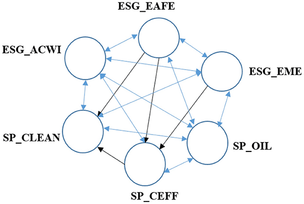
Figure 7. Granger causality test on returns. Arrows indicate a 5% significant Granger causality from the source to the edge of the arrow. Two-sided arrows indicate a 5% significant Granger-causal effect.

Table 6 presents Granger causality test results, highlighting significant directional relationships among ESG indices and the traditional energy benchmark. The global ESG_ACWI index shows a strong influence over regional indices (ESG_EAFE, ESG_EME), sector-specific benchmarks (SP_CEFF), and the fossil fuel market (SP_OIL), confirming its central role in shaping volatility dynamics across sustainable equity markets. Similarly, the ESG_EAFE index, representing developed markets, transmits volatility to both emerging markets and low-carbon sectors, suggesting that mature economies play a key role in driving global ESG risk dynamics. At the same time, emerging market indices and sectoral ESG benchmarks (SP_CLEAN, SP__CEFF) exhibit feedback effects toward broader indices, pointing to the existence of bidirectional spillover mechanisms. Notably, the SP_OIL index displays persistent structural linkages with both renewable and emerging ESG indices, highlighting the ties between conventional energy dynamics and sustainable assets. Overall, these findings point to a complex and asymmetric system of volatility transmission, with relevant implications for risk management and asset allocation in the context of the global energy transition.

Table 6

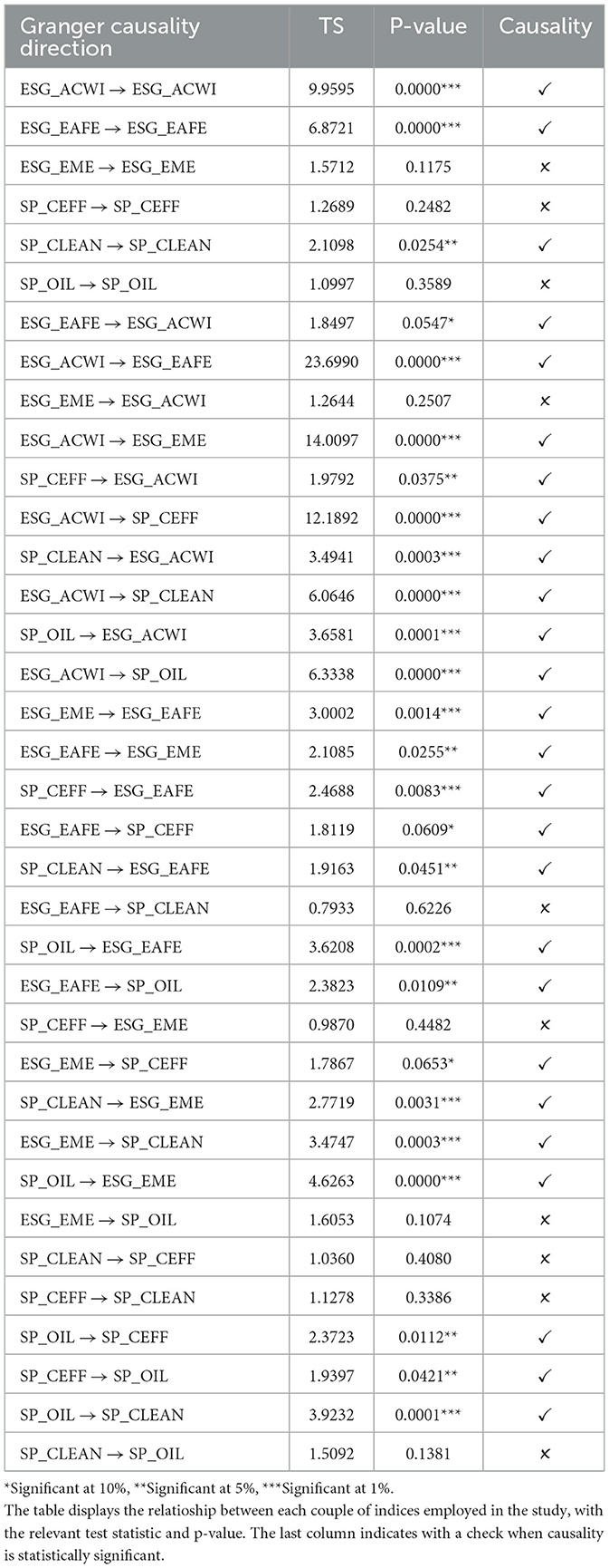
Table 6. Granger causality results.

4.2 Impulse response analysis

The relationship between IR analysis and spillover risk is that IR analysis can be used to measure and quantify the spillover effects of an economic shock or crisis. By using IR analysis, we can identify the variables that are most affected by the shock, and the magnitude and duration of the spillover effects. This can help policymakers and investors to better understand the potential risks and vulnerabilities of different economic systems, and to take appropriate actions to mitigate the spillover effects. In this article, we investigate the dynamic relationships between ESG indices in our dataset using Vector Autoregression (VAR) models. Specifically, we apply impulse response analysis to examine how each ESG index responds to a one-unit shock in the return of another ESG index and vice versa. We summarize the IR analysis of our dataset on Figure 8.

Figure 8

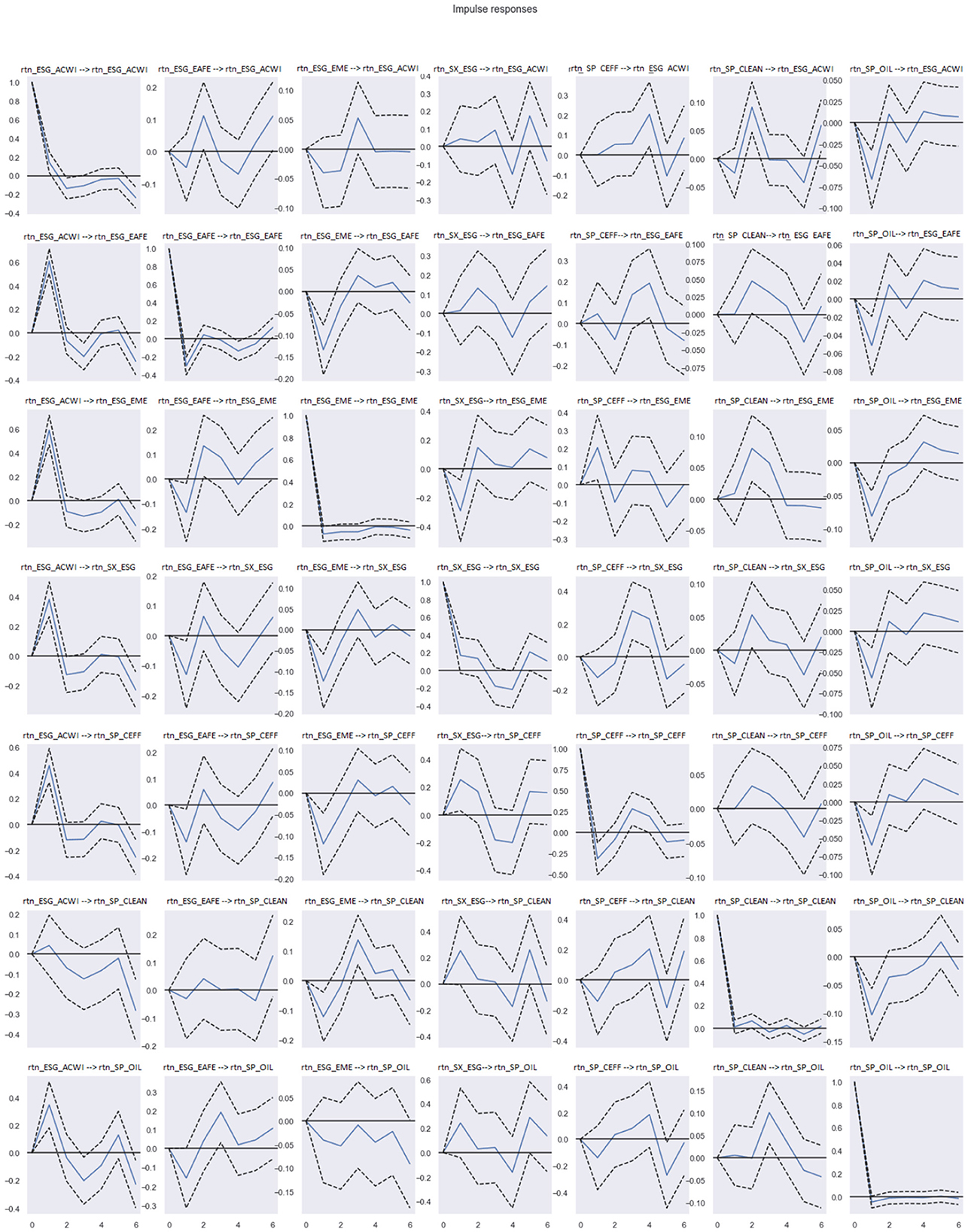
Figure 8. Impulse response analysis.

As we can see in Figure 8, one unite shock in returns on any of indices have significantly negative effect on SP_OIL, and considerably positive effect on ESG_ACWI, except whenever the shock is happened on SP_CLEAN, then the positive effect of this shock on ESG_ACWI is small. In both cases it takes at most three lags for the significant effects of the shock to dissipate. Furthermore, we can observe that a single unit shock in returns on ESG_ACWI will only become evident after two time lags. Similarly, a unit shock on ESG_EAFE will have a positive effect on SP_CLEAN, which will appear after two time lags. Similarly, the impact of a one-unit shock on SP_CEFF will be visible on SP_CLEAN after two time lags. As we can see in the Figure 8, the impact of one unit shock in SP_OIL is negative on ESG_EME for all lags. This evidence is overall consistent with the literature, e.g., Urom et al. (2022) that argues how oil prices and indexes are interrelated and that shocks propagate differently according to sector and investment horizon.

4.3 DY index

We employ the DY Index methodology (Diebold and Yilmaz, 2009, 2012) to compute the spillover index already presented in Section 3.4. We first run the function for the next 10 steps, and we obtain the “from”, “to” and “net” spillover reported in Appendix 1. Results are very similar across the steps and we, therefore, select the 10 steps ahead. Volatility Spillovers are reported in Table 7. Net spillovers show the net difference between the “contributions from others” and “contributions to others”. Accordingly, a positive net spillover implies that the specific market (index) is a net transmitter of volatility shocks, meaning it exerts more influence on other markets by sending volatility shocks. Conversely, a negative net spillover indicates that the market is a net receiver, meaning it is less affected by external markets. Among the indices included in the sample, the highest contribution to volatility spillovers is given by ESG_ACWI (380.77 including own). The second is SP_OIL.

Table 7

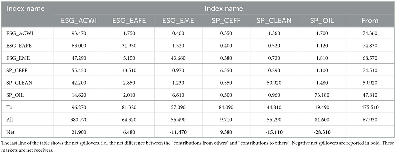
Table 7. DY volatility index results with 10 step ahead.

Volatility spillovers computed using DY index can also be represented graphically (Figure 9). The net transmitters of volatility (i.e., indices with positive net spillovers) are reported in green, and the net receivers (i.e., indices with negative net spillovers) in red. The arrows indicate the directional volatility transmission between the indices, and thinner arrows denote spillover intensities below 20. Clustering of the directional spillovers was performed using the KMeans method.

Figure 9

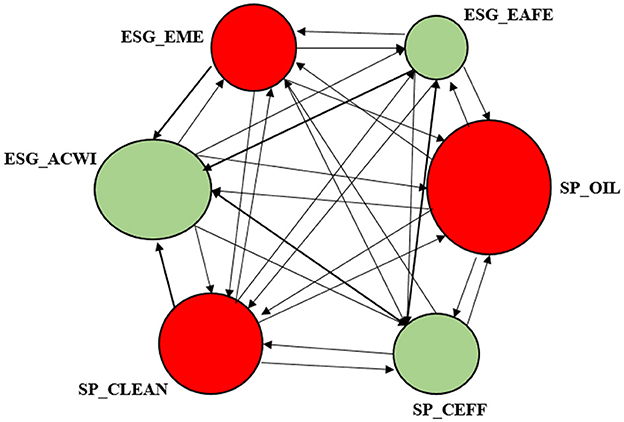
Figure 9. Volatility spillover networks using net and net pairwise spillover index.

Evidence shows that ESG_EAFE, ESG_ACVWI, our global ESG indices, and SP_CEFF are net trasmitters. While all the other indices are net receivers (red in the Figure 9). This evidence on global ESG indices is consistent with Cagli et al. (2022), but our evidence contradicts the authors' finding on Oil. According to their study, oil is a net transmitters, while we find the opposite.

5 Discussion

This study provides significant insights into the volatility spillovers among ESG equity indices and their interactions with the traditional S&P Oil index, highlighting the interconnectedness of sustainable equity markets and their vulnerability to external shocks. The findings from the Granger causality test, impulse response analysis, and Diebold-Yilmaz (DY) spillover index reveal several key patterns that align with and extend the existing literature, while also offering practical implications for investors and policymakers.

The Granger causality results (Section 4, Figure 7) show that most ESG indices exhibit bidirectional causality, indicating a high degree of interdependence. This aligns with Sahoo and Kumar (2022), who found bidirectional causality among ESG indices in BRICS markets, suggesting that ESG markets are highly integrated globally. The prominence of ESG_ACWI as a significant influencer (Table 6) may be attributed to its broad geographical coverage, encompassing both developed and emerging markets, which amplifies its role in transmitting shocks. This finding underscores the importance of global ESG benchmarks in shaping market dynamics, as noted by Gao et al. (2022), who observed a small-world structure in international ESG stock markets.

The impulse response analysis (Figure 8) further reveals that shocks to ESG indices have varied impacts. Notably, shocks to most indices positively affect ESG_ACWI but negatively impact SP_OIL, suggesting that ESG markets may respond differently to traditional energy markets during turbulent periods. This divergence is consistent with Henriques and Sadorsky (2018), who found that clean energy stock prices are more influenced by technology stocks than oil prices. The significant volatility of SP_CLEAN during 2020–2022 (Table 3, Figure 4) can be explained by its exposure to clean technology firms, which were particularly sensitive to global disruptions such as the COVID-19 pandemic and energy price fluctuations (Min, 2022). The negative response of ESG_EME to SP_OIL shocks across all lags highlights the vulnerability of emerging markets to energy market dynamics, a finding that echoes (Elsayed et al., 2020), who noted increased volatility transmission during crisis periods.

The DY spillover index results (Table 7, Figure 9) indicate that ESG_ACWI is the primary net transmitter of volatility (net spillover of 21.900), while ESG_EME and SP_CLEAN are net receivers (net spillovers of -11.470 and -15.110, respectively). This supports Cagli et al. (2022), who found that ESG indices in developed markets act as volatility transmitters to emerging markets and commodity indices. The high vulnerability of ESG_EME and SP_CLEAN can be attributed to their exposure to external shocks, such as commodity price volatility and geopolitical events (Shahzad et al., 2023). The economic rationale for this pattern lies in the structural characteristics of these markets: emerging markets often face higher macroeconomic instability, while clean technology firms are sensitive to policy changes and energy price swings.

First, the role of global ESG indices as net transmitters is consistent with the notion that large, diversified ESG portfolios (like MSCI ESG ACWI and EAFE) are more globally integrated and thus more reactive to macroeconomic shocks, geopolitical uncertainty, and climate policy news. These indices often act as a barometer for ESG sentiment, and their volatility can cascade into more sector-specific or regional indices (Bouri et al., 2022; Broadstock et al., 2021).

The result that emerging markets ESG (ESG_EME) is a net receiver supports findings in earlier studies showing that ESG markets in emerging economies tend to absorb volatility from global markets rather than transmit it (Reboredo and Ugolini, 2020). This could be due to the lower liquidity, limited ESG integration, and weaker policy enforcement in these markets.

The classification of SP_CLEAN and S&P Oil as net receivers is especially interesting. While intuitively one might expect energy-related indices to act as volatility sources—especially during periods of oil price or policy shocks—result reflects how sector-specific ESG-aligned assets may react more than lead in the volatility transmission process. This is aligned with the findings by Umar et al. (2022). Their paper shows that clean energy assets often respond to ESG and climate news from broader markets rather than initiate spillovers themselves.

These findings have several implications. For investors, the interconnectedness of ESG indices suggests that diversification benefits within ESG portfolios may be limited, particularly during crisis periods when spillovers intensify (Papathanasiou et al., 2022). Portfolio managers should consider hedging strategies to mitigate risks, especially for investments in emerging markets and clean technologies. For policymakers, the vulnerability of ESG_EME and SP_CLEAN underscores the need for targeted policies to stabilize these markets, such as subsidies for clean technology or regulatory frameworks to reduce exposure to energy price shocks. These measures are critical to supporting the transition to a sustainable economy, as emphasized by UNCTAD (2021) .

Despite its contributions, this study has limitations. The analysis is based on six indices, which may not fully capture the diversity of ESG markets. Additionally, the data extend only to June 2022, missing recent developments such as the energy crisis and monetary policy tightening. Future research could address these gaps by incorporating more indices and extending the time frame to assess the persistence of these spillover patterns.

This study enhances our understanding of ESG volatility spillovers, confirming their interdependence and highlighting the vulnerabilities of emerging markets and clean technologies. These insights are crucial for fostering sustainable investment strategies and informing policy interventions to promote greener growth.

6 Conclusions

This study investigates volatility spillovers among six ESG equity indices and the S&P Oil index, revealing complex and asymmetric interdependencies between sustainable and conventional equity markets. The analysis shows that global ESG benchmarks, such as MSCI ESG ACWI, act as key drivers of volatility, influencing both regional and sectoral indices, including those focused on clean technologies and emerging markets. These findings highlight the systemic relevance of diversified ESG portfolios and the importance of adopting a multidimensional approach to volatility modeling.

Sector-specific ESG indices, particularly those related to clean energy (SP_CLEAN) and carbon efficiency (SP_CEFF), display a heightened vulnerability to idiosyncratic shocks and tail risk, while emerging market indices reveal strong bidirectional linkages with both traditional and sustainable benchmarks. Notably, the fossil fuel market, proxied by the S&P Oil Index, continues to have significant influence on ESG asset classes. From a risk management and policy perspective, the asymmetric structure of volatility spillovers observed in this study has important implications. Investors aiming to construct resilient ESG portfolios must account for the varying dynamics of upside and downside risk, while policymakers should consider the potential for volatility contagion across sectors when designing sustainability-focused financial regulations.

However, the analysis is not without limitations. The sample period includes two major crisis episodes, the COVID-19 pandemic and the Russian invasion of Ukraine. Although recent years have continued to exhibit volatility episodes due to both economic and non-economic shocks (e.g., energy price spikes, geopolitical stress), future research should further investigate the evolution of volatility linkages across different market regimes and structural break points. The use of asymmetric volatility measures and the application of structural break tests offer promising perspectives to deepen the understanding of how systemic and idiosyncratic shocks shape the volatility transmission in ESG markets.

Data availability statement

The data analyzed in this study is subject to the following licenses/restrictions: data for this paper are used by the authors under license and cannot be redistributed. Requests to access these datasets should be directed to YWxlc3NhbmRyYS50YW5kYUB1bmlwdi5pdA==.

Author contributions

MD: Conceptualization, Writing – review & editing, Methodology, Writing – original draft. LD: Writing – review & editing, Formal analysis, Software, Conceptualization, Methodology, Supervision. FM: Formal analysis, Writing – original draft, Visualization, Methodology. AT: Conceptualization, Supervision, Writing – review & editing, Writing – original draft.

Funding

The author(s) declare that no financial support was received for the research and/or publication of this article.

Acknowledgments

MD and AT acknowledge support from CAMRisk—Centre for the Analysis and Measurement of Global Risks of the University of Pavia.

Conflict of interest

The authors declare that the research was conducted in the absence of any commercial or financial relationships that could be construed as a potential conflict of interest.

Generative AI statement

The author(s) declare that no Gen AI was used in the creation of this manuscript.

Publisher's note

All claims expressed in this article are solely those of the authors and do not necessarily represent those of their affiliated organizations, or those of the publisher, the editors and the reviewers. Any product that may be evaluated in this article, or claim that may be made by its manufacturer, is not guaranteed or endorsed by the publisher.

Supplementary material

The Supplementary Material for this article can be found online at: https://www.frontiersin.org/articles/10.3389/frsus.2025.1612279/full#supplementary-material

Footnotes

1. ^The relevance of institutional investors in the market is well testified by the holdings of global equities, that reached 43% in recent years (De La Cruz et al., 2019).

References

Abdel-Latif, H., and El-Gamal, M. (2020). Financial liquidity, geopolitics, and oil prices. Energy Econ. 87:104482. doi: 10.1016/j.eneco.2019.104482

Crossref Full Text | Google Scholar

Agosto, A., Giudici, P., and Tanda, A. (2023). How to combine ESG scores? A proposal based on credit rating prediction. Corp. Soc. Responsib. Environ. Manag. 30, 3222–3230. doi: 10.1002/csr.2458

Crossref Full Text | Google Scholar

Al-Hiyari, A., and Kolsi, M. C. (2021). How do stock market participants value ESG performance? evidence from middle eastern and north african countries. Glob. Bus. Rev. 25:9721509211001511. doi: 10.1177/09721509211001511

Crossref Full Text | Google Scholar

Andersen, T. G., and Bollerslev, T. (1998). Answering the skeptics: yes, standard volatility models do provide accurate forecasts. Int. Econ. Rev. 39, 885–905. doi: 10.2307/2527343

Crossref Full Text | Google Scholar

Asafu-Adjaye, J. (2000). The relationship between energy consumption, energy prices and economic growth: time series evidence from asian developing countries. Energy Econ. 22, 615–625. doi: 10.1016/S0140-9883(00)00050-5

Crossref Full Text | Google Scholar

Ballestero, E., Bravo, M., Pérez-Gladish, B., Arenas-Parra, M., and Pla-Santamaria, D. (2012). Socially responsible investment: a multicriteria approach to portfolio selection combining ethical and financial objectives. Eur. J. Oper. Res. 216, 487–494. doi: 10.1016/j.ejor.2011.07.011

Crossref Full Text | Google Scholar

Barndorff-Nielsen, O. L., Kinnebrock, S., and Shephard, N. (2010). “Measuring downside risk of realized semivariance,” in Volatility and Time Series Econometrics: Essays in Honor of Robert F. eds. T. Bollerslev, J. Russell and M. Watson (Oxford: Oxford University Press), 117–136.

Google Scholar

Barrett, A. B., Barnett, L., and Seth, A. K. (2010). Multivariate granger causality and generalized variance. Phys. Rev. E 81:41907. doi: 10.1103/PhysRevE.81.041907

PubMed Abstract | Crossref Full Text | Google Scholar

Baruník, J., and Křehlík, T. (2018). Measuring the frequency dynamics of financial connectedness and systemic risk. J. Financ. Econom. 16, 271–296. doi: 10.1093/jjfinec/nby001

Crossref Full Text | Google Scholar

Bollen, J., Mao, H., and Zeng, X. (2011). Twitter mood predicts the stock market. J. Comput. Sci. 2, 1–8. doi: 10.1016/j.jocs.2010.12.007

Crossref Full Text | Google Scholar

Bouri, E., Iqbal, N., and Klein, T. (2022). Climate policy uncertainty and the price dynamics of green and brown energy stocks. Financ. Res. Lett. 47:102740. doi: 10.1016/j.frl.2022.102740

Crossref Full Text | Google Scholar

Broadstock, D. C., Chan, K., Cheng, L. T., and Wang, X. (2021). The role of ESG performance during times of financial crisis: evidence from COVID-19 in China. Financ. Res. Lett. 38:101716. doi: 10.1016/j.frl.2020.101716

PubMed Abstract | Crossref Full Text | Google Scholar

Cagli, E. C. C., Mandaci, P. E., and Taşkın, D. (2022). Environmental, social, and governance (ESG) investing and commodities: dynamic connectedness and risk management strategies. Sustain. Account. Manag. Policy J. 14, 1052–1074. doi: 10.1108/SAMPJ-01-2022-0014

Crossref Full Text | Google Scholar

Carlsson Hauff, J., and Nilsson, J. (2023). Is ESG mutual fund quality in the eye of the beholder? An experimental study of investor responses to ESG fund strategies. Bus. Strat. Environ. 32, 1189–1202. doi: 10.1002/bse.3181

Crossref Full Text | Google Scholar

Cerqueti, R., Ciciretti, R., Dalò, A., and Nicolosi, M. (2021). Esg investing: a chance to reduce systemic risk. J. Financ. Stabil. 54:100887. doi: 10.1016/j.jfs.2021.100887

Crossref Full Text | Google Scholar

De La Cruz, A., Medina, A., and Tang, Y. (2019). Owners of the World's Listed Companies. OECD Capital Market Series: Paris.

Google Scholar

Deloitte. (2024). How can the enterprise earn investor trust through sustainability disclosures? Technical Report, London.

Google Scholar

Diebold, F. X., and Yilmaz, K. (2009). Measuring financial asset return and volatility spillovers, with application to global equity markets. Econ. J. 119, 158–171. doi: 10.1111/j.1468-0297.2008.02208.x

Crossref Full Text | Google Scholar

Diebold, F. X., and Yilmaz, K. (2012). Better to give than to receive: predictive directional measurement of volatility spillovers. Int. J. Forecast. 28, 57–66. doi: 10.1016/j.ijforecast.2011.02.006

Crossref Full Text | Google Scholar

Diebold, F. X., and Yilmaz, K. (2014). On the network topology of variance decompositions: measuring the connectedness of financial firms. J. Econometr. 182, 119–134. doi: 10.1016/j.jeconom.2014.04.012

Crossref Full Text | Google Scholar

Dutta, A., and Hasib Noor, M. (2017). Oil and non-energy commodity markets: an empirical analysis of volatility spillovers and hedging effectiveness. Cogent Econ. Finance 5:1324555. doi: 10.1080/23322039.2017.1324555

Crossref Full Text | Google Scholar

Elsayed, A. H., Nasreen, S., and Tiwari, A. K. (2020). Time-varying co-movements between energy market and global financial markets: implication for portfolio diversification and hedging strategies. Energy Econ. 90:104847. doi: 10.1016/j.eneco.2020.104847

Crossref Full Text | Google Scholar

Ferrer, R., Shahzad, S. J. H., López, R., and Jareño, F. (2018). Time and frequency dynamics of connectedness between renewable energy stocks and crude oil prices. Energy Econ. 76, 1–20. doi: 10.1016/j.eneco.2018.09.022

Crossref Full Text | Google Scholar

Gao, Y., Li, Y., Zhao, C., and Wang, Y. (2022). Risk spillover analysis across worldwide esg stock markets: new evidence from the frequency-domain. N. Am. J. Econ. Finance 59:101619. doi: 10.1016/j.najef.2021.101619

Crossref Full Text | Google Scholar

Giese, G., Lee, L.-E., Melas, D., Nagy, Z., and Nishikawa, L. (2019). Foundations of ESG investing: how ESG affects equity valuation, risk, and performance. J. Portf. Manag. 45, 69–83. doi: 10.3905/jpm.2019.45.5.069

Crossref Full Text | Google Scholar

Global Sustainable Investment Alliance (2021). Global Sustainable Investment Review 2020. Brussels.

Google Scholar

Global Sustainable Investment Alliance (2023). Global Sustainable Investment Review 2022. Technical Report. Brussels: GSIA.

Google Scholar

Granger, C. W. (1969). Investigating causal relations by econometric models and cross-spectral methods. Econometrica 37, 424–438. doi: 10.2307/1912791

Crossref Full Text | Google Scholar

Henriques, I., and Sadorsky, P. (2018). Investor implications of divesting from fossil fuels. Glob. Finance J. 38, 30–44. doi: 10.1016/j.gfj.2017.10.004

Crossref Full Text | Google Scholar

IIA (2022). IIA's Second Annual Global ESG Asset Manager Survey. Technical Report, Index Industry Association.

Google Scholar

Karoui, A., and Nguyen, D. K. (2022). Systematic esg exposure and stock returns: evidence from the united states during the 1991–2019 period. Bus. Ethics Environ. Respons. 31, 604–619. doi: 10.1111/beer.12429

Crossref Full Text | Google Scholar

Kassim, S. H., Majid, M. S. A., and Yusof, R. M. (2009). Impact of monetary policy shocks on the conventional and islamic banks in a dual banking system: evidence from malaysia. J. Econ. Coop. Dev. 30, 41–58. Available online at: https://www.sesric.org/publications-jecd-articles.php?jec_id=69

Google Scholar

Khalfaoui, R., Solarin, S. A., Al-Qadasi, A., and Ben Jabeur, S. (2022). Dynamic causality interplay from COVID-19 pandemic to oil price, stock market, and economic policy uncertainty: evidence from oil-importing and oil-exporting countries. Ann. Oper. Res. 313, 105–143. doi: 10.1007/s10479-021-04446-w

PubMed Abstract | Crossref Full Text | Google Scholar

Killick, R., Fearnhead, P., and Eckley, I. A. (2012). Optimal detection of changepoints with a linear computational cost. J. Am. Stat. Assoc. 107, 1590–1598. doi: 10.1080/01621459.2012.737745

Crossref Full Text | Google Scholar

Kumar, S., Managi, S., and Matsuda, A. (2012). Stock prices of clean energy firms, oil and carbon markets: a vector autoregressive analysis. Energy Econ. 34, 215–226. doi: 10.1016/j.eneco.2011.03.002

Crossref Full Text | Google Scholar

Lütkepohl, H. (2010). Impulse Response Function. Springer: New York. doi: 10.1057/9780230280830_16

Crossref Full Text | Google Scholar

Masih, R., Peters, S., and De Mello, L. (2011). Oil price volatility and stock price fluctuations in an emerging market: evidence from south korea. Energy Econ. 33, 975–986. doi: 10.1016/j.eneco.2011.03.015

Crossref Full Text | Google Scholar

Min, H. (2022). Examining the impact of energy price volatility on commodity prices from energy supply chain perspectives. Energies 15:7957. doi: 10.3390/en15217957

Crossref Full Text | Google Scholar

Morningstar. (2024). Global ESG Funds Hit by Outflows for First Time in Q4 2023. Chicago, IL: Sustainable Investments.

Google Scholar

Papathanasiou, S., Dokas, I., and Koutsokostas, D. (2022). Value investing versus other investment strategies: a volatility spillover approach and portfolio hedging strategies for investors. N. Am. J. Econ. Finance 62:101764. doi: 10.1016/j.najef.2022.101764

Crossref Full Text | Google Scholar

Petelczyc, J. (2022). The readiness for ESG among retail investors in central and eastern europe. The example of poland. Glob. Bus. Rev. 23, 1299–1315. doi: 10.1177/09721509221114754

Crossref Full Text | Google Scholar

Reboredo, J. C., Rivera-Castro, M. A., and Ugolini, A. (2017). Wavelet-based test of co-movement and causality between oil and renewable energy stock prices. Energy Econ. 61, 241–252. doi: 10.1016/j.eneco.2016.10.015

Crossref Full Text | Google Scholar

Reboredo, J. C., and Ugolini, A. (2018). The impact of energy prices on clean energy stock prices. A multivariate quantile dependence approach. Energy Econ. 76, 136–152. doi: 10.1016/j.eneco.2018.10.012

Crossref Full Text | Google Scholar

Reboredo, J. C., and Ugolini, A. (2020). Price connectedness between green bond and financial markets. Econ. Model. 88, 25–38. doi: 10.1016/j.econmod.2019.09.004

Crossref Full Text | Google Scholar

Reboredo, J. C., Ugolini, A., and Chen, Y. (2019). Interdependence between renewable-energy and low-carbon stock prices. Energies 12:4461. doi: 10.3390/en12234461

Crossref Full Text | Google Scholar

Sabbaghi, O. (2023). ESG and volatility risk: international evidence. Bus. Ethics Environ. Respons. 32, 802–818. doi: 10.1111/beer.12512

Crossref Full Text | Google Scholar

Sadorsky, P. (2012). Correlations and volatility spillovers between oil prices and the stock prices of clean energy and technology companies. Energy Econ. 34, 248–255. doi: 10.1016/j.eneco.2011.03.006

Crossref Full Text | Google Scholar

Sahoo, S., and Kumar, S. (2022). Integration and volatility spillover among environmental, social and governance indices: evidence from brics countries. Glob. Bus. Rev. 23, 1280–1298. doi: 10.1177/09721509221114699

Crossref Full Text | Google Scholar

Shahzad, U., Mohammed, K. S., Tiwari, S., Nakonieczny, J., and Nesterowicz, R. (2023). Connectedness between geopolitical risk, financial instability indices and precious metals markets: novel findings from russia ukraine conflict perspective. Resour. Policy 80:103190. doi: 10.1016/j.resourpol.2022.103190

Crossref Full Text | Google Scholar

Sharma, G. D., Sarker, T., Rao, A., Talan, G., and Jain, M. (2022). Revisiting conventional and green finance spillover in post-covid world: evidence from robust econometric models. Glob. Finance J. 51:100691. doi: 10.1016/j.gfj.2021.100691

Crossref Full Text | Google Scholar

Škare, M., Blažević Burić, S., and Sinković, D. (2022). Effects of energy prices shocks on global inflation: a panel structural var approach. Acta Montan. Slov. 27, 929–943. doi: 10.46544/AMS.v27i4.08

Crossref Full Text | Google Scholar

Townsend, B. (2020). From SRI to ESG: the origins of socially responsible and sustainable investing. J. Impact ESG Invest. 1, 10–25. doi: 10.3905/jesg.2020.1.1.010

Crossref Full Text | Google Scholar

Umar, Z., Yousaf, I., Gubareva, M., and Vo, X. V. (2022). Spillover and risk transmission between the term structure of the us interest rates and islamic equities. Pac.-Bas. Finance J. 72:101712. doi: 10.1016/j.pacfin.2022.101712

Crossref Full Text | Google Scholar

UNCTAD (2021). The Rise of the Sustainable Fund Market and its Role in Financing Sustainable Development. Geneve.

Google Scholar

Ur Rehman, R., Zhang, J., Uppal, J., Cullinan, C., and Akram Naseem, M. (2016). Are environmental social governance equity indices a better choice for investors? An asian perspective. Bus. Ethics Eur. Rev. 25, 440–459. doi: 10.1111/beer.12127

Crossref Full Text | Google Scholar

Urom, C., Mzoughi, H., Ndubuisi, G., and Guesmi, K. (2022). Directional predictability and time-frequency spillovers among clean energy sectors and oil price uncertainty. Q. Rev. Econ. Finance 85, 326–341. doi: 10.1016/j.qref.2022.04.005

Crossref Full Text | Google Scholar