Reference Ellipsoid and Geoid in Chronometric Geodesy

1. Introduction

Accurate definition, determination and realization of terrestrial reference frame is essential for fundamental astronomy, celestial mechanics, geophysics as well as for precise satellite and aircraft navigation, positioning, and mapping. The International Terrestrial Reference Frame (ITRF) is materialized by coordinates of a number of geodetic points (stations) located on the Earth's surface, and spread out across the globe. Definition of the coordinates is derived from the International Terrestrial Reference System (ITRS) which is a theoretical concept. ITRF is used to measure plate tectonics, regional subsidence or loading and to describe the Earth's rotation in space by measuring its rotational parameters (Petit and Luzum, 2010).

Nowadays, four main geodetic techniques are used to compute the accurate terrestrial coordinates and velocities of stations—GPS, VLBI, SLR, and DORIS, for the realization of ITRF. The observations are so accurate that geodesists have to model and include to the data processing the secular Earth's crust changes to reach self-consistency between the various ITRF realizations referred to different epoch. It is recognized that in order to maintain the up-to-date ITRF realization as accurate as possible the development of the most precise theoretical model and relationships between parameters of the model is of a paramount importance.

This model is not of a pure kinematic origin because the gravity field plays an essential role in geodetic network computations (Heiskanen and Moritz, 1967; Hofmann-Wellenhof and Moritz, 2006) making a particular theory of gravity a part of definition of the ITRS. Until recently, such a theory was the Newtonian theory of gravity. However, current SLR/GPS/VLBI techniques allow us to determine the transformation parameters between the coordinates and velocities of the collocation points of the ITRF realization with the precision approaching to ~1 mm and ~1 mm/year, respectively (Petit and Luzum, 2010, Table 4.1). At the same time, general relativity predicts that the post-Newtonian effects in measuring the ITRF coordinates, as compared with the Newtonian theory of gravity, is of the order of the Earth's gravitational radius that is about 1 cm (Kopejkin, 1991; Müller et al., 2008). This general-relativistic effect distorts the coordinate grid of ITRF at the noticeable level which can be detected with the currently available geodetic techniques and, hence, should be taken into account.

ITRS is specified by the Cartesian equatorial coordinates rotating rigidly with the Earth. For the purposes of geodesy and gravimetry the Cartesian coordinates are often converted to a geographical system of elliptical coordinates (h, θ, λ) referred to an international reference ellipsoid which is a non-trivial solution of the Newtonian gravity field equations found by Maclaurin (Chandrasekhar, 1967). It describes the figure of a fluid body with a homogeneous mass density rotating around a fixed z-axis with a constant angular velocity ω. The post-Newtonian effects deforms the shape of Maclaurin's ellipsoid (Chandrasekhar, 1965; Bardeen, 1971) and modify the basic equations of classic geodesy (Müller et al., 2008; Kopeikin et al., 2011, 2016). These relativistic effects must be properly calculated to ensure the adequacy of the geodetic coordinate transformations at the millimeter level of accuracy. A pioneering study of relativistic effects in geodesy have been carried out by Bjerhammar (1985).

Post-Newtonian equilibrium configurations of uniformly rotating fluids have been discussed in literature by researchers from USA (Chandrasekhar, 1965, 1967a,b,c, 1971a,b; Bardeen, 1971; Chandrasekhar and Elbert, 1974, 1978; Chandrasekhar and Miller, 1974), Lithuania (Bondarenko and Pyragas, 1974; Pyragas et al., 1974, 1975), USSR (Tsirulev and Tsvetkov, 1982a,b; Tsvetkov and Tsirulev, 1983; Galtsov et al., 1984) and, the most recently, scientists from the Fridrich Schiller University of Jena in Germany (Petroff, 2003; Ansorg et al., 2004; Meinel et al., 2008; Gürlebeck and Petroff, 2010, 2013). These papers focused primarily on studying the astrophysical aspects of the problem like stability of the rotating stars, the points of bifurcations, exact axially-symmetric spacetimes, emission of gravitational waves, etc. The present paper focuses on the post-Newtonian effects in physical geodesy. More specifically, we extend the research on the figures of equilibrium into the realm of relativistic geodesy and pay attention to the possible geodetic applications for the adequate processing of the high-precise data obtained by various geodetic techniques that include but not limited to SLR, LLR, VLBI, DORIS, and GNSS (Drewes, 2009; Plag and Pearlman, 2009).

Important stimulating factor for pursuing more advanced theoretical research on relativistic effects in geodesy and the Earth figure of equilibrium is related to the recent breakthrough in manufacturing ring laser gyroscopes (Schreiber, 2013; Beverini et al., 2014; Hurst et al., 2015). Earth rotation and orientation provide the link between the terrestrial (ITRF) and celestial reference frames (ICRF). Traditionally, the Earth orientation parameters (EOPs) are observed by the International Earth Rotation Service (IERS) that operates the global VLBI network. VLBI technique determines EOPs off-line after accumulating the data over sufficiently long period of time. Moreover, VLBI depends on suitable models of Earth's troposphere and geophysical factors which are difficult to predict. Ring laser gyroscopes provide direct access to the Earth rotation axis and a high resolution in the short-term. Currently, the modern quantum optics has matured to a point where the ring laser gyroscopes can resolve rotation rates of 10⁻¹² rad/s after 1 h of integration and demonstrate an impressive stability over several month (Schreiber, 2013). The combination of VLBI and ring laser measurements offers an improved sensitivity for the EOPs in the short-term and the direct access to the Earth rotation axis. Another application of the ring laser gyroscopes is to measure the Lense-Thirring effect predicted by Einstein's general relativity (Ciufolini and Wheeler, 1995), in a terrestrial laboratory environment (Beverini et al., 2014).

Another, rapidly emerging branch of relativistic geodesy is called chronometric geodesy (Petit et al., 2014). This new line of development is pushed forward by the fascinating progress in making up quantum clocks (Poli et al., 2013), ultra-precise time-scale dissemination over the globe (Kómár et al., 2014), and geophysical applications of the clocks (Bondarescu et al., 2012, 2015). Clocks at rest in a gravitational potential tick slower than clocks outside of it. On Earth, this translates to a relative frequency change of 10⁻¹⁶ per meter of height difference (Falke et al., 2014). Comparing the frequency of a probe clock with a reference clock provides a direct measure of the gravity potential difference between the two clocks. This novel technique has been dubbed chronometric leveling. It is envisioned as one of the most promising application of the relativistic geodesy in a near future (Mai and Müller, 2013; Mai, 2014; Petit et al., 2014). Optical frequency standards have recently reached stability of 2.2 × 10⁻¹⁶ at 1 s, and demonstrated an overall fractional frequency uncertainty of 2.1 × 10⁻¹⁸ (Nicholson et al., 2015) which enables their use for chronometric geodesy at the absolute level of one centimeter.

The chronometric leveling directly measures the equipotential surface of gravity field (geoid) without conducting a complicated gravimetric survey and solving the differential equations for the anomalous gravity potentials (Stoke's or Molodensky's problem Hofmann-Wellenhof and Moritz, 2006; Torge and Müller, 2012). Combining the data of the chronometric leveling with those of the conventional geodetic techniques will allow us to determine the normal heights of reference points with an unprecedented accuracy (Bondarescu et al., 2012). An adequate physical interpretation of this type of measurements requires more precise theoretical definition of geoid (Kopeikin et al., 2015; Oltean et al., 2015) and is inconceivable without an accompanying development of the corresponding mathematical algorithms accounting for the major relativistic effects in the description of the equipotential level surface and its, so-called, normal) gravity field (Hofmann-Wellenhof and Moritz, 2006; Torge and Müller, 2012).

The objective of the present paper is to suggest a solution of Einstein's gravity field equations that gives rise to the post-Newtonian equipotential surface described by the second-order polynomial which exactly coincides with the shape of the Maclaurin ellipsoid in the Newtonian gravity. Our previous paper (Kopeikin et al., 2016) has explored the post-Newtonian case of a homogeneous density distribution of a uniformly rotating perfect fluid. We have shown that the post-Newtonian effects inevitably distort the Maclaurin ellipsoid of rotation to a surface described by the fourth-order polynomial which cannot be reduced to the ellipsoidal surface of the second order by doing coordinate transformations. In the present paper we assume that the mass distribution is not homogeneous but an ellipsoidal one with a free parameter, and prove that under this assumption the equipotential level surface can be made as an exact ellipsoid of the second order which may be found more convenient for doing the reduction of high-precise geodetic measurements with taking into account relativistic corrections.

The paper consists of several sections, bibliography and appendix. Section 2 explains briefly the principles of the post-Newtonian approximations and describes the post-Newtonian metric tensor. In Section 3 we give definition of the post-Newtonian geoid. Section 4 discusses the post-Newtonian ellipsoid which generalizes the Maclaurin ellipsoid and is, in general, the surface of the fourth order. It also introduces the reader to the concept of the post-Newtonian coordinate freedom and shows how this freedom can be used to simplify the mathematical description of the PN-ellipsoid. Sections 5–7 calculate respectively the Newtonian and post-Newtonian gravitational potentials inside the rotating PN-ellipsoid. Sections 8, 9 give the post-Newtonian definitions of the conserved mass and angular momentum. Section 10 derives the post-Newtonian equations of the equipotential level surface. Sections 11, 12 provide the reader with the relativistic generalization of the Pizzetti and Clairaut theorem of classical geodesy (Pizzetti, 1913). Section 13 approximates the relativistic formulas which can be used in practical applications of relativistic geodesy and shows how to build the exact reference-ellipsoid in the post-Newtonian approximation. Finally, Section 14 introduces the concept of the post-Newtonian geoid's undulation and its relation to the current problem of the measurement of the global average sea level. Appendix contains technical details of calculations of the mathematical integrals which appear in the main part of the paper.

The following notations are used throughout the paper:

• the Greek indices α, β, … run from 0 to 3,

• the Roman indices i, j, … run from 1 to 3,

• repeated Greek indices mean Einstein's summation from 0 to 3,

• repeated Roman indices mean Einstein's summation from 1 to 3,

• the unit matrix (also known as the Kroneker symbol) is denoted by ${\delta }_{ij}={\delta }^{ij}$,

• the fully antisymmetric symbol Levi-Civita is denoted as ${\epsilon }_{ijk}={\epsilon }^{ijk}$ with ε₁₂₃ = + 1,

• the bold letters a = (a¹, a², a³) ≡ (aⁱ), b = (b¹, b², b³) ≡ (bⁱ), and so on, denote spatial 3-dimensional vectors,

• a dot between two spatial vectors, for example $a·b=a^1{b}^1+a^2{b}^2+a^3{b}^3={\delta }_{ij}{a}^i{b}^j$, means the Euclidean dot product,

• the cross between two vectors, for example (a × b)ⁱ ≡ ε^ijka^jb^k, means the Euclidean cross product,

• we use a shorthand notation for partial derivatives ${\partial }_{\alpha }=\partial ∕\partial x^{\alpha }$,

• covariant derivative with respect to a coordinate x^α is denoted as ∇_α;

• the Minkowski (flat) space-time metric η_αβ = diag(−1, +1, +1, +1),

• g_αβ is the physical spacetime metric,

• ḡ_αβ is the background spacetime metric describing the gravitational field of the reference ellipsoid,

• the Greek indices are raised and lowered with the metric ḡ_αβ,

• G is the universal gravitational constant,

• c is the speed of light in vacuum,

• ω is a constant rotational velocity,

• ρ is a bare constant density of the fluid,

• a is a semi-major axis of the ellipsoid of revolution,

• b is a semi-minor axis of the ellipsoid of revolution,

• ρ₀ is a constant bare density of matter,

• $\kappa \equiv \pi G{\rho }_0{a}^2∕c^2$ is a dimensional parameter characterizing the strength of gravitational field,

• a bar above any quantity indicates that it belongs to the background spacetime manifold with the metric ḡ_αβ.

Other notations are explained in the text as they appear.

2. Post-Newtonian Spacetime and Metric Tensor

Discussion of the chronometric geodesy starts from the construction of the spacetime manifold for the case of a rotating Earth. We shall employ Einstein's general relativity to build such a manifold though some other alternative theories of gravity discussed, for example in Will (1993), can be used as well. Einstein's field equations represent a system of ten non-linear differential equations in partial derivatives for the ten components of the metric tensor, g_αβ, which represent gravitational potentials. Because the equations are difficult to solve exactly due to their non-linearity, we apply the post-Newtonian approximations (PNA) for their solution (Chandrasekhar, 1965).

The PNA are applied in case of slowly-moving matter having a weak gravitational field. This is exactly the situation in the solar system which makes PNA highly appropriate for constructing relativistic theory of reference frames (Soffel et al., 2003) and relativistic celestial mechanics in the solar system (Soffel, 1989; Brumberg, 1991; Kopeikin et al., 2011). The PNA are based on the assumption that a Taylor expansion of the metric tensor can be done in the inverse powers of the speed of gravity c that is equal to the speed of light in vacuum in general relativity. Exact mathematical formulation of a set of basic axioms required for doing the post-Newtonian expansion was given by Rendall (1990). Practically, it requires to have several small parameters characterizing the source of gravity. They are: ε_i ~ v_i ∕ c, ε_e ~ v_e ∕ c, and ${\eta }_i~U_i∕c^2$, ${\eta }_e~U_e∕c^2$, where v_i is a characteristic velocity of motion of matter inside a body, v_e is a characteristic velocity of the relative motion of the bodies with respect to each other, U_i is the internal gravitational potential of each body, and U_e is the external gravitational potential between the bodies. If one denotes a characteristic radius of a body as L and a characteristic distance between the bodies as R, the internal and external gravitational potentials will be U_i ≃ GM ∕ L and U_e ≃ GM ∕ R, where M is a characteristic mass of the body. Due to the virial theorem of the Newtonian gravity (Chandrasekhar, 1965) the small parameters are not independent. Specifically, one has ${\epsilon }_i^2~{\eta }_i$ and ${\epsilon }_e^2~{\eta }_e$. Hence, parameters ε_i and ε_e are sufficient in doing post-Newtonian approximations. Because within the solar system these parameters do not significantly differ from each other, we shall not distinguished them. Quite often we shall use notation κ ≡ πGρa² ∕ c² to mark the powers of the fundamental speed c in the post-Newtonian terms.

We assume that physical spacetime has the metric tensor denoted as g_αβ. This spacetime is well-approximated by a background manifold with the metric tensor denoted ḡ_αβ. The perturbation of gravitational field is denoted with ϰ_αβ and is called the anomalous gravity potential. We, first, build the metric tensor of the background manifold by solving Einstein's equations in harmonic coordinates x^α = (x⁰, xⁱ), where x⁰ = ct, and t is the coordinate time. The class of the harmonic coordinates is defined by imposing the de Donder gauge condition on the metric tensor (Fock, 1964; Weinberg, 1972),

$\begin{array}{ll}{\partial }_{\alpha }\left(\sqrt{-ḡ}{ḡ}^{\alpha \beta }\right)=0.& (1)\end{array}$

Einstein equations for the metric tensor are a complicated non-linear system of differential equations in partial derivatives. Because gravitational field of the solar system is weak and motion of matter is slow, we focus on the first post-Newtonian approximation of general relativity. We also assume that the source of the background metric is a perfect fluid. Under these assumptions the post-Newtonian background metric has the following form (Kopeikin et al., 2011)

$\begin{array}{rc}{ḡ}_{00}=-1+\frac{2\bar{V}}{c^2}+\frac{2}{c^4}\left(\bar{\Phi }-{\bar{V}}^2\right)+{O}\left(c^{-6}\right),& (2)\end{array}$

$\begin{array}{rc}{ḡ}_{0i}=-\frac{4{\bar{V}}^i}{c^3}+{O}\left(c^{-5}\right),& (3)\end{array}$

$\begin{array}{rc}{ḡ}_{ij}={\delta }_{ij}\left(1+\frac{2\bar{V}}{c^2}\right)+{O}\left(c^{-4}\right),& (4)\end{array}$

where the gravitational potentials entering the metric, satisfy the Poisson equations,

$\begin{array}{rc}\Delta \bar{V}=-4\pi G\bar{\rho },& (5)\end{array}$

$\begin{array}{rc}\Delta {\bar{V}}^i=-4\pi G\bar{\rho }{v}^i,& (6)\end{array}$

$\begin{array}{rc}\Delta \bar{\Phi }=-4\pi G\bar{\rho }\left(2v^2+2\bar{V}+\bar{\Pi }+\frac{3\bar{p}}{\bar{\rho }}\right),& (7)\end{array}$

with $\overline{p}$ and vⁱ being pressure and velocity of matter respectively, and $\overline{\Pi }$ is the internal energy of matter per unit mass. We emphasize that $\overline{\rho }$ is the local mass density of baryons per a unit of invariant (3-dimensional) volume element $dV=\sqrt{-ḡ}{u}^0{d}^{3}x$, where u⁰ is the time component of the 4-velocity of matter. The local mass density, $\overline{\rho }$, relates in the post-Newtonian approximation to the invariant mass density ${\overline{\rho }}^{*}=\sqrt{-ḡ}{u}^0\overline{\rho }$, namely (Kopeikin et al., 2011)

$\begin{array}{ll}{\bar{\rho }}^{*}=\bar{\rho }+\frac{\bar{\rho }}{c^2}\left(\frac{1}{2}{v}^2+3\bar{V}\right).& (8)\end{array}$

The internal energy, $\overline{\Pi }$, is related to pressure, $\overline{p}$, and the local density, $\overline{\rho }$, through the thermodynamic equation

$\begin{array}{ll}d\bar{\Pi }+\bar{p}d\left(\frac{1}{\bar{\rho }}\right)=0,& (9)\end{array}$

and the equation of state, $\overline{p}=\overline{p}(\overline{\rho })$.

We shall further assume that the background matter rotates rigidly around fixed z axis with a constant angular velocity ω. This makes the background spacetime stationary with the background metric being independent on time. In the stationary spacetime, the mass density ρ* obeys the exact equation of continuity

$\begin{array}{ll}{\partial }_i\left({\bar{\rho }}^{*}{v}^i\right)=0.& (10)\end{array}$

Velocity of rigidly rotating fluid is

$\begin{array}{ll}{v}^i={\epsilon }^{ijk}{\omega }^j{x}^k,& (11)\end{array}$

where ωⁱ = (0, 0, ω) is the constant angular velocity. Replacing velocity vⁱ in Equation (10) with Equation (11), and differentiating, reveals that

$\begin{array}{ll}{v}^i{\partial }_i\bar{\rho }=0,& (12)\end{array}$

which means that velocity of the fluid is tangent to the surfaces of a constant density $\overline{\rho }$.

3. Relativistic Geoid

The Newtonian concept of Earth's geoid was extended to the post-Newtonian approximation of general relativity in Soffel (1989) and Kopejkin (1991). Exact concept of the relativistic geoid in general relativity that is not limited to the first post-Newtonian approximation has been discussed in Kopeikin et al. (2015) and Oltean et al. (2015).

We consider the Earth as made up of the background matter with small perturbations which reflect the actual mass distribution, stresses, and velocity flow of Earth's matter with respect to the rigidly rotating frame of reference. The angular velocity, ω, of Earth's rotation also slowly changes because of precession, nutation, polar motion and variations in the length-of-day. The physical metric, g_αβ, depends on time and spatial coordinates. It is decomposed into an algebraic sum of the background metric ḡ_αβ, and its perturbation, ϰ_αβ,

$\begin{array}{ll}{g}_{\alpha \beta }={ḡ}_{\alpha \beta }+{\varkappa }_{\alpha \beta }.& (13)\end{array}$

In the present paper, we shall neglect dependence of the perturbation ϰ_αβ on time because it produces very tiny relativistic effects that are currently unobservable.

Terrestrial reference frame is formed by the world lines of observers being fixed with respect to the crust of the Earth. Each observer moves in spacetime with four-velocity u^α = c⁻¹dx^α ∕ dτ where x^α = {x⁰, x¹, x², x³} are coordinates of the observer, and τ is its proper time defined in terms of the metric tensor Equation (13) as follows,

$\begin{array}{ll}{c}^{2}d{\tau }^2=-g_{\alpha \beta }d{x}^{\alpha }d{x}^{\beta }.& (14)\end{array}$

Physical space of observers at each instant of time is represented by a three-dimensional hypersurface of constant proper time that is orthogonal everywhere to the world lines of the observers. The metric tensor on this hypersurface is denoted as h_αβ and is given by Zelmanov et al. (2006) and Landau and Lifshitz (1975)

$\begin{array}{ll}{h}_{\alpha \beta }\equiv g_{\alpha \beta }+u_{\alpha }{u}_{\beta }.& (15)\end{array}$

It is used to measure the spatial distances. Rising and lowering of Greek indices of geometric objects residing on the perturbed manifold are done with the help of the full metric g_αβ.

Similarly to classic geodesy, general relativity offers two definitions of relativistic geoid (Soffel, 1989; Kopejkin, 1991)

Definition 1: The relativistic u-geoid represents a two-dimensional surface at any point of which the rate of the proper time, τ, of an ideal clock carried out by a set of fiducial terrestrial observers is constant.

The u-geoid is determined by equation W = const., where the physical gravity potential

$\begin{array}{ll}W(x)=c^2\left(1-\frac{d\tau }{dt}\right).& (16)\end{array}$

Because $d\tau ∕dt=\sqrt{-g_{\alpha \beta }{ẋ}^{\alpha }{ẋ}^{\beta }}$, where the dot means the total time derivative with respect to the coordinate time t, Equation (16) becomes,

$\begin{array}{ll}W(x)\equiv c^2\left[1-{\left(-g_{00}-\frac{2}{c}{g}_{0i}{v}^i-\frac{1}{c^2}{g}_{ij}{v}^i{v}^j\right)}^{1∕2}\right].& (17)\end{array}$

This matches the Newtonian definition of the geoid after decomposition of the metric tensor in the post-Newtonian series and discarding all post-Newtonian terms.

Definition 2: The relativistic a-geoid represents a two-dimensional surface at any point of which the direction of a plumb line measured by the terrestrial observer, is orthogonal to the tangent plane of geoid's surface.

In order to derive equation of a-geoid, we notice that the direction of the plumb line is given by a four-vector of the physical acceleration of gravity, $g_{\alpha }\equiv -c^2{a}_{\alpha }$ where $a_{\alpha }=u^{\beta }{\nabla }_{\beta }{u}_{\alpha }$ is a four-acceleration of the terrestrial observer being orthogonal to u^α. In case of a stationary rotating configuration of matter, we get (Lightman et al., 1975, Problems 10.14 and 16.17)

$\begin{array}{ll}{g}_{\alpha }=-c^2{\partial }_{\alpha }ln\left(1-\frac{W}{c^2}\right),& (18)\end{array}$

where W is calculated in Equation (17). We consider an arbitrary displacement, $d{x}_{\perp }^{\alpha }\equiv h^{\alpha }{}_{\beta }d{x}^{\beta }$, on the spatial hypersurface being orthogonal to u^α everywhere, and make a scalar product of $d{x}_{\perp }^{\alpha }$ with the direction of the plumb line. It gives,

$\begin{array}{ll}d{x}_{\perp }^{\alpha }{g}_{\alpha }=d{x}^{\alpha }{g}_{\alpha }=-c^{2}dln\left(1-\frac{W}{c^2}\right).& (19)\end{array}$

From definition of a-geoid the left-hand side of Equation (19) must vanish due to the condition of orthogonality of the two vectors, $d{x}_{\perp }^{\alpha }$ and g_α. Therefore, it makes dln(1−W∕c²) = 0, which means the constancy of the gravity potential W on the three-dimensional surface of the a-geoid. Thus, the surface of a-geoid coincides with that of u-geoid.

Calculation of the geoid is a difficult mathematical problem of geodesy. It is solved by introducing a reference surface of reference ellipsoid. Geoid's surface is defined in terms of the geoid undulation (height) with respect to the reference ellipsoid.

4. Post-Newtonian Reference Ellipsoid

In classical geodesy the reference figure for calculation of geoid's undulation is the Maclaurin ellipsoid which is a surface of the second order formed by a rigidly rotating fluid of constant density ρ. Maclaurin's ellipsoid is a surface of the second order (Chandrasekhar, 1969)

$\begin{array}{ll}\frac{x^2+y^2}{a^2}+\frac{z^2}{b^2}=1,& (20)\end{array}$

where a and b are semi-major and semi-minor axes of the ellipsoid. We also assume a > b, and define the eccentricity of the Maclaurin ellipsoid as

$\begin{array}{ll}e\equiv \frac{\sqrt{a^2-b^2}}{a^2}.& (21)\end{array}$

Physically, the ellipsoidal shape of rotating, self-gravitating fluid is formed because the Newtonian gravity potential is a scalar function represented by a polynomial of the second order with respect to the Cartesian spatial coordinates, and the differential Euler equation defining the equilibrium of the gravity and pressure is of the first order partial different equation which leads to the quadratic (w.r.t. the coordinates) equation of the level surface.

We shall demonstrate in the following sections that in the post-Newtonian approximation the gravity potential, W, of the rotating fluid is a polynomial of the fourth order as was first noticed by Chandrasekhar (1965). Hence, the post-Newtonian equation of the level surface of a rigidly-rotating fluid is expected to be a surface of the fourth order. We shall assume that the surface remains axisymmetric in the post-Newtonian approximation and dubbed the body with such a surface as PN-ellipsoid.

We shall denote all quantities taken on the surface of the PN-ellipsoid with a bar to distinguish them from the coordinates outside of the surface. Let the barred coordinates ${\overline{x}}^i=\left\{\overline{x},ȳ,\overline{z}\right\}$ denote a point on the surface of the PN-ellipsoid with the axis of symmetry directed along the rotational axis and with the origin located at its post-Newtonian center of mass ¹. Let the rotational axis coincide with the direction of z axis. Then, the most general equation of the PN-ellipsoid is

$\begin{array}{ll}\frac{{\bar{\sigma }}^2}{a^2}+\frac{{\bar{z}}^2}{b^2}=1+\kappa F(\bar{\text{x}}),& (22)\end{array}$

where κ ≡ πGρa² ∕ c², ${\overline{\sigma }}^2\equiv {\overline{x}}^2+{ȳ}^2$, is the post-Newtonian parameter which is convenient in the calculations that follows,

$\begin{array}{ll}F(\bar{\text{x}})\equiv {{K}}_1\frac{{\bar{\sigma }}^2}{a^2}+{{K}}_2\frac{{\bar{z}}^2}{b^2}+{{B}}_1\frac{{\bar{\sigma }}^4}{a^4}+{{B}}_2\frac{{\bar{z}}^4}{b^4}+{{B}}_3\frac{{\bar{\sigma }}^2{\bar{z}}^2}{a^2{b}^2},& (23)\end{array}$

and ${K}$₁, ${K}$₂, ${B}$₁, ${B}$₂, ${B}$₃ are arbitrary numerical coefficients.

Each cross-section of the PN-ellipsoid being orthogonal to the rotational axis, represents a circle. The equatorial cross-section has an equatorial radius, $\overline{\sigma }=r_e$, being determined from Equation (22) by the condition $\overline{z}=0$. It yields

$\begin{array}{ll}{r}_e=a\left(1+\frac{1}{2}\kappa {{B}}_1\right).& (24)\end{array}$

The meridional cross-section of the PN-ellipsoid is no longer an ellipse (as it was in case of the Maclaurin ellipsoid) but a curve of the fourth order. Nonetheless, we can define the polar radius, $\overline{z}=r_p$, of the PN-ellipsoid by the condition, $\overline{\sigma }=0$. Equation (22) yields

$\begin{array}{ll}{r}_p=b\left(1+\frac{1}{2}\kappa {{B}}_2\right).& (25)\end{array}$

The equatorial and polar radii of the PN-ellipsoid should be used in the post-Newtonian approximation instead of the equatorial and polar radii of the Maclaurin reference-ellipsoid for calculation of observable physical effects like the force of force, etc. We characterize the “oblateness” of the PN-ellipsoid by the post-Newtonian eccentricity

$\begin{array}{ll}ϵ\equiv \frac{\sqrt{r_e^2-r_p^2}}{r_e}.& (26)\end{array}$

It differs from the eccentricity Equation (21) of the Maclaurin ellipsoid by relativistic correction

$\begin{array}{ll}ϵ=e-\kappa \frac{1-e^2}{2e}\left({{B}}_2-{{B}}_1\right).& (27)\end{array}$

The PN-ellipsoid vs. Maclaurin's ellipsoid is visualized in Figure 1.

FIGURE 1

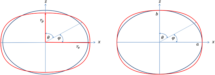
Figure 1. Meridional cross-section of the PN-ellipsoid (a red curve in on-line version) vs. the Maclaurin ellipsoid (a blue curve in on-line version). The left panel represents the most general case with arbitrary values of the shape parameters ${B}$₁, ${B}$₂, ${B}$₃ when the equatorial, r_e, and polar, r_p, radii of the PN-ellipsoid differ from the semi-major, a, and semi-minor, b, axes of the Maclaurin ellipsoid, r_e ≠ a, r_p ≠ b. The right panel shows the most important physical case of ${B}$₁ = ${B}$₂ = 0 when the equatorial and polar radii of the PN-ellipsoid and the Maclaurin ellipsoid are equal. The angle φ is the geographic latitude (−90° ≤ φ ≤ 90°), and the angle θ is a complementary angle (co-latitude) used for calculation of integrals in appendix of the present paper (0 ≤ θ ≤ π). In general, when ${B}$₁ ≠ ${B}$₂ ≠ 0, the maximal radial difference (the “height” difference) between the surfaces of the PN-ellipsoid and the Maclaurin ellipsoid depends on the choice of the post-Newtonian coordinates, and may amount to a few cm (see Section 13). Carefully operating with the residual gauge freedom of the post-Newtonian theory allows us to make the difference between the two surfaces much less than that.

Theoretical formalism for calculation of the post-Newtonian level surface can be worked out in arbitrary coordinates. For mathematical and historic reasons the most convenient are harmonic coordinates which are also used by the IAU (Soffel et al., 2003) and IERS (Petit and Luzum, 2010). The class of the harmonic coordinates is selected by the gauge condition Equation (1). Different harmonic coordinates are interrelated by coordinate transformations which are not violating the gauge condition 1. This freedom is known as a residual gauge (or coordinate) freedom. The field Equations (5)–(7) and their solutions are form-invariant with respect to the residual gauge transformations.

The residual gauge freedom is described by a post-Newtonian coordinate transformation,

$\begin{array}{ll}{x{}^{\prime }}^{\alpha }=x^{\alpha }+\kappa {\xi }^{\alpha }(x),& (28)\end{array}$

where functions, ξ^α, obey the Laplace equation,

$\begin{array}{ll}\Delta {\xi }^{\alpha }=0.& (29)\end{array}$

Solution of the Laplace equation which is convergent at the origin of the coordinate system, is given in terms of the harmonic polynomials which are selected by the conditions imposed by the statement of the problem. In our case, the problem is to determine the shape of the PN-ellipsoid which has the surface described by the polynomial of the fourth order Equation (32) with yet unknown coefficients ${B}$₁, ${B}$₂, ${B}$₃. The form of the Equation 32 does not change (in the post-Newtonian approximation) if the functions ξ^α in Equation (28) are polynomials of the third order. It is straightforward to show that the admissible harmonic polynomials of the third order have the following form

$\begin{array}{rc}{\xi }^1=hx+p\frac{x}{a^2}\left({\sigma }^2-4z^2\right),& (30\text{a})\end{array}$

$\begin{array}{rc}{\xi }^2=hy+p\frac{y}{a^2}\left({\sigma }^2-4z^2\right),& (30\text{b})\end{array}$

$\begin{array}{rc}{\xi }^3=kz+q\frac{z}{b^2}\left(3{\sigma }^2-2z^2\right),& (30\text{c})\end{array}$

where h, k, p, and q are arbitrary constant parameters. Polynomials Equations (30a)–(30c) represent solutions of the Laplace Equation (29). We choose ξ⁰ = 0 because we consider stationary spacetime so all functions are time-independent.

Coordinate transformation Equation (28) with ξⁱ taken from Equations (30a)–(30c) does not violate the harmonic gauge condition Equation (1) but it changes the numerical post-Newtonian coefficients in the mathematical form of Equations (22) and Equation (23)

$\begin{array}{r}{{K}}_1\to {{K}}_1+2h,(31\text{a})\end{array}$

$\begin{array}{r}{{K}}_2\to {{K}}_2+2k,(31\text{b})\end{array}$

$\begin{array}{r}{{B}}_1\to {{B}}_1+2p,(31\text{c})\end{array}$

$\begin{array}{r}{{B}}_2\to {{B}}_2-4q,(31\text{d})\end{array}$

$\begin{array}{r}{{B}}_3\to {{B}}_3-8p\frac{b^2}{a^2}+6q\frac{a^2}{b^2},(31\text{e})\end{array}$

Thus, it makes evident that only one out of the five coefficients ${K}$₁, ${K}$₂, ${B}$₁, ${B}$₂, ${B}$₃ is algebraically independent while the four others can be chosen arbitrary. To simplify our calculations and eliminate the gauge-dependent terms from mathematical equations we choose ${K}$₁ = ${K}$₂ = ${B}$₁ = ${B}$₂ = 0. The constant ${B}$₃ ≡ ${B}$ is left free. It will be fixed later on. With the accepted choice of the coordinates the polar radius r_p = b, the equatorial radius r_e = a, the eccentricity of the PN-ellipsoid ϵ = e, and function

$\begin{array}{l}F(\bar{\text{x}})\equiv {B}\frac{{\bar{\sigma }}^2{\bar{z}}^2}{a^2{b}^2}.(32)\end{array}$

Let xⁱ = {x, y, z} is any point inside the PN-ellipsoid. We introduce a quadratic polynomial

$\begin{array}{ll}C(\text{x})\equiv \frac{{\sigma }^2}{a^2}+\frac{z^2}{b^2}-1.& (33)\end{array}$

This polynomial vanishes on the boundary surface of the PN-ellipsoid in the Newtonian approximation. However, in the post-Newtonian approximation we have on the boundary the following condition

$\begin{array}{ll}C(\bar{\text{x}})=\kappa F(\bar{\text{x}}),& (34)\end{array}$

as a consequence of Equation (22). In terms of the polynomial $C(\overline{\text{x}})$ function $F(\overline{\text{x}})$ in Equation (32) can be formally recast to

$\begin{array}{ll}F(\bar{\text{x}})={B}\frac{{\bar{z}}^2}{b^2}\left[1+C(\bar{\text{x}})-\frac{{\bar{z}}^2}{b^2}\right].& (35)\end{array}$

The term being proportional to $C(\overline{\text{x}})$ can be discarded on the boundary of the PN-ellipsoid. Now we shall calculate the gravitational potentials of the rotating PN ellipsoid which enter the metric tensor Equations (2)–(4).

5. Newtonian Potential $\overline{v}$

Newtonian gravitational potential $\overline{V}$ satisfies the inhomogeneous Poisson's equation

$\begin{array}{ll}\Delta \bar{V}(\text{x})=-4\pi G\bar{\rho }(\text{x}),& (36)\end{array}$

inside the mass. Its particular solution is given by

$\begin{array}{ll}\bar{V}(\text{x})=G{\displaystyle {\int }_{{V}}}\frac{\bar{\rho }({\text{x}}^{\prime })d^3{x}^{\prime }}{|\text{x}-{\text{x}}^{\prime }|},& (37)\end{array}$

where ${V}$ is the volume occupied by the matter distribution. We shall assume that the density has an ellipsoidal distribution inside the body which differs from the homogeneous density, ρ₀, only in the post-Newtonian approximation. Moreover, we shall consider the most simple, linearized case of the ellipsoidal distribution

$\begin{array}{ll}\bar{\rho }(\text{x})={\rho }_0\left[1+\kappa {A}\left(\frac{{\sigma }^2}{a^2}+\frac{z^2}{b^2}\right)\right],& (38)\end{array}$

where ρ₀ is a constant bare density, and ${A}$ is as yet undetermined numerical constant. This assumption allows us to perform integration in Equation (37) explicitly. Inside the mass the integral Equation (37) can be calculated by making use of spherical coordinates. The procedure is as follows (Chandrasekhar, 1969).

Let us consider a point xⁱ = {x, y, z} inside the PN-ellipsoid Equation (22). It is connected to the point ${\overline{x}}^i$ on the surface of the ellipsoid by vector $R^i={\overline{x}}^i-x^i$ where Rⁱ = Rℓⁱ, $R=\sqrt{{\delta }_{ij}{R}^i{R}^j}$, and a unit vector, ℓⁱ = {sinθcosλ, sinθsinλ, cosθ}. We have

$\begin{array}{ll}{\bar{x}}^i=x^i+{\ell }^{i}R,& (39)\end{array}$

Substituting Equations (39)–(22) yields a quadratic equation

$\begin{array}{ll}A{R}^2+2BR+C=\kappa F\left(\text{x}+\ell R\right),& (40)\end{array}$

where

$\begin{array}{l}A\equiv \frac{{sin}^2\theta }{a^2}+\frac{{cos}^2\theta }{b^2},\\ B\equiv \frac{sin\theta \left(xcos\lambda +ysin\lambda \right)}{a^2}+\frac{zcos\theta }{b^2},\\ C\equiv \frac{{\sigma }^2}{a^2}+\frac{z^2}{b^2}-1.(41)\end{array}$

We solve Equation (40) by iterations by expanding $R=\widehat{R}+c^{-2}\Delta R$, where $\widehat{R}$ is either ${\widehat{R}}_{+}$ or ${\widehat{R}}_{-}$ corresponding to two solutions of the quadratic Equation (40) with the right hand side being nil. The bare solution $\widehat{R}$ is used, then, to calculate the right side of Equation (40) for performing the second iteration. We obtain

$\begin{array}{r}{R}_{\pm }=-\frac{B}{A}\pm \frac{\sqrt{B^2-AC+\kappa A{F}_{\pm }}}{A},(42)\end{array}$

where

$\begin{array}{r}{F}_{\pm }\equiv {B}{\left(\frac{z+cos\theta {\widehat{R}}_{\pm }}{b}\right)}^2-{B}{\left(\frac{z+cos\theta {\widehat{R}}_{\pm }}{b}\right)}^4,(43)\end{array}$

where the term $C(\overline{\text{x}})=A{R}^2+2BR+C$ vanishes because of Equation (40).

We make replacement of variable x′ in Equation (37) to r = x − x′, and use spherical coordinates to perform integration with respect to the radial coordinate r = |x − x′| from the point r = 0 to the point lying on the surface of the PN ellipsoid, r = R₋(θ, λ) or r = R₊(θ, λ). For the internal point, the angular integration in the remaining integral over the surface of the PN ellipsoid is performed over the solid angle 4π, and the integration with the point R₋(θ, λ) equals to that with the radial direction R₊(θ, λ). This observation makes the angular integration easier because the integral Equation (37) can be written down in the following form (Chandrasekhar, 1969)

$\begin{array}{ll}\bar{V}=\frac{1}{4}G{\rho }_0{{\displaystyle \oint }}_{S^2}\left(R_{+}^2+R_{-}^2\right)d\Omega +\kappa {A}{Ī}_1,& (44)\end{array}$

where R₊ and R₋ are defined in Equation (42), and the integral

$\begin{array}{ll}{Ī}_1=G{\rho }_0{\displaystyle {\int }_{{V}}}\frac{d^3{x}^{\prime }}{|\text{x}-{\text{x}}^{\prime }|}\left(\frac{{\sigma {}^{\prime }}^2}{a^2}+\frac{{z{}^{\prime }}^2}{b^2}\right)& (45)\end{array}$

takes into account the ellipsoidal distribution of the density. After making use of Equation (42) and expanding the integrand in Equation (44) with respect to the post-Newtonian parameter κ, the Newtonian potential takes on the following form

$\begin{array}{rc}\overline{V}=\frac{1}{2}G{\rho }_0{\displaystyle {\oint }_{S^2}\left\{\begin{array}{l}\frac{2B^2-AC}{A^2}+\frac{\kappa }{2A}[F_{+}+F_{-}\hfill \\ -\frac{B}{\sqrt{B^2-AC}}(F_{+}-F_{-})]\hfill \end{array}\right\}}d\Omega +\kappa A{\overline{I}}_1,& (46)\end{array}$

where all post-Newtonian terms of the higher order in κ have been discarded, and integration is performed over a unit sphere S² with respect to the angles λ and θ, dΩ ≡ sinθdθdλ is the element of the solid angle.

Now, we expand F_± in polynomial w.r.t. R_±,

$\begin{array}{l}{F}_{\pm }={\alpha }_0+{\alpha }_{1}cos\theta R_{\pm }+{\alpha }_2{\left(cos\theta R_{\pm }\right)}^2+{\alpha }_3{\left(cos\theta R_{\pm }\right)}^3\\ +{\alpha }_4{\left(cos\theta R_{\pm }\right)}^4,(47)\end{array}$

where the coefficients

$\begin{array}{rc}{\alpha }_0={B}\frac{z^2}{b^2}\left(1-\frac{z^2}{b^2}\right),& (48)\end{array}$

$\begin{array}{rc}{\alpha }_1=\frac{2{B}z}{b^2}\left(1-2\frac{z^2}{b^2}\right)& (49)\end{array}$

$\begin{array}{rc}{\alpha }_2=\frac{{B}}{b^2}\left(1-6\frac{z^2}{b^2}\right)& (50)\end{array}$

$\begin{array}{rc}{\alpha }_3=-\frac{4{B}z}{b^4},& (51)\end{array}$

$\begin{array}{rc}{\alpha }_4=-\frac{{B}}{b^4},& (52)\end{array}$

are the polynomials of z only. We also notice that on the surface of the PN-ellipsoid, $F(\overline{\text{x}})={\alpha }_0$, as follows from Equation (35) where we can use, $C(\overline{\text{x}})=0$, in the post-Newtonian terms.

Replacing Equations (47) in (46) transforms it to

$\begin{array}{ll}\bar{V}={\bar{V}}_{\text{N}}+\kappa {\bar{V}}_{\text{p}\text{N}}+\kappa {A}{Ī}_1,& (53)\end{array}$

where

$\begin{array}{ll}{\bar{V}}_{\text{N}}=G{\rho }_0{{\displaystyle \oint }}_{S^2}\left(\frac{B^2}{A^2}-\frac{C}{2A}\right)d\Omega & (54)\end{array}$

$\begin{array}{l}{\overline{V}}_{pN}=G_{\rho 0}{\displaystyle {\oint }_{S^2}[\frac{{\alpha }_0}{2A}-{\alpha }_1\cos \theta \frac{B}{A^2}+{\alpha }_2{\cos }^2\theta \left(\frac{2B^2}{A^3}-\frac{C}{2A^2}\right)}\\ -2{\alpha }_3{\cos }^3\theta \left(\frac{2B^3}{A^4}-\frac{BC}{A^3}\right)\\ +{\alpha }_4{\cos }^4\theta \left(\frac{8B^4}{A^5}-\frac{6B^{2}C}{A^4}+\frac{C^2}{2A^3}\right)]d\Omega ,& (55)\end{array}$

Equations (52)–(55) describe the Newtonian potential exactly both on the surface of the PN-ellipsoid and inside it. These equations cannot be extended to the external space which requires a separate integration which will be discussed somewhere else.

The integrals entering V in Equations (54), (55) are discussed in Appendix A in Supplementary Material. The integrals I₁ appears besides Equation (53) also in the post-Newtonian potentials of the gravitational field in Equation (80), and its discussion is postponed to section 7. After evaluating the integrals in the internal point and reducing similar terms, potentials V_N and V_pN take on the following form:

$\begin{array}{rc}{\bar{V}}_{\text{N}}=\pi G{\rho }_0{a}^2\left[\left(1-\frac{z^2}{b^2}\right){\gimel }_0-\left(1-3\frac{z^2}{b^2}\right){\gimel }_1-C(\text{x}){\gimel }_1\right],& (56)\end{array}$

$\begin{array}{rc}{\bar{V}}_{\text{p}\text{N}}=\pi G{\rho }_0{a}^2\left[F_1(z)+b^2{F}_2(z)C(\text{x})+b^4{F}_3(z)C^2(\text{x})\right],& (57)\end{array}$

where

$\begin{array}{l}{F}_1(z)={\alpha }_0{\gimel }_0-2{\alpha }_{1}z{\gimel }_1+\\ 2{\alpha }_2{b}^2[\left(1-\frac{z^2}{b^2}\right){\gimel }_1-\left(1-\frac{3z^2}{b^2}\right){\gimel }_2]\\ -4{\alpha }_3{b}^{2}z\left[3\left(1-\frac{z^2}{b^2}\right){\gimel }_2-\left(3-\frac{5z^2}{b^2}\right){\gimel }_3\right]+\\ 6{\alpha }_4{b}^4[{\left(1-\frac{z^2}{b^2}\right)}^2{\gimel }_2-2\left(1-6\frac{z^2}{b^2}+5\frac{z^4}{b^4}\right){\gimel }_3\\ +\left(1-10\frac{z^2}{b^2}+\frac{35}{3}\frac{z^4}{b^4}\right){\gimel }_4],(58)\end{array}$

$\begin{array}{l}{F}_2(z)={\alpha }_2({\gimel }_1-2{\gimel }_2)-4{\alpha }_{3}z(2{\gimel }_2-3{\gimel }_3)+\\ 6{\alpha }_4{b}^2[\left(1-\frac{z^2}{b^2}\right){\gimel }_2-3\left(1-\frac{3z^2}{b^2}\right){\gimel }_3\\ +2\left(1-\frac{5z^2}{b^2}\right){\gimel }_4],& (59)\end{array}$

$\begin{array}{rc}{F}_3(z)={\alpha }_4({\gimel }_2-6{\gimel }_3+6{\gimel }_4),& (60)\end{array}$

and the polynomial coefficients α₀, α₁, α₂, α₃, α₄ are given in Equations (48)–(52). It is worth noticing that V_pN obeys the Laplace equation

$\begin{array}{ll}\Delta {\bar{V}}_{\text{p}\text{N}}=0,& (61)\end{array}$

and Equation (57) represents the harmonic polynomial of the fourth order.

6. Post-newtonian Vector Potential ${\overline{v}}^i$

Vector potential Vⁱ obeys the Poisson equation

$\begin{array}{ll}\Delta {\bar{V}}^i=-4\pi G\bar{\rho }(\text{x})v^i(\text{x}),& (62)\end{array}$

which has a particular solution

$\begin{array}{ll}{\bar{V}}^i=G{\displaystyle {\int }_{{V}}}\frac{\bar{\rho }({\text{x}}^{\prime })v^i(x^{\prime })}{|\text{x}-{\text{x}}^{\prime }|}{d}^3{x}^{\prime }.& (63)\end{array}$

For a rigidly rotating configuration, vⁱ(x) = ε^ijkω^jx^k so that

$\begin{array}{ll}{\bar{V}}^i={\epsilon }^{ijk}{\omega }^j{\bar{{D}}}^k,& (64)\end{array}$

where

$\begin{array}{ll}{\overline{{D}}}^i=G{\displaystyle \int }\frac{\overline{\rho }({\text{x}}^{\prime }){x{}^{\prime }}^i{d}^3{x}^{\prime }}{|\text{x}-{\text{x}}^{\prime }|}.& (65)\end{array}$

It can be recast to the following form

$\begin{array}{ll}{{D}}^i=x^i{\overline{V}}_{\text{N}}+G{\displaystyle \int }\frac{\overline{\rho }({\text{x}}^{\prime })({x{}^{\prime }}^i-x^i)}{|\text{x}-{\text{x}}^{\prime }|}{d}^3{x}^{\prime },& (66)\end{array}$

where ${\overline{V}}_{\text{N}}$ is the Newtonian potential given in Equation (56). Because the potential ${\overline{V}}^i$ appears only in the post-Newtonian terms we can consider the density $\overline{\rho }$ as constant, $\overline{\rho }={\rho }_0$. In this case the second term in the right hand side of Equation (66) can be integrated over the radial coordinate, yielding

$\begin{array}{rcll}{\displaystyle {\int }_{{V}}}\frac{\overline{\rho }({\text{x}}^{\prime })({x{}^{\prime }}^i-x^i)}{|\text{x}-{\text{x}}^{\prime }|}{d}^3{x}^{\prime }& =& \frac{{\rho }_0}{6}{{\displaystyle \oint }}_{S^2}\left(R_{+}^3+R_{-}^3\right)l^{i}d\Omega .& (67)\end{array}$

After making use of Equation (42) to replace R₊ and R₋, we obtain

$\begin{array}{rcll}{\displaystyle {\int }_{{V}}}\frac{\overline{\rho }({x{}^{\prime }}^i-x^i)}{|\text{x}-{\text{x}}^{\prime }|}{d}^3{x}^{\prime }& =& {\rho }_0{{\displaystyle \oint }}_{S^2}\left(-\frac{4}{3}\frac{B^3}{A^3}+\frac{BC}{A^2}\right)l^{i}d\Omega ,& (68)\end{array}$

where we have omitted the post-Newtonian terms (with κ) since the vector potential ${\overline{V}}^i$ itself appears only in the post-Newtonian terms. Integrals entering Equation (68) are given in Appendix A in Supplementary Material. Calculation reveals

$\begin{array}{l}{\displaystyle {\int }_V\frac{\overline{\rho }(x^{\prime })(x^{\prime }-x)}{|x-x^{\prime }|}}{d}^3{x}^{\prime }=-\pi {\rho }_0{a}^{2}x[\left(1-\frac{z^2}{b^2}\right){\gimel }_0\\ -2\left(1-\frac{3z^2}{b^2}\right){\gimel }_1+\left(1-\frac{5z^2}{b^2}\right){\gimel }_2]\\ +x\pi {\rho }_0{a}^{2}C(x)({\gimel }_1-{\gimel }_2),& (69)\end{array}$

$\begin{array}{l}{\displaystyle {\int }_V\frac{\overline{\rho }(x^{\prime })(y^{\prime }-y)}{|x-x^{\prime }|}}{d}^3{x}^{\prime }=-\pi {\rho }_0{a}^{2}y[\left(1-\frac{z^2}{b^2}\right){\gimel }_0\\ -2\left(1-\frac{3z^2}{b^2}\right){\gimel }_1+\left(1-\frac{5z^2}{b^2}\right){\gimel }_2]\\ +y\pi {\rho }_0{a}^{2}C(x)({\gimel }_1-{\gimel }_2),(70)\end{array}$

$\begin{array}{l}{\displaystyle {\int }_V\frac{\overline{\rho }(x^{\prime })(z^{\prime }-z)}{|x-x^{\prime }|}}{d}^3{x}^{\prime }=-4\pi {\rho }_0{a}^{2}z[\left(1-\frac{z^2}{b^2}\right){\gimel }_1\\ -\left(1-\frac{5z^2}{3b^2}\right){\gimel }_2]-2z\pi {\rho }_0{a}^{2}C(x)({\gimel }_1-2{\gimel }_2).(71)\end{array}$

Substituting this result to Equation (66) and making use of Equation (56) yields

$\begin{array}{l}{\overline{{D}}}^i\equiv \left({\overline{{D}}}^x,{\overline{{D}}}^y,{\overline{{D}}}^z\right)=\left(x{\overline{D}}_1,y{\overline{D}}_1,z{\overline{D}}_2\right),(72)\end{array}$

where

$\begin{array}{l}{\overline{D}}_1\equiv \pi G{\rho }_0{a}^2\left[\left(1-\frac{3z^2}{b^2}\right){\gimel }_1-\left(1-\frac{5z^2}{b^2}\right){\gimel }_2-C(\text{x}){\gimel }_2\right],(73)\end{array}$

$\begin{array}{l}{\overline{D}}_2\equiv \pi G{\rho }_0{a}^2[\left(1-\frac{z^2}{b^2}\right){\gimel }_0-\left(5-7\frac{z^2}{b^2}\right){\gimel }_1+4\left(1-\frac{5z^2}{3b^2}\right){\gimel }_2\\ +C(x)(4{\gimel }_2-3{\gimel }_1)],(74)\end{array}$

7. Post-Newtonian Scalar Potential $\overline{\Phi }$

Potential $\overline{\Phi }$ is defined by equation

$\begin{array}{l}\Delta \overline{\Phi }=-4\pi G\overline{\rho }({\text{x}}^{\prime })\overline{\varphi }({\text{x}}^{\prime }),(75)\end{array}$

where function

$\begin{array}{l}\overline{\varphi }({\text{x}}^{\prime })\equiv 2{\omega }^2{\sigma }^2+3\frac{\overline{p}}{\overline{\rho }}+2{\overline{V}}_{\text{N}}.(76)\end{array}$

Potential $\overline{\Phi }$ enters only the post-Newtonian equations. Therefore, everywhere in calculation of $\overline{\Phi }$ we can assume the density $\overline{\rho }$ being approximated as constant. The pressure $\overline{p}$ inside the massive body can be calculated from the hydrostatic equilibrium equation with a constant value of the bare density $\overline{\rho }={\rho }_0$. The solution is Chandrasekhar (1969)

$\begin{array}{l}\frac{\overline{p}}{{\rho }_0}=-\pi G{\rho }_0{a}^{2}C(\text{x})\left({\gimel }_0-2{\gimel }_1\right).(77)\end{array}$

Making use of Equation (77) and Equation (56) we can write down function $\overline{\varphi }({\text{x}}^{\prime })$ as

$\begin{array}{l}\overline{\varphi }(x^{\prime })=a^2\left[2{\omega }^2-\pi G{\rho }_0(3{\gimel }_0-4{\gimel }_1)\right]\left(\frac{{\sigma }^2}{a^2}+\frac{z^2}{b^2}\right)\\ -2a^2\left[{\omega }^2-\pi G{\rho }_0({\gimel }_0-3{\gimel }_1)\right]\frac{z^2}{b^2}+\pi G{\rho }_0{a}^2(5{\gimel }_0-6{\gimel }_1).(78)\end{array}$

Particular solution of Equation (75) can be written as

$\begin{array}{l}\overline{Ф}=2{\omega }^2{a}^2\left({\overline{I}}_1-{\overline{I}}_2\right)-\pi G{\rho }_0{a}^2[\left(3{\overline{I}}_1+2{\overline{I}}_2-5{\overline{V}}_N\right){\gimel }_0\\ +2(2{\overline{I}}_1+3{\overline{I}}_2-3{\overline{V}}_N){\gimel }_1],(79)\end{array}$

where we have introduced two integrals

$\begin{array}{l}{Ī}_1=G{\rho }_0{\displaystyle {\int }_{{V}}}\frac{d^3{x}^{\prime }}{|\text{x}-{\text{x}}^{\prime }|}\left(\frac{{\sigma {}^{\prime }}^2}{a^2}+\frac{{z{}^{\prime }}^2}{b^2}\right),(80)\end{array}$

$\begin{array}{l}{Ī}_2=\frac{G{\rho }_0}{b^2}{\displaystyle {\int }_{{V}}}\frac{{z{}^{\prime }}^2}{|\text{x}-{\text{x}}^{\prime }|}{d}^3{x}^{\prime }.(81)\end{array}$

Notice that the integral Ī₁ has already appeared in the calculation of the Newtonian potential in Equation (45) while the integral Ī₂ is a new one.

The integrals can be split in several algebraic pieces,

$\begin{array}{cc}\begin{array}{l}{\overline{I}}_1=\left(\frac{{\sigma }^2}{a^2}+\frac{z^2}{b^2}\right)\left(2{\overline{D}}_1-{\overline{V}}_{\text{N}}\right)+2\frac{z^2}{b^2}\left({\overline{D}}_2-{\overline{D}}_1\right)\\ +\frac{G{\rho }_0}{8}{\displaystyle {\oint }_{S^2}(R_{+}^4+R_{-}^4)}\left(\frac{{\sin }^2\theta }{a^2}+\frac{{\cos }^2\theta }{b^2}\right)d\Omega ,\end{array}& \left(82\right)\end{array}$

$\begin{array}{cc}{\overline{I}}_2=\frac{z^2}{b^2}(2{\overline{D}}_2-{\overline{V}}_{\text{N}})+\frac{G{\rho }_0}{8b^2}{\displaystyle {\oint }_{S^2}(R_{+}^4+R_{-}^4)}{\cos }^2\theta d\Omega ,& \left(83\right)\end{array}$

where the integrals

$\begin{array}{cc}\begin{array}{l}\frac{1}{8}{\displaystyle {\oint }_{S^2}(R_{+}^4+R_{-}^4)}\left(\frac{{\sin }^2\theta }{a^2}+\frac{{\cos }^2\theta }{b^2}\right)d\Omega \\ ={\displaystyle {\oint }_{S^2}\left(\frac{2B^4}{A^3}-2\frac{B^{2}C}{A^2}+\frac{C^2}{4A}\right)}d\Omega ,\end{array}& \left(84\right)\end{array}$

$\begin{array}{ll}\begin{array}{l}\frac{1}{8}{\displaystyle {\oint }_{S^2}(R_{+}^4+R_{-}^4)}{\cos }^2\theta d\Omega \\ ={\displaystyle {\oint }_{S^2}\left(\frac{2B^4}{A^4}-2\frac{B^{2}C}{A^3}+\frac{C^2}{4A^2}\right)}{\cos }^2\theta d\Omega ,\end{array}& \left(85\right)\end{array}$

We use the results of Appendix A in Supplementary Material to calculate these integrals, and obtain

$\begin{array}{ll}\begin{array}{l}{\displaystyle {\oint }_{S^2}\left(\frac{2B^4}{A^3}-2\frac{B^{2}C}{A^2}+\frac{C^2}{4A}\right)d\Omega }\\ =\frac{3}{2}\pi a^2[{\left(1-\frac{z^2}{b^2}\right)}^2{\gimel }_0-2\left(1-6\frac{z^2}{b^2}+5\frac{z^4}{b^4}\right){\gimel }_1\\ +\left(1-10\frac{z^2}{b^2}+\frac{35}{3}\frac{z^4}{b^4}\right){\gimel }_2]+\pi a^2[\left(1-\frac{z^2}{b^2}\right){\gimel }_0\\ -4\left(1-3\frac{z^2}{b^2}\right){\gimel }_1+3\left(1-5\frac{z^2}{b^2}\right){\gimel }_2]C(x)\\ -\pi a^2\left[{\gimel }_1-\frac{3}{2}{\gimel }_2\right]C^2(x)\end{array}& \left(86\right)\end{array}$

$\begin{array}{cc}\begin{array}{l}{\displaystyle {\oint }_{S^2}\left(\frac{2B^4}{A^4}-2\frac{B^{2}C}{A^3}+\frac{C^2}{4A^2}\right)\frac{{\cos }^2\theta }{b^2}d\Omega }\\ =\frac{3}{2}\pi a^2[{\left(1-\frac{z^2}{b^2}\right)}^2{\gimel }_1-2\left(1-6\frac{z^2}{b^2}+5\frac{z^4}{b^4}\right){\gimel }_2\\ +\left(1-10\frac{z^2}{b^2}+\frac{35}{3}\frac{z^4}{b^4}\right){\gimel }_3]\\ +\pi a^2\left(1-\frac{z^2}{b^2}\right){\gimel }_1-4\left(1-3\frac{z^2}{b^2}\right){\gimel }_2\\ +3\left(1-5\frac{z^2}{b^2}\right){\gimel }_3]C(x)+\pi a^2\left[{\gimel }_2-\frac{3}{2}{\gimel }_3\right]C^2(x)\end{array}& \left(87\right)\end{array}$

Substituting these results in Equations (82) and (83) yields

$\begin{array}{cc}\begin{array}{l}{\overline{I}}_1=\frac{1}{2}\pi G{\rho }_0{a}^2[\left(1-\frac{z^4}{b^4}\right){\gimel }_0-6\frac{z^2}{b^2}\left(1-\frac{5}{3}\frac{z^2}{b^2}\right){\gimel }_1\\ -\left(1-10\frac{z^2}{b^2}+\frac{35}{3}\frac{z^4}{b^4}\right){\gimel }_2]\\ -\pi G{\rho }_0{a}^2\left[\frac{3z^2}{b^2}{\gimel }_1+\left(1-5\frac{z^2}{b^2}\right){\gimel }_2+\frac{1}{2}{\gimel }_{2}C(x)\right]C(x),\end{array}& \left(88\right)\end{array}$

$\begin{array}{cc}\begin{array}{l}{\overline{I}}_2=\pi G{\rho }_0{a}^2[\left(1-\frac{z^2}{b^2}\right)\frac{z^2}{b^2}{\gimel }_0+\left(\frac{3}{2}-12\frac{z^2}{b^2}+\frac{25}{2}\frac{z^4}{b^4}\right){\gimel }_1\\ -\left(3-26\frac{z^2}{b^2}+\frac{85}{3}\frac{z^4}{b^4}\right){\gimel }_2+\left(\frac{3}{2}-15\frac{z^2}{b^2}+\frac{35}{2}\frac{z^4}{b^4}\right){\gimel }_3]\\ +\pi G\rho a^2[\left(1-6\frac{z^2}{b^2}\right){\gimel }_1-4\left(1-5\frac{z^2}{b^2}\right){\gimel }_2\\ +3\left(1-5\frac{z^2}{b^2}\right){\gimel }_3+\left({\gimel }_2-\frac{3}{2}{\gimel }_3\right)\text{C(}x\text{)}]\text{C(}x\text{)}\text{.}\end{array}& \left(89\right)\end{array}$

Replacing these expressions to Equation (79) results in

$\begin{array}{cc}\overline{\Phi }={\Phi }_0+{\Phi }_{1}C(x)+{\Phi }_2{C}^2(x),& \left(90\right)\end{array}$

where

$\begin{array}{cc}\begin{array}{l}{\Phi }_0=\frac{1}{2}{\pi }^2{G}^2{\rho }_0^2{a}^4[7{\gimel }_0^2-3{\gimel }_0(8{\gimel }_1-5{\gimel }_2+2{\gimel }_3)\\ +2{\gimel }_1(15{\gimel }_1-20{\gimel }_2+9{\gimel }_3)]-{\pi }^2{G}^2{\rho }_0^2{a}^4[7{\gimel }_0^2\\ +{\gimel }_0(-60{\gimel }_1+67{\gimel }_2-30{\gimel }_3)+2{\gimel }_1(51{\gimel }_1-88{\gimel }_2\\ +45{\gimel }_3)]\frac{z^2}{b^2}+\frac{1}{6}{\pi }^2{G}^2{\rho }_0^2{a}^4[21{\gimel }_0^2+{\gimel }_0(-288{\gimel }_1+445{\gimel }_2\\ -210{\gimel }_3)+10{\gimel }_1(57{\gimel }_1-116{\gimel }_2+63{\gimel }_3)]\frac{z^4}{b^4}\\ +\pi G{\rho }_0{a}^4{\omega }^2[{\gimel }_0-3{\gimel }_1+5{\gimel }_2-3{\gimel }_3-2({\gimel }_0-9{\gimel }_1+21{\gimel }_2\\ -15{\gimel }_3)\frac{z^2}{b^2}+({\gimel }_0-5(3{\gimel }_1-9{\gimel }_2+7{\gimel }_3))\frac{z^4}{b^4}],\end{array}& \left(91\right)\end{array}$

$\begin{array}{cc}\begin{array}{l}{\Phi }_1={\pi }^2{G}^2{\rho }_0^2{a}^4[{\gimel }_0(-7{\gimel }_1+11{\gimel }_2-6{\gimel }_3)+2{\gimel }_1(6{\gimel }_1\\ -14{\gimel }_2+9{\gimel }_3)]+{\pi }^2{G}^2{\rho }_0^2{a}^4[{\gimel }_0(21{\gimel }_1-55{\gimel }_2+30{\gimel }_3)\\ -2{\gimel }_1(24{\gimel }_1-70{\gimel }_2+45{\gimel }_3)]\frac{z^2}{b^2}-2\pi G{\rho }_0{a}^4{\omega }^2[({\gimel }_1\\ -3{\gimel }_2+3{\gimel }_3)-3({\gimel }_1-5{\gimel }_2+5{\gimel }_3)\frac{z^2}{b^2}]\end{array}& \left(92\right)\end{array}$

$\begin{array}{l}{\Phi }_2=\frac{1}{2}\pi G{\rho }_0{a}^4[(-{\gimel }_0{\gimel }_2+8{\gimel }_1{\gimel }_2+6{\gimel }_0{\gimel }_3-18{\gimel }_1{\gimel }_3)\pi G{\rho }_0\\ -6({\gimel }_2-{\gimel }_3){\omega }^2],& \left(93\right)\hfill \end{array}$

This finalizes the calculation of the post-Newtonian potentials inside the mass.

8. Post-Newtonian Mass

The post-Newtonian conservation laws have been discussed by a number of researchers the most notably in textbooks (Fock, 1964; Will, 1993; Kopeikin et al., 2011). General relativity predicts that the integrals of energy, linear momentum, angular momentum and the center of mass of an isolated system are conserved in the post-Newtonian approximation. In the present paper we deal with a single isolated body so that the integrals of the center of mass and the linear momentum are trivial and we can always choose the origin of the coordinate system at the center of mass of the body with the linear momentum being nil. The integrals of energy and angular momentum are less trivial and requires detailed calculations which are given below.

The law of conservation of energy yields the post-Newtonian mass of a rotating fluid ball that is defined as follows (Fock, 1964; Will, 1993; Kopeikin et al., 2011)

$\begin{array}{ll}M=M_{\text{N}}+\frac{1}{c^2}{M}_{\text{p}\text{N}},& \left(94\right)\hfill \end{array}$

where ${V}$ is the volume of PN-ellipsoid, and

$\begin{array}{ll}{M}_{\text{N}}={\displaystyle {\int }_{{V}}}\overline{\rho }(\text{x})d^{3}x,& \left(95\right)\hfill \end{array}$

is the rest mass of baryons comprising the body, and

$\begin{array}{ll}{M}_{\text{p}\text{N}}={\displaystyle {\int }_{{V}}}\overline{\rho }(\text{x})\left(v^2+\Pi +\frac{5}{2}{V}_{\text{N}}\right)d^{3}x,& \left(96\right)\hfill \end{array}$

is the post-Newtonian correction.

In order to calculate the rest mass, M_N, we introduce normalized spherical coordinates r, θ, ϕ related to the Cartesian (harmonic) coordinates x, y, z as follows,

$\begin{array}{ll}x=arsin\theta cos\varphi ,y=arsin\theta sin\varphi ,z=brcos\theta .& \left(97\right)\hfill \end{array}$

In these coordinates the integral Equation (95) is given by

$\begin{array}{ll}{M}_{\text{N}}=a^{2}b{\rho }_0{\displaystyle \underset{0}{\overset{r(\theta )}{\int }}}{\displaystyle \underset{0}{\overset{\pi }{\int }}}{\displaystyle \underset{0}{\overset{2\pi }{\int }}}\left(1+\kappa {A}{r}^2\right)r^{2}sin\theta drd\theta d\varphi ,& \left(98\right)\hfill \end{array}$

where r(θ) describes the surface of the PN-ellipsoid defined above in Equations (22), (32)

$\begin{array}{ll}{r}^2(\theta )=1+\kappa {B}{sin}^2{cos}^2\theta .& \left(99\right)\hfill \end{array}$

Integration in Equation (98) results in

$\begin{array}{ll}{M}_{\text{N}}=\frac{4\pi }{3}{\rho }_0{a}^{2}b\left[1+\frac{\kappa }{5}\left({A}+{B}\right)\right].& \left(100\right)\hfill \end{array}$

The post-Newtonian contribution, M_pN, to the rest mass reads

$\begin{array}{l}{M}_{\text{pN}}={\rho }_0{a}^{4}b{\displaystyle \underset{0}{\overset{1}{\int }}{\displaystyle \underset{0}{\overset{\pi }{\int }}{\displaystyle \underset{0}{\overset{2\pi }{\int }}}}}\{{\omega }^2{r}^2{\sin }^2\theta +\frac{5}{2}\pi G{\rho }_0[{\gimel }_0(1-r^2{\cos }^2\theta )\\ -{\gimel }_1{r}^2(1-3{\cos }^2\theta )]\}{r}^2\sin \theta drd\theta d\varphi \\ =\frac{8\pi }{15}{\rho }_0{a}^{4}b({\omega }^2+5\pi G{\rho }_0{\gimel }_0).& \left(101\right)\hfill \end{array}$

The total mass Equation (94) becomes

$\begin{array}{ll}M=\frac{4\pi }{3}{\rho }_0{a}^{2}b\left[1+\frac{\kappa }{5}\left(\frac{2{\omega }^2}{\pi G{\rho }_0}+{A}+{B}+10{\gimel }_0\right)\right].& \left(102\right)\hfill \end{array}$

The inverse relation is used to convert the density ρ₀ to the total mass,

$\begin{array}{ll}{\rho }_0=\frac{3M}{4\pi a^{2}b}\left[1-\frac{\kappa }{5}\left({A}+{B}+10{\gimel }_0+\frac{2{\omega }^2}{\pi G{\rho }_0}\right)\right].& \left(103\right)\hfill \end{array}$

The total post-Newtonian mass, M, depends on the sum of the parameters, ${A}$+${B}$.

9. Post-Newtonian Angular Momentum

Vector of the post-Newtonian angular momentum, Sⁱ = (S^x, S^y, S^z), is defined by Fock (1964), Will (1993), and Kopeikin et al. (2011)

$\begin{array}{l}{S}^i=S_{\text{N}}^i+\frac{1}{c^2}{S}_{\text{p}\text{N}}^i,(104)\end{array}$

where $S_{\text{N}}^i$ and $S_{\text{pN}}^i$ are the Newtonian and post-Newtonian contributions respectively,

$\begin{array}{l}{S}_{\text{N}}^i=\int \overline{\rho }(\text{x}){\left(\text{x}\times \text{v}\right)}^i{d}^{3}x,(105)\end{array}$

$\begin{array}{r}\begin{array}{l}{S}_{pN}^i={{\displaystyle \int }}^{\text{}}\overline{\rho }(x)\left(v^2+6\overline{V}+\frac{\overline{p}}{\overline{\rho }}\right){\left(x\times v\right)}^i{d}^{3}x\hfill \\ -4{{\displaystyle \int }}^{\text{}}\overline{\rho }(x){\left(x\times \overline{V}\right)}^i{d}^{3}x,\hfill \end{array}(106)\end{array}$

and vector-potential $\overline{\text{V}}\equiv {\overline{V}}^i$ has been given in Equations (64) and (72).

It can be checked up by inspection that in case of an axisymmetric mass distribution with the ellipsoidal density distribution Equation (38), the only non-vanishing component of the angular momentum is S³ = S^z ≡ S. Indeed, v = (ω × x), and (x × v)ⁱ = (x × (ω × x))ⁱ = ωⁱ(x² + y² + z²) − xⁱ ω z. It results in

$\begin{array}{l}{S}_{\text{N}}^x=-\omega {\displaystyle \int \overline{\rho }}xz{d}^{3}x,S_{\text{N}}^y=-\omega {\displaystyle \int \overline{\rho }}yz{d}^{3}x,\\ S_{\text{N}}^z=\omega {\displaystyle \int \overline{\rho }}(x^2+y^2)d^{3}x.(107)\end{array}$

By making use of the coordinates Equation (97) the reader can easily confirm that $S_{\text{N}}^x=S_{\text{N}}^y=0$, and $S_{\text{N}}^z\equiv S_{\text{N}}$ reads

$\begin{array}{l}{S}_{\text{N}}=a^{4}b\omega {\displaystyle \underset{0}{\overset{r(\theta )}{\int }}}{\displaystyle \underset{0}{\overset{\pi }{\int }}}{\displaystyle \underset{0}{\overset{2\pi }{\int }}}\overline{\rho }(\text{x})r^4{sin}^3\theta drd\theta d\varphi ,(108)\end{array}$

where r(θ) is defined in Equation (99). After integration we obtain,

$\begin{array}{l}{S}_{\text{N}}=\frac{8\pi }{15}{a}^{4}b{\rho }_0\omega \left[1+\frac{\kappa }{7}\left(5{A}+2{B}\right)\right].(109)\end{array}$

Replacing the density ρ₀ by the total mass M with the help of Equation (102), makes the Newtonian part of the angular momentum take on the following form,

$\begin{array}{l}{S}_{\text{N}}=\frac{2}{5}M{a}^2\omega \left[1-\frac{\kappa }{35}\left(2{A}-3{B}+70{\gimel }_0+\frac{14{\omega }^2}{\pi G{\rho }_0}\right)\right].(110)\end{array}$

It is straightforward to prove that x and y components of $S_{\text{pN}}^i$ also vanish due to the axial symmetry, and only its z component, $S_{\text{pN}}^z\equiv S_{\text{pN}}$, remains. We notice that

$\begin{array}{l}\int \overline{\rho }(\text{x}){\left(\text{x}\times \overline{\text{V}}\right)}^z{d}^{3}x=\int \overline{\rho }(\text{x}){\overline{D}}_1{\left(\text{x}\times \text{v}\right)}^z{d}^{3}x,(111)\end{array}$

where D₁ is taken from Equation (73). Therefore,

$\begin{array}{l}{S}_{\text{p}\text{N}}=\int \overline{\rho }(\text{x})\left(v^2+6{\overline{V}}_{\text{N}}+\frac{\overline{p}}{\overline{\rho }}-4{\overline{D}}_1\right){\left(\text{x}\times \text{v}\right)}^z{d}^{3}x.(112)\end{array}$

Making transformation to the coordinates Equation (97) and approximating $\overline{\rho }={\rho }_0$, yields

$\begin{array}{l}{S}_{\text{pN}}=\omega a^{6}b{\rho }_0{\displaystyle \underset{0}{\overset{1}{\int }}{\displaystyle \underset{0}{\overset{\pi }{\int }}{\displaystyle \underset{0}{\overset{2\pi }{\int }}\{}}}{\omega }^2{r}^2{\sin }^2\theta +7{\gimel }_0-6{\gimel }_1-({\gimel }_0+4{\gimel }_1\\ -4{\gimel }_2)r^2-2(3{\gimel }_0-15{\gimel }_1+10{\gimel }_2)r^2{\cos }^2\theta \}\\ r^4{\sin }^3\theta drd\theta d\varphi \\ =\frac{4}{35}M{a}^2\omega [2{\omega }^2+\pi G{\rho }_0(19{\gimel }_0-16{\gimel }_1)].(113)\end{array}$

The total angular momentum becomes

$\begin{array}{l}S=\frac{2}{5}M{a}^2\omega \left\{1-\frac{\kappa }{35}\left[2{A}-3{B}-40\left(3{\gimel }_0-4{\gimel }_1\right)-\frac{6{\omega }^2}{\pi G{\rho }_0}\right]\right\}.(114)\end{array}$

10. Post-Newtonian Equation of the Level Surface

The figure of the rotating fluid body is defined by the boundary condition of vanishing pressure, p = 0. The surface p = 0 is called the level surface. Relativistic Euler equation derived for the rigidly rotating fluid body tells us that the level surface coincides with the equipotential surface of the post-Newtonian gravitational potential $\overline{W}$ which is expressed in terms of the centrifugal and gravitational potentials by the following expression (Kopejkin, 1991; Kopeikin et al., 2011, 2015)

$\begin{array}{r}\begin{array}{l}\begin{array}{l}\overline{W}=\frac{1}{2}{\omega }^2{\sigma }^2+{\overline{V}}_N+\kappa ({\overline{V}}_{pN}+A{\overline{I}}_1)+\frac{1}{c^2}(\frac{1}{8}{\omega }^4{\sigma }^4\\ +\frac{3}{2}{\omega }^2{\sigma }^2{\overline{V}}_N-4{\omega }^2{\sigma }^2{\overline{D}}_1-\frac{1}{2}{\overline{V}}_N^2+\overline{\Phi }),\end{array}\hfill \\ \hfill \end{array}(115)\end{array}$

where $\kappa \equiv \pi G{\rho }_0{a}^2∕c^2$, and the potentials ${\overline{V}}_{\text{N}},{\overline{V}}_{\text{pN}},{Ī}_1,{\overline{D}}_1,\overline{\Phi }$ have been explained in Sections 5–7. After substituting these potentials to equation Equation (115) it can be presented as a quadratic polynomial with respect to function C(x),

$\begin{array}{l}\overline{W}(\text{x})={\overline{W}}_0+{\overline{W}}_{1}C(\text{x})+{\overline{W}}_2{C}^2(\text{x}),(116)\end{array}$

where the coefficients of the expansion are the polynomials of the z coordinate only. In particular, the coefficient ${\overline{W}}_0$ is a polynomial of the fourth order,

$\begin{array}{l}{\overline{W}}_0=K_0+K_1\frac{z^2}{b^2}+K_2\frac{z^4}{b^4},(117)\end{array}$

where

$\begin{array}{l}{K}_0=\frac{1}{2}{\omega }^2{a}^2+\pi G{\rho }_0{a}^2({\gimel }_0-{\gimel }_1)\hfill \\ +\frac{1}{8c^2}{\omega }^4{a}^4+\frac{1}{2}\kappa {\omega }^2{a}^2(5{\gimel }_0-17{\gimel }_1+18{\gimel }_2-6{\gimel }_3)\hfill \\ +\frac{1}{2}\kappa \pi G{\rho }_0{a}^2[6{\gimel }_0^2-{\gimel }_0(22{\gimel }_1-15{\gimel }_2+6{\gimel }_3)\hfill \\ +{\gimel }_1(29{\gimel }_1-40{\gimel }_2+18{\gimel }_3)]+\kappa \pi G{\rho }_0{a}^2[2({\gimel }_1-4{\gimel }_2\hfill \\ +6{\gimel }_3-3{\gimel }_4){B}+\frac{1}{2}({\gimel }_0-{\gimel }_2){A}],(118)\hfill \end{array}$

$\begin{array}{l}{K}_1=-\frac{1}{2}{\omega }^2{a}^2-\pi G{\rho }_0{a}^2({\gimel }_0-3{\gimel }_1)\\ -\frac{1}{4c^2}{\omega }^4{a}^4-\kappa {\omega }^2{a}^2(5{\gimel }_0-40{\gimel }_1+66{\gimel }_2-30{\gimel }_3)\\ -\kappa \pi G{\rho }_0{a}^2(6{\gimel }_0^2-56{\gimel }_0{\gimel }_1+99{\gimel }_1^2+67{\gimel }_0{\gimel }_2-176{\gimel }_1{\gimel }_2\\ -30{\gimel }_0{\gimel }_3+90{\gimel }_1{\gimel }_3)+\kappa \pi G{\rho }_0{a}^2[({\gimel }_0-18{\gimel }_1+78{\gimel }_2\\ -120{\gimel }_3+60{\gimel }_4)B-(3{\gimel }_1-5{\gimel }_2)A],(119)\end{array}$

$\begin{array}{l}{K}_2=\frac{1}{8c^2}{\omega }^4{a}^4+\frac{1}{2}\kappa {\omega }^2{a}^2(5{\gimel }_0-63{\gimel }_1+130{\gimel }_2-70{\gimel }_3)\hfill \\ +\frac{1}{6}\kappa \pi G{\rho }_0{a}^2[18{\gimel }_0^2-5{\gimel }_0(54{\gimel }_1-89{\gimel }_2\hfill \\ +42{\gimel }_3)+{\gimel }_1(543{\gimel }_1-1160{\gimel }_2+630{\gimel }_3)]\hfill \\ -\kappa \pi G{\rho }_0{a}^2[({\gimel }_0-20{\gimel }_1+90{\gimel }_2-140{\gimel }_3+70{\gimel }_4){B}\hfill \\ +\frac{1}{2}\left({\gimel }_0-10{\gimel }_1+\frac{35}{3}{\gimel }_2\right){A}].(120)\hfill \end{array}$

Coefficient ${\overline{W}}_1$ in Equation (116) is a polynomial of the second order,

$\begin{array}{l}{\overline{W}}_1=P+P_1\frac{z^2}{b^2},(121)\end{array}$

where

$\begin{array}{l}P=\frac{1}{2}{\omega }^2{a}^2\left[1+\frac{1}{2c^2}{\omega }^2{a}^2+\kappa (3{\gimel }_0-18{\gimel }_1+28{\gimel }_2-12{\gimel }_3)\right]\hfill \\ -\pi G{\rho }_0{a}^2{\gimel }_1+\kappa \pi G{\rho }_0{a}^2[({\gimel }_1-8{\gimel }_2+18{\gimel }_3-12{\gimel }_4){B}\hfill \\ -{\gimel }_2{A}]-\kappa \pi G{\rho }_0{a}^2(6{\gimel }_0{\gimel }_1-11{\gimel }_1^2-11{\gimel }_0{\gimel }_2+28{\gimel }_1{\gimel }_2\hfill \\ +6{\gimel }_0{\gimel }_3-18{\gimel }_1{\gimel }_3),(122)\hfill \end{array}$

$\begin{array}{l}{P}_1=-\frac{1}{4c^2}{\omega }^2{a}^4-\frac{3}{2}\kappa {\omega }^2{a}^2({\gimel }_0-16{\gimel }_1+36{\gimel }_2-20{\gimel }_3)\\ +\kappa \pi G{\rho }_0{a}^2[20{\gimel }_0{\gimel }_1-45{\gimel }_1^2-55{\gimel }_0{\gimel }_2+140{\gimel }_1{\gimel }_2\\ +30{\gimel }_0{\gimel }_3-90{\gimel }_1{\gimel }_3]-\kappa \pi G{\rho }_0{a}^2[2(3{\gimel }_1-25{\gimel }_2+51{\gimel }_3\\ -30{\gimel }_4)B+(3{\gimel }_1-5{\gimel }_2)A].(123)\end{array}$

Coefficient ${\overline{W}}_2$ in Equation (116) is constant,

$\begin{array}{l}{\overline{W}}_2=\frac{1}{8c^2}{\omega }^4{a}^4-\frac{1}{2}\kappa {\omega }^2{a}^2(3{\gimel }_1-2{\gimel }_2-6{\gimel }_3)\hfill \\ -\kappa \pi G{\rho }_0{a}^2[({\gimel }_2-6{\gimel }_3+6{\gimel }_4){B}+\frac{1}{2}{\gimel }_2{A}\hfill \\ +\frac{1}{2}({\gimel }_1^2+{\gimel }_0{\gimel }_2-8{\gimel }_1{\gimel }_2-6{\gimel }_0{\gimel }_3+18{\gimel }_1{\gimel }_3)].(124)\hfill \end{array}$

On the level surface of the PN-ellipsoid² we have all three coordinates interconnected by Equation (34) of the PN-ellipsoid, $C(\overline{\text{x}})=\kappa {\alpha }_0(\overline{z})$, so that Equation (116) becomes

$\begin{array}{l}\overline{W}\equiv {\overline{W}}_0+\kappa {\overline{W}}_1{\alpha }_0(\overline{z}),(125)\end{array}$

and the term with ${\overline{W}}_2~{O}({\kappa }^2)$, is discarded as negligibly small. After reducing similar terms, the potential $\overline{W}$ on the level surface is simplified to the polynomial of the fourth order,

$\begin{array}{l}\overline{W}={\overline{K}}_0+{\overline{K}}_1\frac{{\overline{z}}^2}{b^2}+{\overline{K}}_2\frac{{\overline{z}}^4}{b^4},(126)\end{array}$

where

$\begin{array}{l}{\overline{K}}_0=K_0,(127)\end{array}$

$\begin{array}{l}{\overline{K}}_1=K_1+\kappa \left(\frac{1}{2}{\omega }^2{a}^2-\pi G{\rho }_0{a}^2{\gimel }_1\right){B},(128)\end{array}$

$\begin{array}{l}{\overline{K}}_2=K_2-\kappa \left(\frac{1}{2}{\omega }^2{a}^2-\pi G{\rho }_0{a}^2{\gimel }_1\right){B}.(129)\end{array}$

Because the potential $\overline{W}$ is to be constant on the level surface (Kopeikin et al., 2015), the numerical coefficients ${\overline{K}}_1$ and ${\overline{K}}_2$ must vanish. The first condition, ${\overline{K}}_1=0$, yields a relation between the angular velocity of rotation, ω, and the eccentricity, e, of the rotating fluid ellipsoid:

$\begin{array}{l}\frac{{\omega }^2}{2\pi G{\rho }_0}[1+\frac{{\omega }^2{a}^2}{2c^2}+2\kappa (5{\gimel }_0-40{\gimel }_1+66{\gimel }_2-30{\gimel }_3-{B})]\\ =3{\gimel }_1-{\gimel }_0-\kappa [6{\gimel }_0^2-56{\gimel }_0{\gimel }_1+99{\gimel }_1^2+67{\gimel }_0{\gimel }_2-176{\gimel }_1{\gimel }_2\\ -30{\gimel }_0{\gimel }_3+90{\gimel }_1{\gimel }_3+(3{\gimel }_1-5{\gimel }_2)A-({\gimel }_0-18{\gimel }_1+78{\gimel }_2\\ -120{\gimel }_3+60{\gimel }_4){B}].(130)\end{array}$

Equation (130) generalizes the famous result that was first obtained by Colin Maclaurin in 1742, from the Newtonian theory of gravity to the realm of general relativity.

The second condition, ${\overline{K}}_2=0$, yields an algebraic equation for the two coefficients ${A}$, ${B}$,

$\begin{array}{l}\frac{1}{2}({\gimel }_0-10{\gimel }_1+\frac{35}{3}{\gimel }_2){A}+(\frac{{\omega }^2}{2\pi G{\rho }_0}+{\gimel }_0-21{\gimel }_1+90{\gimel }_2\\ -140{\gimel }_3+70{\gimel }_4){B}=\frac{{\omega }^4}{8{\pi }^2{G}^2{\rho }^2}+\frac{{\omega }^2}{4\pi G\rho }(5{\gimel }_0-63{\gimel }_1\\ +130{\gimel }_2-70{\gimel }_3)+\frac{1}{6}[18{\gimel }_0^2-5{\gimel }_0(54{\gimel }_1-89{\gimel }_2+42{\gimel }_3)\\ +{\gimel }_1(543{\gimel }_1-1160{\gimel }_2+630{\gimel }_3)].(131)\end{array}$

Equation (131) imposes one constraint on two coefficients ${A}$, ${B}$ defining the shape of the PN-ellipsoid and the law of distribution of mass density. One more constraint is required to fix these coefficients. We can use, for example, the Maclaurin relation Equation (130) to set an additional (geodetic) constraint on the parameters by demanding that the post-Newtonian part of Equation (130) vanishes.

We explored another possibility to impose self-consistent constraints on the shape parameters of the PN-ellpsoid directly related to the gravimetric measurements in geodesy. Newtonian theory of rotating reference-ellipsoid connects the shape parameters of the Maclaurin ellipsoid with the measured values of its gravity force at the pole and equator of the ellipsoid through the Pizzetti and Clairaut theorems (Pizzetti, 1913; Torge and Müller, 2012). Let us denote the force of gravity measured at the pole of the ellipsoid by γ_p ≡ γ_i(x = 0, y = 0, z = b), and the force of gravity measured on equator by γ_e ≡ γ_i(x = 0, y = a, z = 0). Due to the rotational symmetry of the ellipsoid the equatorial point can be, in fact, chosen arbitrary. The classic form of the Pizetti theorem is

$\begin{array}{l}2\frac{{\gamma }_e}{a}+\frac{{\gamma }_p}{b}=\frac{3GM}{a^{2}b}-2{\omega }^2,(132)\end{array}$

while the Clairaut theorem states

$\begin{array}{l}\frac{{\gamma }_e}{a}-\frac{{\gamma }_p}{b}=\frac{3GM}{2a^{2}b}\frac{3e-e^3-3\sqrt{1-e^2}\arcsin e}{e^3}+{\omega }^2.(133)\end{array}$

These two theorems were crucial in geodesy of XIX-th century for deeper understanding that the geometric shape of Earth's figure can be determined not only from the measurements of the geodetic arcs but, independently, from rendering the intrinsic measurements of the force of gravity on its surface. The gravity-geometry correspondence led to the pioneering idea that the gravity force and geometry of space must be always interrelated—the idea which paved a way in XX-th century to the development of the general theory of relativity by A. Einstein. We derive the post-Newtonian analogs of the Pizzetti and Clairaut theorems in the next two sections and explore what kind of natural limitations (if any) they can set on the shape parameters of the post-Newtonian ellipsoid.

11. Post-Newtonian Pizzetti's Theorem

The force of gravity on the equipotential surface of a massive rotating body is defined by equation (Kopeikin et al., 2011)

$\begin{array}{l}{\gamma }_i={[{\Lambda }^j{}_i{\partial }_j\overline{W}]}_{x=\overline{x}},(134)\end{array}$

where ${\partial }_i\equiv \partial ∕\partial x^i$, the post-Newtonian gravity potential $\overline{W}$ is given in Equation (116), and

$\begin{array}{l}{\Lambda }^j{}_i={\delta }^{ij}(1-\frac{1}{c^2}{\overline{V}}_{\text{N}})-\frac{1}{2c^2}{v}^i{v}^j,(135)\end{array}$

is the matrix of transformation from the global coordinates to the local inertial frame of observer, vⁱ = (ω × x)ⁱ is velocity of the observer with respect to the global coordinates, and V_N is the Newtonian potential Equation (56). We emphasize that we, first, take a derivative in Equation (134), and then, take the spatial coordinates, x, on the equipotential surface described by the equation of the post-Newtonian ellipsoid Equation (22).

Velocity vⁱ is orthogonal to the gradient ${\partial }_i\overline{W}$ everywhere, that is

$\begin{array}{l}{v}^i{\partial }_i\overline{W}=0.(136)\end{array}$

Indeed, it is easy to prove that

$\begin{array}{l}{v}^i{\partial }_i\overline{W}=\omega (x{\partial }_y\overline{W}-y{\partial }_x\overline{W}).(137)\end{array}$

Partial derivatives of W are calculated from Equation (116),

$\begin{array}{l}{\partial }_x\overline{W}=\frac{d\overline{W}}{dC}{\partial }_{x}C(x)=\frac{d\overline{W}}{dC}\frac{2x}{a^2},{\partial }_y\overline{W}=\frac{d\overline{W}}{dC}{\partial }_{y}C(x)=\frac{d\overline{W}}{dC}\frac{2y}{a^2}.(138)\end{array}$

Replacing the partial derivative from Equations (138) to (137) yields Equation (136). After accounting for Equations (136), (134) is simplified to

$\begin{array}{l}{\gamma }_i(\overline{x})={\left[\right(1-\frac{1}{c^2}{\overline{V}}_{\text{N}}\left){\partial }_i\overline{W}\right]}_{x=\overline{x}}.(139)\end{array}$

We shall denote the force of gravity on the pole by γ_p ≡ γ_i(x = 0, y = 0, z = r_p), and the force of gravity on the equator by γ_e ≡ γ_i(x = 0, y = r_e, z = 0) where the equatorial r_e and polar r_p radii are defined in Equations (24) and (25) respectively. Taking the partial derivative from $\overline{W}$ in Equation (139), yields

$\begin{array}{l}{\gamma }_p=\frac{2\pi G{\rho }_0{a}^2}{b}({\gimel }_0-2{\gimel }_1)+16\frac{{\omega }^2{a}^2}{b}\kappa ({\gimel }_1-3{\gimel }_2+2{\gimel }_3)\\ +\frac{2\pi G{\rho }_0{a}^2}{b}\kappa [({\gimel }_0-17{\gimel }_1+60{\gimel }_2-76{\gimel }_3+32{\gimel }_4)B\\ +({\gimel }_0-4{\gimel }_1+\frac{8}{3}{\gimel }_2)A]+\frac{4\pi G{\rho }_0{a}^2}{3b}\kappa [{\gimel }_0(27{\gimel }_1-56{\gimel }_2\\ +24{\gimel }_3)-2{\gimel }_1(33{\gimel }_1-74{\gimel }_2+36{\gimel }_3)],(140)\end{array}$

$\begin{array}{l}{\gamma }_e=a(2{\gimel }_{1}G\pi {\rho }_0\text{}-\text{}{\omega }^2)-\frac{{\omega }^4{a}^3}{2c^2}+\kappa [-3{\gimel }_0+18{\gimel }_1-28{\gimel }_2\\ +12{\gimel }_3+({\gimel }_0-{\gimel }_1)]{\omega }^{2}a-2\kappa \pi G{\rho }_{0}a[({\gimel }_1-8{\gimel }_2+18{\gimel }_3\\ -12{\gimel }_4)B+{\gimel }_{2}A]+2\kappa \pi G{\rho }_{0}a[{\gimel }_0(5{\gimel }_1-11{\gimel }_2+6{\gimel }_3)\\ -2{\gimel }_1(5{\gimel }_1-14{\gimel }_2+9{\gimel }_3)].(141)\end{array}$

We form a linear combination

$\begin{array}{l}2\frac{{\gamma }_e}{a}+\frac{{\gamma }_p}{b}=2\pi G{\rho }_0[2{\gimel }_1+\frac{a^2}{b^2}({\gimel }_0-2{\gimel }_1)]-2{\omega }^2-\frac{1}{c^2}{\omega }^4{a}^2\\ -2\kappa [2{\gimel }_0-17{\gimel }_1+28{\gimel }_2-12{\gimel }_3-8\frac{a^2}{b^2}({\gimel }_1\\ -3{\gimel }_2+2{\gimel }_3)]{\omega }^2-2\kappa \pi G{\rho }_0[2{\gimel }_1-16{\gimel }_2+36{\gimel }_3\\ -24{\gimel }_4-\frac{a^2}{b^2}({\gimel }_0-17{\gimel }_1+60{\gimel }_2-76{\gimel }_3+32{\gimel }_4)]B\\ -2\kappa \pi G{\rho }_0[2{\gimel }_2+\frac{a^2}{b^2}({\gimel }_0-4{\gimel }_1+\frac{8}{3}{\gimel }_2)]A\\ +4\kappa \pi G{\rho }_0[{\gimel }_0(5{\gimel }_1-11{\gimel }_2+6{\gimel }_3)-2{\gimel }_1(5{\gimel }_1\\ -14{\gimel }_2+9{\gimel }_3)]+\frac{4a^2}{3b^2}\kappa \pi G{\rho }_0[{\gimel }_0(27{\gimel }_1-56{\gimel }_2\\ +24{\gimel }_3)-2{\gimel }_1(33{\gimel }_1-74{\gimel }_2+36{\gimel }_3)].(142)\end{array}$

Making use of integrals given in Appendix A in Supplementary Material, we can check that Equation (142) is simplified to

$\begin{array}{l}2\frac{{\gamma }_e}{a}+\frac{{\gamma }_p}{b}=4\pi G{\rho }_0-2{\omega }^2-\frac{1}{c^2}{\omega }^4{a}^2\\ -\frac{\kappa }{3e^7}[e(1-e^2)(105-104e^2+42e^4)\\ -3\sqrt{1-e^2}(5-4e^2)(7-6e^2+2e^4)\arcsin e]{\omega }^2\\ -\frac{\kappa \pi G{\rho }_0}{12e^9}(7-4e^2)[5e(21-31e^2+10e^4)\\ -3\sqrt{1-e^2}(35-40e^2+8e^4)\arcsin e]B\\ +\frac{\kappa \pi G{\rho }_0}{e^5}[e(7-\frac{19}{3}{e}^2-2e^4)\\ -\sqrt{1-e^2}(7-4e^2)\arcsin e]A\\ +\frac{\kappa \pi G{\rho }_0}{3e^{10}}(1-e^2)[-315e^2+621e^4-250e^6\\ +24e^8+2e\sqrt{1-e^2}(315-516e^2+169e^4-18e^6)\\ \arcsin e-3(105-242e^2+178e^4-40e^6){\arcsin }^{2}e].(143)\end{array}$

In order to compare Equation (143) with its classic counterpart Equation (132), we convert, then, the density ρ₀, to the total relativistic mass of the PN-ellipsoid by making use of Equation (103). It allows us to recast Equation (143) to

$\begin{array}{l}\begin{array}{l}2\frac{{\gamma }_e}{a}+\frac{{\gamma }_p}{b}=\frac{3GM}{a^{2}b}-2{\omega }^2-\frac{a^2{\omega }^4}{c^2}\\ +\frac{3\sqrt{1-e^2}}{16e^9{a}^2{b}^2}\frac{G^2{M}^2}{c^2}[e\sqrt{1-e^2}(-315+621e^2\\ -250e^4+24e^6)+2(315-831e^2+685e^4\\ -187e^6+42e^8)\arcsin e]\\ +\frac{1}{20e^{7}b}\frac{GM{\omega }^2}{c^2}[e(-525+1045e^2-730e^4+234e^6)\\ +15\frac{35-93e^2+92e^4-42e^6+8e^8}{\sqrt{1-e^2}}\arcsin e]\\ -\frac{9}{16}\frac{G^2{M}^2}{c^2}\frac{105-347e^2+420e^4-218e^6+40e^8}{e^{10}{a}^2{b}^2}{\arcsin }^{2}e\\ -\frac{3}{320e^8{a}^2{b}^2}\frac{G^2{M}^2}{c^2}e[3675-7525e^2+4850e^4\\ -1000e^6-48e^8-15\frac{\sqrt{1-e^2}}{e}(7-4e^2)(35-40e^2\\ +8e^4)\arcsin e]B\\ +\frac{9}{16}\frac{G^2{M}^2}{a^2{b}^2{e}^5{c}^2}[e(7-\frac{19}{3}{e}^2-2e^4)\\ -\sqrt{1-e^2}(7-4e^2)\arcsin e]A.& (144)\end{array}\end{array}$

This equation represents the post-Newtonian extension of the classical Pizzetti theorem (132).

12. Post-Newtonian Clairaut's Theorem

In order to derive the post-Newtonian analog of the Clairaut theorem Equation (133) we follow its classic derivation given, for example, in Pizzetti (1913). To this end we form a linear difference between the forces of gravity measured at the pole and on the equator of the PN-ellipsoid by making use of EquationS (139) and (140). We get

$\begin{array}{l}\begin{array}{l}\frac{{\gamma }_e}{a}-\frac{{\gamma }_p}{b}=2\pi G{\rho }_0[-{\gimel }_1+\frac{a^2}{b^2}({\gimel }_0-2{\gimel }_1)]\\ +{\omega }^2+\frac{1}{2c^2}{\omega }^4{a}^2\\ +\kappa \text{[}2{\gimel }_0-17{\gimel }_1+28{\gimel }_2-12{\gimel }_3\\ +16\frac{a^2}{b^2}({\gimel }_1-3{\gimel }_2+2{\gimel }_3)]{\omega }^2\\ -\kappa \pi G{\rho }_0[-2{\gimel }_1+16{\gimel }_2-36{\gimel }_3+24{\gimel }_4\\ -\frac{2a^2}{b^2}({\gimel }_0-17{\gimel }_1+60{\gimel }_2-76{\gimel }_3+32{\gimel }_4\rho )]B\\ -2\kappa \pi G{\rho }_0[2{\gimel }_2-\frac{a^2}{b^2}({\gimel }_0-4{\gimel }_1+\frac{8}{3}{\gimel }_2\rho )]A\\ +2\kappa \pi G{\rho }_0[{\gimel }_0(-5{\gimel }_1+11{\gimel }_2-6{\gimel }_3)\\ +2{\gimel }_1(5{\gimel }_1-14{\gimel }_2+9{\gimel }_3)]\\ +\frac{4a^2}{3b^2}\kappa \pi G{\rho }_0[{\gimel }_0(27{\gimel }_1-56{\gimel }_2+24{\gimel }_3)\\ -2{\gimel }_1(33{\gimel }_1-74{\gimel }_2+36{\gimel }_3)].(145)\end{array}\end{array}$

We use the results of Appendix A in Supplementary Material to replace the integrals entering the right side of Equation (145), with their explicit expressions given in terms of the eccentricity e of the Maclaurin ellipsoid Equation (20). It yields

$\begin{array}{l}\frac{{\gamma }_e}{a}-\frac{{\gamma }_p}{b}=\frac{6\pi G{\rho }_0}{e^3}(e-\sqrt{1-e^2}\arcsin e)\\ -2\pi G\rho +{\omega }^2+\frac{1}{2c^2}{\omega }^4{a}^2\\ +\frac{\kappa }{6e^7}(-75e-5e^3+122e^5-42e^7\\ +3\sqrt{1-e^2}(25+10e^2-34e^4+8e^6)\arcsin e){\omega }^2\\ -\frac{\kappa }{24e^9}\pi G{\rho }_0[e(525-1075e^2+662e^4-112e^6)\\ -3\sqrt{1-e^2}(175-300e^2+144e^4-16e^6)\arcsin e]B\\ -\frac{\kappa }{6e^5}\pi G{\rho }_0[e(15-29e^2+6e^4)\\ -3\sqrt{1-e^2}(5-8e^2)\arcsin e]A\\ -\frac{\kappa }{6e^9}\pi G{\rho }_0(1-e^2)[e(225-351e^2-58e^4+24e^6)\\ -2\sqrt{1-e^2}(225-276e^2-85e^4+18e^6)\arcsin e]\\ -\frac{\kappa }{2e^{10}}\pi G{\rho }_0(1-e^2)(75-142e^2+38e^4+40e^6)\\ {\arcsin }^{2}e.(146)\end{array}$

This form of the Clairaut theorem apparently depends on the shape parameters ${A}$, ${B}$ in different combinations and can be used to impose a constraints on one of them in addition to the constraint given by the level surface Equation (131). For example, we could demand that all post-Newtonian terms in Equation (146) vanish.

The last step is to replace the density ρ₀ in Equation (146) with the total mass of the PN-ellipsoid by making use of the gauge-invariant expression Equation (103). We get

$\begin{array}{l}\text{}\text{}\text{}\text{}\text{}\text{}\frac{{\gamma }_e}{a}-\frac{{\gamma }_p}{b}=\frac{3GM}{2a^{2}b}\frac{\begin{array}{l}3e-e^3-3\sqrt{1-e^2}\\ \arcsin e\end{array}}{e^3}+{\omega }^2+\frac{a^2{\omega }^4}{2c^2}\\ -\frac{\begin{array}{l}e(375+25e^2-682e^4+234e^6)\\ -3\sqrt{1-e^2}(125+50e^2-194e^4+40e^6)\\ \arcsin e\end{array}}{40b{e}^7}\frac{GM}{c^2}{\omega }^2\\ -\frac{3}{640}\frac{\begin{array}{l}e(2625-5375e^2+3310e^4-\\ 704e^6+48e^8)-\sqrt{1-e^2}(875\\ -1500e^2+720e^4-128e^6)\arcsin e\end{array}}{a^{3}b{e}^9}\frac{G^2{M}^2}{c^2}B\\ -\frac{3}{32}\frac{\begin{array}{c}e(15-29e^2+6e^4)-3\sqrt{1-e^2}\\ (5-8e^2)\arcsin e\end{array}}{a^2{b}^2{e}^5}\frac{G^2{M}^2}{c^2}A\\ -\frac{3}{160}\frac{\begin{array}{l}e\sqrt{1-e^2}(225-351e^2-58e^4\\ +24e^6)-2(225-501e^2+191e^4+\\ 175e^6-42e^8)\arcsin e\end{array}}{a^4{e}^9}\frac{G^2{M}^2}{c^2}\\ -\frac{9}{32}\frac{G^2{M}^2}{c^2}\frac{75-142e^2+38e^4+88e^6}{a^4{e}^{10}}{\arcsin }^{2}e(147)\end{array}$

This is the post-Newtonian extension of the classical Clairaut theorem Equation (133).

13. Reference Ellipsoid in Small-Eccentricity Approximation

Let us apply the formalism of previous sections to derive practically useful post-Newtonian relationships used for processing geodetic and gravimetric measurements on the surface of Earth and in space. To this end we notice that the flattening, f of the terrestrial reference ellipsoid is about f≃e² ∕ 2 ≃ 1 ∕ 298 = 0.0034 (Petit and Luzum, 2010, Section 1) that can be used as a small parameter for expanding all post-Newtonian terms in the convergent Taylor series with respect to f. We shall keep the Newtonian expressions as they are without expansion, and take into account only terms of the order of e² in the post-Newtonian parts of equations by systematically discarding terms of the order of ~e⁴, and higher. Because, according to Maclaurin's relation Equation (130), the square of the angular velocity, ω² ≃ e², (see Pizzetti, 1913; Chandrasekhar, 1969; Torge and Müller, 2012 for more detail), we shall also discard terms of the order of ω⁴ and ω²e². This procedure shall dubbed as a small-eccentricity approximation.

Now, we have to make a decision about what kind of constraints on the model parameters of the PN ellipsoid ${A}$, ${B}$ would be more preferable for practical applications. We have considered the case of ${A}$ = 0, ${B}$ ≠ 0 in our previous work (Kopeikin et al., 2016). We have proved that ${B}$≃O(e⁴), and can be ignored in all geodetic equations of the small-eccentricity approximation under assumption of the homogeneous density distribution. In the present paper we explore the complementary case ${A}$ ≠ 0, ${B}$ = 0. This constraint makes the level surface of the post-Newtonian ellipsoid coinciding exactly with the classic ellipsoid Equation (20) which means that the ellipsoidal coordinate system, having been ubiquitously used in geodesy, is not deformed by the relativistic corrections to the gravity field at all. This requires to adopt that the mass density inside the ellipsoid has an inhomogeneous ellipsoidal distribution given by Equation (38) depending on the parameter ${A}$ which is determined from the equation of the level surface Equation (131). We solve Equation (131) under this constraint with respect to ${A}$, and find out that it can be approximated with

$\begin{array}{l}\frac{8}{315}{e}^4{A}=\frac{472}{4725}{e}^4+\frac{11152}{363825}{e}^6+{O}(e^8),(148)\end{array}$

that yields

$\begin{array}{l}{A}=\frac{59}{15}+\frac{1394e^2}{1155},(149)\end{array}$

Post-Newtonian correction to the mass of the Earth, M_⊕, can be evaluated from Equation (102). Because the mass couples with the universal gravitational constant G, it contributes to the numerical value of the geocentric gravitational constant $G{M}_{\oplus }=3.986004418\times 10^{14}$ m³s⁻². Numerical values for the geopotential and the semi-major axis, a_⊕, of reference ellipsoid are given in Petit and Luzum, 2010, Table 1.1.) They yield, $G{M}_{\oplus }∕c^2{a}_{\oplus }=6.7\times 10^{-10}$. After expansion of the right side of Equation (102) with respect to the eccentricity e, the relativistic variation in the value of GM_⊕ is

$\begin{array}{l}\frac{\delta {(G{M}_{\oplus })}_{\text{pN}}}{G{M}_{{}_{\oplus }}}\simeq 2\kappa {\gimel }_0\simeq 3\frac{G{M}_{\oplus }}{c^2{a}_{\oplus }}\simeq 2.08\times {10}^{-9},(150)\end{array}$

where the numerical value of κ was calculated on the basis of relationship $\kappa =\pi G{\rho }_0{a}_{\oplus }^2\simeq (3∕4)G{M}_{\oplus }∕c^2{a}_{\oplus }$. The current uncertainty in the numerical value of GM_⊕ is $\delta G{M}_{\oplus }=8\times 10^5$ m³s⁻² (Petit and Luzum, 2010, Table 1.1) which gives the fractional uncertainty

$\begin{array}{l}\frac{\delta (G{M}_{\oplus })}{G{M}_{\oplus }}\simeq 2.0\times {10}^{-9}.(151)\end{array}$

This is comparable with the relativistic contribution Equation (150) that must be taken into account in the reduction of precise geodetic data processing which are currently based on the Newtonian theory.

The Maclaurin relation Equation (130) takes on the following approximate form

$\begin{array}{l}\frac{{\omega }^2}{2\pi G{\rho }_0}=\frac{\sqrt{1-e^2}(3-2e^2)\arcsin e-3e(1-e^2)}{e^3}+\frac{99}{175}\frac{GM}{a{c}^2}{e}^2,(152)\end{array}$

which, after replacing ρ₀ with the help of Equation (103) and expansion, can be recast to

$\begin{array}{ll}{\omega }^2=\frac{3GM}{2a^3}\left[\frac{(3-2e^2)\arcsin e-3e\sqrt{1-e^2}}{e^3}+\frac{99}{175}\frac{GM}{a{c}^2}{e}^2\right].& (153)\end{array}$

This can be further decomposed and presented as follows

$\begin{array}{l}\omega ={\omega }_{\oplus }(1+\frac{297}{280}\frac{GM}{a{c}^2}),(154)\end{array}$

where

$\begin{array}{l}{\omega }_{\oplus }={\left(\frac{3GM}{2a^3}\frac{(3-2e^2)\arcsin e-3e\sqrt{1-e^2}}{e^3}\right)}^{1/2},(155)\end{array}$

is the currently used value for the Earth angular velocity of rotation, ${\omega }_{\oplus }=729211.5\times 10^{-10}$ rad·s⁻¹ (Petit and Luzum (2010). Contribution from the post-Newtonian term in the right side of Equation (154) amounts to 7.1 × 10⁻¹⁰ which makes it evident that the currently adopted value for ω_⊕ should be corrected by the IUGG.

The approximate version of the post-Newtonian Pizzetti theorem Equation (144) reads

$\begin{array}{ll}2\frac{{\gamma }_e}{a}+\frac{{\gamma }_p}{b}=-2{\omega }^2+\frac{3GM}{a^{2}b}+\frac{4GM}{a{c}^2}\left[\left(3+\frac{47}{25}{e}^2\right)\frac{GM}{a^3}+\frac{1}{4}{\omega }^2\right].& (156)\end{array}$

The post-Newtonian corrections in the Clairaut theorem Equation (147), after they are expanded with respect to the eccentricity, yield

$\begin{array}{l}\frac{{\gamma }_e}{a}-\frac{{\gamma }_p}{b}={\omega }^2+\frac{3GM}{2a^{2}b}\frac{e(3-e^2)-3\sqrt{1-e^2}\arcsin e}{e^3}\\ +\frac{GM}{a{c}^2}(\frac{59}{25}\frac{GM}{a^3}{e}^2+\frac{11}{14}{\omega }^2).(157)\end{array}$

The post-Newtonian corrections to the gravitational field entering the the Pizzetti and Clairaut theorems Equations (156), (226) are not so negligibly small, amount to the magnitude of approximately 3 μGal (1 Gal = 1 cm/s²), and are to be taken into account in calculation of the parameters of the reference-ellipsoid from astronomical and gravimetric data in a foreseeable future.

Equations (148)–(151) extrapolates the Newtonian relations adopted by IERS and IUGG for definition of the Earth reference ellipsoid and for connecting its parameters to the angular velocity ω and gravity field, to the realm of general relativity.

14. Post-Newtonian Geoid's Undulation

We define the anomalous (disturbing) gravity potential ${T}$ ≡ ${T}$(x) as the difference between the physical gravity potential, W ≡ W(x), and the background gravity potential, $\overline{W}(\text{x})$, of the PN reference ellipsoid

$\begin{array}{l}{T}=W-\overline{W}.(158)\end{array}$

The gravity potential W is defined by the Einstein equations with the sources that take into account the real distribution of density, pressure, etc. of the real Earth. We don't need to solve the full Einstein equations again in order to find out ${T}$. Because the difference between W and $\overline{W}$ is very small, we can consider merely a linear perturbation of the background metric tensor [see Equation (13)]

$\begin{array}{l}{\varkappa }_{\alpha \beta }=g_{\alpha \beta }(x)-{\overline{g}}_{\alpha \beta }(x).(159)\end{array}$

The gravity potential W is constant on the perturbed equipotential surface, and is defined by

$\begin{array}{l}W=c^2(1-\frac{d\tau }{dt}),(160)\end{array}$

where $d\tau =c^{-1}\sqrt{-g_{\alpha \beta }d{x}^{\alpha }d{x}^{\beta }}$ is the proper time of observer in the real physical spacetime. Making use of Equations (160) and (16) allows us to recast Equation (158) to

$\begin{array}{l}{T}=c^2\left(\frac{d\overline{\tau }}{dt}-\frac{d\tau }{dt}\right),(161)\end{array}$

which can be further simplified by noticing that

$\begin{array}{l}{\left(\frac{d\tau }{dt}\right)}^2=(1-{\overline{u}}^{\alpha }{\overline{u}}^{\beta }{\varkappa }_{\alpha \beta }){\left(\frac{d\overline{\tau }}{dt}\right)}^2,(162)\end{array}$

where ū^α is the unperturbed four-velocity of observer which coincides with the four-velocity of matter of the rotating reference ellipsoid. Accounting for definition Equation (161), we get the anomalous gravity potential in the form,

$\begin{array}{l}{T}=\frac{c^2}{2}{\overline{u}}^{\alpha }{\overline{u}}^{\beta }{\varkappa }_{\alpha \beta },(163)\end{array}$

which is fully sufficient for practical applications. We emphasize that ϰ_αβ is the difference between the actual physical metric, g_αβ, and the metric ḡ_αβ of the background manifold, and as such, should not be confused with the post-Newtonian expansion of the metric g_αβ around a flat spacetime with the Minkowski metric η_αβ = diag(−1, 1, 1, 1) like it is shown in Equations (2)–(4). Our next task is to derive the differential equation for the anomalous gravity potential ${T}$.

Let us assume that inside the Earth the deviation of the real matter distribution from its unperturbed value is described by the symmetric energy-momentum tensor

$\begin{array}{l}{c}^2{\mathfrak{T}}^{\alpha \beta }=\mathfrak{e}{u}^{\alpha }{u}^{\beta }+{\mathfrak{s}}^{\alpha \beta },(164)\end{array}$

where u^α is four-velocity, 𝔢 is the energy density, and 𝔰^αβ is the symmetric stress tensor of the perturbing matter. The stress tensor includes the isotropic pressure (diagonal components) and shear (off-diagonal components), and is orthogonal to u^α, that is ${𝔰}_{\alpha \beta }{u}^{\alpha }=0$. The energy density of the matter perturbation

$\begin{array}{l}\mathfrak{e}=\rho (c^2+\mathfrak{P}),(165)\end{array}$

where ρ is the mass density of the perturbation, and 𝔓 is the internal (compression) energy of the perturbation. For further calculations, a more convenient metric variable is

$\begin{array}{l}{l}_{\alpha \beta }\equiv -{\varkappa }_{\alpha \beta }+\frac{1}{2}{\overline{g}}_{\alpha \beta }\varkappa ,(166)\end{array}$

where $\varkappa \equiv {ḡ}^{\alpha \beta }{\varkappa }_{\alpha \beta }$. The dynamic field theory of manifold perturbations leads to the following equation for l_αβ (Kopeikin and Petrov, 2013, 2014),

$\begin{array}{l}{l}_{\alpha \beta }{{}^{|\mu }}_{|\mu }+{\overline{g}}_{\alpha \beta }{A}^{\mu }{}_{|\mu }-2A_{\alpha |\beta }-{\overline{R}}^{\mu }{}_{\alpha }{l}_{\beta \mu }-{\overline{R}}^{\mu }{}_{\beta }{l}_{\alpha \mu }\\ -2{\overline{R}}_{\alpha \mu \nu \beta }{l}^{\mu \nu }+2F_{\alpha \beta }^{\text{m}}=\frac{16\pi G}{c^4}{\mathfrak{T}}_{\alpha \beta },(167)\end{array}$

where $A^{\alpha }\equiv l^{\alpha \beta }{}_{|\beta }$ is the gauge vector function, depending on the choice of the coordinates, ${\overline{R}}_{\alpha \mu \nu \beta }$ is the Riemann (curvature) tensor of the background manifold depending on the metric tensor ḡ_αβ, its first and second derivatives, ${\overline{R}}_{\alpha \beta }={ḡ}^{\mu \nu }{\overline{R}}_{\mu \alpha \nu \beta }$—the Ricci tensor, and $F_{\alpha \beta }^{\text{m}}$ is the tensorial perturbation of the background matter induced by the presence of the perturbation 𝔗^αβ (see Kopeikin and Petrov, 2013, Equations 148–150 for particular details).

In what follows, we focus on derivation of the master equation for the anomalous gravity potential ${T}$ in the exterior space that is outside of the background matter of the reference ellipsoid. This assumption is normally used in geodesy (Torge and Müller, 2012). To achieve our goal, we introduce two auxiliary scalars,

$\begin{array}{l}\mathfrak{q}\equiv {\overline{u}}^{\alpha }{\overline{u}}^{\beta }{l}_{\alpha \beta }+\frac{l}{2},(168)\end{array}$

$\begin{array}{l}\mathfrak{p}\equiv ({\overline{g}}^{\alpha \beta }+{\overline{u}}^{\alpha }{\overline{u}}^{\beta })l_{\alpha \beta },(169)\end{array}$

where

$\begin{array}{l}l\equiv {\overline{g}}^{a\beta }{l}_{\alpha \beta }=2(\mathfrak{p}-\mathfrak{q}).(170)\end{array}$

In terms of the scalar 𝔮 the anomalous gravity potential Equation (163) reads

$\begin{array}{l}{T}=-\frac{c^2}{2}\mathfrak{q},(171)\end{array}$

where we have used the property ϰ = l. Taking from both sides of Equation (171) the covariant Laplace operator yields

$\begin{array}{l}\square {T}\equiv -\frac{c^2}{2}\square \mathfrak{q},(172)\end{array}$

where $\square \mathfrak{q}\equiv {\mathfrak{q}}^{|\mu }{}_{|\mu }$ is to be calculated from Equation (167).

We notice that according to Kopeikin and Petrov (2013, Equations 148–150) $F_{\alpha \beta }^{\text{m}}$ is directly proportional to the thermodynamic quantities of the background matter and, thus, vanishes in the exterior (with respect to the background matter) space. Hence, we can drop off $F_{\alpha \beta }^{\text{m}}$ in (237) in the exterior-to-matter domain. After contracting Equation (167) with ḡ^αβ, and accounting for Equation (170) we obtain

$\begin{array}{l}\square \mathfrak{q}-{\mathfrak{p}}^{|\alpha }{}_{|\alpha }-A^{\alpha }{}_{|\alpha }=-\frac{8\pi G}{c^2}\mathfrak{T},(173)\end{array}$

where all terms depending on the Ricci tensor ${\overline{R}}_{a\beta }$ cancel out, $𝔗\equiv {ḡ}^{\alpha \beta }{𝔗}_{\alpha \beta }$, and we still have terms with the gauge field A^α. Now, we use the gauge freedom of general relativity to simplify (246). More specifically, we impose the gauge condition

$\begin{array}{l}{A}^{\alpha }=-{\mathfrak{p}}^{\alpha },(174)\end{array}$

where ${𝔭}^{\alpha }\equiv {ḡ}^{\alpha \beta }{\partial }_{\beta }𝔭$. This gauge allows us to eliminate function 𝔭 from Equation (173) and, after making use of Equation (172), reduce it to to a simple form of a covariant Poisson equation

$\begin{array}{l}\square {T}=4\pi G\mathfrak{T}.(175)\end{array}$

In the Newtonian approximation the trace of the energy-momentum tensor is reduced to the negative value of the matter density of the perturbation, 𝔗≃−ρ, while □${T}$≃Δ_N${T}$. Hence, Equation (175) matches its Newtonian counterpart. Outside the mass distribution the master equation for the anomalous gravity potential is reduced to the covariant Laplace equation

$\begin{array}{l}\square {T}=0.(176)\end{array}$

Equations (175), (176) extend equations of classic geodesy to the realm of the post-Newtonian chronometric geodesy. The main difference is that the covariant Laplace operator in Equations (175), (176) is taken in curved space with the metric ḡ_αβ. The explicit form of the covariant Laplace operator applied to a scalar ${T}$ in coordinates xⁱ = {x¹, x², x³}, reads (Lightman et al., 1975, Problem 7.7.)

$\begin{array}{l}\square {T}\equiv \frac{1}{\sqrt{-\overline{g}}}{\partial }_i(\sqrt{-\overline{g}}{\overline{g}}^{ij}{\partial }_{j}T),(177)\end{array}$

where the repeated indices mean the Einstein summation, ${\partial }_i\equiv \partial ∕\partial x^i$ is the partial derivative with respect to the spatial coordinates, and we omitted all time derivatives because the background spacetime is stationary. For the geodetic purposes it is convenient to choose a spherical coordinate system, {x¹, x², x³} = {r, θ, λ} co-rotating rigidly along with the reference ellipsoid and with z-axis directed along the axis of the rotation. With a sufficient post-Newtonian accuracy the metric tensor of the background spacetime in this coordinate system reads

$\begin{array}{l}{\overline{g}}_{00}=-1+\frac{1}{c^2}({\omega }^2{r}^2{\sin }^2\theta +2{\overline{V}}_{\text{N}})+O(c^{-3}),(178)\end{array}$

$\begin{array}{l}{\overline{g}}_{0\lambda }=\frac{1}{c}\omega r^2{\sin }^2\theta +O(c^{-3}),(179)\end{array}$

$\begin{array}{l}{\overline{g}}_{rr}=1+\frac{2{\overline{V}}_{\text{N}}}{c^2}+O(c^{-3}),(180)\end{array}$

$\begin{array}{l}{\overline{g}}_{\theta \theta }=(1+\frac{2{\overline{V}}_{\text{N}}}{c^2})r^2+O(c^{-3}),(181)\end{array}$

$\begin{array}{l}{\overline{g}}_{\lambda \lambda }=(1+\frac{2{\overline{V}}_{\text{N}}}{c^2})r^2{\sin }^2\theta +O(c^{-3}),(182)\end{array}$

where $\overline{V}$ is the Newtonian gravitational potential defined in Equation (56). Determinant of the metric

$\begin{array}{cc}\overline{g}\equiv \text{det}[{\overline{g}}_{\alpha \beta }]=-r^4{\sin }^2\theta {(1+\frac{2\overline{V}}{c^2})}^2,& (183)\end{array}$

After calculating the inverse metric ḡ^αβ, substituting it to Equation (177), and discarding all terms od the order of O(c⁻³), the equation for the anomalous gravity potential takes on the following form

$\begin{array}{l}\Delta {T}=\frac{{\omega }^2}{c^2}\frac{{\partial }^2{T}}{\partial {\lambda }^2},(184)\end{array}$

where

$\begin{array}{l}\Delta \equiv {\partial }_{rr}+\frac{2}{r}{\partial }_r+\frac{1}{r^2}{\partial }_{\theta \theta }+\frac{1}{r^2\tan \theta }{\partial }_{\theta }+\frac{1}{r^2{\sin }^2\theta }{\partial }_{\lambda \lambda },(185)\end{array}$

is the Laplace operator in the spherical coordinates. The post-Newtonian equation Equation (184) can be solved by iterations by expanding the distrubing potential in the post-Newtonian series

$\begin{array}{l}{T}=T_{\text{N}}+\frac{1}{c^2}{T}_{\text{pN}}+O(c^{-4}),(186)\end{array}$

where T_N is the Newtonian disturbing potential expressed, for example, by the Stokes integral formula (Heiskanen and Moritz, 1967, Equations 2–163a), and T_pN is the post-Newtonian correction which we are searching for. Substituting Equation (186) in Equation (184) yields the inhomogeneous differential equation for T_pN,

$\begin{array}{l}\Delta T_{\text{pN}}={\omega }^2\frac{{\partial }^2{T}_{\text{N}}}{\partial {\lambda }^2},(187)\end{array}$

which can be solved by means of standard mathematical techniques for known T_N.

We introduce the relativistic geoid height, ${N}$, by making use of relativistic generalization of Bruns' formula (Heiskanen and Moritz, 1967, Equations 2–144). We consider a set of equipotential surfaces defined by constant values of the gravity potential W. Let a point ${Q}$ lie on an equipotential reference surface ${S}$₁ and has coordinates $x_{{Q}}^{\alpha }$, and a point ${P}$ lie on another equipotential surface ${S}$₂, and has coordinates $x_{{P}}^{\alpha }$. The height difference, ${N}$, between the two surfaces is defined as the absolute value of the integral taken along the direction of the plumb line passing through the points ${Q}$ and ${P}$,

$\begin{array}{l}{N}={\displaystyle {\int }_{{Q}}^{{P}}{n}_{\alpha }}\frac{d{x}^{\alpha }}{d\ell }d\ell ,(188)\end{array}$

where n_α ≡ g_α ∕ |g| is the unit (co)vector along the plumb line, g_α is the relativistic acceleration of gravity Equation (18), $\left|\text{g}\right|\equiv {({\overline{h}}^{a\beta }{g}_{\alpha }{g}_{\beta })}^{1∕2}$, and ℓ is the proper length defined in space by Zelmanov et al. (2006) and Landau and Lifshitz (1975)

$\begin{array}{l}d{\ell }^2={\overline{h}}_{\alpha \beta }d{x}^{\alpha }d{x}^{\beta },(189)\end{array}$

where ${\overline{h}}_{\alpha \beta }\equiv {ḡ}_{\alpha \beta }+{ū}_{\alpha }{ū}_{\beta }$ is the metric tensor in three-dimensional space. In case, when the height difference is small enough, we can use the second mean value theorem for integration (Hobson, 1909) and approximate the integral in Equation (188) as follows

$\begin{array}{l}{N}={\displaystyle {\int }_{{Q}}^{{P}}\frac{g_{\alpha }(x)d{x}^{\alpha }}{|\mathbf{g}(x)|}}=-\frac{c^2}{g_{{Q}}}{\displaystyle {\int }_{{Q}}^{{P}}{\partial }_{\alpha }}\ln \left(1-\frac{W}{c^2}\right)d{x}^{\alpha }\\ =\frac{c^2}{g_{{Q}}}\ln \left|\frac{1-\frac{W({Q})}{c^2}}{1-\frac{W({P})}{c^2}}\right|,(190)\end{array}$

where g_${Q}$ = |g(${Q}$)| denotes the magnitude of the relativistic acceleration of gravity taken on the equipotential surface ${S}$₁. Equation (190) is exact. Separation of the height ${N}$ in the Newtonian part and the post-Newtonian corrections depends on how we define the reference equipotential surface ${S}$₁.

Let us choose the reference surface by equation $W({Q})=\overline{W}$ where $\overline{W}$ is the normal (relativistic) gravity field of the reference ellipsoid. Then, expanding the logarithm in Equation (190) with respect to the ratio W∕c² and making use of definition Equation (158) of the anomalous gravity potential ${T}$, we obtain from (190)

$\begin{array}{l}{N}=\frac{|{T}({P})|}{{\gamma }_{{Q}}},(191)\end{array}$

where the disturbing potential, ${T}$, is measured at the point ${P}$ on the geoid surface W, and the acceleration of gravity γ_${Q}$ ≡ g_${Q}$ is measured at point ${Q}$ on the reference surface $\overline{W}$.

Relativistic Bruns' formula Equation (191) yields geoid's undulation with respect to the unperturbed reference level surface, $\overline{W}=\text{const}.$, in general relativity. Because we have defined this surface as an equipotential surface $\overline{W}$ which is the post-Newtonian solution of the Einstein equations, the height ${N}$ does not represent the undulation of the relativistic geoid W with respect to the Newtonian equipotential surface defined by the surface of the constant Newtonian gravity potential, ${\overline{V}}_{\text{N}}=\text{const}$. Expansion of the height ${N}$ in Equation (191) in the post-Newtonian series around the value of the surface $\overline{W}$, yields

$\begin{array}{l}{N}=\mathfrak{N}+\frac{1}{c^2}{\mathfrak{N}}_{\text{pN}}+O\left(c^{-4}\right),(192)\end{array}$

where 𝔑 is the classic definition of the geoid height given in terms of the Newtonian disturbing potential, $V_{\text{N}}-{\overline{V}}_{\text{N}}$ as explained, for example, in textbook (Vaníček and Krakiwsky, 1986, chapter 21). The post-Newtonian correction 𝔑_pN to the height 𝔑 is caused by the difference between the post-Newtonian terms in W and $\overline{W}$, and has a magnitude of the order ${𝔑}_{\text{pN}}\simeq (V_{\text{N}}∕c^2)\times 𝔑$, where V_N is the Newtonian gravitational potential of the Earth. Because the largest undulation of the Newtonian geoid of the Earth does not exceed 100 m (Torge and Müller, 2012), the explicit post-Newtonian correction 𝔑_pN to the undulation is exceedingly small, ${𝔑}_{\text{pN}}\simeq 7\times 10^{-6}$ cm.

Thus, the main relativistic effects in terrestrial geodesy enter through the difference between the equipotential surface of the relativistic potential of the gravity force, $\overline{W}$, and one of the Newtonian gravity potential V_N. This difference amounts to $(V_{\text{N}}∕c^2)\times R_{\oplus }\simeq 1$ cm which looks pretty small but crucially important in the current study of the changes in the global average sea level which is now rising twice as fast as it did over the past century, providing clear evidence of global warming on a short time scale. The measurements are done with the help of the the satellite laser altimetery which is so precise that allows us to measure the change in the global average sea level with the uncertainty ≤ 1 mm/year (Fu and Haines, 2013; Ablain et al., 2015) which is a factor of 10 larger than the post-Newtonian effects in the determination of the equipotential level surface!

Conflict of Interest Statement

The author declares that the research was conducted in the absence of any commercial or financial relationships that could be construed as a potential conflict of interest.

Acknowledgments

We thank the referees for valuable comments and suggestions for improving the presentation of the manuscript. The work of SK has been supported by the grant No 14-27-00068 of the Russian Science Foundation (RSF).

Supplementary Material

The Supplementary Material for this article can be found online at: https://www.frontiersin.org/article/10.3389/fspas.2016.00005

Footnotes

1. ^Post-newtonian definitions of mass, center of mass, and other multipole moments can be found, for example, in Kopeikin et al. (2011).

2. ^We remind the reader that the coordinates on the surface of the PN-ellipsoid are denoted as $\overline{x}$, ȳ, $\overline{z}$.

References

Ablain, M., Cazenave, A., Larnicol, G., Balmaseda, M., Cipollini, P., Faugère, Y., et al. (2015). Improved sea level record over the satellite altimetry era (1993-2010) from the Climate Change Initiative project. Ocean Sci. 11, 67–82. doi: 10.5194/os-11-67-2015

CrossRef Full Text | Google Scholar

Ansorg, M., Fischer, T., Kleinwächter, A., Meinel, R., Petroff, D., and Schöbel, K. (2004). Equilibrium configurations of homogeneous fluids in general relativity. Mon. Not. Roy. Astron. Soc. 355, 682–688. doi: 10.1111/j.1365-2966.2004.08371.x

CrossRef Full Text | Google Scholar

Bardeen, J. M. (1971). A Reexamination of the Post-Newtonian Maclaurin Spheroids. Astrophys. J. 167, 425. doi: 10.1086/151040

CrossRef Full Text | Google Scholar

Beverini, N., Allegrini, M., Beghi, A., Belfi, J., Bouhadef, B., Calamai, M., et al. (2014). Measuring general relativity effects in a terrestrial lab by means of laser gyroscopes. Laser Phys. 24:074005. doi: 10.1088/1054-660X/24/7/074005

CrossRef Full Text | Google Scholar

Bjerhammar, A. (1985). On a relativistic geodesy. Bull. Géodésique 59, 207–220. doi: 10.1007/BF02520327

CrossRef Full Text | Google Scholar

Bondarenko, N. P., and Pyragas, K. A. (1974). On the Equilibrium figures of an ideal rotating liquid in the post-newtonian approximation of general relativity. II: Maclaurin's P-Ellipsoid. Astrophys. Space Sci. 27, 453–466. doi: 10.1007/BF00643890

CrossRef Full Text | Google Scholar

Bondarescu, R., Bondarescu, M., Hetényi, G., Boschi, L., Jetzer, P., and Balakrishna, J. (2012). Geophysical applicability of atomic clocks: direct continental geoid mapping. Geophys. J. Int. 191, 78–82. doi: 10.1111/j.1365-246X.2012.05636.x

CrossRef Full Text | Google Scholar

Bondarescu, R., Schärer, A., Lundgren, A., Hetényi, G., Houlié, N., Jetzer, P., et al. (2015). Ground-based optical atomic clocks as a tool to monitor vertical surface motion. Geophys. J. Int. 202, 1770–1774. doi: 10.1093/gji/ggv246

CrossRef Full Text | Google Scholar

Brumberg, V. A. (1991). Essential Relativistic Celestial Mechanics. Bristol: Adam Hilger.

Google Scholar

Chandrasekhar, S. (1965). The post-newtonian effects of general relativity on the equilibrium of uniformly rotating bodies. I. The maclaurin spheroids and the virial theorem. Astrophys. J. 142, 1513–1518. doi: 10.1086/148433

CrossRef Full Text | Google Scholar

Chandrasekhar, S. (1967). Ellipsoidal figures of equilibrium - a historical account. Commun. Pure Appl. Math. 20, 251–265. doi: 10.1002/cpa.3160200203

CrossRef Full Text | Google Scholar

Chandrasekhar, S. (1967a). The post-newtonian effects of general relativity on the equilibrium of uniformly rotating bodies. II. The deformed figures of the maclaurin spheroids. Astrophys. J. 147, 334–352. doi: 10.1086/149003

CrossRef Full Text | Google Scholar

Chandrasekhar, S. (1967b). The post-newtonian effects of general relativity on the equilibrium of uniformly rotating bodies. III. The deformed figures of the jacobi ellipsoids. Astrophys. J. 148, 621–644. doi: 10.1086/149183

CrossRef Full Text | Google Scholar

Chandrasekhar, S. (1967c). The post-newtonian effects of general relativity on the equilibrium of uniformly rotating bodies.IV. The roche model. Astrophys. J. 148, 645–649. doi: 10.1086/149184

CrossRef Full Text | Google Scholar

Chandrasekhar, S. (1969). Ellipsoidal Figures of Equilibrium. New Haven, CT: Yale University Press.

Google Scholar

Chandrasekhar, S. (1971a). The post-newtonian effects of general relativity on the equilibrium of uniformaly rotating bodies.VI. The deformed figures of the jacobi ellipsoids. Astrophys. J. 167, 455–463. doi: 10.1086/151042

CrossRef Full Text | Google Scholar

Chandrasekhar, S. (1971b). The post-newtonian effects of general relativity on the equilibrium of uniformly rotating bodies. V. The deformed figures of the maclaurin spheroids. Astrophys. J. 167, 447–453. doi: 10.1086/151041

CrossRef Full Text | Google Scholar

Chandrasekhar, S., and Elbert, D. D. (1974). The deformed figures of the Dedekind ellipsoids in the post-Newtonian approximation to general relativity. Astrophys. J. 192, 731–746. doi: 10.1086/153111

CrossRef Full Text | Google Scholar

Chandrasekhar, S., and Elbert, D. D. (1978). The deformed figures of the Dedekind ellipsoids in the post-Newtonian approximation to general relativity - Corrections and amplifications. Astrophys. J. 220, 303–313. doi: 10.1086/155906

CrossRef Full Text | Google Scholar

Chandrasekhar, S., and Miller, J. C. (1974). On slowly rotating homogeneous masses in general relativity. Mon. Not. Roy. Astron. Soc. 167, 63–80. doi: 10.1093/mnras/167.1.63

CrossRef Full Text | Google Scholar

Ciufolini, I., and Wheeler, J. A. (1995). Gravitation and Inertia. Princeton, NJ: Princeton University Press.

Google Scholar

Drewes, H. (ed.). (2009). Geodetic Reference Frames. Berlin: Springer. doi: 10.1007/978-3-642-00860-3

CrossRef Full Text | Google Scholar

Falke, S., Lemke, N., Grebing, C., Lipphardt, B., Weyers, S., Gerginov, V., et al. (2014). A strontium lattice clock with 3 × 10⁻¹⁷ inaccuracy and its frequency. New J. Phys. 16:073023. doi: 10.1088/1367-2630/16/7/073023

CrossRef Full Text | Google Scholar

Fock, V. A. (1964). The Theory of Space, Time and Gravitation, 2nd Edn. (Trans. N. Kemmer). New York, NY: Macmillan.

Google Scholar

Fu, L.-L., and Haines, B. J. (2013). The challenges in long-term altimetry calibration for addressing the problem of global sea level change. Adv. Space Res. 51, 1284–1300. doi: 10.1016/j.asr.2012.06.005

CrossRef Full Text | Google Scholar

Galtsov, D. V., Tsvetkov, V. P., and Tsirulev, A. N. (1984). The spectrum and polarization of the gravitational radiation of pulsars. Sov. Phys. JETP 59, 472–477.

Google Scholar

Gürlebeck, N., and Petroff, D. (2010). The axisymmetric case for the post-newtonian dedekind ellipsoids. Astrophys. J. 722, 1207–1215. doi: 10.1088/0004-637X/722/2/1207

CrossRef Full Text | Google Scholar

Gürlebeck, N., and Petroff, D. (2013). A generalized family of post-newtonian dedekind ellipsoids. Astrophys. J. 777, 1–16. doi: 10.1088/0004-637X/777/1/60

CrossRef Full Text | Google Scholar

Heiskanen, W. A., and Moritz, H. (1967). Physical Geodesy. San Francisco, CA: W. H. Freeman.

Google Scholar

Hobson, E. W. (1909). On the second mean-value theorem of the integral calculus. Proc. Lond. Math. Soc. s2-7, 14–23. doi: 10.1112/plms/s2-7.1.14

CrossRef Full Text | Google Scholar

Hofmann-Wellenhof, B., and Moritz, H. (2006). Physical Geodesy. Berlin: Springer.

Google Scholar

Hurst, R. B., Rabeendran, N., Wells, J.-P. R., and Schreiber, K. U. (2015). “Large ring laser gyroscopes: towards absolute rotation rate sensing,” in Society of Photo-Optical Instrumentation Engineers (SPIE) Conference Series, volume 9444 of Society of Photo-Optical Instrumentation Engineers (SPIE) Conference Series (Bellingham, WA), 944407.

Google Scholar

Kómár, P., Kessler, E. M., Bishof, M., Jiang, L., Sórensen, A. S., Ye, J., et al. (2014). A quantum network of clocks. Nat. Phys. 10, 582–587. doi: 10.1038/nphys3000

CrossRef Full Text | Google Scholar

Kopeikin, S., Efroimsky, M., and Kaplan, G. (2011). Relativistic Celestial Mechanics of the Solar System. Berlin: Wiley. doi: 10.1002/9783527634569

CrossRef Full Text | Google Scholar

Kopeikin, S., Han, W., and Mazurova, E. (2016). Post-Newtonian reference-ellipsoid for relativistic geodesy. Phys. Rev. D. eprint arXiv:1510.03131

Google Scholar

Kopeikin, S. M., Mazurova, E. M., and Karpik, A. P. (2015). Towards an exact relativistic theory of Earth's geoid undulation. Phys. Lett. A 379, 1555–1562. doi: 10.1016/j.physleta.2015.02.046

CrossRef Full Text | Google Scholar

Kopeikin, S. M., and Petrov, A. N. (2013). Post-newtonian celestial dynamics in cosmology: field equations. Phys. Rev. D 87:044029. doi: 10.1103/PhysRevD.87.044029

CrossRef Full Text | Google Scholar

Kopeikin, S. M., and Petrov, A. N. (2014). Dynamic field theory and equations of motion in cosmology. Ann. Phys. 350, 379–440. doi: 10.1016/j.aop.2014.07.029

CrossRef Full Text | Google Scholar

Kopejkin, S. M. (1991). Relativistic manifestations of gravitational fields in gravimetry and geodesy. Manuscripta Geodaetica 16, 301–312.

Google Scholar

Landau, L. D., and Lifshitz, E. M. (1975). The Classical Theory of Fields. Oxford: Pergamon Press.

Google Scholar

Lightman, A. P., Press, W. H., Price, R. H., and Teukolsky, S. A. (1975). Problem Book in Relativity and Gravitation. Princeton, NJ: Princeton University Press.

Google Scholar

Mai, E. (2014). Time, atomic clocks, and relativistic geodesy. Report No 124, Deutsche Geod'́atische Kommission der Bayerischen Akademie der Wissenschaften (DGK), 128. Available online at: http://dgk.badw.de/fileadmin/docs/a-124.pdf

Mai, E., and Müller, J. (2013). General remarks on the potential use of atomic clocks in relativistic geodesy. ZFV Zeitschrift Geodasie Geoinformation Landmanagement 138, 257–266.

Google Scholar

Meinel, R., Ansorg, M., Kleinwächter, A., Neugebauer, G., and Petroff, D. (2008). Relativistic Figures of Equilibrium. Cambridge: Cambridge University Press. doi: 10.1017/CBO9780511535154

CrossRef Full Text | Google Scholar

Müller, J., Soffel, M., and Klioner, S. A. (2008). Geodesy and Relativity. J. Geod. 82, 133–145. doi: 10.1007/s00190-007-0168-7

CrossRef Full Text | Google Scholar

Nicholson, T. L., Campbell, S. L., Hutson, R. B., Marti, G. E., Bloom, B. J., McNally, R. L., et al. (2015). Systematic evaluation of an atomic clock at 2 × 10⁻¹⁸ total uncertainty. Nat. Commun. 6, 1–8. doi: 10.1038/ncomms7896

PubMed Abstract | CrossRef Full Text | Google Scholar

Oltean, M., Epp, R. J., McGrath, P. L., and Mann, R. B. (2015). Geoids in general relativity: geoid quasilocal frames. eprint arXiv:1510.02858

Google Scholar

Petit, G., and Luzum, B. (2010). IERS conventions. IERS Tech. Note 36, 179.

Google Scholar

Petit, G., Wolf, P., and Delva, P. (2014). “Atomic time, clocks, and clock comparisons in relativistic spacetime: a review,” in Frontiers in Relativistic Celestial Mechanics. Vol. 2 Applications and Experiments, ed S. M. Kopeikin (Berlin: W. de Gruyter), 249–279.

Google Scholar

Petroff, D. (2003). Post-Newtonian Maclaurin spheroids to arbitrary order. Phys. Rev. D 68, 104029. doi: 10.1103/physrevd.68.104029

CrossRef Full Text | Google Scholar

Pizzetti, P. (1913). Principii Della Teoria Meccanica Della Figura dei Pianeti. Pisa: E. Spoerri.

Google Scholar

Plag, H.-P., and Pearlman, M. (ed.). (2009). Global Geodetic Observing System. Dordrecht: Springer. doi: 10.1007/978-3-642-02687-4

CrossRef Full Text | Google Scholar

Poli, N., Oates, C. W., Gill, P., and Tino, G. M. (2013). Optical atomic clocks. Nuovo Cimento Riv. Ser. 36, 555–624. doi: 10.1393/ncr/i2013-10095-x

CrossRef Full Text | Google Scholar

Pyragas, K. A., Bondarenko, N. P., and Kravtsov, O. V. (1974). On the equilibrium figures of an ideal rotating liquid in the post-newtonian approximation of general relativity. I: equilibrium conditions. Astrophys. Space Sci. 27, 437–452. doi: 10.1007/BF00643889

CrossRef Full Text | Google Scholar

Pyragas, K. A., Bondarenko, N. P., and Kryshtal, A. N. (1975). On the equilibrium figures of an ideal rotating fluid in the post-Newtonian approximation of general relativity. III - Stability of the forms of equilibrium. Astrophys. Space Sci. 33, 75–97. doi: 10.1007/BF00646009

CrossRef Full Text | Google Scholar

Rendall, A. D. (1990). Convergent and divergent perturbation series and the post-minkowskian approximation scheme. Class. Quant. Grav. 7, 803–812. doi: 10.1088/0264-9381/7/5/010

CrossRef Full Text | Google Scholar

Schreiber, K. U. (2013). Variations of earth rotation from ring laser gyroscopes: one hundred years of rotation sensing with optical interferometry (invited). AGU Fall Meet. Abstr. Available online at: http://abstractsearch.agu.org/meetings/2013/FM/G11C-06.html

Soffel, M., Klioner, S. A., Petit, G., Wolf, P., Kopeikin, S. M., Bretagnon, P., et al. (2003). The IAU 2000 resolutions for astrometry, celestial mechanics, and metrology in the relativistic framework: explanatory supplement. Astron. J. (USA) 126, 2687–2706. doi: 10.1086/378162

CrossRef Full Text | Google Scholar

Soffel, M. H. (1989). Relativity in Astrometry, Celestial Mechanics and Geodesy. Berlin: Springer-Verlag. doi: 10.1007/978-3-642-73406-9

CrossRef Full Text | Google Scholar

Torge, W., and Müller, J. (2012). Geodesy, 4th Edn. Berlin: De Gruyter. doi: 10.1515/9783110250008

CrossRef Full Text | Google Scholar

Tsirulev, A. N., and Tsvetkov, V. P. (1982a). Rotating post-newtonian near ellipsoidal configurations of a magnetized homogeneous fluid - Part I. Sov. Astron. 26, 289–292.

Google Scholar

Tsirulev, A. N., and Tsvetkov, V. P. (1982b). Rotating post-newtonian near ellipsoidal configurations of a magnetized homogeneous fluid - Part II. Sov. Astron. 26, 407–412.

Google Scholar

Tsvetkov, V. P., and Tsirulev, A. N. (1983). Gravitational waves emitted by a spinning magnetized blob of homogeneous post-newtonian gravitating fluid. Sov. Astron. 27, 66–69.

Google Scholar

Vaníček, P., and Krakiwsky, E. J. (1986). Geodesy, the Concepts, 2nd Edn. Amsterdam: North Holland.

Google Scholar

Weinberg, S. (1972). Gravitation and Cosmology: Principles and Applications of the General Theory of Relativity. New York, NY: John Wiley & Sons, Inc.

Google Scholar

Will, C. M. (1993). Theory and Experiment in Gravitational Physics. Cambridge: Cambridge University Press. doi: 10.1017/CBO9780511564246

CrossRef Full Text | Google Scholar

Zelmanov, A., Rabounski, D., Crothers, S. J., and Borissova, L. (2006). Chronometric Invariants: on Deformations and the Curvature of Accompanying Space. Rehoboth, NM: American Research Press. Available online at: http://www.ptep-online.com/index_files/books/zelmanov1944.pdf