The Effect of Plasma Releases on Equatorial Spread F—a Simulation Study

1. Introduction

The phenomena of Equatorial Spread F (ESF) has long been of interest to the aeronomy community (e.g., Farley et al., 1970; Ossakow, 1981; Hysell, 2000; Woodman, 2009; Abdu, 2012) because these large-scale perturbations have serious equatorial space weather implications such as disruption in radio communication, navigation, and geo-positioning. They also influence the performance and reliability of space borne and ground based electronic systems. It commonly occurs in the post-sunset ionosphere when E region conductivity drops and the equatorial F region ionosphere can become unstable because of a Rayleigh-Taylor (R-T) like instability (e.g., Sultan, 1996). These internally driven perturbations occur naturally on a day-to-day basis in the low-latitude region. These instabilities can generate large scale (10 Km), low density (1–3 order of magnitude smaller) plasma bubbles that can ascend to 1,000 Km at their apex. Such equatorial depleted plasma density regions are of great interest to the space weather community because they can also extend into the middle latitudes along the geomagnetic filed lines (e.g., Huang et al., 2007; de La Beaujardière et al., 2009) and interfere with the operation of space borne and ground based technological systems.

First detection of an ESF event was reported in Berkner and Wells (1934) using an ionosonde. Woodman and La Hoz (1976) reported the first plasma depletion (plasma bubbles) detection. Since then ESF and associated bubbles have been extensively studied with an armada of ground-based (e.g., Tsunoda, 1983; Kudeki and Bhattacharyya, 1999), space-based (e.g., Burke et al., 2003; Le et al., 2003; Kelley et al., 2009; Huang et al., 2011), in-situ studies with CHAMP (Stolle et al., 2006) and SWARM (Wan et al., 2018), rocket measurements (e.g., Kelley et al., 1986; LaBelle and Kelley, 1986; Caton et al., 2017), and modeling studies (e.g., Zalesak and Ossakow, 1980; Zalesak et al., 1982; Huba et al., 2009a,b; Su et al., 2009; Krall et al., 2010a,b; Retterer, 2010a,b). Despite the decades of intensive research that have dramatically increased our current understanding of ESF bubbles, much about their triggering, suppression, and capricious day-to-day variability in occurrence is poorly understood. Plasma density perturbations (“seed perturbations”) generated through non-linear hydrodynamical R-T instability in the bottomside F region ionosphere are considered the cause of ESF bubbles, and thus are one of the primary seeds used in modeling studies (e.g., Retterer and Roddy, 2014). The seed perturbations for plasma bubbles can be associated with atmospheric gravity waves (e.g., Huang et al., 1993; Kudeki et al., 2007; Abdu et al., 2009; Takahashi et al., 2009). Another mechanism of seed perturbation in the bottomside F region is associated with vertical shear in zonal plasma drifts (e.g., Kudeki and Bhattacharyya, 1999; Hysell et al., 2005, 2006; Kudeki et al., 2007). The ESF bubble development is directly dependent on the magnitude of initial perturbation and magnitude of R-T growth rate (e.g., Retterer and Roddy, 2014). The evolution of ESF bubbles is complex; therefore, there is a common consensus that numerical simulation experiments in addition to observational experiments are necessary to understand their formation and evolution.

The present study is focused on a numerical plasma seeding investigation of controlling ESF growth (triggering and suppression) by inserting plasma (such as in artificial ionospheric modification experiments discussed in e.g., Bernhardt, 1992; Huba et al., 1992; Caton et al., 2017; Retterer et al., 2017) along a magnetic field line at different altitudes that modifies ionospheric conductance. For this numerically controlled investigation, we utilize the capabilities of SAMI3/ESF model that has been used in a number of other studies to investigate ESF (e.g., Huba et al., 2009a; Krall et al., 2009; Zawdie et al., 2013). To our knowledge, this is the first numerical diagnosis to control the ESF growth self-consistently from first principles. This study is motivated by the results from earlier controlled ionospheric modification experiments for tailoring radio wave propagation medium (such as Wright, 1964; Pickett et al., 1985; Çakir et al., 1992; Caton et al., 2017; Retterer et al., 2017) by perturbing ionospheric densities through chemical or plasma releases. The results of this numerical study enhances our current understanding that is required for ionospheric modification efforts to control the ESF bubbles using plasma releases.

2. Previous Work

The idea of artificially inducing equatorial spread F has a long history. Ossakow et al. (1978) performed the first set of simulations to demonstrate that a large plasma depletion in the bottomside, equatorial ionosphere after sunset could trigger large scale plasma bubbles, similar to those observed during naturally occurring equatorial spread F. Subsequently, The Brazilian Ionospheric Modification Experiments (BIME) was carried out in September 1982 (Klobuchar and Abdu, 1989). Nike-Black Brant rockets were launched from Natal, Brazil on separate evenings. The rockets injected H₂O and CO₂ into the bottomside F layer to create an artificial electron density depletion. This was done after sunset when the ionosphere was rising. These depletions were tracked moving eastward using TEC (Total Electron Content) measurements and oblique ionosondes. Subsequently, plasma bubble irregularities were detected as spread F echoes, scintillation of radio waves, and TEC depletions roughly 300 – 500 km east of the injection site. Equatorial spread F was not observed on other nights of the campaign suggesting that plasma bubbles were generated artificially by the chemical releases.

Another chemical release experiment was carried out as part of the NASA Combined Release and Radiation Effects Satellite (CRRES) mission to induce equatorial spread F (Sultan and Jared, 1994). Sulfur hexafluoride (SF₆) was released into the bottomside F layer from sounding rockets launched from Kwajalein. Several diagnostics were used to monitor the ionosphere before and after the releases [e.g., incoherent scatter radar, High Frequency (HF) radar, and optics]. Small equatorial spread F plumes were observed during the experiments suggesting that they were artificially induced.

A recent chemical release experiment was launched in May of 2013 as part of the Metal Oxide Space Cloud (MOSC) experiment by the Air Force (Caton et al., 2017). In this experiment clouds of vaporized samarium were released from sounding rockets launched from the Reagan Test Site in Kwajalein Atoll. A numerical experiment examined the electrodynamic effects of the plasma clouds produced by the MOSC campaign (Retterer et al., 2017). The study was able to reproduce a “comma-like" flow around the cloud that was observed during the experiment. The simulations also suggested that if the MOSC plasma clouds were denser and closer to the bottom edge of the F region, they may have been able to suppress the development of ESF.

A related study has also been performed using the SAMI3/ESF model, which investigated whether ESF bubbles could be triggered with artificial HF (High Frequency) radio wave heating (Zawdie and Huba, 2014); it demonstrated that the density perturbations due to artificial HF heating of the ionosphere would not generate ESF bubbles. The artificial HF heating increases the electron temperature causing a pressure gradient that drives electrons down the field lines to higher latitudes away from the heating location. Since the artificial HF heating redistributed electron density along the field line, the Pedersen conductance and ESF growth rate were not significantly affected by the HF density perturbation and ESF was not triggered. In order to trigger ESF, the field line integrated electron density would need to be modified, which does not occur during HF heating.

This numerical experiment is targeted at determining the feasibility of both triggering and suppressing ESF bubbles in the ionosphere via plasma releases in the ionosphere. This is the first time a fully 3D first-principles ionospheric model (SAMI3/ESF) has been employed for investigation of ESF control using artificial plasma injections.

3. Model Description

In the present study, we use SAMI3/ESF; a full description of the model can be found in Huba et al. (2008, 2009b). Here, we highlight the main features and modifications of the model used. SAMI3/ESF is a three dimensional physics-based ionosphere model based on SAMI2 (Huba et al., 2000). SAMI3 simulates the ionospheric plasma on a nonorthogonal, nonuniform grid that follows the dipole electric field lines. It can be run in a global mode, or in a wedge mode for high resolution studies of ESF. In wedge mode, the SAMI3 grid consists of a narrow wedge in longitude (about 4°). SAMI3/ESF includes seven ion species (H⁺, He⁺, N⁺, O⁺, ${\text{N}}_2^{+}$, NO⁺, O⁺). The ion continuity and momentum equations are solved for all seven species; in addition, the temperature equations are solved for H⁺, He⁺, O⁺, and the electrons. Quasi-neutrality is assumed, so the electron density is simply the sum of densities of the ion species. It self-consistently calculates the electric potential, which is used to calculate the E × B drifts in the perpendicular (vertical and longitudinal) directions. For simplicity, in the present case study, we use non-tilted dipole magnetic field, which means magnetic and geographic latitude are the same.

To simulate the effects of a plasma release on the ionosphere, we have added an eighth species (Al⁺) to the model. The ion continuity, momentum and temperature equations are solved for the additional ion. Since aluminum is nonreactive, it is assumed that there are no significant chemical reactions with the other seven ions. The addition of the new ions, however, does significantly affect the ionospheric conductivities and electrodynamics, as will be examined in the following section. The aluminum is assumed to be ionized at the time of release, and the initial release is a Gaussian distribution:

$\begin{array}{rc}{n}_{Al+}=(n_0)e^{\left[-{(s-s_0)}^2/\Delta s^2\right]}{e}^{\left[-{(p-p_0)}^2/\Delta p^2\right]}{e}^{\left[-{(\varphi -{\varphi }_0)}^2/\Delta {\varphi }^2\right]}& (1)\end{array}$

where, s is the direction along the field line, p is in the direction of increasing field lines, and ϕ is in the longitudinal direction. The Gaussian is initialized in the dipole coordinates. For a nominal simulation, n₀ is the initial release density of 5.0 × 10⁷ cm⁻³, Δs is 15 km, Δp is 7 km and Δϕ is 7 km. The parameters s₀, p₀, and ϕ₀ define the release location, which varies depending on the simulation case. In each simulation, the aluminum initial release is added a few time steps into the simulation, the ions subsequently evolve self-consistently according to ion continuity, momentum and temperature equations, which allows their effect on the growth of ESF bubbles to be examined.

For initialization, SAMI3/ESF uses output from a 48 h run of the SAMI2 model. For the initial conditions, SAMI2 was run using the following conditions: F10.7 = 100, F10.7A = 100 (F10.7A is the 81-day centered average of F10.7), Ap = 4, and day of year = 130. The plasma parameters at 19:30 Universal Time (UT) of the second day were used to initialize the three dimensional model. The initialization parameters are consistent with earlier studies that used the SAMI3 model (Huba and Krall, 2013; Zawdie and Huba, 2014) in order to ensure that the the background conditions are sufficient for ESF generation. Previous studies have shown that ESF bubbles simulated with SAMI3 match well with observations (e.g., Krall et al., 2009, 2010b); these comparisons are not examined in detail in this work. In addition, while the simulation parameters are consistent with observations (Stolle et al., 2006; Yizengaw and Groves, 2018), the daily, seasonal, and longitudinal variability of ESF are not considered in this paper. Because the purpose of study is to understand the behavior of local plasma features by ionospheric modification, SAMI3/ESF is run in the wedge mode rather than global. Due of the local nature of the study, we have not included the effect of thermospheric winds on the results.

4. Simulation Results

4.1. Plasma Releases: The Basics

ESF bubbles are a Rayleigh-Taylor like instability, where a dense fluid lies on top of a lighter fluid and small perturbations become unstable. In the ionosphere, this occurs after dusk when the F1 and E-regions rapidly recombine, leaving a heavier F2 region at higher altitudes. Due to the ionospheric electrodynamics, this instability occurs along full magnetic field lines, so the localized electron density is less important than the total electron density integrated along the magnetic field line. The daily, seasonal and longitudinal variability of ESF bubble occurrence are not yet fully understood. Recent work has demonstrated that a wide variety of geophysical parameters may be important in predicting the timing and locations of ESF development (e.g., Stolle et al., 2006; Carter et al., 2014; Retterer and Roddy, 2014; Yizengaw and Groves, 2018). The effect of geophysical parameters on the development of ESF are not investigated in this work; instead, this study investigates how changes to the plasma density affect the ionospheric electrodynamics.

First, we performed a simulation with the SAMI3/ESF model without any perturbations as a background case. Then, a number of simulations were performed with the SAMI3/ESF model with simulated plasma releases at different locations in the ionosphere in order to determine their effect on the creation/inhibition of ESF bubbles. The electron density as a function of latitude and altitude at 0° longitude for the background simulation is shown in the left panel of Figure 1. The right panel of Figure 1 shows the field-line integrated electron density for the background simulation as a function of the field-line apex altitude. Note that the peak electron density at 0° latitude occurs around 400 km altitude, but the peak of the integrated electron density is around 480 km and is marked in the right panel of Figure 1. The general approach to simulate ESF bubbles in physics-based models is to add a small perturbation, or seed to a field line slightly below the peak field-line integrated electron density. This seed triggers the instability, growing into a bubble extending along the field line and lifting up through the F region ionosphere. Figure 1 (left panel) shows such a field line outlined in black. For this study, plasma releases were also added to this field line to determine their effect on ESF bubble development.

FIGURE 1

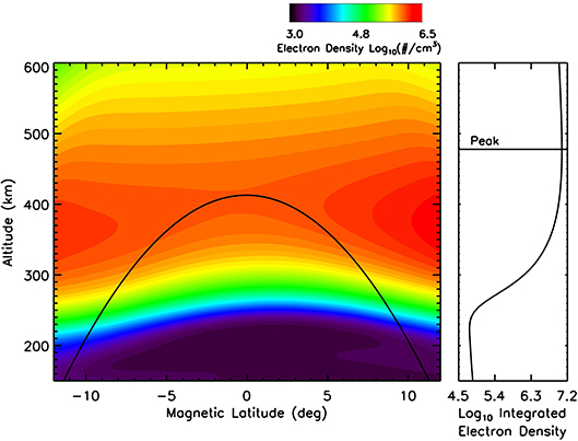
Figure 1. The (Left) shows the electron density (log₁₀ cm⁻³) as a function of latitude and altitude at 0° longitude. The black line denotes a field line with an apex of about 400 km altitude. The (Right) shows the field line integrated electron density as a function of altitude. The peak of the integrated electron density occurs around 480 km altitude.

Figure 2 shows an example of the evolution of a plasma release in the ionosphere. At 19:36 local time (LT) a Gaussian blob of 5.0 × 10⁷ cm⁻³ Al⁺ ions are released into the simulation at 200 km altitude, at location 9.9° latitude and 0° longitude. Over the next two and a half hours, the ions spread along the field line, extending between 150–300 km altitude. In addition, the extended cloud drifts downwards. Figure 3 shows a similar example of a plasma release, but at the apex of the field line (400 km altitude, 0° latitude, 0° longitude). The ions quickly fall down along the field line, extending out to ±2° latitude within 30 minutes. The cloud also begins to drift downward due to the polarization electric field generated by the plasma cloud. Generally, the larger the plasma release is, the stronger the polarization field becomes, so the denser a plasma clouds is the more quickly it will fall. It should be noted that although these particular simulations used Al⁺ as the ion species, similar simulations have been performed with Lithium ions and the results were qualitatively the same.

FIGURE 2

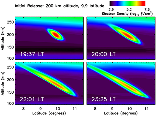
Figure 2. Electron density (log₁₀ cm⁻³) as a function of latitude and altitude at four times during the simulation. At 19:30 LT, 5.0 × 10⁷ cm⁻³ Al⁺ ions are released at 200 km altitude, 9.9° latitude. The plasma spreads along the field line (as shown in the Top right and Bottom left), then the structure begins to drift downwards.

FIGURE 3

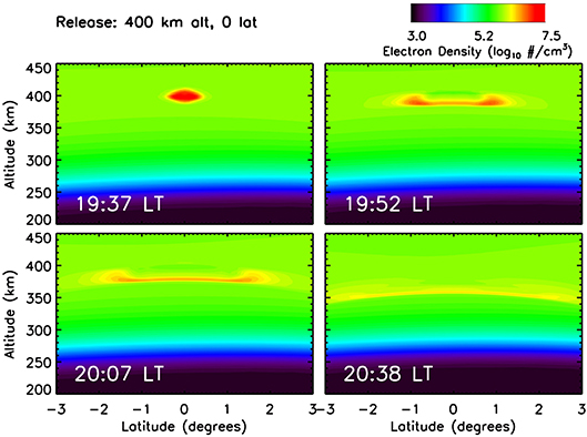
Figure 3. Electron density (log₁₀ cm⁻³) as a function of latitude and altitude at four times during the simulation. At 19:30 LT 5.0 × 10⁷ cm⁻³ Al⁺ ions are released at 400 km altitude, 0° latitude. The plasma spreads along the field line (as shown in the Top right and Bottom left), then the structure begins to drift downwards.

Figures 2, 3 show releases of Aluminum ions at different locations along the same field line. Although the growth rate of an ESF bubble is dependent on field line integrated quantities, the altitude where the plasma release occurs drastically affects both the Pedersen conductance and growth rate. The growth rate of an ESF bubble can be calculated as in Zawdie and Huba (2014):

$\begin{array}{rc}\gamma =-\frac{\int {\sigma }_{H_c}(g_p/L_n)ds}{\int {\sigma }_{p}ds}& (2)\end{array}$

where g_p is the gravitation term, s is in the direction of the field line, $L_n^{-1}=\partial ln(n_0)/\partial p$, n₀ is the electron density, p is perpendicular to the field line, σ_p is Pedersen conductivity, and σ_Hc is Hall conductivity. The Pedersen and Hall conductivities can be approximated as:

$\begin{array}{rc}{\sigma }_P\approx {\displaystyle \sum _i}\frac{nec}{B}\frac{{\nu }_{in}}{{\Omega }_i}& (3)\end{array}$

$\begin{array}{rc}{\sigma }_{H_c}\approx {\displaystyle \sum _i}\frac{nec}{B}\frac{1}{{\Omega }_i}& (4)\end{array}$

where ν_in is the ion-neutral collision frequency, Ω_i = eB/m_ic, n is the electron density, e is the electron charge, c is the speed of light, B is the magnetic field strength, and m_i is the mass of ion i. In Equation 2, ∫σ_pds is the Pedersen conductance; thus the growth rate is inversely proportional to the Pedersen conductance.

Figure 4 shows the Pedersen conductance and maximum growth rate as a function of the release altitude of the plasma injection along the field line outlined in Figure 1. The dotted line denotes the Pedersen conductance and growth rate for the background simulation case (no plasma release). The top panel shows that the lower the release altitude, the larger the increase in Pedersen conductance. Plasma releases above 300 km altitude do not have a substantial effect on the Pedersen conductivity. On the other hand, the bottom panel shows that the higher the release altitude, the larger the increase in the ESF growth rate. Plasma releases below 250 km do not significantly increase the ESF growth rate. Based on the Pedersen conductivity and growth rate change with altitude, we selected our plasma release altitudes along the selected magnetic field line for ESF bubble control. The following sections describe the plasma release simulations designed to test whether the perturbation of the Pedersen conductance/growth rate can suppress/trigger ESF bubbles.

FIGURE 4

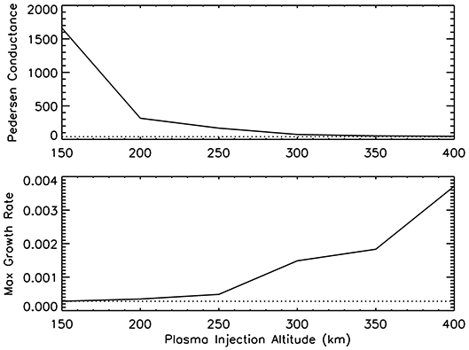
Figure 4. The Top shows the Pedersen conductance (mho) of the field line outlined in the left panel of Figure 1 for simulations with plasma releases at different altitudes. In each simulation 5.0 × 10⁷ Al⁺ ions were released at a different location along the field line. The dotted line denotes the Pedersen conductance for a simulation with no plasma release. The Bottom shows the maximum growth rate (s⁻¹) for a the same series of simulations as the Top. The dotted line shows the maximum growth rate for a simulation with no plasma release.

4.2. How to Trigger ESF Bubbles

As shown in Figure 4, a plasma release at the apex of the field line significantly increases the ESF growth rate. In this section, the results of a simulation where plasma is released at the apex (~ 400 km) of the seeding magnetic field line, are examined to determine if the increase in growth rate is sufficient to trigger the growth of an ESF bubble. The results of this numerical case study are shown in Figure 5, which shows the electron density as a function of longitude and altitude at 0° latitude. The left panels show the ambient electron density from the background simulation with no plasma release. The right panels show the simulation results for a release of 5.0 × 10⁹ cm⁻³ Al⁺ at 400 km altitude. In the top right panel, the plasma release is seen as a white blob (the color scale is saturated) at 400 km altitude just after the release. The lower panels show the evolution of the system after two and a half hours. In the background case (left), no ESF bubble forms, but in the plasma release simulation (right), an ESF bubble has been triggered and is rising through the ionosphere. Thus, by releasing plasma at the apex of the field line, an ESF bubble has been triggered.

FIGURE 5

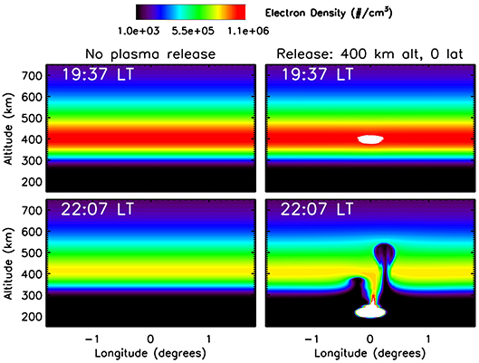
Figure 5. Electron density (log₁₀ cm⁻³) as a function of longitude and altitude at 0° latitude for two different simulations (Left, Right) at two different times (top and bottom). The left panels show the time evolution for the background simulation with no plasma release; in this case no ESF develops. The right panels show the case where a plasma release is simulated at 400 km altitude and 0° latitude. Note that the color bar saturates in the area of the plasma release. As shown in Figure 3 the plasma release spreads along the field line and then drifts downward. The bottom right panel shows that after several hours ESF bubbles develop in the ionosphere as a result of the plasma release.

Further investigations have indicated that there is a minimum plasma release density required to trigger an ESF bubble. Figure 6 shows the maximum growth rate that results from plasma releases of different densities at 400 km altitude. The larger the plasma release density, the larger the maximum growth rate. A plasma release of 5.0 × 10⁷ cm⁻³ Al⁺ ions was found to be sufficient to generate ESF, but the bubble formed more slowly in the ionosphere (3.5 h) than with a release of 5.0 × 10⁹ cm⁻³ Al⁺ (2.5 h). In our investigation, we also found that a plasma release at a lower altitude (such as 350 km) could trigger ESF, but the density threshold increases as the release altitude decreases. The numerical case study of the plasma releases below 250 km altitude are examined in the following section.

FIGURE 6

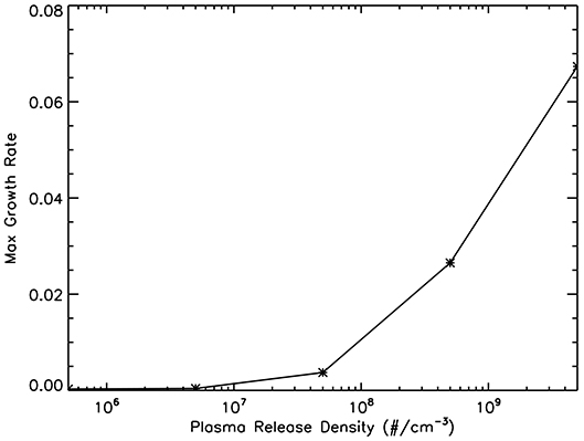
Figure 6. The maximum growth rate in the simulation as a function of injected plasma (Al⁺)density.

4.3. How to Suppress ESF Bubbles

Figure 4 shows that adding a plasma release at a lower altitudes along the seeding field line can substantially increase the Pedersen conductance. The ESF growth rate is inversely proportional to the Pedersen conductance, so it is not unreasonable to suggest that a plasma release at a low altitude (around 200 km) may suppress ESF. In this section, simulation results are examined to determine if it is feasible to suppress ESF bubbles via plasma releases. Two simulations were performed; the first had a density depletion along the seeding field line that is typically used to trigger ESF bubbles in simulations. The second had a density depletion and a plasma release of 5.0 × 10⁷ cm⁻³ Al⁺ ions at 200 km altitude, 9.9° latitude, and 0° longitude. Figure 7 shows the results of the two simulations: the electron density as a function of longitude and altitude. The left panels show the results with no plasma release and the right panels show the result of injecting plasma.

FIGURE 7

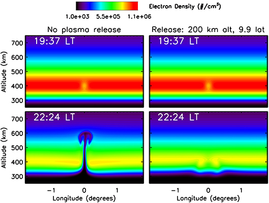
Figure 7. Electron density (log₁₀ cm⁻³) as a function of longitude and altitude at 0° latitude for two different simulations (Left and Right) at two different times (Top and Bottom). The left panels show the time evolution for the background simulation with a density depletion, but no plasma release; in this case ESF develops after several hours. The right panels show the case where a plasma release is simulated at 200 km altitude and 9.9° latitude. Note that the plasma release is not visible in this picture because it is at a different latitude. As shown in Figure 2 the plasma spreads along the field line and then drifts downward. The bottom right panel shows that no ESF bubbles develop, even after several hours, as a result of the plasma release.

The top two panels show the results shortly after the simulations begin. In both the ambient and plasma release cases, an electron density depletion in the seeding field line at 400 km altitude, 0° longitude is clearly visible. Note that the plasma release does not appear on this plot because it is at a different latitude (9.9° latitude) not covered in this figure. The bottom two panels show the results after 3 h. The simulation case with only the density depletion (left) shows a well developed ESF bubble. The case with the density depletion and the plasma release shows some density perturbations in F region around 0° longitude, but the ESF bubble has successfully been suppressed.

Further simulations indicate that there is a minimum size and density for a plasma release to suppress such a ESF bubble. In order to suppress an ESF bubble, the plasma release must cover the field lines associated with the density depletion that seeds the bubble. In this case, the density depletion and the plasma release both covered 15 and 35 km in the longitude and latitude directions, respectively. The larger the density depletion is, the larger the plasma release needs to be. The plasma release also needs to be in a suitable location in order to affect all field lines that have been perturbed by the density depletion. In addition to these constraints, there is a threshold (lower limit) where the plasma release is not dense enough to suppress an ESF bubble. This is depicted in Figure 8; it shows the Pedersen conductance as a function of plasma release density, which increases with decreasing plasma release altitude. A release of less than 5.0 × 10⁶ cm⁻³ Al⁺ ions does not increase the Pedersen conductance enough to suppress the ESF bubble. It should be noted that this threshold is lower for releases at lower altitudes, although a release below 150 km has not been examined by this study.

FIGURE 8

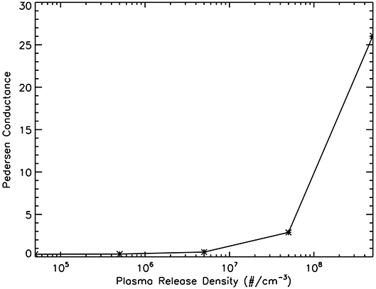
Figure 8. The Pedersen conductance as a function of injected plasma (Al⁺) density.

5. Conclusions

The numerical investigations of the present study suggest that plasma releases can be used to trigger and suppress ESF bubbles. These results are achieved by injecting plasma at different locations along a key “seeding field line" which has been used in simulations to trigger ESF. This particular field line is located below the peak of the field-line integrated electron density. Plasma releases at or near the apex of the magnetic field line spread down the field line, then the cloud drifts down to lower altitude; in the process, an ESF bubble is triggered. A plasma release at a lower altitude along the same field line can suppress an ESF bubble, provided that the plasma cloud covers all field lines affected by the ESF seed. The key challenges to manipulating the growth of ESF are ensuring that the initial plasma release is dense enough to affect the Pedersen conductance or growth rate and that the release occurs in the correct place. One obvious question is: how practical are these mechanisms for controlling ESF bubbles?

Based on the results of this numerical investigation, triggering ESF bubbles via high altitude plasma releases is likely a feasible project, however, the key engineering issue is ensuring that the injected plasma density is larger than 5.0 × 10⁹cm⁻³ ions. In order to trigger an ESF with plasma injection, the plasma must be injected at suitable location (magnetic equator) and time (19:30 LT) as we found in our test cases. Since the plasma cloud creates a polarization electric field and drifts down in altitude, the only difficulty would be ensuring that the release occurs above the F-peak and that it is timed correctly. If the release occurs at too low of an altitude, it may fail to trigger the ESF, but as long as the release occurs above the F-peak, the cloud should drift down through the region where it can trigger ESF.

Suppressing ESF in the ionosphere is likely more difficult. In addition to the constraint that the plasma releases be dense enough to adequately modify the Pedersen conductance, there are also significant limitations on the location of the plasma injection. In particular, the injection must create a plasma cloud that extends over all field lines affected by potential ESF triggers. In our numerical experiment the plasma cloud was 15 km in the longitudinal direction by 35 km in the latitudinal direction, but that only worked because the exact location and size of the density depletion was known. It is possible that with additional measurements, one could determine the most likely position of a seeding field line in a particular longitude sector. Then it is necessary that the plasma cloud extend in latitude and longitude enough to cover any potentially affected field lines.

Another complication is the presence of the neutral wind in the thermosphere. The neutral wind directly affects the growth of ESF bubbles in the ionosphere as shown in Krall et al. (2009) and Huba and Krall (2013), but the neutral wind also affects the distribution of plasma releases in the ionosphere. This is primarily an issue for attempting to suppress ESF bubbles, as the plasma release may be driven by the neutral winds to other longitude sectors, making the determination of where to put the plasma release even more difficult. A full examination of the effect of neutral winds on plasma releases in the ionosphere and their effect on the growth/suppression of ESF is left for future work.

Our analysis is also relevant to extending and controlling the transverse to the magnetic field size of high kinetic beta (β = 10³ − 10⁷) plasma injections in the ionosphere using the capabilities of the ENIG Magneto-Hydrodynamic Flux Compression Generator (FCG) (Kim and Bentz, 2015). Initial tests of this new technology have been promising and demonstrate that it may be possible to control the size of a plasma release in the near future, potentially enabling technologies to suppress ESF bubbles.

Data Availability

The datasets generated and analyzed for this study available on request from the lead author.

Author Contributions

KZ performed the model runs, generated the figures, and wrote the paper. JH assisted with the model simulations and wrote part of the paper. MD wrote part of the paper. KP guided the initial work and wrote part of the paper.

Funding

KZ and JH were supported by Chief of Naval Research (CNR) under theNRL 6.1 Base Program. This work was conducted while MD held a National Research Council's Research Associateship at Naval Research Laboratory, Washington, DC. KP was supported by AFOSR Grant No. F9550-14-1-0019 and by AFRL Contract No. FA9453-16-C-051.

Conflict of Interest Statement

The authors declare that the research was conducted in the absence of any commercial or financial relationships that could be construed as a potential conflict of interest.

References

Abdu, M. (2012). Equatorial spread F/plasma bubble irregularities under storm time disturbance electric fields. J. Atmos. Solar-Terrestrial Phys. 75-76, 44–56. doi: 10.1016/j.jastp.2011.04.024

CrossRef Full Text | Google Scholar

Abdu, M. A., Alam Kherani, E., Batista, I. S., de Paula, E. R., Fritts, D. C., and Sobral, J. H. A. (2009). Gravity wave initiation of equatorial spread F/plasma bubble irregularities based on observational data from the SpreadFEx campaign. Ann. Geophys. 27, 2607–2622. doi: 10.5194/angeo-27-2607-2009

CrossRef Full Text | Google Scholar

Berkner, L. V. and Wells, H. W. (1934). F-region ionosphere-investigations at low latitudes. J. Geophys. Res. 39, 215–230.

Google Scholar

Bernhardt, P. A. (1992). Probing the magnetosphere using chemical releases from the combined release and radiation effects satellite. Phys. Fluids B Plasma Phys. 4, 2249–2256.

Google Scholar

Burke, W. J., Huang, C. Y., Valladares, C. E., Machuzak, J. S., Gentile, L. C., and Sultan, P. J. (2003). Multipoint observations of equatorial plasma bubbles. J. Geophys. Res. Sp. Phys. 108:1221. doi: 10.1029/2002JA009382

CrossRef Full Text | Google Scholar

Çakir, S., Haerendel, G., and Eccles, J. V. (1992). Modeling the ionospheric response to artificially produced density enhancements. J. Geophys. Res. 97, 1193–1207.

Google Scholar

Carter, B. A., Yizengaw, E., Retterer, J. M., Francis, M., Terkildsen, M., Marshall, R., et al. (2014). An analysis of the quiet time day-to-day variability in the formation of postsunset equatorial plasma bubbles in the Southeast Asian region. J. Geophys. Res. 119, 3206–3223. doi: 10.1002/2013JA019570

CrossRef Full Text | Google Scholar

Caton, R. G., Pedersen, T. R., Groves, K. M., Hines, J., Cannon, P. S., Jackson-Booth, N., et al. (2017). Artificial ionospheric modification: The metal oxide space cloud experiment. Radio Sci. 52, 539–558. doi: 10.1002/2016RS005988

CrossRef Full Text | Google Scholar

de La Beaujardière, O., Retterer, J. M., Pfaff, R. F., Roddy, P. A., Roth, C., Burke, W. J., et al. (2009). C/NOFS observations of deep plasma depletions at dawn. Geophys. Res. Lett. 36:L00C06. doi: 10.1029/2009GL038884

CrossRef Full Text | Google Scholar

Farley, D. T., Balsey, B. B., Woodman, R. F., and McClure, J. P. (1970). Equatorial spread F : implications of VHF radar observations. J. Geophys. Res. 75, 7199–7216. doi: 10.1029/JA075i034p07199

CrossRef Full Text | Google Scholar

Huang, C.-S., de La Beaujardiere, O., Roddy, P. A., Hunton, D. E., Pfaff, R. F., Valladares, C. E., et al. (2011). Evolution of equatorial ionospheric plasma bubbles and formation of broad plasma depletions measured by the C/NOFS satellite during deep solar minimum. J. Geophys. Res. Sp. Phys. 116:A03309. doi: 10.1029/2010JA015982

CrossRef Full Text | Google Scholar

Huang, C.-S., Foster, J. C., and Sahai, Y. (2007). Significant depletions of the ionospheric plasma density at middle latitudes: a possible signature of equatorial spread F bubbles near the plasmapause. J. Geophys. Res. Sp. Phys. 112:A05315. doi: 10.1029/2007JA012307

CrossRef Full Text | Google Scholar

Huang, C.-S., Kelley, M. C., and Hysell, D. L. (1993). Nonlinear Rayleigh-Taylor instabilities, atmospheric gravity waves and equatorial spread < i>F < /i>. J. Geophys. Res. 98:15631.

Google Scholar

Huba, J. D., Bernhardt, P. A., and Lyon, J. G. (1992). Preliminary study of the CRRES magnetospheric barium releases. J. Geophys. Res. 97:11.

Google Scholar

Huba, J. D., Joyce, G., and Fedder, J. A. (2000). Sami2 is another model of the ionosphere (SAMI2): a new low-latitude ionosphere model. J. Geophys. Res. Sp. Phys. 105, 23035–23053. doi: 10.1029/2000JA000035

CrossRef Full Text | Google Scholar

Huba, J. D., Joyce, G., and Krall, J. (2008). Three-dimensional equatorial spread F modeling. Geophys. Res. Lett. 35. doi: 10.1029/2008GL033509

CrossRef Full Text | Google Scholar

Huba, J. D. and Krall, J. (2013). Impact of meridional winds on equatorial spread < i>F < /i>: revisited. Geophys. Res. Lett. 40, 1268–1272. doi: 10.1002/grl.50292

CrossRef Full Text | Google Scholar

Huba, J. D., Krall, J., and Joyce, G. (2009a). Atomic and molecular ion dynamics during equatorial spread F. Geophys. Res. Lett. 36:L10106. doi: 10.1029/2009GL037675

CrossRef Full Text | Google Scholar

Huba, J. D., Ossakow, S. L., Joyce, G., Krall, J., and England, S. L. (2009b). Three-dimensional equatorial spread F modeling: zonal neutral wind effects. Geophys. Res. Lett. 36:L19106. doi: 10.1029/2009GL040284

CrossRef Full Text | Google Scholar

Hysell, D. (2000). An overview and synthesis of plasma irregularities in equatorial spread F. J. Atmos. Solar-Terrestrial Phys. 62, 1037–1056. doi: 10.1016/S1364-6826(00)00095-X

CrossRef Full Text | Google Scholar

Hysell, D. L., Kudeki, E., and Chau, J. L. (2005). Possible ionospheric preconditioning by shear flow leading to equatorial spread F. Ann. Geophys. 23, 2647–2655. doi: 10.5194/angeo-23-2647-2005

CrossRef Full Text | Google Scholar

Hysell, D. L., Larsen, M. F., Swenson, C. M., Barjatya, A., Wheeler, T. F., Bullett, T. W., et al. (2006). Rocket and radar investigation of background electrodynamics and bottom-type scattering layers at the onset of equatorial spread F. Ann. Geophys. 24, 1387–1400. doi: 10.5194/angeo-24-1387-2006

CrossRef Full Text | Google Scholar

Kelley, M. C., LaBelle, J., Kudeki, E., Fejer, B. G., Basu, S., Basu, S., et al. (1986). The condor equatorial spread F campaign: overview and results of the large-scale measurements. J. Geophys. Res. 91, 5487–5503.

Google Scholar

Kelley, M. C., Rodrigues, F. S., Makela, J. J., Tsunoda, R., Roddy, P. A., Hunton, D. E., et al. (2009). C/NOFS and radar observations during a convective ionospheric storm event over South America. Geophys. Res. Lett. 36:L00C07. doi: 10.1029/2009GL039378

CrossRef Full Text | Google Scholar

K. Papadopoulos, E. E. Bentz, D. (2015). “Space plasma generator for artificial ionospheric control,” The Joint Conference of 6th International Symposium on Physical Sciences in Space (ISPS-6) and 10th International Conference on Two-Phase Systems for Space and Ground Applications, Kyoto.

Klobuchar, J. A. and Abdu, M. A. (1989). Equatorial ionospheric irregularities produced by the Brazilian Ionospheric Modification Experiment (BIME). J. Geophys. Res. 94, 2721–2726.

Google Scholar

Krall, J., Huba, J. D., Joyce, G., and Yokoyama, T. (2010a). Density enhancements associated with equatorial spread F. Ann. Geophys. 28, 327–337. doi: 10.5194/angeo-28-327-2010

CrossRef Full Text | Google Scholar

Krall, J., Huba, J. D., Joyce, G., and Zalesak, S. T. (2009). Three-dimensional simulation of equatorial spread-F with meridional wind effects. Ann. Geophys. 27, 1821–1830. doi: 10.5194/angeo-27-1821-2009

CrossRef Full Text | Google Scholar

Krall, J., Huba, J. D., Ossakow, S. L., and Joyce, G. (2010b). Why do equatorial ionospheric bubbles stop rising? Geophys. Res. Lett. 37. doi: 10.1029/2010GL043128

CrossRef Full Text

Kudeki, E., Akgiray, A., Milla, M., Chau, J. L., and Hysell, D. L. (2007). Equatorial spread-F initiation: post-sunset vortex, thermospheric winds, gravity waves. J. Atmos. Solar-Terrestrial Phys. 69, 2416–2427. doi: 10.1016/j.jastp.2007.04.012

CrossRef Full Text | Google Scholar

Kudeki, E. and Bhattacharyya, S. (1999). Postsunset vortex in equatorial F -region plasma drifts and implications for bottomside spread- F. J. Geophys. Res. Sp. Phys. 104, 28163–28170.

Google Scholar

LaBelle, J. and Kelley, M. C. (1986). The generation of kilometer scale irregularities in equatorial spread F. J. Geophys. Res. 91, 5504–5512.

Google Scholar

Le, G., Huang, C., Pfaff, R. F., Su, S., Yeh, H., Heelis, R. A., et al. (2003). Plasma density enhancements associated with equatorial spread F : ROCSAT-1 and DMSP observations. J. Geophys. Res. 108, 1318. doi: 10.1029/2002JA009592

CrossRef Full Text | Google Scholar

Ossakow, S. L. (1981). Spread-F theories—a review. J. Atmos. Terr. Phys. 43, 437–452.

Google Scholar

Ossakow, S. L., Zalesak, S. T., and McDonald, B. E. (1978). Ionospheric modification: an initial report of artificially created equatorial spread F. Geophys. Res. Lett. 5, 691–694. doi: 10.1029/GL005i008p00691

CrossRef Full Text

Pickett, J. S., Murphy, G. B., Kurth, W. S., Goertz, C. K., and Shawhan, S. D. (1985). Effects of chemical releases by the STS 3 Orbiter on the ionosphere. J. Geophys. Res. 90, 3487–3497. doi: 10.1016/0021-9169(81)90107-0

CrossRef Full Text | Google Scholar

Retterer, J., Groves, K. M., Pedersen, T. R., and Caton, R. G. (2017). The electrodynamic effects of MOSC-like plasma clouds. Radio Sci. 52, 604–615. doi: 10.1002/2016RS006085

CrossRef Full Text | Google Scholar

Retterer, J. M. (2010a). Forecasting low-latitude radio scintillation with 3-D ionospheric plume models: 1. Plume model. J. Geophys. Res. Sp. Phys. 115:A03306. doi: 10.1029/2008JA013839

CrossRef Full Text | Google Scholar

Retterer, J. M. (2010b). Forecasting low-latitude radio scintillation with 3-D ionospheric plume models: 2. Scintillation calculation. J. Geophys. Res. Sp. Phys. 115:A03307. doi: 10.1029/2008JA013840

CrossRef Full Text | Google Scholar

Retterer, J. M. and Roddy, P. (2014). Faith in a seed: on the origins of equatorial plasma bubbles. Ann. Geophys. 32, 485–498. doi: 10.5194/angeo-32-485-2014

CrossRef Full Text | Google Scholar

Stolle, C., Lühr, H., Rother, M., and Balasis, G. (2006). Magnetic signatures of equatorial spread < i>F < /i> as observed by the CHAMP satellite. J. Geophys. Res. 111:A02304. doi: 10.1029/2005JA011184

CrossRef Full Text | Google Scholar

Su, Y.-J., Retterer, J. M., de La Beaujardière, O., Burke, W. J., Roddy, P. A., Pfaff, R. F., et al. (2009). Assimilative modeling of equatorial plasma depletions observed by C/NOFS. Geophys. Res. Lett. 36:L00C02. doi: 10.1029/2009GL038946

CrossRef Full Text | Google Scholar

Sultan, P. J. (1996). Linear theory and modeling of the Rayleigh-Taylor instability leading to the occurrence of equatorial spread F. J. Geophys. Res. Sp. Phys. 101, 26875–26891. doi: 10.1029/96JA00682

CrossRef Full Text | Google Scholar

Sultan, P. J. and Jared, P. (1994). Chemical release experiments to induce F region ionospheric plasma irregularities at the magnetic equator. Ph.D. Thesis Bost. Univ. MA.

Google Scholar

Takahashi, H., Taylor, M. J., Pautet, P.-D., Medeiros, A. F., Gobbi, D., Wrasse, C. M., et al. (2009). Simultaneous observation of ionospheric plasma bubbles and mesospheric gravity waves during the SpreadFEx Campaign. Ann. Geophys. 27, 1477–1487. doi: 10.5194/angeo-27-1477-2009

CrossRef Full Text | Google Scholar

Tsunoda, R. T. (1983). On the generation and growth of equatorial backscatter plumes: 2. Structuring of the west walls of upwellings. J. Geophys. Res. 88, 4869—4874. doi: 10.1029/JA088iA06p04869

CrossRef Full Text | Google Scholar

Wan, X., Xiong, C., Rodriguez-Zuluaga, J., Kervalishvili, G. N., Stolle, C., and Wang, H. (2018). Climatology of the occurrence rate and amplitudes of local time distinguished equatorial plasma depletions observed by swarm satellite. J. Geophys. Res. 123, 3014–3026. doi: 10.1002/2017JA025072

CrossRef Full Text | Google Scholar

Woodman, R. F. (2009). Spread F – an old equatorial aeronomy problem finally resolved? Ann. Geophys. 27, 1915–1934. doi: 10.5194/angeo-27-1915-2009

CrossRef Full Text

Woodman, R. F. and La Hoz, C. (1976). Radar observations of F region equatorial irregularities. J. Geophys. Res. 81, 5447–5466.

Google Scholar

Wright, J. W. (1964). Ionosonde studies of some chemical releases in the ionosphere. Radio Sci. 68:189.

Google Scholar

Yizengaw, E. and Groves, K. M. (2018). Longitudinal and seasonal variability of equatorial ionospheric irregularities and electrodynamics. Space Weather 16, 946–968. doi: 10.1029/2018SW001980

CrossRef Full Text | Google Scholar

Zalesak, S. and Ossakow, S. (1980). Nonlinear equatorial spread F: spatially large bubbles resulting from large horizontal scale initial perturbations. J. Geophys. Res. 85:2131. doi: 10.1029/JA085iA05p02131

CrossRef Full Text | Google Scholar

Zalesak, S. T., Ossakow, S. L., and Chaturvedi, P. K. (1982). Nonlinear equatorial spread F: the effect of neutral winds and background Pedersen conductivity. J. Geophys. Res. 87:151. doi: 10.1029/JA087iA01p00151

CrossRef Full Text | Google Scholar

Zawdie, K. A. and Huba, J. D. (2014). Can HF heating generate ESF bubbles? Geophys. Res. Lett. 41, 8155–8160. doi: 10.1002/2014GL062293

CrossRef Full Text

Zawdie, K. A., Huba, J. D., and Wu, T.-W. (2013). Modeling 3-D artificial ionospheric ducts. J. Geophys. Res. Sp. Phys. 118, 7450–7457. doi: 10.1002/2013JA018823

CrossRef Full Text | Google Scholar