Resonant Damping of Propagating Kink Waves in Non-stationary, Longitudinally Stratified, and Expanding Solar Waveguides

1. Introduction

Propagating kink waves have been observed in many magnetic waveguides in the solar atmosphere, like coronal magnetic loops (Tomczyk et al., 2007; Tomczyk and McIntosh, 2009), spicules (De Pontieu et al., 2007; He J. et al., 2009; He J.-S. et al., 2009), fine structures of prominences (Okamoto et al., 2007), and in filament threads (Lin et al., 2007, 2009). It was also observed that these waves damp. At present resonant absorption is considered as the most likely candidate for explaining this damping. The theoretical modeling of the spatial damping of traveling kink waves due to resonant absorption has been carried out by Terradas et al. (2010) and Verth et al. (2010) analytically, and by Pascoe et al. (2010, 2011) numerically. In all these article the simplest model of a straight magnetic tube with the density only varying in the radial direction was used.

Later mode sophisticate models were used. Soler et al. (2011a) took into account the effect of partial ionization in the single-fluid approximation. As a result, kink waves were damped by both resonant absorption and ion-neutral collisions. Soler et al. (2011b) studied the resonant absorption of propagating kink waves in the presence of flow. Soler et al. (2011c) investigated the propagation and resonant absorption of kink waves in a magnetic tube with the density varying both along and across the tube. They showed that the variation of the wave amplitude along the tube is determined by the combined effect of resonant damping and the longitudinal density variation. Ruderman et al. (2010) studied the effect of non-linearity on the resonant damping of propagating kink waves and showed that non-linearity can strongly enhance the damping efficiency.

All papers cited above used the theory of resonant damping that can be called classical. In this theory the wave amplitude decays exponentially with the distance from the place where it is driven. This result is based on the assumption that a propagating kink wave is an eigenmode of the linearized dissipative magnetohydrodynamics (MHD). In the case of standing kink oscillations (Ruderman and Roberts, 2002) showed that after the initial perturbation the kink oscillation of a perturbed magnetic tube is very well-described by an eigenmode of the linear dissipative MHD after a transitional time of order of the oscillation period everywhere but in a vicinity of the resonant surface. However, in the vicinity of the resonant surface phase mixing continues until it creates perturbations with so small spatial scale that viscosity and/or resistivity stops it. Only after that the perturbation is described by an eigenmode of the linear dissipative MHD everywhere. It was shown numerically that, for typical parameters of coronal magnetic loops, the time when the phase mixing stops is at least by an order of magnitude larger than the typical damping time of kink oscillations (Arregui, 2015).

Hence, we conclude that the main assumption of the classical theory of resonant damping is not satisfied. This problem was addressed numerically by Pascoe et al. (2012, 2013), and analytically by Hood et al. (2013). It was shown that at the initial stage the amplitude variation with the distance from the driver is described by the Gaussian profile. And only later the amplitude decays exponentially. As a result, the damping length of a kink wave is somewhat longer than that predicted by the classical theory of resonant damping. Hence, to correctly describe the spatial damping of propagating kink waves we need to use the advanced theory developed by Hood et al. (2013). The importance of Gaussian damping strongly depends on the thickness of the transitional layer where the density drops from large value inside the tube to low value in the surrounding plasma. It also depends on the ratio of densities inside and outside the tube. The distance where the transition from the Gaussian to exponential damping occurs reduces fast when the thickness of the layer decreases, and also when the ratio of densities increases.

Ruderman and Terradas (2013) carried out an analytical analysis of resonant damping of standing kink waves similar to that made by Hood et al. (2013) for propagating kink waves. They, in particular, concluded that the classical theory of resonant damping underestimates the damping time. But, for typical values of coronal magnetic loop parameters, the error never exceeds 20%. Although a similar estimate was not obtained for propagating kink waves, on the basis of the analogy between the spatial damping of propagating waves and temporal damping of standing waves, we believe that, although the classical theory of resonant damping underestimates the damping length, the error is quite moderate. On the other hand, the advanced theory of resonant damping is much more complex than the classical theory. Hence, in this article we will use the classical theory of resonant damping.

Sometime it is observed that waveguides in the solar atmosphere are non-stationary. For example, Aschwanden and Terradas (2008) and Aschwanden and Schrijver (2011) reported observations of kink oscillations of cooling coronal loops. Inspired by these observations Ruderman (2011b) and Shukhobodskiy et al. (2018) studied the resonant damping of kink oscillations of cooling coronal magnetic loops. Morton et al. (2010) and Ballester et al. (2018) investigated the propagation of magnetosonic waves in a cooling plasma. In our paper we extend their analysis to propagating kink waves in non-stationary magnetic flux tubes. In particular, we study the kink wave propagation in cooling coronal loops.

Our article is organized as follows. In the next section we formulate the problem and present the governing equations. In section 3 we derive the equation governing the evolution of kink waves propagating along non-stationary magnetic tubes. In section 4 we derive the expression determining resonant damping of kink waves. In section 5 we derive the equation for the wave amplitude. In section 6 we consider kink wave propagation in static and non-expanding magnetic tubes. In section 7 we study kink wave propagation in non-stationary and expanding magnetic tubes. Finally, in section 8 we summarize the results obtained in the paper.

2. Problem Formulation and Governing Equations

We study propagating kink waves along a straight magnetic tube with the circular cross-section of variable radius (see Figure 1). The characteristic radius of the tube cross-section is R_*. Since the tube expands the magnetic field is spatially dependent, but the scale of its spatial variation is L_* ≫ R_*. This assumption implies that we consider a thin magnetic tube. Below we use cylindrical coordinates r, φ, z with the z-axis coinciding with the tube axis. We consider an axisymmetric equilibrium meaning that all equilibrium quantities are independent of φ. The magnetic field is not twisted meaning that its azimuthal component is zero. Its radial and axial components are expressed in terms of the magnetic flux function ψ as

$\begin{array}{ll}{B}_r=-\frac{1}{r}\frac{\partial \psi }{\partial z},B_z=\frac{1}{r}\frac{\partial \psi }{\partial r}.& (2.1)\end{array}$

FIGURE 1

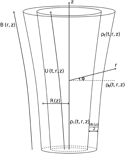
Figure 1. Sketch of the equilibrium.

Ruderman et al. (2017) (Paper I in what follows) showed that in the thin tube approximation

$\begin{array}{ll}\psi =\frac{1}{2}{r}^{2}h(z).& (2.2)\end{array}$

This expression is valid both in the tube and in its immediate surrounding.

It follows from Equations (2.1) to (2.2) that

$\begin{array}{ll}{B}_r=-\frac{1}{2}r{h}^{\prime }(z),B_z=h(z).& (2.3)\end{array}$

Since $h^{\prime }(z)~h(z)/L_{*}$, it follows that

$\begin{array}{ll}\frac{B_r}{B_z}={O}(\epsilon ),B=h(z)[1+{O}({\epsilon }^2\left)\right],& (2.4)\end{array}$

where ε = R_*/L_* and $B={(B_r^2+B_z^2)}^{1/2}$ is the magnetic field magnitude.

The plasma density varies both along and across the tube. The tube consists of a core region and a boundary layer where the density monotonically decreases from its value ρ_i inside the tube to its value ρ_e in the surrounding plasma. Here and below the indices “i” and “e” indicate that a quantity is calculated in the core region and in the surrounding plasma, respectively. The characteristic thickness of the boundary layer is lR_*, where l ≪ 1. This implies that we use the thin boundary approximation. The transitional layer boundaries are defined by equations

$\begin{array}{ll}r=R(z)(1-l/2),r=R(z)(1+l/2).& (2.5)\end{array}$

Now it follows from the magnetic flux conservation that the magnetic field tube magnitude and the tube radius are related by the approximate equation

$\begin{array}{ll}B{R}^2=\mathrm{\text{const}}.& (2.6)\end{array}$

It follows from Equations (2.2) to (2.6) that the transitional layer boundaries are magnetic field lines and their equations can be written in an alternative form as

$\begin{array}{ll}\psi ={\psi }_i\equiv \frac{1}{2}B{R}^2{\left(1-\frac{l}{2}\right)}^2,\psi ={\psi }_e\equiv \frac{1}{2}B{R}^2{\left(1+\frac{l}{2}\right)}^2.& (2.7)\end{array}$

In the core region and in the surrounding plasma the characteristic scale of density variation is L_* both in the longitudinal and radial direction. In the transitional layer the characteristic scale of density variation in the longitudinal direction is also L_*, but it is lR_* in the radial direction. The density also can depend on time. The temporal variation of density can cause the plasma flow along the magnetic field lines. Again, the velocity only weakly varies in the radial direction in the core region and outside of the tube, but it varies on the scale lR_* in the transitional layer. The density ρ and velocity U = (U_r, 0, U_z) are related by the mass conservation equation

$\begin{array}{ll}\frac{\partial \rho }{\partial t}+\frac{1}{r}\frac{\partial (\rho r{U}_r)}{\partial r}+\frac{\partial (\rho U_z)}{\partial z}=0.& (2.8)\end{array}$

Since the velocity is parallel to the magnetic field it follows from Equation (2.4) that

$\begin{array}{ll}\frac{U_r}{U_z}={O}(\epsilon ),U=U_z[1+{O}({\epsilon }^2\left)\right],& (2.9)\end{array}$

where $U={(U_r^2+U_z^2)}^{1/2}$ is the velocity magnitude. We integrate Equation (2.8) over the area of the tube core cross-section, that is over a circle of radius R(z)(1 − l/2). As a result we obtain

$\begin{array}{ll}{R}^2{(1-l/2)}^2\left(\frac{\partial \rho }{\partial t}+\frac{\partial (\rho U_z)}{\partial z}\right)+2(\rho r{U}_r){|}_{r=R(1-l/2)}=0.& (2.10)\end{array}$

It follows from Equations (2.3), (2.4), to (2.6) that hR² = const. Using this equation and Equations (2.3), (2.4), and (2.9) yields

$\begin{array}{ll}{\displaystyle \frac{U_r}{U}{|}_{r=R(1-l/2)}}={\displaystyle \frac{B_r}{B}{|}_{r=R(1-l/2)}}=-\frac{h^{\prime }R(1-l/2)}{2h}=R^{\prime }(1-l/2).& (2.11)\end{array}$

Substituting this result in Equation (2.10) we obtain in the leading order approximation with respect to ε and l

$\begin{array}{ll}\frac{\partial {\rho }_i}{\partial t}+\frac{1}{R^2}\frac{\partial ({\rho }_i{R}^2{U}_i)}{\partial z}=0.& (2.12)\end{array}$

Next we integrate (Equation 2.8) over the ring region R(1+l/2) ≤ r ≤ ςR, where ς − 1 ≫ l and ς is of the order of unity. This yields

$\begin{array}{ll}{R}^2({\varsigma }^2-1-l-l^2/4)\left(\frac{\partial \rho }{\partial t}+\frac{\partial (\rho U_z)}{\partial z}\right)+2(\rho r{U}_r){|}_{r=R(1+l/2)}^{\varsigma R}=0.& (2.13)\end{array}$

Similar to Equation (2.9) we obtain

$\begin{array}{ll}{\displaystyle \frac{U_r}{U}{|}_{r=\varsigma R}}=\varsigma R^{\prime }.& (2.14)\end{array}$

Using Equation (2.11) with −l substituted for l and (2.14) we obtain from Equation (2.13)

$\begin{array}{l}{R}^2\left({\varsigma }^2-1-l-l^2/4\right)\left(\frac{\partial \rho }{\partial t}+\frac{\partial (\rho U_z)}{\partial z}\right)\hfill \\ +2R{R}^{\prime }\left({(\rho U)|}_{\varsigma R}-{(\rho U)|}_{r=R(1+l/2)}\right)=0.\hfill \end{array}$

In the leading order approximation with respect to ε and l we neglect l in comparison with unity, and take U_z ≈ U and

$(\rho U){|}_{\varsigma R}\approx (\rho U){|}_{r=R(1+l/2)}$

in Equation (2.13). Then, dividing the obtained equation by R²(ς² − 1) yields

$\begin{array}{ll}\frac{\partial {\rho }_e}{\partial t}+\frac{1}{R^2}\frac{\partial ({\rho }_e{R}^2{U}_e)}{\partial z}=0.& (2.15)\end{array}$

It was shown in Paper I that long linear kink waves, which are waves with the wavelength much larger than R_*, in an expanding and non-stationary magnetic tube is described by the equation

$\begin{array}{l}{\rho }_i\left(\frac{\partial }{\partial t}+\frac{U_i}{R^2}\frac{\partial }{\partial z}{R}^2\right)\left(\frac{\partial \eta }{\partial t}+U_i\frac{\partial \eta }{\partial z}\right)\\ +{\rho }_e\left(\frac{\partial }{\partial t}+\frac{U_e}{R^2}\frac{\partial }{\partial z}{R}^2\right)\left(\frac{\partial \eta }{\partial t}+U_e\frac{\partial \eta }{\partial z}\right)-\frac{2B^2}{{\mu }_0}\frac{{\partial }^2\eta }{\partial z^2}={L},& (2.16)\end{array}$

where

$\begin{array}{l}{L}=\frac{\delta P}{R^2}+\frac{B^2}{{\mu }_0}\frac{{\partial }^2(l\eta +\delta \eta )}{\partial z^2}\hfill \\ -{\rho }_e\left(\frac{\partial }{\partial t}+\frac{U_e}{R^2}\frac{\partial }{\partial z}{R}^2\right)\left(\frac{\partial }{\partial t}+U_e\frac{\partial }{\partial z}\right)(ln+\delta \eta ).\hfill & (2.17)\end{array}$

In this equations μ₀ is the magnetic permeability of free space, P is the perturbation of magnetic pressure,

$\begin{array}{ll}\eta =\frac{{\xi }_{\perp i}}{R},& (2.18)\end{array}$

and ξ_⊥ is the plasma displacement in the φ = const plane and perpendicular to the magnetic field lines. In the case of non-expanding tube ξ_⊥ = ξ_r, where ξ_r is the radial component of the plasma displacement. In a slowly expanding tube ${\xi }_{\perp }={\xi }_r\left[1+{O}(\epsilon )\right]$. In the thin tube approximation ξ_⊥i is independent of r. This property is same as that first obtained in the case of non-expanding magnetic tubes (e.g., Ruderman and Erdélyi, 2009). The quantities δη and δP are the jumps across the transitional layer defined by

$\begin{array}{ll}\delta \eta =\frac{1}{R}\left({{\xi }_{\perp }|}_{\psi ={\psi }_e}-{{\xi }_{\perp }|}_{\psi ={\psi }_i}\right),\delta P={P|}_{\psi ={\psi }_e}-{P|}_{\psi ={\psi }_i}.& (2.19)\end{array}$

Equation (2.17) with the right-hand side defined by Equation (2.19) is used below to study the propagation of kink waves.

In the thin tube approximation the radial and azimuthal components of both the plasma displacement and magnetic field perturbation are independent of r inside the tube and proportional to r⁻² outside the tube. The wave energy density is equal to the sum of the kinetic and magnetic energy density. The kinetic energy density is proportional to the sum of the squares of the radial and azimuthal components of the plasma displacement, and the magnetic energy density is proportional to the sum of the squares of the radial and azimuthal components of the magnetic field perturbation. Hence, the wave energy density is independent of r inside the tube and proportional to r⁻⁴ outside the tube. The energy behavior in the boundary layer strongly depends on the dissipative coefficients and can be either monotonic or oscillatory. At distances from the place where the wave is driven that are much smaller than the damping distance the wave energy density in the transitional layer is quite small, of the order of l/R_* ≪ 1. However, at distances comparable with the damping distance almost all energy is concentrated in the transition layer due to resonant absorption.

3. Derivation of the Evolutionary Equation

In this section we consider propagation of kink waves along an expanding and non-stationary magnetic tube. Using Equations (2.12) and (2.15) we transform Equation (2.11) to

$\begin{array}{l}({\rho }_i+{\rho }_e)\frac{{\partial }^2\eta }{\partial t^2}+2\left({\rho }_i{U}_i+{\rho }_e{U}_e\right)\frac{{\partial }^2\eta }{\partial t\partial z}\\ +\left({\rho }_i{U}_i^2+{\rho }_e{U}_e^2-\frac{2B_0^2}{{\mu }_0}\right)\frac{{\partial }^2\eta }{\partial z^2}\\ +\left\{\frac{\partial }{\partial t}({\rho }_i{U}_i+{\rho }_e{U}_e)+\frac{1}{R^4}\frac{\partial }{\partial z}\left[R^4({\rho }_i{U}_i^2+{\rho }_e{U}_e^2)\right]\right\}\frac{\partial \eta }{\partial z}\\ -\left[\frac{\partial }{\partial t}({\rho }_i+{\rho }_e)+\frac{\partial }{\partial z}({\rho }_i{U}_i+{\rho }_e{U}_e)\right]\frac{\partial \eta }{\partial t}=0.& (3.1)\end{array}$

Now we consider waves with the length much longer than R_*, but much shorter than L_*. We denote the ratio of the characteristic wavelength to L_* as ϵ ≪ 1. The condition the wavelength is much larger than R_* implies that ϵ ≫ ε = R_*/L_*. We also assume that the wave period is much shorter than the characteristic scale of the temporal density variation. To study the wave propagation we look for the solution to Equation (3.1) in the form

$\begin{array}{ll}\eta =Sexp(i{ϵ}^{-1}\theta ),& (3.2)\end{array}$

where θ is real and S is complex (Bender and Orszag, 1978). The presence of transitional layer results in the resonant damping of waves. We will see below that the damping length is of the order l⁻¹ times the wavelength. On the other hand, the effect of inhomogeneity manifests itself on a distance from the place where the wave is driven that is of the order of ϵ⁻¹ times the wavelength. We would like to derive the equation for the wave amplitude that takes both effects into account in the same order approximation. In accordance with this we put l = ϵ. When l ≫ ϵ the effect of resonant absorption strongly dominates the effect of the axial density variation that can be neglected. In the opposite case where l ≪ ϵ the effect of the axial density variation strongly dominates the effect of resonant absorption. We will see below that ${L}$ is of the order of ϵ⁻¹ when l = ϵ. This estimate inspires us to introduce $\tilde{{L}}=ϵ{L}$. The characteristic time of wave damping due to resonant absorption is ϵ⁻¹ times the wave period. If the characteristic time of density variation is much larger than that time then its effect can be neglected. On the other hand, if the characteristic time of density variation is much smaller then the damping time then the effect of density variation will strongly dominate the wave damping. We aim to study the competition of the two effects. In accordance with this we assume that the ratio of the wave period to the characteristic time of density variation is of the order of ϵ. Substituting η = S exp(iϵ⁻¹θ) in Equation (3.1) and collecting terms proportional to ϵ⁻² in the obtained equation yields

$\begin{array}{ll}({\rho }_i+{\rho }_e){\omega }^2-2({\rho }_i{U}_i+{\rho }_e{U}_e)k\omega +\left({\rho }_i{U}_i^2+{\rho }_e{U}_e^2-\frac{2B_0^2}{{\mu }_0}\right)k^2=0,& (3.3)\end{array}$

where

$\begin{array}{ll}\omega =-\frac{\partial \theta }{\partial t},k=\frac{\partial \theta }{\partial z}.& (3.4)\end{array}$

This approximation is usually called the approximation of geometrical optics.

Next, we collect terms proportional to ϵ⁻¹. This results in

$\begin{array}{l}({\rho }_i+{\rho }_e)\left(S\frac{\partial \omega }{\partial t}+2\omega \frac{\partial S}{\partial t}\right)+2({\rho }_i{U}_i+{\rho }_e{U}_e)\left(S\frac{\partial \omega }{\partial z}+\omega \frac{\partial S}{\partial z}-k\frac{\partial S}{\partial t}\right)\\ -\left({\rho }_i{U}_i^2+{\rho }_e{U}_e^2-\frac{2B_0^2}{{\mu }_0}\right)\left(S\frac{\partial k}{\partial z}+2k\frac{\partial S}{\partial z}\right)\\ -\left\{\frac{\partial }{\partial t}({\rho }_i{U}_i+{\rho }_e{U}_e)+\frac{1}{R^4}\frac{\partial }{\partial z}\left[R^4({\rho }_i{U}_i^2+{\rho }_e{U}_e^2)\right]\right\}kS\\ -\left[\frac{\partial }{\partial t}({\rho }_i+{\rho }_e)+\frac{\partial }{\partial z}({\rho }_i{U}_i+{\rho }_e{U}_e)\right]\omega S=i{e}^{-i{l}^{-1}\theta }\tilde{{L}}.& (3.5)\end{array}$

Multiplying this equation by SR⁴ and using Equation (2.6) we obtain

$\begin{array}{l}{R}^4({\rho }_i+{\rho }_e)\frac{\partial (\omega S^2)}{\partial t}-R^4({\rho }_i{U}_i+{\rho }_e{U}_e)\left[\frac{\partial (k{S}^2)}{\partial t}-\frac{\partial (\omega S^2)}{\partial z}\right]\\ -\frac{\partial }{\partial z}\left[\left({\rho }_i{U}_i^2+{\rho }_e{U}_e^2-\frac{2B_0^2}{{\mu }_0}\right)k{R}^4{S}^2\right]\\ -k{R}^4{S}^2\frac{\partial }{\partial t}({\rho }_i{U}_i+{\rho }_e{U}_e)\\ -\left[\frac{\partial }{\partial t}({\rho }_i+{\rho }_e)+\frac{\partial }{\partial z}({\rho }_i{U}_i+{\rho }_e{U}_e)\right]\omega R^4{S}^2=i{e}^{-i{l}^{-1}\theta }S{R}^4\tilde{{L}}.& (3.6)\end{array}$

We further transform this equation to

$\begin{array}{l}\frac{\partial }{\partial t}\left\{R^4{S}^2\left[({\rho }_i+{\rho }_e)\omega -({\rho }_i{U}_i+{\rho }_e{U}_e)k\right]\right\}\\ +R^4({\rho }_i{U}_i+{\rho }_e{U}_e)\frac{\partial (\omega S^2)}{\partial z}-\frac{\partial }{\partial z}\left[\left({\rho }_i{U}_i^2+{\rho }_e{U}_e^2-\frac{2B_0^2}{{\mu }_0}\right)k{R}^4{S}^2\right]\\ -\left[2\frac{\partial }{\partial t}({\rho }_i+{\rho }_e)+\frac{\partial }{\partial z}({\rho }_i{U}_i+{\rho }_e{U}_e)\right]\omega R^4{S}^2\\ =i{e}^{-i{l}^{-1}\theta }S{R}^4\tilde{{L}}.& (3.7)\end{array}$

We now transform the terms on the left-hand side of this equation that are not full derivatives. Using Equations (2.12) and (2.15) we obtain

$\begin{array}{l}{R}^4({\rho }_i{U}_i+{\rho }_e{U}_e)\frac{\partial (\omega S^2)}{\partial z}\\ -\left[2\frac{\partial }{\partial t}({\rho }_i+{\rho }_e)+\frac{\partial }{\partial z}({\rho }_i{U}_i+{\rho }_e{U}_e)\right]\omega R^4{S}^2\\ =R^4({\rho }_i{U}_i+{\rho }_e{U}_e)\frac{\partial (\omega S^2)}{\partial z}\\ +\left[2({\rho }_i{U}_i+{\rho }_e{U}_e)\frac{\partial R^2}{\partial z}+R^2\frac{\partial }{\partial z}({\rho }_i{U}_i+{\rho }_e{U}_e)\right]\omega R^2{S}^2\\ =R^4({\rho }_i{U}_i+{\rho }_e{U}_e)\frac{\partial (\omega S^2)}{\partial z}+\omega S^2\frac{\partial }{\partial z}\left[R^4({\rho }_i{U}_i+{\rho }_e{U}_e)\right]\\ =\frac{\partial }{\partial z}\left[({\rho }_i{U}_i+{\rho }_e{U}_e)\omega R^4{S}^2\right].& (3.8)\end{array}$

Using this result we reduce Equation (3.7) to

$\begin{array}{l}\frac{\partial }{\partial t}\left\{R^4{S}^2\left[({\rho }_i+{\rho }_e)\omega -({\rho }_i{U}_i+{\rho }_e{U}_e)k\right]\right\}\\ +\frac{\partial }{\partial z}\left\{R^4{S}^2\left[\left({\rho }_i{U}_i+{\rho }_e{U}_e\right)\omega -\left({\rho }_i{U}_i^2+{\rho }_e{U}_e^2-\frac{2B_0^2}{{\mu }_0}\right)k\right]\right\}\\ =i{e}^{-i{l}^{-1}\theta }S{R}^4\tilde{{L}}.& (3.9)\end{array}$

Finally, introducing

$\begin{array}{ll}V=\frac{\omega }{k},{E}=R^4{S}^2\left[({\rho }_i+{\rho }_e)\omega -({\rho }_i{U}_i+{\rho }_e{U}_e)k\right],& (3.10)\end{array}$

and using Equation (3.3) we rewrite Equation (3.9) as

$\begin{array}{ll}\frac{\partial {E}}{\partial t}+\frac{\partial (V{E})}{\partial z}=i{e}^{-i{l}^{-1}\theta }S{R}^4\tilde{{L}}.& (3.11)\end{array}$

Here ${E}$ is proportional to the wave energy density per unit length along the magnetic tube.

Below we assume that the temporal variation of the density is very slow. To be specific, we consider as an example kink waves in cooling coronal loops. One observation of kink oscillation of a cooling coronal loop was reported by Aschwanden and Schrijver (2011). In this event the period of fundamental mode was 395 s, and the loop length was 163 Mm. Hence, the phase speed of the kink wave was 893 km/s. The cooling time was 2050 s. Taking this time as the characteristic time in Equation (2.12), and the loop length as the characteristic length, we obtain the estimate U_i ~ 80 km/s. Aschwanden and Schrijver (2011) did not give any information about the temperature of the plasma surrounding the loop. Cooling mainly occurs due to radiation with the intensity proportional to the plasma density squared. The plasma in the loop is much denser than that surrounding the loop. Hence, even if the external plasma cools, its cooling time is much larger than that of the plasma in the loop, and we can expect that U_e ≪ U_i. Consequently, we conclude that in the event reported by Aschwanden and Schrijver (2011) the speed of the flow induced by cooling is much smaller than the phase speed.

On the basis of this example we introduce the definition that the temporal density variation is very slow if the flow speed induced by this variation is much smaller than the phase speed. The assumption that the temporal density variation is very slow enables us to neglect the terms containing U_i and U_e in Equation (3.3). In addition, we only consider waves propagating in the positive z-direction. Then Equation (3.3) reduces to

$\begin{array}{ll}\omega =C_{k}k,C_k^2=\frac{2B^2}{{\mu }_0({\rho }_i+{\rho }_e)}.& (3.12)\end{array}$

We also can neglect the terms proportional to U_i and U_e in the expression for ${E}$ and write it in the approximate form as

$\begin{array}{ll}{E}=({\rho }_i+{\rho }_e)\omega R^4{S}^2.& (3.13)\end{array}$

4. Derivation of Expression for $\tilde{{L}}$

The assumption that the temporal variation of density is very slow enables us to use the linear equations of static MHD to describe the plasma motion in the transitional layer. However, we take the dependence of the density on time. To remove the singularity at the resonant surface we take the viscosity into account. Below we use the system of equations derived by Shukhobodskiy and Ruderman (2018). In this system ψ is used as an independent variable instead of r. Since Shukhobodskiy and Ruderman (2018) considered a static problem with the density independent on time they took the perturbation of all variables proportional to e^−iωt. However, it is easy to restore the time dependence. It suffices to substitute ∂/∂t for −iω. As a result, we obtain

$\begin{array}{ll}P=-\frac{1}{{\mu }_0}\left(r{B}^2\frac{\partial w}{\partial \psi }+i{B}^2\frac{{\xi }_{\phi }}{r}-B_r\frac{\partial w}{\partial z}+B_z\frac{w}{r}\right),& (4.1)\end{array}$

$\begin{array}{l}\frac{{\partial }^{2}w}{\partial t^2}=\frac{r{B}^2{B}_z}{{\mu }_0\rho }\frac{\partial }{\partial z}\left(\frac{B_z}{r^2{B}^2}\frac{\partial \left(rw\right)}{\partial z}\right)+\frac{B^2}{\rho }[B_r\frac{\partial }{\partial z}\left(\frac{P}{B^2}\right)\\ -r{B}^2\frac{\partial }{\partial \psi }\left(\frac{P}{B^2}\right)]+\nu \frac{\partial }{\partial t}\left(r^2{B}_z^2\frac{{\partial }^{2}w}{\partial {\psi }^2}-\frac{w}{r^2}\right),& (4.2)\end{array}$

$\begin{array}{l}\frac{{\partial }^2{\xi }_{\phi }}{\partial t^2}=-\frac{iP}{\rho r}+\frac{B_z}{{\mu }_0\rho r}\frac{\partial }{\partial z}\left[r^2{B}_z\frac{\partial }{\partial z}\left(\frac{{\xi }_{\phi }}{r}\right)\right]\\ +\nu \frac{\partial }{\partial t}\left(r^2{B}_z^2\frac{{\partial }^2{\xi }_{\phi }}{\partial {\psi }^2}-\frac{{\xi }_{\phi }}{r^2}\right).& (4.3)\end{array}$

In these equations ξ_φ is the φ-component of the plasma displacement, w = Bξ_⊥, and ν is the kinematic viscosity. We note that r is the function of ψ and z. These equations are valid both in the transitional layer as well as in the core region and external plasma where we can neglect the terms proportional to ν. The characteristic scale of variation of perturbations with respect to z is $l{\epsilon }^{-1}{R}_{*}\gg R_{*}$. The characteristic time of variation of perturbations is $l{\epsilon }^{-1}{R}_{*}/V_{*}$, where V_* is the characteristic value of the phase speed. We can take $V_{*}^2=B_{*}^2/({\mu }_0{\rho }_{*})$, where B_* and ρ_* are the characteristic values of the magnetic field and density, respectively. Using these estimates we obtain that $P~l^{-2}{\epsilon }^2{V}_{*}^2{R}_{*}^{-1}{\xi }_{\phi }$. Then the ratio of the left-hand side of Equation (4.1) to the second term in the brackets in this equation is of the order of l⁻²ε² ≪ 1, which implies that the left-hand side of Equation (4.1) can be neglected. The ratio of the third term in the brackets on the right-hand side of Equation (4.1) to the fourth term is l⁻¹ε² ≪ 1, so the third term also can be neglected. As a result, Equation (4.1) reduces to

$\begin{array}{ll}{r}^{2}B\frac{\partial w}{\partial \psi }+iB{\xi }_{\phi }+w=0.& (4.4)\end{array}$

Finally, since in the core region the dependence of both B and ξ_⊥ on ψ can be neglected, in this region we also can drop the first term in Equation (4.4).

In the WKB method all dependent variables must have the same functional form. In accordance with this, recalling that η = S exp(iϵ⁻¹θ) and l = ϵ, we put

$\begin{array}{ll}w=\widehat{w}{e}^{i{l}^{-1}\theta },{\xi }_{\phi }={\widehat{\xi }}_{\phi }{e}^{i{l}^{-1}\theta },P=\widehat{P}{e}^{i{l}^{-1}\theta }.& (4.5)\end{array}$

Using the relations w = Bξ_⊥, η = ξ_⊥i/R and η = S exp(iϵ⁻¹θ), and taking into account that the dependence of ξ_⊥ on ψ in the core region can be neglected we obtain the expression valid in the core region,

$\begin{array}{ll}{\widehat{w}}_i=BRS.& (4.6)\end{array}$

Substituting Equations (4.5) and (4.6) in Equation (4.1) with the small terms neglected, and in Equation (4.3) with ν = 0, and collecting the leading terms with respect to l we obtain the following equations valid in the core region,

$\begin{array}{ll}i{\widehat{\xi }}_{\phi }+RS=0,& (4.7)\end{array}$

$\begin{array}{ll}\widehat{P}=-i{l}^{-2}r\rho \left({\omega }^2-\frac{B^2{k}^2}{{\mu }_0\rho }\right){\widehat{\xi }}_{\phi }.& (4.8)\end{array}$

Eliminating ${\widehat{\xi }}_{\phi }$ from these equations yields

$\begin{array}{ll}\widehat{P}=l^{-2}r\rho RS\left({\omega }^2-\frac{B^2{k}^2}{{\mu }_0\rho }\right).& (4.9)\end{array}$

Now we proceed to calculating $\tilde{{L}}$. First we further simplify Equations (4.2)–(4.4). We note that we can take r(ψ, z) ≈ R(z) in the transitional layer. Using Equations (2.3) and (2.4) we also take B_z ≈ B. We can disregard the dependence of B on ψ. Finally, the characteristic scale of both the density and perturbations of all quantities in the transitional layer is ${\psi }_e-{\psi }_i=lB{R}^2$. Using these estimates we can easily show that the second term in the square brackets in Equation (4.2) strongly dominates the first term, and the second terms in brackets in terms proportional to ν are much smaller than the first terms. Finally, the ratio of the third and first terms in Equation (4.4) is of the order of l. Hence, the third term can be dropped. Then, using Equation (2.6) we reduce the system of Equations (4.2)–(4.4) to

$\begin{array}{ll}{r}^2\frac{\partial w}{\partial \psi }+i{\xi }_{\phi }=0,& (4.10)\end{array}$

$\begin{array}{ll}\frac{{\partial }^{2}w}{\partial t^2}=\frac{B^2}{{\mu }_0\rho R}\frac{{\partial }^2(wR)}{\partial z^2}-\frac{R{B}^2}{\rho }\frac{\partial P}{\partial \psi }+\nu R^2{B}^2\frac{{\partial }^{3}w}{\partial t\partial {\psi }^2},& (4.11)\end{array}$

$\begin{array}{ll}\frac{{\partial }^2{\xi }_{\phi }}{\partial t^2}=-\frac{iP}{\rho R}+\frac{R{B}^2}{{\mu }_0\rho }\frac{{\partial }^2}{\partial z^2}\left(\frac{{\xi }_{\phi }}{R}\right)+\nu R^2{B}^2\frac{{\partial }^3{\xi }_{\phi }}{\partial t\partial {\psi }^2}.& (4.12)\end{array}$

4.1. Solution Outside of the Dissipative Layer

To obtain the solution in the transitional layer we use the method of matched asymptotic expansions (e.g., Bender and Orszag, 1978). In accordance with this method we split the transitional layer in the dissipative layer and two layers sandwiching this layer where we can neglect viscosity. We look for the solution to the linear dissipative MHD in the dissipative layer and to the linear ideal MHD outside of this layer. Then we match the two solutions in the two overlap layer where the both solutions are valid. The solution in the dissipative layer is called internal, and the solution outside of the dissipative layer external.

We start from looking for the solution to the linear ideal MHD outside of the dissipative layer embracing the resonance surface defined by the equation ψ = ψ_A, where ψ_A is determined by the condition V_A(ψ_A) = C_k. Since the variation of P in the transitional layer is of the order of lP_i, we can substitute P_i(ψ = ψ_i) for P in Equation (4.12). Now, we substitute Equations (4.5) and (4.6) in Equations (4.10)–(4.12). Since we need to calculate $\tilde{{L}}$ in the leading order approximation with respect to l, we only keep leading terms. As a result, we obtain

$\begin{array}{ll}{R}^2\frac{\partial \widehat{w}}{\partial \psi }+i{\widehat{\xi }}_{\phi }=0,& (4.13)\end{array}$

$\begin{array}{ll}{k}^2\left(C_k^2-V_A^2\right)\widehat{w}=\frac{l^{2}R{B}^2}{\rho }\frac{\partial \widehat{P}}{\partial \psi },& (4.14)\end{array}$

$\begin{array}{ll}\left(C_k^2-V_A^2\right){\widehat{\xi }}_{\phi }=\frac{i{\rho }_i}{{\rho }_A}RS\left(C_k^2-V_{Ai}^2\right),& (4.15)\end{array}$

where $V_A=B{({\mu }_0\rho )}^{-1/2}$ is the Alfvén speed and ρ_A = ρ(ψ = ψ_A). When deriving Equations (4.14) and (4.15) we used the relation ω = C_kk. It follows from Equation (4.15) that

$\begin{array}{ll}{\widehat{\xi }}_{\phi }=\frac{i{\rho }_{i}RS(C_k^2-V_{Ai}^2)}{{\rho }_A(C_k^2-V_A^2)}.& (4.16)\end{array}$

We see that there is a singularity of ${\widehat{\xi }}_{\phi }$ at ψ = ψ_A(t, z). Substituting Equation (4.16) in Equation (4.13) and integrating the obtained equation yields

$\begin{array}{ll}\widehat{w}=\{\begin{array}{ll}\widehat{w}(\psi ={\psi }_i)+{\displaystyle {\int }_{{\psi }_i}^{\psi }}\frac{S(C_k^2-V_{Ai}^2)}{R(C_k^2-V_A^2)}d{\psi }_1,& \psi <{\psi }_A,\\ \widehat{w}(\psi ={\psi }_e)-{\displaystyle {\int }_{\psi }^{{\psi }_e}}\frac{S(C_k^2-V_{Ai}^2)}{R(C_k^2-V_A^2)}d{\psi }_1,& \psi >{\psi }_A.\end{array}& (4.17)\end{array}$

While ${\widehat{\xi }}_{\phi }$ has a singularity of the form ${(\psi -{\psi }_A)}^{-1}$, ŵ only has a logarithmic singularity. Finally, substituting this result in Equation (4.14) and integrating the obtained equation results in

$\begin{array}{ll}\widehat{\Phi }=\{\begin{array}{l}\widehat{\Phi }\left(\psi ={\psi }_i\right)+\frac{k^2\left(C_k^2-V_{Ai}^2\right)}{l^{2}R{B}^2}\\ {\displaystyle {\int }_{{\psi }_i}^{\psi }\left(\widehat{w}\left(\psi ={\psi }_i\right)+{\displaystyle {\int }_{{\psi }_i}^{{\psi }_1}\frac{S\left(C_k^2-V_{Ai}^2\right)}{R\left(C_k^2-V_A^2\right)}}d{\psi }_2\right)}d{\psi }_1,\psi <{\psi }_A,\\ \widehat{\Phi }\left(\psi ={\psi }_e\right)-\frac{k^2\left(C_k^2-V_{Ai}^2\right)}{l^{2}R{B}^2}\\ {\displaystyle {\int }_{\psi }^{{\psi }_e}\left(\widehat{w}\left(\psi ={\psi }_e\right)-{\displaystyle {\int }_{{\psi }_1}^{{\psi }_e}\frac{S\left(C_k^2-V_{Ai}^2\right)}{R\left(C_k^2-V_A^2\right)}}d{\psi }_2\right)}d{\psi }_1,\psi >{\psi }_A,\end{array}& (4.18)\end{array}$

where $\widehat{\Phi }$ is defined by the equation

$\begin{array}{ll}\frac{\partial \widehat{\Phi }}{\partial \psi }=\frac{1}{\rho }\frac{\partial \widehat{P}}{\partial \psi }.& (4.19)\end{array}$

It is easy to see that $\widehat{P}$ is continuous at ψ = ψ_A.

4.2. Solution Inside the Dissipative Layer

We now look for the solution in the dissipative layer embracing the resonant surface. Ruderman et al. (1995) was the first to show that solution character in the dissipative layer depends on the value of viscosity (see also Ruderman and Roberts, 2002; Goossens et al., 2011). The spatial dependence of variable perturbations in the dissipative layer is monotonic when the viscosity is not very small, while it is oscillatory for very small values of viscosity. Ruderman et al. (1995) studied a planar problem where the transition from monotonic to oscillatory behavior is determined by the relative values of two small parameters, the ratio of the thickness of transitional layer to the wavelength, and the inverse Reynolds number. He also studied the temporal damping of kink waves. However, the results that he obtained is easily translated to the spatial damping and cylindrical geometry. In this case, the variable spatial dependence is determined by the relative values of three small parameters, l, ε = R_*/L_*, and the inverse Reynolds number Re⁻¹, where Re = R_*V_*/ν. The parameter determining the character of the spatial variation of variable perturbations in the dissipative layer is l(εRe)^1/3. When l(εRe)^1/3 ≪ 1 the spatial dependence of variable perturbations in the dissipative layer is monotonic, while it is oscillatory when l(εRe)^1/3 ≳ 1. We mainly aim to apply the results of this study to the solar atmosphere, where the typical value is l ≳ 0.1, ε ≳ 0.01, while Re ≫ 10⁶, so that l(εRe)^1/3 > 1, which implies that the behavior of perturbations in the dissipative layer is oscillatory. However, in this case the equations describing the motion in the dissipative layer are very complex and, at present, it is not clear how to solve them. On the other hand, we only need to calculate the jumps of w and P across the dissipative layer. Ruderman et al. (1995) found that these jumps are independent of the value of viscosity. The only condition that must be satisfied is that Re is sufficiently large, so that the thickness of the dissipative layer is much smaller than the thickness of the transitional layer. This result was later confirmed in subsequent studies (see, e.g., the review by Goossens et al., 2011). The solution of equations describing the plasma motion in the dissipative layer in the case when l(εRe)^1/3 ≪ 1 is relatively simple. The result that the jumps of w and P across the dissipative layer are independent of l(εRe)^1/3 was obtained for a static magnetic tube with a constant cross-section radius. However, it looks like a viable conjecture to assume that this result remains correct even for a non-stationary and expanding tube. We note that the following derivation is similar to that in the case of a non-expanding tube. The only difference that in the case of a non-expanding tube we use the variable r, while in our derivation we use the variable ψ instead.

Hence, we assume that l(εRe)^1/3 ≪ 1. Since the thickness of the dissipative layer is much smaller than the thickness of the transitional layer we can approximate any equilibrium quantity in the dissipative layer by its first non-zero term of Taylor expansion with respect to ψ − ψ_A. In particular, we can substitute ρ_A = ρ(ψ = ψ_A) for ρ and take

$\begin{array}{ll}{C}_k^2-V_A^2=-\Delta (\psi -{\psi }_A),\Delta ={\displaystyle \frac{\partial V_A^2}{\partial \psi }{|}_{\psi ={\psi }_A}}.& (4.20)\end{array}$

Since we assume that the density monotonically decreases in the radial direction in the transitional layer, it follows that Δ > 0. Now, substituting Equation (4.5) in Equation (4.12), collecting terms of the order of l⁻², using Equations (4.9) and (4.20), and substituting P(ψ = ψ_i) for P we obtain

$\begin{array}{ll}\Delta (\psi -{\psi }_A){\widehat{\xi }}_{\phi }+il\nu k^{-1}{C}_k{R}^2{B}^2\frac{{\partial }^2{\widehat{\xi }}_{\phi }}{\partial {\psi }^2}=-\frac{i{\rho }_i}{{\rho }_A}RS(C_k^2-V_{Ai}^2).& (4.21)\end{array}$

When deriving this equation we took into account that ω = C_kk.

The thickness of the dissipative layer is defined by the condition that the two terms on the left-hand side of Equation (4.21) are of the same order. Using Equations (2.2) and (2.4) we easily obtain that this thickness is

$\begin{array}{ll}{\delta }_A={\left(\frac{l\nu C_k}{kRB\Delta }\right)}^{1/3}~l{R}_{*}{(\epsilon \text{Re})}^{-1/3}.& (4.22)\end{array}$

Then the condition that the thickness of the dissipative layer is much smaller than the thickness of the transitional layer reduces to εRe ≫ 1. For typical conditions in the solar atmosphere this inequality is definitely satisfied. Together with the condition that the spatial behavior of variable perturbations in the dissipative layer is non-oscillatory this gives

$\begin{array}{ll}1\ll \epsilon \text{Re}\ll l^{-3}.& (4.23)\end{array}$

The solution in the dissipative layer has to match the solution outside of this layer in the overlap layer defined by δ_A ≪ |r − r_A| ≪ lR_*. Using Equation (4.16) we obtain that the solution in the overlap layer has the form

$\begin{array}{ll}{\widehat{\xi }}_{\phi }=-\frac{i{\rho }_{i}RS(C_k^2-V_{Ai}^2)}{{\rho }_A\Delta (\psi -{\psi }_A)}+{O}\left({(\psi -{\psi }_A)}^{-2}\right).& (4.24)\end{array}$

Hence, the solution to Equation (4.21) must have this form for |ψ − ψ_A| ≫ R_*B_*δ_A. The solution to Equation (4.21) satisfying this condition is obtained in Appendix A. It is given by Equation (A6). Using Equation (A1) we rewrite it as

$\begin{array}{ll}{\widehat{\xi }}_{\phi }=-\frac{{\rho }_{i}S(C_k^2-V_{Ai}^2)}{{\rho }_{A}B\Delta {\delta }_A}F(\text{Ψ}),& (4.25)\end{array}$

where

$\begin{array}{ll}\text{Ψ}=\frac{\psi -{\psi }_A}{RB{\delta }_A},F(\text{Ψ})={\displaystyle {\int }_0^{\infty }}exp(i\sigma \text{Ψ}-\frac{1}{3}{\sigma }^3)d\sigma .& (4.26)\end{array}$

Using Equations (4.25) and (4.26) we obtain from Equation (4.13)

$\begin{array}{ll}\widehat{w}=\frac{{\rho }_{i}S(C_k^2-V_{Ai}^2)}{{\rho }_{A}R\Delta }G(\text{Ψ}),& (4.27)\end{array}$

where

$\begin{array}{ll}G(\text{Ψ})={\displaystyle {\int }_0^{\infty }}\frac{e^{i\sigma \text{Ψ}}-1}{\sigma }{e}^{-{\sigma }^3/3}d\sigma .& (4.28)\end{array}$

The functions F(Ψ) and G(Ψ) were introduced by Goossens et al. (1995).

Finally, substituting Equation (4.5) in Equation (4.11), collecting terms of the order of l⁻², and using the relation ω = C_kk, and Equations (4.20) and (4.22), and (4.26)–(4.28) we obtain

$\begin{array}{ll}\frac{\partial \widehat{\Phi }}{\partial \text{Ψ}}=\frac{{\rho }_i{k}^{2}S{\delta }_A^2(C_k^2-V_{Ai}^2)}{l^2{\rho }_A}\left(\frac{dF}{d\text{Ψ}}-\text{Ψ}G(\text{Ψ})\right).& (4.29)\end{array}$

4.3. Matching Solutions

The matching procedure is the following. First we find the asymptotic expansion of the internal solution valid for Ψ ≫ 1. Next we find the expansion of the external solution valid for $|\psi -{\psi }_A|\ll B{R}^2$. Then we substitute ψ − ψ_A = RBδ_AΨ in this expansion. The matching condition is that the leading terms of the two expansions must coincide.

We found that it is more convenient to compare not the expansions but the jumps across the dissipative layer. The jump of w across the dissipative layer is given by w(Ψ) − w(−Ψ) with Ψ ≫ 1. We obtain

$\begin{array}{l}G(\text{Ψ})-G(-\text{Ψ})=2i{\displaystyle {\int }_0^{\infty }}\frac{sin(\sigma \text{Ψ})}{\sigma }{e}^{-{\sigma }^3/3}d\sigma \\ =2i{\displaystyle {\int }_0^{\infty }}\frac{sin\sigma }{\sigma }\left[1+\left(e^{-{\sigma }^3/3{\text{Ψ}}^3}-1\right)\right]d\sigma \\ =\pi i+2i{\displaystyle {\int }_0^{\infty }}\frac{sin\sigma }{\sigma }\left(e^{-{\sigma }^3/3{\text{Ψ}}^3}-1\right)d\sigma .& (4.30)\end{array}$

It is obvious that the second term in this expression tends to zero as Ψ → ∞. Using this result we obtain from Equation (4.27) that the jump of ŵ across the dissipative layer is

$\begin{array}{ll}\widehat{w}(\text{Ψ})-\widehat{w}(-\text{Ψ})=\frac{\pi i{\rho }_{i}S(C_k^2-V_{Ai}^2)}{{\rho }_{A}R\Delta }\left[1+o(1)\right].& (4.31)\end{array}$

Using Equation (4.17) we obtain another asymptotic expression for the jump of ŵ across the dissipative layer,

$\begin{array}{ll}\widehat{w}(\psi -{\psi }_A)-\widehat{w}({\psi }_A-\psi )=\delta \widehat{w}-{P}{\displaystyle {\int }_{{\psi }_i}^{{\psi }_e}}\frac{S(C_k^2-V_{Ai}^2)}{R(C_k^2-V_A^2)}d\psi +o(1),& (4.32)\end{array}$

where δŵ = ŵ(ψ = ψ_e) − ŵ(ψ = ψ_i) and ${P}$ indicates the principal Cauchy part of an integral. This asymptotic expression is valid for |ψ − ψ_A| ≪ 1. The leading terms of the two asymptotic expressions, one given by Equation (4.31) and the other by Equation (4.32), must coincide. It follows from this condition that

$\begin{array}{ll}\delta \widehat{w}=\frac{\pi i{\rho }_{i}S(C_k^2-V_{Ai}^2)}{{\rho }_{A}R\Delta }+{P}{\displaystyle {\int }_{{\psi }_i}^{{\psi }_e}}\frac{S(C_k^2-V_{Ai}^2)}{R(C_k^2-V_A^2)}d\psi .& (4.33)\end{array}$

Now we calculate $\delta \widehat{\Phi }=\widehat{\Phi }(\psi ={\psi }_e)-\widehat{\Phi }(\psi ={\psi }_i)$. Using Equation (4.29) we obtain that the jump of P across the dissipative layer is given by

$\begin{array}{l}\widehat{\Phi }(\text{Ψ})-\widehat{\Phi }(-\text{Ψ})\\ =\frac{{\rho }_i{k}^{2}S{\delta }_A^2(C_k^2-V_{Ai}^2)}{l^2{\rho }_A}{\displaystyle {\int }_{-\text{Ψ}}^{\text{Ψ}}}\left(\frac{dF}{d{\text{Ψ}}_1}-{\text{Ψ}}_{1}G({\text{Ψ}}_1)\right)d{\text{Ψ}}_1.& (4.34)\end{array}$

The integral on the right-hand side of this equation is evaluated in Appendix B. Using Equation (B8) we obtain

$\begin{array}{ll}\widehat{\Phi }(\text{Ψ})-\widehat{\Phi }(-\text{Ψ})=-\frac{\pi i{\rho }_i{k}^{2}S{\delta }_A(C_k^2-V_{Ai}^2){\text{Ψ}}^2}{2l^2{\rho }_A}\left[1+o(1)\right].& (4.35)\end{array}$

This result and the matching condition imply that the expansion with respect to ψ − ψ_A of the jump of P across the dissipative layer calculated using the external solution must start from the term proportional to ${(\psi -{\psi }_A)}^2$. In particular, it follows from this condition that the term in this expansion proportional to unity must be zero. Using Equation (4.18) we write this condition as

$\begin{array}{l}\delta \widehat{\Phi }=\frac{k^2(C_k^2-V_{Ai}^2)}{l^{2}R{B}^2}{\displaystyle \left[{\displaystyle {\int }_{{\psi }_A}^{{\psi }_e}}\right(\widehat{w}(\psi ={\psi }_e)-{\displaystyle {\int }_{\psi }^{{\psi }_e}}\frac{S(C_k^2-V_{Ai}^2)}{R(C_k^2-V_A^2)}d{\psi }_1)d\psi }\\ {\displaystyle +{\displaystyle {\int }_{{\psi }_i}^{{\psi }_A}}(\widehat{w}(\psi ={\psi }_i)+{\displaystyle {\int }_{{\psi }_i}^{\psi }}\frac{S(C_k^2-V_{Ai}^2)}{R(C_k^2-V_A^2)}d{\psi }_1)d\psi ].}& (4.36)\end{array}$

where $\delta \widehat{\Phi }=\widehat{\Phi }(\psi ={\psi }_e)-\widehat{\Phi }(\psi ={\psi }_i)$. Since $\delta \widehat{w}/\widehat{w}={O}(l)$ and we only need to calculate $\delta \widehat{\Phi }$ in the leading order approximation with respect to l, we can substitute ŵ(ψ = ψ_e) ≈ ŵ(ψ = ψ_i) = RBS. Then, noticing that the only quantity that depends on ψ in Equation (4.36) is V_A, each single integral is of the order of l, and each double integral is of the order of l², we reduce this equation in the leading order approximation with respect to l to

$\begin{array}{ll}\delta \widehat{\Phi }=\frac{k^{2}S(C_k^2-V_{Ai}^2)({\psi }_e-{\psi }_i)}{l^{2}B}.& (4.37)\end{array}$

We note that we would obtain exactly the same expression for $\delta \widehat{\Phi }$ if we assume from the very beginning that we can neglect the jump of the pressure perturbation across the dissipative layer. This assumption was first made ad hog by Hollweg and Yang (1988). Later it was rigorously proved in 1D plasma equilibrium by Goossens et al. (1995).

Since the jump of Φ across the dissipative layer is zero, it follows that the expression for Φ obtained using the ideal MHD equations is a continuous function in the whole transitional layer. Then, using Equation (4.37) we obtain from Equation (4.18) the expression valid in the whole transitional layer in the leading order approximation with respect to l,

$\begin{array}{ll}\widehat{\Phi }=\widehat{\Phi }(\psi ={\psi }_i)+\frac{k^{2}S(C_k^2-V_{Ai}^2)(\psi -{\psi }_i)}{l^{2}B}.& (4.38)\end{array}$

When deriving this expression we neglected the second terms in the brackets in Equation (4.18) because their ratios to the first terms are of the order of l. Using Equation (4.19) we obtain

$\begin{array}{ll}\delta \widehat{P}\equiv \widehat{P}(\psi ={\psi }_e)-\widehat{P}(\psi ={\psi }_i)=\frac{k^{2}S(C_k^2-V_{Ai}^2)}{l^{2}B}{\displaystyle {\int }_{{\psi }_i}^{{\psi }_e}}\rho (\psi )d\psi .& (4.39)\end{array}$

Now we proceed to calculating $\tilde{{L}}$. We substitute η = Se^iϵ−1θ, δη = (δŵ/RB)e^iϵ−1θ, and $\delta P=\delta \widehat{P}{e}^{i{ϵ}^{-1}\theta }$ in Equation (2.17). Then, using Equation (3.12) and the condition of very slow temporal density variation implying that U_e ≪ C_k we obtain

$\begin{array}{ll}\tilde{{L}}=e^{i{ϵ}^{-1}\theta }{\displaystyle [l\frac{\delta \widehat{P}}{R^2}-\frac{1}{2}({\rho }_i-{\rho }_e){\omega }^2\left(S+l^{-1}\frac{\delta \widehat{w}}{RB}\right)]}.& (4.40)\end{array}$

Finally, using Equations (4.33) and (4.37) we arrive at

$\begin{array}{ll}\tilde{{L}}=2e^{i{ϵ}^{-1}\theta }\omega C_{k}S({\rho }_i+{\rho }_e)({\rm Y}-i\gamma ),& (4.41)\end{array}$

where

$\begin{array}{ll}\gamma =\frac{\pi k{C}_k^2{({\rho }_i-{\rho }_e)}^2}{8l{\rho }_{A}B{R}^2\Delta ({\rho }_i+{\rho }_e)},& (4.42)\end{array}$

$\begin{array}{ll}{\rm Y}=\frac{k({\rho }_i-{\rho }_e)}{4({\rho }_i+{\rho }_e)}{\displaystyle (-1+\frac{C_k^2}{l{\rho }_{i}B{R}^2}{P}{\displaystyle {\int }_{{\psi }_i}^{{\psi }_e}}\frac{\rho -{\rho }_i}{C_k^2-V_A^2}d\psi )}.& (4.43)\end{array}$

5. Derivation of Governing Equation for the Wave Amplitude

The wave evolution is described by Equation (3.11) with ${E}$ and $\tilde{{L}}$ given by Equations (3.13) and (4.41), respectively. We write S = Ae^iχ. Then, substituting Equations (3.13) and (4.41) in Equation (3.11), multiplying the obtained equation by e^−2iχ, and separating the real and imaginary parts yields

$\begin{array}{ll}\frac{\partial Q}{\partial t}+\frac{\partial (C_{k}Q)}{\partial z}=-2\gamma C_{k}Q,& (5.1)\end{array}$

$\begin{array}{ll}\frac{\partial \chi }{\partial t}+C_k\frac{\partial \chi }{\partial z}=C_k{\rm Y},& (5.2)\end{array}$

where $Q=({\rho }_i+{\rho }_e)\omega R^4{A}^2$. Equation (5.1) determines the temporal and spatial dependence of the wave amplitude, while Equation (5.2) describes a small phase shift. We are mainly interested in the variation of the wave amplitude in space and time, so we do not use Equation (5.2) below.

6. Wave Propagation Along a Static and Non-Expanding Waveguide

In this section we reproduce the results previously obtained for static and non-expanding waveguides. Hence, we assume that the tube radius is constant and equal to R.

6.1. Waveguide Homogeneous in the Axial Direction

Here we consider the same problem as that studied by Terradas et al. (2010), which is the resonant damping of kink waves propagating along a magnetic tube homogeneous in the axial direction. We now assume that the density only varies in the radial direction. We assume that a harmonic wave is driven at z = 0 and propagates in the region z > 0. In that case A is independent of time and it follows from Equation (5.1) that $A=A_0{e}^{-\gamma z}$, where A₀ is the amplitude at z = 0. Using the relation $\psi =\frac{1}{2}B{r}^2$ we obtain from Equation (4.20)

$\begin{array}{ll}\Delta ={\displaystyle -\frac{B}{{\mu }_0{\rho }_A^{2}R}\frac{d\rho }{dr}{|}_A}.& (6.1)\end{array}$

In this case both k and ω are constant. Hence, θ = kz−ωt, which implies that the wavenumber is $k_{*}=l^{-1}k$. Now, using Equation (6.1) and the relation C_k = V_A(r_A) yields

$\begin{array}{ll}\frac{\gamma }{k_{*}}=\frac{\pi {({\rho }_i-{\rho }_e)}^2}{8R({\rho }_i+{\rho }_e)|d\rho /dr{|}_A}.& (6.2)\end{array}$

This expression coincides with that obtained by Terradas et al. (2010) (see their Equation (10) with m = 1).

6.2. Waveguide With the Density Varying in the Axial Direction

Now we study the resonant damping of kink waves propagating along a magnetic tube with the density varying along the tube. This problem was first addressed by Soler et al. (2011c). We aim to reproduce their results. We assume that ρ_i(z)/ρ_e(z) = ζ = const and ρ(r, z)/ρ_e(z) = f(r). Previously these assumptions were made by Dymova and Ruderman (2006) when studying resonant damping of standing kink waves, and by Soler et al. (2011c) when studying resonant damping of propagating kink waves. We again assume that the kink wave with the amplitude A₀ and the constant frequency ω is driven at z = 0. Since now C_k is a function of z, the same is true for the wavenumber: k(z) = ω/C_k(z). Note that in non-scaled variables the wavenumber is $k_{*}(z)=l^{-1}k(z)$.

Since Q is again independent of t it immediately follows from Equation (5.1) that

$\begin{array}{ll}A=A_0\sqrt{\frac{C_k}{C_f}}exp\left(-{\displaystyle {\int }_0^z}\gamma (z_1)d{z}_1\right).& (6.3)\end{array}$

When deriving this equation we used the relation ${\rho }_i{C}_k^2={\rho }_f{C}_f^2$. Equation (6.1) remains valid. Then, using the relation ρ(r, z) = f(r)ρ_e(z) we obtain from Equation (4.42)

$\begin{array}{ll}\gamma =\frac{\omega (\zeta -1)}{2\pi {G}(\zeta +1)C_k(z)},& (6.4)\end{array}$

where

$\begin{array}{ll}{G}=\frac{4lR\left|f^{\prime }(r_A)\right|}{{\pi }^2(\zeta -1)}.& (6.5)\end{array}$

${G}=4/{\pi }^2$ for the linear density profile, and 2/π for the sinusoidal density profile. After substituting Equation (6.4) in Equation (6.3) we obtain the equation coinciding with Equation (38) in Soler et al. (2011c).

7. Wave Propagation Along an Expanding and Non-Stationary Waveguide

As an example of application of the general theory we consider a generalization of the same problem that was studied by Soler et al. (2011c), and take the loop expansion and cooling into account. We first describe the general method for studying the wave propagation, and then apply it to a particular loop with given cross-section radius and density variation along the tube, and the temporal density variation.

7.1. General Theory

We assume that a kink wave is driven at one of the loop footpoints and impose the boundary condition

$\begin{array}{ll}\omega ={\omega }_0,A=A_0\mathrm{\text{at }}z=0.& (7.1)\end{array}$

Driving starts at t = 0. Before that the loop is at rest, so we also have the initial condition

$\begin{array}{ll}A=0\mathrm{\text{at }}t=0.& (7.2)\end{array}$

The equations describing the wave propagation are solved for t > 0 and z > 0.

We start from calculating θ(t, z). It follows from dispersion Equation (3.12), ω = C_kk, and Equation (3.4) that θ(t, z) satisfies the equation

$\begin{array}{ll}\frac{\partial \theta }{\partial t}+C_k(t,z)\frac{\partial \theta }{\partial z}=0.& (7.3)\end{array}$

Since θ(t, z) is defined with the accuracy up to an additive constant we can take θ(0, 0) = 0. Then it follows from Equation (7.1) that

$\begin{array}{ll}\theta =-{\omega }_{0}t\mathrm{\text{at }}z=0.& (7.4)\end{array}$

Since the loop is at rest at t = 0 we can take

$\begin{array}{ll}\theta =0\mathrm{\text{at }}t=0.& (7.5)\end{array}$

The equation of characteristics of Equation (7.3) is

$\begin{array}{ll}\frac{dz}{dt}=C_k(t,z).& (7.6)\end{array}$

It follows from Equation (7.3) that θ = const along a characteristic. We consider the characteristic that starts at the coordinate origin. Let its equation be z = z_b(t), where z_b(0) = 0. This characteristic separates the perturbed and unperturbed regions in the (t, z)-plane, so we will call it the boundary characteristic. Let us consider a point with coordinates (t₁, z₁) satisfying the condition z₁ > z_b(t₁). This implies that this point is above the boundary characteristic. Since the characteristic containing the point (t₁, z₁) cannot intersect the boundary characteristic, it follows that it starts at the z-axis. Then, using Equation (7.5) we obtain θ(t₁, z₁) = 0.

Now we consider a point (t₁, z₁) that is below the boundary characteristic meaning that z₁ < z_b(t₁). Let the characteristic containing this point starts at t = τ(t₁, z₁) on the t-axis. Then θ(t₁, z₁) = −ω₀τ(t₁, z₁). As a result, we determine θ(t, z) in the whole region t > 0, z > 0. Differentiating θ(t, z) with respect to t we calculate ω. Then k = ω/C_k.

Next we proceed to solving Equation (5.1). The equation of characteristics of this equation is also Equation (7.6). The variation of Q along the characteristic is defined by

$\begin{array}{ll}\frac{dQ}{dt}=-\left(2\gamma C_k+\frac{\partial C_k}{\partial z}\right)Q.& (7.7)\end{array}$

After substituting in this equation a solution to Equation (7.6) found when calculating θ(t, z), Equation (7.7) becomes the equation determining the variation of Q along a characteristic. The solution to this equation must satisfy the initial condition

$\begin{array}{ll}Q=({\rho }_i+{\rho }_e){\omega }_0{R}^4{A}_0^2\mathrm{\text{at }}t=\tau (t_1,z_1).& (7.8)\end{array}$

In this equation the equilibrium quantities are calculated at t = τ and z = 0.

We now consider a point (t₁, z₁) with z₁ > z_b(t₁), which implies that it is above the boundary characteristic. In that case the characteristic that contains this point starts at the z-axis where A = 0. Then it follows that A(t₁, z₁) = 0, that is the tube is at rest for z > z_b(t). Hence, the equation z = z_b(t) describes the propagation of the wave front along the magnetic tube. Below we apply the general theory to particular cases.

7.2. Wave Propagation in Cooling and Expanding Coronal Loop

We now consider the kink wave propagation in a coronal loop of half-circle shape immersed in an isothermal atmosphere. We assume that the loop is in a vertical plane. Cooling of coronal plasma mainly occurs due to radiation. The radiation intensity is proportional to the plasma density squared. Since the plasma density inside the loop is substantially higher than that of the surrounding plasma, the plasma inside the loop cools much faster than that outside the loop. This observation inspires us to make a viable assumption that cooling only occurs inside the loop, while its temperature outside the loop does not change. Then the density inside and outside the loop is given by

$\begin{array}{ll}{\rho }_i={\rho }_{f}exp\left(-\frac{L}{\pi H(t)}sin\frac{\pi z}{L}\right),{\rho }_e=\frac{{\rho }_f}{\zeta }exp\left(-\frac{L}{\pi H_0}sin\frac{\pi z}{L}\right),& (7.9)\end{array}$

where L is the length of the loop. Following to Aschwanden and Terradas (2008) and Ruderman (2011a,b) we assume that the plasma density inside the loop decreases exponentially, so that

$\begin{array}{ll}H(t)=H_0{e}^{-t/t_c}.& (7.10)\end{array}$

Here we do not discuss the mechanisms of coronal loop cooling, although the main cause of cooling of moderately hot coronal loops with the temperature of the order of or less than 1.5 MK is the radiative cooling. Magyar et al. (2015) studied transverse oscillations of radiatively cooling coronal loops numerically. They did not present the dependence of temperature on time. However, in general their results related to the time dependence of the oscillation amplitude are in good agreement with that obtained by Ruderman (2011a,b) who assumed the exponential temperature decay. Hence, it seems that the exponential dependence of temperature on time is a reasonable approximation. The pressure inside the loop is assumed to be in equilibrium with the outside medium during the cooling. Since the plasma beta in the corona is very low this condition does not impose any serious restriction on the plasma parameters.

We adopt a model of expanding coronal loop first introduced by Ruderman et al. (2008), and later also used by Shukhobodskiy and Ruderman (2018) and Shukhobodskiy et al. (2018). In this model the cross-section radius of the magnetic tube is given by

$\begin{array}{ll}R(z)=R_f\lambda \sqrt{\frac{cosh(L/2l_c)-1}{cosh(L/2l_c)-{\lambda }^2+({\lambda }^2-1)cosh(z/l_c-L/2l_c)}}.& (7.11)\end{array}$

Here l_c is a free parameter with the dimension of length, and λ is the expansion factor equal to the ratio of the cross-section radius at the loop apex and footpoints, that is λ = R(L/2)/R_f. In our numerical study we took L/l_c = 6 and l = 0.2. Here it is worth making a comment. In section 2 we imposed the condition that L_* ≫ R_*, where L_* is the characteristic scale of the tube radius variation along the tube, and R_* is the characteristic tube radius. In the model that we adopted here L_* = l_c = L/6. Since typically L ~ 50R_*, it follows that L_*/R_* ~ 8. Hence, the condition L_* ≫ R_* is satisfied. The condition that the speed of the flow caused by cooling is much smaller than the phase speed is

$\begin{array}{ll}{N}=L{(t_c{C}_f)}^{-1}\ll 1.& (7.12)\end{array}$

In our analysis we neglect the effect of the tube curvature and consider it as straight. To our knowledge the effect of tube curvature on the propagation and damping of kink waves has not been studied. However, it was studied in the case of standing waves. Van Doorsselaere et al. (2004) analytically and Terradas et al. (2006) numerically showed that the coronal loop curvature has very minor effect on the frequency and damping of kink oscillations. It looks like a viable assumption that the same is true for propagating waves when the curvature radius is much larger than the tube radius.

The main aim of our study is to investigate the effect of cooling on the kink wave propagation. Since cooling decreases ρ_i it increases C_k. Hence, the stronger the cooling is the faster the wave perturbation launched at one footpoint at t = 0 reaches the other footpoint. We studied the wave propagation for ${N}=0$ (no cooling), ${N}=0.1$ (slow cooling), ${N}=0.2$ (moderate cooling), and ${N}=1/3$ (strong cooling). In the case of strong cooling the wave front arrives at the second footpoint at t = t_end. In all other cases the wave front arrives at the second footpoint at t > t_end. We calculated the spatial dependence of the wave frequency, wavenumber, and the amplitude at t = t_end. At z = 0 the wave frequency is $l^{-1}{\omega }_0$ and the wavenumber is $l^{-1}{\omega }_0/C_f$. In our calculation we took the wavelength at z = 0 equation to one fifth of L, that is L = 10πlC_f/ω₀ = 2πC_f/ω₀.

We introduce the dimensionless variables and parameters,

$\begin{array}{l}T=\frac{t{\omega }_0}{l},Z=\frac{z{\omega }_0}{l{C}_f},\Omega =\frac{l\omega }{{\omega }_0},K=\frac{lk{C}_f}{{\omega }_0},T_{\text{end}}=\frac{t_{\text{end}}{\omega }_0}{l},\\ \kappa =\frac{L}{\pi H_0},\alpha =\frac{{N}}{10\pi }=\frac{L}{10\pi t_c{C}_f}.& (7.13)\end{array}$

Using the relation BR² = const we obtain

$\begin{array}{ll}{C}_k^2=\frac{C_f^2{R}_f^4(\zeta +1)}{R^4\left[\zeta exp(-\kappa e^{\alpha T}sin(0.1Z))+exp(-\kappa sin(0.1Z))\right]}.& (7.14)\end{array}$

Then the characteristic Equation (7.6) reduces to

$\begin{array}{ll}\frac{dZ}{dT}=\frac{R_f^2\sqrt{\zeta +1}}{R^2\sqrt{\zeta exp(-\kappa e^{\alpha T}sin(0.1Z))+exp(-\kappa sin(0.1Z))}}.& (7.15)\end{array}$

The quantity T_end is defined by the equation $Z_b(T_{\text{end}})={\omega }_{0}L{(l{C}_f)}^{-1}$, where Z_b(T) is the solution to Equation (7.15) with α = 1/30π satisfying the initial condition Z_b(0) = 0. Using Equation (7.15) we calculated the dependence of the wave front position on time for various values of κ and λ. This dependence is shown in Figure 2. We see that the stronger the cooling is the faster the wave front moves. This results is not surprising because the cooling causes the enhancement of the phase speed C_k. We can also see that the effect of cooling is rather weak, although the tube expansion makes it more pronounced.

FIGURE 2

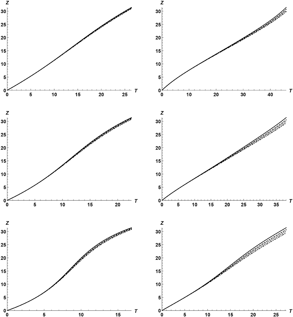
Figure 2. Dependence of the wave front position on time. The calculations continued until the wave front reaches the other end of the magnetic tube. The left panels correspond to λ = 1 and the right to λ = 1.5. The upper, middle, and lower panels correspond to κ = 0.5, κ = 1, and κ = 2, respectively. The solid, dashed, dotted, and dash-dotted curves correspond to ${N}=1/3$, ${N}=0.2$, ${N}=0.1$, and ${N}=0$, respectively.

We also calculated the dimensionless frequency Ω and wavenumber K for various values of λ, Ω, and κ. The results are presented in Figures 3, 4. First of all, we note the frequency is constant when there is no cooling as it must be. When there is cooling, in a non-expanding loop the frequency increases with the distance from the footpoint where the wave is driven. The stronger the cooling is the more pronounced this effect is. However, this effect is quite weak. The dependence of frequency on the cooling rate is much stronger in an expanding loop. We see that it is especially strong when the tube expands and the loop height substantially exceeds the atmospheric scale height. The situation with the wavenumber is quite similar. Again cooling almost does affect it in non-expanding loops, while in expanding loops the effect of cooling is quite noticeable.

FIGURE 3

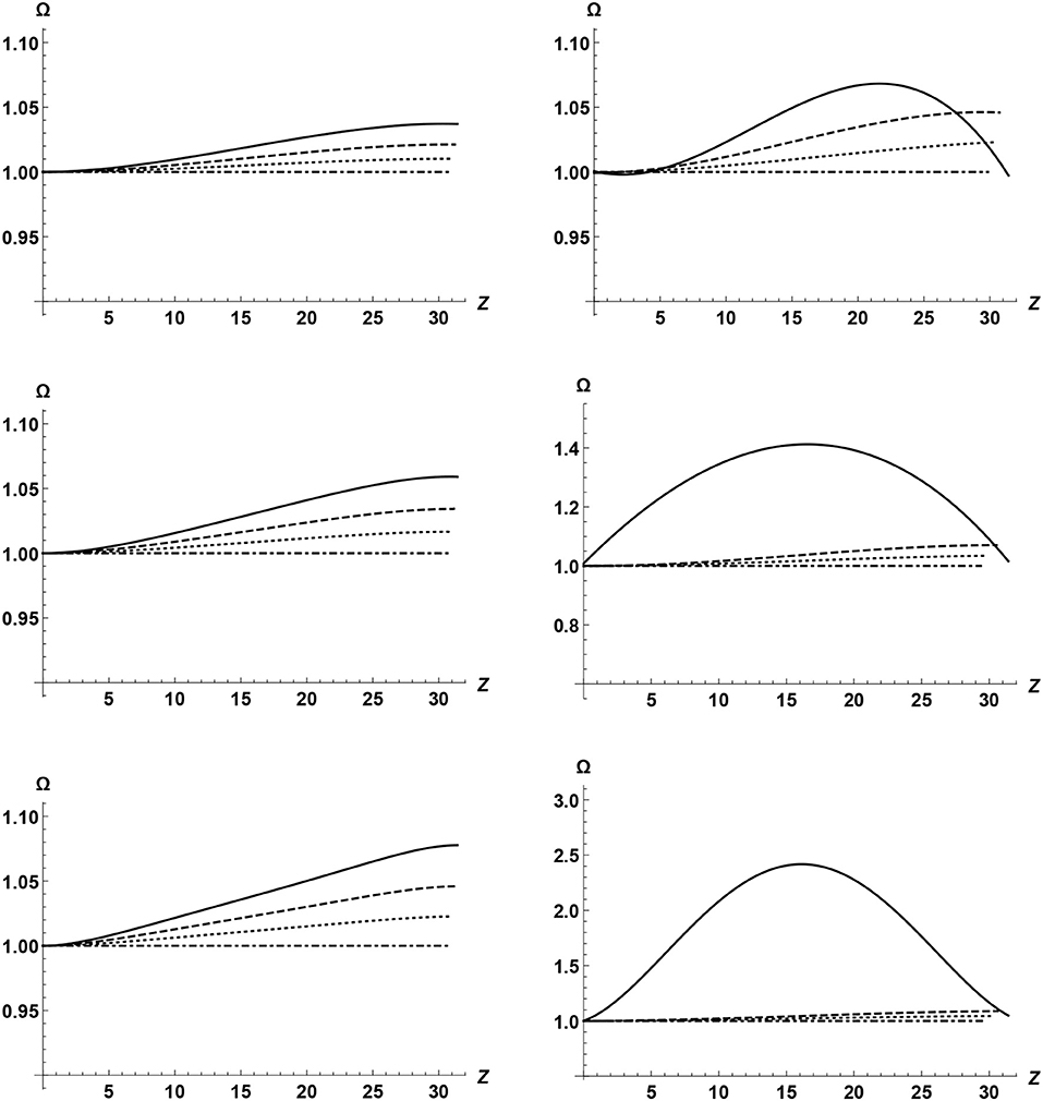
Figure 3. Dependence of the frequency on the distance along the loop for T = T_end. The left panels correspond to λ = 1 and the right to λ = 1.5. The upper, middle, and lower panels correspond to κ = 0.5, κ = 1, and κ = 2, respectively. The solid, dashed, dotted, and dash-dotted curves correspond to ${N}=1/3$, ${N}=0.2$, ${N}=0.1$, and ${N}=0$, respectively.

FIGURE 4

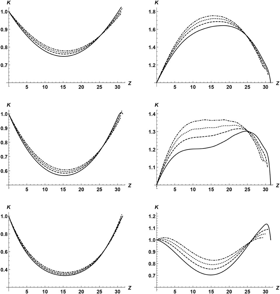
Figure 4. Dependence of the wave number on the distance along the loop for t = t_end. The left panels correspond to λ = 1 and the right to λ = 1.5. The upper, middle, and lower panels correspond to κ = 0.5, κ = 1, and κ = 2, respectively. The solid, dashed, dotted, and dash-dotted curves correspond to ${N}=1/3$, ${N}=0.2$, ${N}=0.1$, and ${N}=0$, respectively.

Finally, Figure 5 displays the variation of the amplitude along the loop. It is worth noticing that, in most cases, the amplitude first increases and then starts to decay. The amplitude increase is related with the stratification, while the decay is cased by the resonant damping. We can see that cooling always results in the amplification of waves. This result is similar to that found by Ruderman (2011a,b); Ruderman et al. (2017), and Shukhobodskiy et al. (2018) in the case of standing kink waves.

FIGURE 5

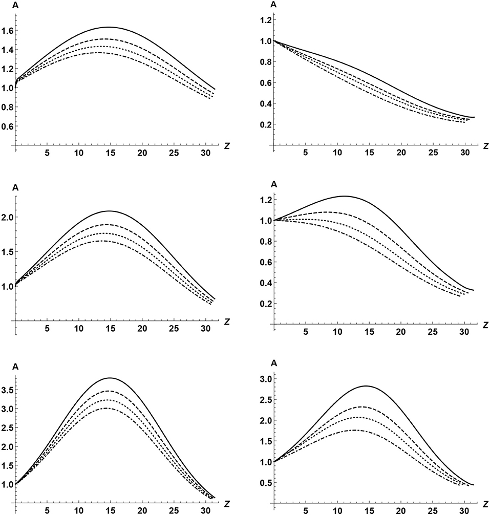
Figure 5. Dependence of the amplitude on the distance along the loop for t = t_end. The left panels correspond to λ = 1 and the right to λ = 1.5. The upper, middle, and lower panels correspond to κ = 0.5, κ = 1, and κ = 2, respectively. The solid, dashed, dotted, and dash-dotted curves correspond to ${N}=1/3$, ${N}=0.2$, ${N}=0.1$, and ${N}=0$, respectively.

8. Summary and Conclusions

In this article we studied the kink wave propagation along an expanding magnetic tube with the density varying along the tube and in time. The tube consists of the core region where the density is almost independent of the radial coordinate, and the boundary layer where the density decreasing fast from its value inside the core region to its value in the surrounding plasma. This value is assumed to be thin meaning that its thickness is much smaller than the tube radius. We used the cold plasma approximation. We also used the thin tube approximation meaning that the wave length is much larger than the tube radius, and the short wave approximation meaning that the wavelength is much smaller than the characteristic scale of the density and tube radius variation along the tube. Using the WKB method we derived the equation describing the dependence of the wave amplitude on time and on the distance along the tube.

First we studied the kink wave propagation in a magnetic tube homogeneous in the axial direction. In this case the only effect affecting the wave propagation is the wave damping due to resonant absorption. We reproduced the results previously obtained by Terradas et al. (2010).

We then proceeded to studying the kink wave propagation in a magnetic tube with the density varying in the axial direction. In this case the wave propagation are affected both by resonance absorption and the axial inhomogeneity. We reproduced the analysis by Soler et al. (2011c).

Finally, we studied the kink wave propagation in an expanding and non-stationary magnetic tube. We obtained the general expressions determining the spatial and temporal dependence of wave frequency, wavenumber, and amplitude. We then applied the general theory to a particular case of kink wave propagating along a cooling coronal loop. We assumed that the loop has a half-circle shape and immersed in an isothermal atmosphere, the temperature of plasma inside the loop decays exponentially, while the temperature of the surrounding plasma does not change. We adopted the dependence of the loop cross-section on the distance along the loop previously used by Ruderman et al. (2008, 2017) and Shukhobodskiy et al. (2018). The equations governing the wave propagation were solved numerically. We assumed that the wave was started to be driven at one of the footpoints at the same time when the plasma inside the loop started to cool. Our main aim was to study the dependence of the wave properties on the intensity of cooling. First we studied the dependence of the distance that the wavefront travels on time. We found that the stronger the cooling is the larger the distance that the wave front travel at a given time. This is an expected result because cooling enhances the phase speed thus accelerating the wavefront. We also calculated the dependence of the wave frequency and wave number on the distance along the tube. When doing so we chose the moment of time when the wavefront arrives at the second footpoint in the case of strongest cooling. The general conclusion is that cooling results in the increase of the wave frequency. In contrast, it is difficult to make any definite conclusion about the effect of cooling on the wavenumber. Finally, we investigated the dependence of the wave amplitude on the distance along the tube. In most cases the amplitude first growths due to the equilibrium quantity variation along the tube, and then its starts to decay due to resonant damping. We found that cooling enhances the wave amplitude. This result is similar to one previously obtained for standing kink waves (Ruderman, 2011a,b; Shukhobodskiy et al., 2018).

Author Contributions

All authors listed have made a substantial, direct and intellectual contribution to the work, and approved it for publication.

Conflict of Interest Statement

The authors declare that the research was conducted in the absence of any commercial or financial relationships that could be construed as a potential conflict of interest.

Acknowledgments

The authors acknowledge the support by Science and Technology Facilities Council UK (STFC), grant ST/M000826/.

References

Arregui, I. (2015). Wave heating of the solar atmosphere. Philos. Trans. R. Soc. 373:20140261. doi: 10.1098/rsta.2014.0261

PubMed Abstract | CrossRef Full Text | Google Scholar

Aschwanden, M. J., and Schrijver, C. J. (2011). Coronal loop oscillations observed with atmospheric imaging assembly – kink mode with cross-sectional and density oscillations. Astrophys. J. 736:102. doi: 10.1088/0004-637X/736/2/102

CrossRef Full Text | Google Scholar

Aschwanden, M. J., and Terradas, J. (2008). The effect of radiative cooling on coronal loop oscillations. Astrophys. J. Lett. 686, L127–L130. doi: 10.1086/592963

CrossRef Full Text | Google Scholar

Ballester, J. L., Carbonell, M., Soler, R., and Terradas, J. (2018). The temporal behaviour of MHD waves in a partially ionized prominence-like plasma: effect of heating and cooling. Astron. Astrophys. 609:A6. doi: 10.1051/0004-6361/201731567

CrossRef Full Text | Google Scholar

Bender, C. M., and Orszag, S. A. (1978). Advanced Mathematical Methods for Scientists and Engineers. New York, NY: McGraw-Hill.

Google Scholar

De Pontieu, B., McIntosh, S. W., Carlsson, M., Hansteen, V. H., Tarbell, T. D., Schrijver, C. J., et al. (2007). Chromospheric Alfvénic waves strong enough to power the solar wind. Science 318, 1574–1577. doi: 10.1126/science.1151747

PubMed Abstract | CrossRef Full Text | Google Scholar

Dymova, M. V., and Ruderman, M. S. (2006). Resonantly damped oscillations of longitudinally stratified coronal loops. Astron. Astrophys. 457, 1059–1070. doi: 10.1051/0004-6361:20065051

CrossRef Full Text | Google Scholar

Goossens, M., Erdélyi, R., and Ruderman, M. S. (2011). Resonant MHD waves in the solar atmosphere. Space Sci. Rev. 158, 289–338. doi: 10.1007/s11214-010-9702-7

CrossRef Full Text | Google Scholar

Goossens, M., Ruderman, M. S., and Hollweg, J. V. (1995). Dissipative MHD solutions for resonant Alfvén waves in 1-dimensional magnetic flux tubes. Solar Phys. 157, 75–102. doi: 10.1007/BF00680610

CrossRef Full Text | Google Scholar

He, J., Marsch, E., Tu, C., and Tian, H. (2009). Excitation of kink waves due to small-scale magnetic reconnection in the chromosphere? Astrophys. J. 705, L217–L222. doi: 10.1088/0004-637X/705/2/L217

CrossRef Full Text | Google Scholar

He, J.-S., Tu, C.-Y., Marsch, E., Guo, L.-J., Yao, S., and Tian, H. (2009). Upward propagating high-frequency Alfvén waves as identified from dynamic wave-like spicules observed by SOT on Hinode. Astron. Astrophys. 497, 425–535. doi: 10.1051/0004-6361/200810777

CrossRef Full Text | Google Scholar

Hollweg, J. V., and Yang, G. (1988). Resonance absorption of compressible magnetohydrodynamic waves at thin “surfaces”. J. Geophys. Res. 93, 5423–5436. doi: 10.1029/JA093iA06p05423

CrossRef Full Text | Google Scholar

Hood, A. W., Ruderman, M. S., Pascoe, D. J., De Moortel, I., Terradas, J., and Wright, A. N. (2013). Damping of kink waves by mode coupling I. Analytical treatment. Astron. Astrophys. 551:A39. doi: 10.1051/0004-6361/201220617

CrossRef Full Text | Google Scholar

Lin, Y., Engvold, O., Rouppe van der Voort, L. H. M., and van Noort, M. (2007). Evidence of traveling waves in filament threads. Sol. Phys. 246, 65–72. doi: 10.1007/s11207-007-0402-8

CrossRef Full Text | Google Scholar

Lin, Y., Soler, R., Engvold, O., Ballester, J. L., Langangen, Ø., Oliver, R., et al. (2009). Swaying threads of a solar filament. Astrophys. J. 704, 870–876. doi: 10.1088/0004-637X/704/1/870

CrossRef Full Text | Google Scholar

Magyar, N., Van Doorsselaere, T., and Marcu, A. (2015). Numerical simulations of transverse oscillations in radiatively cooling coronal loops. Astron. Astrophys. 582:A117. doi: 10.1051/0004-6361/201526287

CrossRef Full Text | Google Scholar

Morton, R. J., Hood, A. W., and Erdélyi, R. (2010). Propagating magneto-hydrodynamic waves in a cooling homogenous coronal plasma. Astron. Astrophys. 512:A23. doi: 10.1051/0004-6361/200913365

CrossRef Full Text | Google Scholar

Okamoto, T. J., Tsuneta, S., Berger, T. E., Ichimoto, K., Katsukawa, Y., Lites, B. W., et al. (2007). Coronal transverse magnetohydrodynamic waves in a solar prominence. Science 318, 1577–1580. doi: 10.1126/science.1145447

PubMed Abstract | CrossRef Full Text | Google Scholar

Pascoe, D. J., Hood A. W., De Moortel, I., and Wright, A. N. (2012). Spatial damping of propagating kink waves due to mode coupling. Astron. Astrophys. 539:A37. doi: 10.1051/0004-6361/201117979

CrossRef Full Text | Google Scholar

Pascoe, D. J., Hood A. W., De Moortel, I., and Wright, A. N. (2013). Damping of kink waves by mode coupling II. Parametric study and seismology. Astron. Astrophys. 551:A40. doi: 10.1051/0004-6361/201220620

CrossRef Full Text | Google Scholar

Pascoe, D. J., Wright, A. N., and De Moortel, I. (2010). Coupled Alfvén and kink oscillations in coronal loops. Astrophys. J. 711, 990–996. doi: 10.1088/0004-637X/711/2/990

CrossRef Full Text | Google Scholar

Pascoe, D. J., Wright, A. N., and De Moortel, I. (2011). Propagating coupled Alfvén and kink oscillations in an arbitrary inhomogeneous corona. Astrophys. J. 731:73. doi: 10.1088/0004-637X/731/1/73

CrossRef Full Text | Google Scholar

Ruderman, M. S. (2011a). Transverse oscillations of coronal loops with slowly changing density. Solar Phys. 271, 41–54. doi: 10.1007/s11207-011-9772-z

CrossRef Full Text | Google Scholar

Ruderman, M. S. (2011b). Resonant damping of kink oscillations of cooling coronal magnetic loops. Astron. Astrophys. 534:A78. doi: 10.1051/0004-6361/201117416

CrossRef Full Text | Google Scholar

Ruderman, M. S., and Erdélyi, R. (2009). Transverse oscillations of coronal loops. Space Sci. Rev. 149, 199–228. doi: 10.1007/s11214-009-9535-4

CrossRef Full Text | Google Scholar

Ruderman, M. S., Goossens, M., and Andries, J. (2010). Nonlinear propagating kink waves in thin magnetic tubes. Phys. Plasmas 17:082108. doi: 10.1063/1.3464464

CrossRef Full Text | Google Scholar

Ruderman, M. S., and Roberts, B. (2002). The damping of coronal loop oscillations. Astrophys.J. 577, 475–486. doi: 10.1086/342130

CrossRef Full Text | Google Scholar

Ruderman, M. S., Shukhobodskiy, A. A., and Erdélyi, R. (2017). Kink oscillations of cooling coronal loops with variable cross-section. Astron. Astrophys. 602:A50. doi: 10.1051/0004-6361/201630162

CrossRef Full Text | Google Scholar

Ruderman, M. S., and Terradas, J. (2013). Damping of coronal loop kink oscillations due to mode conversion. Astron. Astrophys. 555:A27. doi: 10.1051/0004-6361/201220195

CrossRef Full Text | Google Scholar

Ruderman, M. S., Tirry, W., and Goossens, M. (1995). Non-stationary resonant Alfvén surface waves in one-dimensional magnetic plasmas. J. Plasma Phys. 54, 129–148. doi: 10.1017/S0022377800018407

CrossRef Full Text | Google Scholar

Ruderman, M. S., Verth, G., and Erdélyi, R. (2008). Transverse oscillations of longitudinally stratified coronal loops with variable cross section. Astrophys. J. 686, 694–700. doi: 10.1086/591444

CrossRef Full Text | Google Scholar

Shukhobodskiy, A. A., and Ruderman, M. S. (2018). Resonant damping of kink oscillations of thin expanding magnetic tubes. Astron. Astrophys. 615:A156. doi: 10.1051/0004-6361/201732396

CrossRef Full Text | Google Scholar

Shukhobodskiy, A. A., Ruderman, M. S., and Erdélyi, R. (2018). Resonant damping of kink oscillations of thin cooling and expanding coronal magnetic loops. Astron. Astrophys. 619:A173. doi: 10.1051/0004-6361/201833714

CrossRef Full Text | Google Scholar

Soler, R., Oliver, R., and Ballester, J. L. (2011a). Spatial damping of propagating kink waves in prominence threads. Astrophys. J. 726:102. doi: 10.1088/0004-637X/726/2/102

CrossRef Full Text | Google Scholar

Soler, R., Terradas, J., and Goossens, M. (2011b). Spatial damping of propagating kink waves due to resonant absorption: effect of background flow. Astrophys. J. 734:80. doi: 10.1088/0004-637X/734/2/80

CrossRef Full Text | Google Scholar

Soler, R., Terradas, J., Verth, G., and Goossens, M. (2011c). Resonantly damped propagating kink waves in longitudinally stratified solar waveguides. Astrophys. J. 736:10. doi: 10.1088/0004-637X/736/1/10

CrossRef Full Text | Google Scholar

Terradas, J., Goossens, M., and Verth, G. (2010). Selective spatial damping of propagating kink waves due to resonant absorption. Astron. Astrophys. 524:A23. doi: 10.1051/0004-6361/201014845

CrossRef Full Text | Google Scholar

Terradas, J., Oliver, R., and Ballester, J. L. (2006). Damping of kink oscillations in curved coronal loops. Astrophys. J. 650, L91–L94. doi: 10.1086/508569

CrossRef Full Text | Google Scholar

Tomczyk, S., and McIntosh, S. W. (2009). Time-distance seismology of the solar corona with CoMP. Astrophys. J. 697, 1384–1391. doi: 10.1088/0004-637X/697/2/1384

CrossRef Full Text | Google Scholar

Tomczyk, S., McIntosh, S. W., Keil, S. L., Judge, P. G., Schad, T., Seeley, D., et al. (2007). Alfvén waves in the solar corona. Science 317, 1192–1196. doi: 10.1126/science.1143304

PubMed Abstract | CrossRef Full Text | Google Scholar

Van Doorsselaere, T., Debosscher, A., Andries, J., and Poedts, S. (2004). The effect of curvature on quasi-modes in coronal loops. Astron. Astrophys. 424, 1065–1074. doi: 10.1051/0004-6361:20041239

CrossRef Full Text | Google Scholar

Verth, G., Terradas, J., and Goossens, M. (2010). Observational evidence of resonantly damped propagating kink waves in the solar corona. Astrophys. J. 718, L102–L105. doi: 10.1088/2041-8205/718/2/L102

CrossRef Full Text | Google Scholar

Appendix

A. Solution to Equation (4.21)

In this section we obtain the solution to Equation (4.21) satisfying the asymptotic condition Equation (4.24). To simplify calculations we introduce the notation

$\begin{array}{ll}\text{Ψ}=\frac{\psi -{\psi }_A}{RB{\delta }_A},h=\frac{{\rho }_{i}S(C_k^2-V_{Ai}^2)}{{\rho }_{A}B\Delta {\delta }_A}.& (\mathrm{A1})\end{array}$

Using this notation we rewrite Equation (4.21) as

$\begin{array}{ll}\text{Ψ}{\widehat{\xi }}_{\phi }+i\frac{{\partial }^2{\widehat{\xi }}_{\phi }}{\partial {\text{Ψ}}^2}=-ih.& (\mathrm{A2})\end{array}$

To solve this equation we use the Fourier transform with respect to Ψ defined by

$\begin{array}{ll}{F}\left[{\widehat{\xi }}_{\phi }\right]={\displaystyle {\int }_{-\infty }^{\infty }}{\widehat{\xi }}_{\phi }{e}^{-i\sigma \text{Ψ}}d\text{Ψ},{\widehat{\xi }}_{\phi }=\frac{1}{2\pi }{\displaystyle {\int }_{-\infty }^{\infty }}{F}\left[{\widehat{\xi }}_{\phi }\right]e^{i\sigma \text{Ψ}}d\sigma .& (\mathrm{A3})\end{array}$

Applying this transform to Equation (A2) we obtain

$\begin{array}{ll}\frac{\partial }{\partial \sigma }{F}[{\widehat{\xi }}_{\phi }]+{\sigma }^2{F}[{\widehat{\xi }}_{\phi }]=-2\pi h\delta (\sigma ),& (\mathrm{A4})\end{array}$

where δ(σ) is the delta-function. The solution to this equation decaying as |σ| → ∞ is given by

$\begin{array}{ll}{F}[{\widehat{\xi }}_{\phi }]=-2\pi hH(\sigma )e^{-{\sigma }^3/3},& (\mathrm{A5})\end{array}$

where H(σ) is the Heaviside step function. Calculating the inverse Fourier transform we obtain

$\begin{array}{ll}{\widehat{\xi }}_{\phi }=-h{\displaystyle {\int }_0^{\infty }}exp(i\sigma \text{Ψ}-\frac{1}{3}{\sigma }^3)d\sigma .& (\mathrm{A6})\end{array}$

Using the integration by parts we obtain the asymptotic expression valid for |Ψ| ≫ 1,

$\begin{array}{ll}{\widehat{\xi }}_{\phi }=-\frac{ih}{\text{Ψ}}+{O}\left({\text{Ψ}}^{-2}\right).& (\mathrm{A7})\end{array}$

Using Equation (A1) it is straightforward to verify that Equation (A7) coincides with Equation (4.24).

B. Evaluation of Integral in Equation (4.34)

In this section we evaluate the integral on the right-hand side of Equation (4.34) for |Ψ ≫ 1. We immediately obtain

$\begin{array}{l}{\displaystyle {\int }_{-\text{Ψ}}^{\text{Ψ}}}\left({\text{Ψ}}_{1}G({\text{Ψ}}_1)-\frac{dF}{d{\text{Ψ}}_1}\right)d{\text{Ψ}}_1=-F(\text{Ψ})+F(-\text{Ψ})\\ +{\displaystyle {\int }_{-\text{Ψ}}^{\text{Ψ}}}{\text{Ψ}}_{1}G({\text{Ψ}}_1)d{\text{Ψ}}_1.& (\mathrm{B1})\end{array}$

It is obvious that

$\begin{array}{ll}F(\text{Ψ})-F(-\text{Ψ})=2i{\displaystyle {\int }_0^{\infty }}sin(\sigma \text{Ψ})e^{-{\sigma }^3/3}d\sigma ={O}(1).& (\mathrm{B2})\end{array}$

Changing the order of integration we obtain

$\begin{array}{ll}{\displaystyle {\int }_{-\text{Ψ}}^{\text{Ψ}}}{\text{Ψ}}_{1}G({\text{Ψ}}_1)d{\text{Ψ}}_1=2i{\displaystyle {\int }_0^{\infty }}[sin(\sigma \text{Ψ})-(\sigma \text{Ψ})cos(\sigma \text{Ψ})]\frac{e^{-{\sigma }^3/3}}{{\sigma }^3}d\sigma .& (\mathrm{B3})\end{array}$

Then, using the integration by parts yields

$\begin{array}{ll}{\displaystyle {\int }_{-\text{Ψ}}^{\text{Ψ}}}{\text{Ψ}}_{1}G({\text{Ψ}}_1)d{\text{Ψ}}_1=i{\text{Ψ}}^2{\displaystyle {\int }_0^{\infty }}\frac{sin(\sigma \text{Ψ})}{\sigma }{e}^{-{\sigma }^3/3}d\sigma +I(\text{Ψ}),& (\mathrm{B4})\end{array}$

where

$\begin{array}{ll}I(\text{Ψ})=i{\displaystyle {\int }_0^{\infty }}[(\sigma \text{Ψ})cos(\sigma \text{Ψ})-sin(\sigma \text{Ψ})]e^{-{\sigma }^3/3}d\sigma .& (\mathrm{B5})\end{array}$

Again using the integration by parts we obtain

$\begin{array}{ll}I(\text{Ψ})=i{\displaystyle {\int }_0^{\infty }}({\sigma }^3-2)sin(\sigma \text{Ψ})e^{-{\sigma }^3/3}d\sigma ={O}(1).& (\mathrm{B6})\end{array}$

With the aid of the variable substitution we obtain

$\begin{array}{ll}{\displaystyle {\int }_0^{\infty }}\frac{sin(\sigma \text{Ψ})}{\sigma }{e}^{-{\sigma }^3/3}d\sigma ={\displaystyle {\int }_0^{\infty }}\frac{sin\sigma }{\sigma }{e}^{-{\sigma }^3/3{\text{Ψ}}^2}d\sigma =\frac{\pi }{2}[1+o(1)].& (\mathrm{B7})\end{array}$

Using Equations (B1), (B2), (B4), (B6), and (B7) we finally arrive at

$\begin{array}{ll}{\displaystyle {\int }_{-\text{Ψ}}^{\text{Ψ}}}\left({\text{Ψ}}_{1}G({\text{Ψ}}_1)-\frac{dF}{d{\text{Ψ}}_1}\right)d{\text{Ψ}}_1=\frac{\pi i}{2}{\text{Ψ}}^2[1+o(1)].& (\mathrm{B8})\end{array}$