Brief Review on Scalar Field Dark Matter Models

1. Introduction

It is without doubt that the existence of dark matter (DM) in the universe is one of the most intriguing mysteries of modern cosmology (Bertone and Hooper, 2018), especially because of the good agreement between observations and the theoretical framework of the so-called concordance model ΛCDM. The simple assumption that DM is a pressureless component known as cold dark matter seems to be sufficient to explain, in particular, the formation of large scale structure in the cosmos, see (Planck Collaboration et al., 2018) and references therein.

However, the phenomenological description of DM has been under an intense experimental search, which so far has put strong limits on the interactions between DM and ordinary matter. This is the reason why the WIMP (Weakly Interacting Massive Particle) hypothesis (Queiroz, 2017), which has so far been the best option to explain that DM is under extreme pressure, and then the study of alternative models seems to be the way to go in the near future (Hooper, 2017)¹.

Scalar field dark matter (SFDM) refers, in general, to the hypothesis that the properties of DM can be represented by a relativistic scalar field ϕ endowed with an appropriate scalar potential V(ϕ). This proposal has humble origins in some papers that appeared about two decades ago in Sahni and Wang (1999), Hu et al. (2000), Matos et al. (2000), Matos and Ureña-López (2000), Arbey et al. (2001a,b, 2003), and Matos and Arturo Ureña-López (2001), although some hints about the idea can be traced further back in Ji and Sin (1994) and Sin (1994). In the relativistic regime, the equation of motion for the scalar field is the Klein-Gordon (KG) equation ${\partial }_{\mu }{\partial }^{\mu }\varphi -{\partial }_{\varphi }V=0$, whereas the non-relativistic regime leads to a Schrodinger-type equation for a wave function ψ.

For a scalar field to behave as DM one is required to find a scalar field potential V(ϕ) with a parabolic minimum at some critical value ϕ_c, around which we can define a non-vanishing mass scale m_a for the associated boson particle, through the general relation $m_a^2\equiv {\partial }_{\varphi }^{2}V({\varphi }_c)$. The simplest possibility is just to consider the parabolic potential itself: $V(\varphi )=(1/2)m_a^2{\varphi }^2$, where for practical purposes we have chosen ϕ_c = 0. However, one cannot discard the presence of higher order terms of the form ϕ⁴, ϕ⁶, …, like for instance in the cases of the axion-like trigonometric potential $V(\varphi )=m_a^2{f}^2\left[1-cos(\varphi /f)\right]$ (Cedeño et al., 2017; Zhang et al., 2018), where f is the so-called decay constant, and its hyperbolic counterpart $V(\varphi )=m_a^2{f}^2\left[cosh(\varphi /f)-1\right]$ (Sahni and Wang, 1999; Matos et al., 2000; Matos and Arturo Ureña-López, 2001; Matos and Ureña-López, 2004). For the purposes of this paper, we shall refer here to the parabolic potential and how the boson mass m_a determines the properties of the model at cosmological and astrophysical scales, so that different observations could be used together to constraint its value. More details about the model can be found in a series of interesting reviews of SFDM, such as Ureña-López (2007), Magaña et al. (2012b), Suárez et al. (2013), Marsh (2015b), Hui et al. (2017), and Lee (2018).

2. Background Evolution and Linear Perturbations

Let us start with the following action for a classical scalar field ϕ:

$\begin{array}{ll}S={\displaystyle \int \sqrt{-g}}{d}^{4}x\left[\frac{R}{2{\kappa }^2}+{\partial }_{\mu }\varphi {\partial }^{\mu }\varphi +{\tilde{m}}_a^2{\varphi }^2\right],& (1)\end{array}$

where g = det(g_μν), κ² = 8πG/c⁴, G is Newton's gravitational constant, c is the speed of light and R is the Ricci scalar. The mass parameter is given in full units as ${\tilde{m}}_a=m_{a}c/\hslash$, where ℏ is Planck's constant and m_a is the boson mass. Under this convention the units of the scalar field physical quantities are [ϕ] = (energy/length)^1/2 and $\left[{\tilde{m}}_a\right]=\text{lengt}{\text{h}}^{-1}$. If we choose to use natural units c = ℏ = 1, the mass parameter becomes the bare one, ${\tilde{m}}_a=m_a$, and then also the units of the field quantities will be $\left[\varphi \right]=\left[{\tilde{m}}_a\right]=\text{energy}$. Hereafter we will use natural units, in the understanding that full physical quantities can be recovered from the replacements $\varphi \to \tilde{\varphi }$ and $m_a\to {\tilde{m}}_a$.

2.1. Background Dynamics

The KG equation in a homogeneous and isotropic spacetime with null curvature that arises from the classical action (1) is:

$\begin{array}{ll}\ddot{\varphi }+3H\dot{\varphi }+m_a^2\varphi =0,& (2)\end{array}$

where a dot means derivative with respect to the cosmic time t and H = ȧ/a is the Hubble parameter, with a the scale factor of the universe. Ever since the study in Turner (1983), it is known that there are two main stages in the evolution of the scalar field: an overdamped one with H ≫ m_a that results in ϕ≃const., and another one characterized by rapid oscillations of the field around the minimum of the potential, which is triggered once H ≪ m, during which ϕ~a^−3/2. The common approach in many studies is to put together the two foregoing stages: first by solving numerically the KG equation, and then to match the resultant solution to $\varphi ={\varphi }_{osc}{a}^{-3/2}$ at some point a = a_osc ≪ 1 (Hlozek et al., 2015). Nonetheless, it is always desirable to find better methods that can generate a continuum solution of the field variables, as shown first in Magaña et al. (2012a).

Here we will follow the recipe described in Ureña-López and Gonzalez-Morales (2016) and Cedeño et al. (2017) and use a polar transformation of the field variables in the form:

$\begin{array}{l}\kappa \dot{\varphi }=3H{\Omega }_{\varphi }^{1/2}\sin (\theta /2)\kappa m_a\varphi =3H{\Omega }_{\varphi }^{1/2}\cos (\theta /2)\\ y_1=2\frac{m_a}{H},& (3)\end{array}$

where H = ȧ/a is the Hubble parameter, Ω_ϕ is the density parameter, θ is an internal angle, and y₁ is an auxiliary potential variable. The KG equation (2) can then be written as a first-order dynamical system for the variables Ω_ϕ and θ:

$\begin{array}{l}\frac{d\theta }{d(\ln a)}=-3\sin \theta +y_1,\frac{d(\ln y_1)}{d(\ln a)}=\frac{3}{2}\left(1+w_{tot}\right),\\ \frac{d(\ln {\Omega }_{\varphi })}{d(\ln a)}=3(w_{tot}+\cos \theta ).& (4)\end{array}$

The term w_tot = p_tot/ρ_tot here refers to the effective equation of the state of the universe, which changes accordingly to the dominant components in the matter density.

In terms of the new variables (3), we must impose 0 < θ ≪ 1 and y₁ = 5θ for the initial conditions, so that the early damped stage can be found from Equation (4) under the approximations cosθ≃1−θ²/2 and sinθ≃θ, whereas the rapidly oscillating one corresponds to cosθ → 0 and sinθ → 0. Interestingly, there is a direct correspondence between the initial conditions and the scalar field mass in the form:

$\begin{array}{ll}\frac{m_a}{H_i}=\frac{5}{2}{\Omega }_{r0}^{1/2}{a}_i^{-2}{\theta }_i,& (5)\end{array}$

which eases the numerical effort when studying this type of model. Here, Ω_r0 is the present density parameter of relativistic species, whereas H_i, a_i and θ_i are the initial values of the Hubble parameter, the scale factor and the angular variable, respectively.

The interesting regime is that of rapid oscillations, which according to previous estimations in Ureña-López and Gonzalez-Morales (2016) starts by the time m_a/H_osc≃3.39. Within this regime, the equations of motion (4) can be written as:

$\begin{array}{ll}\frac{d\theta }{d(\ln a)}\simeq y_1,\frac{d(\ln y_1)}{d(\ln a)}=\frac{3}{2}\left(1+w_{tot}\right),\frac{d(\ln {\Omega }_{\varphi })}{d(\ln a)}\simeq 3w_{tot}.& (6)\end{array}$

The solution for the angular variable we get, in terms of the cosmic time, is the linear solution θ(t) = 2mt, which results in an equation of state that oscillates harmonically, namely w_ϕ = p_ϕ/ρ_ϕ = −cos(2m_at). Quite naturally, the frequency of the oscillations is the mass scale itself, and then the period of the oscillations ($m_a^{-1}$), is much smaller than the time scale for the expansion of the universe (H⁻¹) and then in this regime m_a/H ≫ 1. Furthermore, the equation of motion of the density parameter Ω_ϕ has the same form as that of a CDM component, which shows that the appearance of rapid oscillations also compels the field ϕ to behave as CDM.

The polar equations of motion (4) have been implemented in an amended version of the public Boltzmann code CLASS, which has been dubbed CLASS.FreeSF. The numerical solutions of the background density ρ_ϕ, as compared to that of CDM with the same cosmological parameters, are shown in Figure 1. Notice that SFDM follows the evolution of CDM after the start of the rapid oscillations, and actually the oscillations of the density itself can be clearly seen in the curves. The matching between SFDM and CDM densities occurs at later times for smaller boson masses. The value of the scale factor for the start of the oscillations is indicated by the vertical lines, which actually were calculated with the other Boltzmann code available for SFDM: axioncamb, the latter based on the public code CAMB. Notice that there is good agreement between the two codes (CLASS.FreeSF and axioncamb) for the background dynamics, even though they follow different numerical approaches to deal with the rapid oscillations of the field. More details about the two codes and their mathematical description can be found in Hlozek et al. (2015) and Ureña-López and Gonzalez-Morales (2016).

FIGURE 1

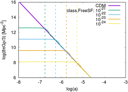
Figure 1. The background solution of the SFDM density, for different values of the boson mass m_a, in comparison with the case of CDM. The numerical solutions were obtained from the Boltzmann code CLASS.FreeSF that solves the polar form of the KG equation (2) discussed in section 2.1. The vertical dashed lines indicate the values of the scale factor a_osc at the start of the rapid oscillations of the scalar field ϕ; the values of a_osc were obtained from the equivalent solutions of the Boltzmann code axioncamb.

2.2. Linear Perturbations

The next step in the analysis is to find the behavior of linear perturbations and to verify that the scalar field DM allows the formation of structure following the standard CDM paradigm. Within the synchronous gauge of metric perturbations, in which the line element is written as $d{s}^2=-d{t}^2+a^2({\delta }_{ij}+{\bar{h}}_{ij})d{x}^{i}d{x}^j$, the linearly perturbed KG equation in Fourier space for a given wavenumber k reads:

$\begin{array}{ll}\ddot{\phi }=-3H\dot{\phi }-\left(\frac{k^2}{a^2}-m_a^2\right)\phi -\frac{1}{2}\dot{\varphi }\dot{\overline{h}},& (7)\end{array}$

where we are considering that ϕ(t, k) = ϕ(t)+φ(t, k), with φ a small field perturbation, and $\bar{h}={h^l}_l$ is the trace of the spatial perturbations in the metric. Reliable numerical simulations can be obtained if we define polar variables in the form:

$\begin{array}{ll}\kappa \dot{\phi }=-{\Omega }_{\varphi }^{1/2}{e}^{\alpha }\cos (\vartheta /2),\kappa m_a\phi =-{\Omega }_{\varphi }^{1/2}{e}^{\alpha }\sin (\vartheta /2),& (8)\end{array}$

where α and ϑ are the new dynamical variables. However, it is better to define new variables:

$\begin{array}{ll}{\delta }_0=\delta {\rho }_{\varphi }/{\rho }_{\varphi }=-e^{\alpha }\sin (\theta /2-\vartheta /2),{\delta }_1=-e^{\alpha }\cos (\theta /2-\vartheta /2),& (9)\end{array}$

under which the perturbed KG equation (7) is written also as a dynamical system (Ureña-López and Gonzalez-Morales, 2016; Cedeño et al., 2017):

$\begin{array}{l}\frac{d{\delta }_0}{d(\ln a)}=\left[-3\sin \theta -\frac{k^2}{k_J^2}(1-\cos \theta )\right]{\delta }_1+\frac{k^2}{k_J^2}\sin \theta {\delta }_0\\ -\frac{1}{2}\frac{d\overline{h}}{d(\ln a)}(1-\cos \theta ),& (\mathrm{10a})\end{array}$

$\begin{array}{l}\frac{d{\delta }_1}{d(\ln a)}=\left[-3\cos \theta -\frac{k^2}{k_J^2}\sin \theta \right]{\delta }_1+\frac{k^2}{k_J^2}\left(1+\cos \theta \right){\delta }_0\\ -\frac{1}{2}\frac{d\overline{h}}{d(\ln a)}\sin \theta ,& (\mathrm{10b})\end{array}$

where $k_J^2\equiv 2a^{2}H{m}_a$ is the (squared) Jeans wavenumber that naturally arises because of the wave nature of the scalar field.

The interesting regime, as before for the background dynamics in section 2.1, is that of rapid oscillations, under which Equation (10) become:

$\begin{array}{ll}\frac{d{\delta }_0}{d(\ln a)}=-\frac{k^2}{k_J^2}{\delta }_1-\frac{1}{2}\frac{d\overline{h}}{d(\ln a)},\frac{d{\delta }_1}{d(\ln a)}=\frac{k^2}{k_J^2}{\delta }_0.& (11)\end{array}$

For length scales k ≪ k_J, we recover the same expression as that of the density contrast for CDM, namely, ${\stackrel{\bullet }{\delta }}_0=-(1/2)\stackrel{\bullet }{\bar{h}}$, whereas δ₁ remains approximately constant. However, in the opposite regime k ≫ k_J, Equation (11) resemble that of a harmonic oscillator, and then the density perturbations cannot grow as much as those of CDM.

As before for the background, we show in Figure 2 the solutions of the linear density perturbations of SFDM in comparison with those of CDM, as obtained from the Boltzmann code CLASS and its amended version CLASS.FreeSF. In the case of the so-called mass power spectrum (MPS), we notice the sharp cut-off that has become a trademark of SFDM ever since it was firstly shown in Matos and Arturo Ureña-López (2001) as an output of the now outdated Boltzmann code CMBFast. We also show in the same plot the output from axioncamb, which seems to differ a little bit regarding the profile of the MPS at around the cut-off scale in the two cases shown ($m_a=10^{-22},10^{-24}\text{eV}$). The differences may indicate here some discrepancy in the treatment of linear perturbations in the two Boltzmann codes: CLASS.FreeSF directly solves the (polar) Equations (10), whereas axioncamb uses a formal equivalence of the field perturbations to those of a fluid, following the prescription in Hu (1998) and the scale-dependent speed of sound suggested in Hwang and Noh (2009). Moreover, we also show the analytic formula put forward in Hu et al. (2000) for the linear MPS. With the latter being just an analytic approximation without proper backup from a Boltzmann code, its manifest discrepancies with the aforementioned numerical results should not be surprising after all, and this little exercise suggests that it would be better to use the numerical output from the Boltzmann codes rather than the approximation to model the MPS.

FIGURE 2

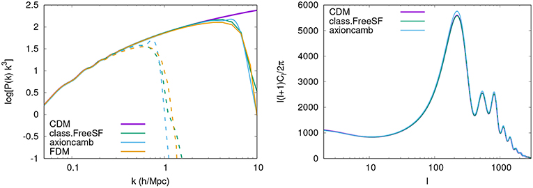
Figure 2. The MPS (Left) and the anisotropies of the CMB (Right) obtained for the SFDM model from the amended Boltzmann codes CLASS.FreeSF and axioncamb. As explained in section 2.2, the code CLASS.FreeSF solves the polar form of the perturbed KG equation (10), whereas axioncamb solves its equivalent fluid form. In general, SFDM looks indistinguishable from CDM, although there are some small discrepancies in the outputs generated by the Boltzmann codes.

In the case of the anisotropies of the Cosmic Microwave Background (CMB) the differences between the different models are almost unnoticeable, and then this observable is not able to distinguish SFDM from CDM, even if the boson mass changes in two orders of magnitude (recall that $m_a=10^{-22},10^{-24}\text{eV}$). However, the outputs from CLASS.FreeSF and axioncamb do not agree completely again, which seems to point out some possible inconsistencies between the polar and fluid approaches to the KG equation at the level of linear perturbations. A more thorough analysis of the differences of the two codes will be reported elsewhere.

3. Gravitational Configurations of SFDM

Ever since the seminal paper (Ruffini and Bonazzola, 1969), there has been much interest in the properties of the gravitational objects made of scalar fields, in both the relativistic and non-relativistic regimes, see the comprehensive reviews in Jetzer (1992), Schunck and Mielke (2008), and Liebling and Palenzuela (2017). Different approaches have been devised to find the general features of the gravitational collapsed objects within a cosmological context (Widrow and Kaiser, 1993; Woo and Chiueh, 2009; Schive et al., 2014a; Uhlemann et al., 2014; Veltmaat and Niemeyer, 2016; Edwards et al., 2018), where it has been verified that the non-linear process of structure formation in SFDM models proceeds as in CDM for large enough scales.

According to the detailed analysis made in Schive et al. (2014a), Schwabe et al. (2016), and Mocz et al. (2017a), the gravitationally bounded objects that one could identify with DM galaxy halos all have a common structure: one central soliton surrounded by a Navarro-Frenk-White-like envelope created by the interference of the Schrodinger wave functions. In terms of the standard nomenclature, the SFDM model belongs to the so-called non-cusp, or cored, types of DM models. Although not yet completely conclusive, there seems to be an increasing evidence in favor of cored DM models (Walker and Peñarrubia, 2011; Rodrigues et al., 2018), and then the non-cusp nature of SFDM objects remain one of the most promising features of the model.

Here we will make a quick review of the general features of the soliton structures that arise from SFDM models, using for this the so-called field and fluid approaches, in order to highlight their equivalences and differences and their use in cosmological and astrophysical settings.

3.1. The Field Approach

The field approach to the formation of structure within the SFDM paradigm refers to the solutions obtained from the Schrodinger-Poisson (SP) system, which is represented by the equations:

$\begin{array}{ll}i\hslash {\partial }_t\psi =-\frac{\hslash }{2m_a}{\nabla }^2\psi +\Phi \psi ,{\nabla }^2\Phi =4\pi G{m}_a^2|\psi {|}^2,& (12)\end{array}$

where ψ is the wave function that collectively represents the boson particles in their ground state, and Φ is the Newtonian gravitational potential. Notice that the latter is calculated from the mass density effectively defined through $\rho =m_a^2|\psi {|}^2$. For the purposes of simplicity, we do not include any self-interaction term in the SP system, which would then become the Gross-Pitaeevski-Poisson system. For a discussion of the latter and its general properties at cosmological and astrophysical scales (see Barranco and Bernal, 2011; Li et al., 2013; Diez-Tejedor et al., 2014).

The SP system possesses the following scaling symmetry:

$\begin{array}{ll}\left\{t,x,\psi ,\Phi \right\}\to \left\{{\lambda }^{-2}\widehat{t},{\lambda }^{-1}\widehat{x},{\lambda }^2\widehat{\psi },{\lambda }^2\widehat{\Phi }\right\},& (13)\end{array}$

for an arbitrary value of the scaling parameter λ. It is then common to choose a particular configuration and then find any others by a proper scaling of the different quantities to ease the numerical effort.

3.2. The Fluid Approach

There is also a fluid equivalent of the SP system (12), for which we only need to apply the so-called Madelung transformation of the wave function by means of ψ(t, x) = φ(t, x)exp(−iS(t, x)/ℏ). The resultant equations of motion are then:

$\begin{array}{ll}\dot{\phi }=\frac{1}{2}\phi {\nabla }^{2}S+\nabla \phi ·\nabla S,\phi \left[\dot{S}+\frac{1}{2}{(\nabla S)}^2+\Phi -\frac{1}{2}\frac{{\nabla }^2\phi }{\phi }\right]=0.& (14)\end{array}$

Notice, under the assumption that φ ≠ 0, that the scalar function S obeys a Hamilton-Jacobi type of equation Ṡ + H(∇S, x, t) = 0, in which the potential part in the Hamiltonian H is represented by two terms: Φ + Q, where Q is the so-called quantum potential:

$\begin{array}{ll}Q=-\frac{1}{2}\frac{{\nabla }^2\phi }{\phi }.& (15)\end{array}$

Taking the assumption φ ≠ 0 for granted, one can further manipulate Equation (14) to write them down as fluid equations. We define the velocity field v = − ∇ S and the mass density $\rho =m_a^2|\psi {|}^2=m_a^2{\phi }^2$, and then the SP system becomes the Quantum Euler-Poisson (QEP) system (for details see Wallstrom, 1994; Chavanis, 2011; Uhlemann et al., 2014).

$\begin{array}{l}\frac{\partial \rho }{\partial t}+\nabla ·(\rho v)=0,\frac{\partial v}{\partial t}+(v·\nabla )v=-\nabla \Phi -\nabla Q,\\ {\nabla }^2\Phi =4\pi G\rho .& (16)\end{array}$

Equation (16) are the standard fluid equations except for the presence of the quantum potential Q. The QEP also posses the same scaling symmetry of the SP system, namely:

$\begin{array}{ll}\left\{t,x,\rho ,S,v,\Phi ,Q\right\}\to \left\{{\text{λ}}^{-2}\widehat{t},{\text{λ}}^{-1}\widehat{x},{\text{λ}}^4\widehat{\rho },\widehat{S},\text{λ}\widehat{v},{\lambda }^2\widehat{\Phi },{\text{λ}}^2\widehat{Q}\right\}\text{}.& (17)\end{array}$

Notice that the function S is scale invariant, whereas the velocity field v is not.

3.3. Stationary Equilibrium Configurations

We call equilibrium configurations to those spherically symmetric solutions of the SP system (12) that arise from the ansatz ψ = φ(r)exp(−iγt) (Ruffini and Bonazzola, 1969; Guzmán and Ureña-López, 2004), and which are then solutions of the eigenvalue problem:

$\begin{array}{ll}{\nabla }^2\phi =2\left(\Phi -\gamma \right)\phi ,{\nabla }^2\Phi =4\pi G{\phi }^2.& (18)\end{array}$

Given the scaling symmetry of the SP system, one only has to find the solution corresponding to the special value φ(0) = 1 to determine the full family of solutions. Different numerical solutions, classified in terms of the number of nodes in the wavefunction, are shown in Figure 3.

FIGURE 3

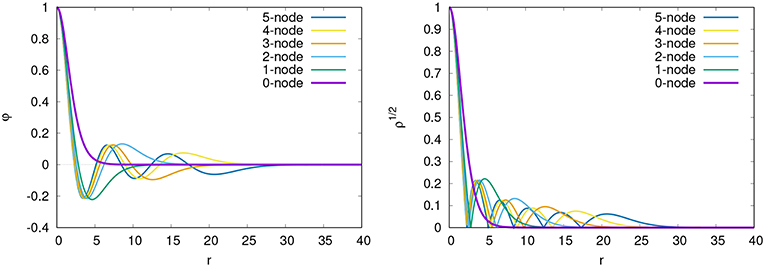
Figure 3. Different equilibrium solutions of the SP system (12), see also Equations (18): the amplitude of the wavefuction ψ(0, r) = φ(r) (Left) and the square root of the density ρ^1/2 = |ψ(r)| (Right). The ground state corresponds to the node-less wavefunction, see the text for more details.

From the fluid approach, equilibrium configurations arise from the conditions ρ(t, r) = ρ(r) and v = 0. The conservation equations are identically satisfied, whereas the Euler equation implies that ∇Φ = −∇Q (the quantum force acts against the gravitational one), and then one arrives to the Poisson equation in the form:

$\begin{array}{ll}{\nabla }^2\left(\frac{{\nabla }^2\sqrt{\rho }}{\sqrt{\rho }}\right)=8\pi G\rho .& (19)\end{array}$

In principle, one only needs to solve the cumbersome Equation (19) to find the equilibrium configuration in the Madelung representation of SFDM. It is not clear at first sight whether Equation (19) will lead us to an eigenvalue problem, unless one takes further assumptions by hand. For instance, from the equilibrium of forces one obtains Q = Φ+γ, where γ is a constant, and then Equation (19) could be rewritten in the same form as Equation (18) as long as we identify ρ = φ². However, one can see that this procedure is not as clean or as direct as the one from the original SP system. Moreover, for equilibrium configurations, the wavefunction, and in turn the density, has nodes, which means that there are points at which the quantum potential cannot be calculated directly from the expression Q = −(1/2)∇²φ/φ, simply because there will be a division by zero at the node points of the wavefunction φ. But the first of Equation (18) tells us that the ratio ∇²φ/φ = 2(Φ−γ) should be well behaved everywhere, although this can only be known in the field approach and not in the fluid one (see again Figure 3).

3.4. Shortcomings of the Fluid Approximation

Although the Madelung transformation compels us to believe in the equivalence between the field and fluid approaches for the gravitational collapse of SFDM objects, one has to bear in mind that such equivalence works, strictly speaking, in one direction only, namely, from the SP system to the QEP one. As it is convincingly described in Wallstrom (1994), the equivalence is not true in the opposite direction: one cannot recover a truthful wavefunction from the solution of the density ρ and velocity v fields. The main objection is that we cannot recover the quantum nature, or to be more conservative, the discrete nature of some physical quantities related to the SP system, without the introduction of extra constraints. More precisely, it is argued in Wallstrom (1994) that one may be required to impose the discretization condition ∮_Lv·dℓ = 2πj for any closed loop L and any integer j. The latter condition translates into ∮_LdS = Δ_LS = 2πj, with which one could recover a single-valued wavefunction ψ at any point in configuration space.

One then sees that the sensible point is the solution of the velocity field, or in turn the solution of the action function S, especially in the cases in which there is angular momentum or any non-spherically symmetric collapse. In Wallstrom (1994) the author mentions the case of axially-symmetric solutions for which S = mφ, with m an integer number and φ here the azimuthal angle. But one must remember that there is another quantum number which is the energy of the system and that is also related to the action function: E_n = ∂_tS. There is not for the latter case a quantization condition that one could impose upon the solutions of the QEP system as simple as the one described before (ΔS_L = 2πj).

Another important feature of the equilibrium configurations shown in section 3.3 is that the only stable one is the ground state, node-less, solution, which is also the attractor solution a general configuration settles down onto, a property that was comprehensively studied in Guzmán and Ureña-López (2004) and Guzmán and Avilez-Lopez (2018). That any arbitrary, initial, field configuration ψ evolves toward the ground state is a consequence of the appropriateness of the SP system to provide an eigenvalue solution by dynamical means. In other words, the eigenvalue solution ψ = φ(r)e^−iγt emerges eventually during the evolution of the field configuration. Such a property is seemingly non-existent in the fluid approach, and then one must be skeptical again of the equivalence between the two methods. So far, it has just been reported in Veltmaat and Niemeyer (2016) that the ground state remains stable in the two approaches, but it was not shown that the ground state is the attractor solution and that the QEP system (16) is able to find it together with the correct eigenvalues and eigenfunctions.

3.5. Energy Considerations of SFDM Gravitational Configurations

As explained in Guzmán and Ureña-López (2004), Guzmán and Ureña-López (2006), and Hui et al. (2017), there are some physical quantities that help us to monitor the evolution of the wavefunction, but given that we will be dealing with a single configuration here we will use the energy quantities, namely:

$\begin{array}{l}E={\displaystyle {\int }_V\text{Im}}({\psi }^{\ast }{\partial }_t\psi )d{V}^{\prime },K=-\frac{1}{2}{\displaystyle {\int }_V\text{Re}}({\psi }^{\ast }{\nabla }^2\psi )d{V}^{\prime },\\ W={\displaystyle {\int }_V\Phi }|\psi {|}^{2}d{V}^{\prime },& (20)\end{array}$

where E is the total energy, K is the kinetic energy and W the potential energy. Directly from the Schrodinger equation (12), one can show that the three quantities are related through E = K+W. In the case of equilibrium configurations one finds that E = (1/3)γM and K/|W| = 1/2, which means that the total energy is negative E < 0 and that the configuration is virialized, independently of the number of nodes in the (stationary) wavefunction φ.

All the above quantities can be rewritten in terms of the Madelung variables as:

$\begin{array}{l}E=-{\displaystyle {\int }_V{\partial }_t}S{\phi }^{2}d{V}^{\prime },K=-\frac{1}{2}{\displaystyle {\int }_V\left[\phi {\nabla }^2\phi -{\phi }^2{(\nabla S)}^2\right]}d{V}^{\prime },\\ W={\displaystyle {\int }_V\Phi }{\phi }^{2}d{V}^{\prime }.& (21)\end{array}$

Alternatively, in terms of the fluid equations, one finds:

$\begin{array}{l}K=K_Q+K_v=-\frac{1}{2}{\displaystyle {\int }_V\left(\frac{{\nabla }^2\sqrt{\rho }}{\sqrt{\rho }}\right)}\rho d{V}^{\prime }+\frac{1}{2}{\displaystyle {\int }_V\rho }{v}^{2}d{V}^{\prime },\\ W={\displaystyle {\int }_V\Phi }\rho d{V}^{\prime }.& (22)\end{array}$

It must be noticed that the kinetic energy K is composed of two terms, one related to the quantum potential Q and another one to the velocity field v. The virialization of the system, if it is going to coincide with the field expression, should be written as K/|W| = (K_Q+K_v)/|W| = 1/2, and not simply as K_v/|W| = 1/2, which would be the direct expression within the fluid approach. Actually, the latter expression would be completely wrong in the case of equilibrium configurations for which, as we have seen above, the kinetic energy due to the velocity dispersion of the fluid is K_v = 0.

The virial ratio K/|W| is indeed one important quantity in the evolution of gravitational configurations; such a ratio is 1/2 for virialized systems, and then we can say that a gravitational configuration is overwarmed (underwarmed) if K/|W|> 1/2 (K/|W| < 1/2). As reported in Seidel and Suen (1990), Guzmán and Ureña-López (2004), and Guzmán and Ureña-López (2006), a gravitational configuration can resort to the mechanism of gravitational cooling to get rid of the excess in the kinetic energy and eventually reach a virialized state. The cases studied in Guzmán and Ureña-López (2004) only considered reasonable values of the virial ratio, and for the largest value considered (K/|W|≃1.2, see Figure 18 in Guzmán and Ureña-López, 2004), the configuration had to expand for about 100 times its initial radius and expel about 90% of its initial mass before it could become an equilibrium configuration. This tells us about the role played by the virial ratio to determine how long, if at all, it would take for a given system to find a stationary configuration.

4. Cosmological Collapse of SFDM Cosmological Configurations

The whole process of structure formation, and its various implications, have been studied recently in dedicated numerical simulations. The majority of them rely on standard N-body codes but with modified initial conditions that reflect the properties of SFDM at the level of linear density perturbations in the mass power spectrum as obtained from the amended Boltzmann codes (Hlozek et al., 2015; Ureña-López and Gonzalez-Morales, 2016). However, there are some others that solve directly the SP system (Schive et al., 2014a; Mocz et al., 2017a; Edwards et al., 2018), which would be the most reliable ones, and also others that consider the equivalent fluid approach by means of the Madelung transformation of the wave function (Nori and Baldi, 2018; Zhang et al., 2018). In these latter codes the quantum pressure has to be approximated in its numerical implementation, and there is not yet conclusive proof that they deliver the same results as those of the SP system (although see Li et al., 2019).

4.1. The Top-Hat Model for SFDM

Many details are given in Guzmán and Ureña-López (2004) for the evolution of unstable configurations, and here I will only show one further example which would be equivalent to the top-hat model for the gravitational collapse of CDM (see also Siddhartha Guzmán and Arturo Ureña-Lòpez, 2003). For that, let us consider a spherical configuration with a constant density, which is equivalent to |ψ₀| = const., and total radius r_T. The total mass contained within the sphere is $M_T=(1/3)|{\psi }_0{|}^2{r}_T^3$, or in terms of dimensionless (ket) quantities we have $M_T={\widehat{M}}_T{m}_{\text{Pl}}^2/m$, with ${\widehat{M}}_T=(1/3)|{\widehat{\psi }}_0{|}^2{\widehat{r}}_T^3$. Likewise, the physical density is $\rho =|\widehat{\psi }{|}^2{m}_{\text{Pl}}^2{m}_{\psi }^2/(4\pi )$, whereas for the physical radius we have $r_T={\widehat{r}}_T/m$.

We further assume that the spherical configuration is about to collapse under its own gravity, i.e., it is about to separate from the general expansion of the universe at the time of turnaround. In terms of the fluid picture, this just means that the kinetic energy due to the dispersion velocity of the particles is null, K_v = 0. However, the potential part of the kinetic energy K_Q is still present, and we should take it into account in the energy calculations.

A back-of-the-envelope calculation, using Equation (20), can be used to estimate the order of magnitude expected for the virial ratio of the spherical configuration at turnaround. The gravitational potential is of the order of $\Phi ~-|{\widehat{\psi }}_0{|}^2{\widehat{r}}^2$, and then the gravitational energy in the configuration is $W~-|{\widehat{\psi }}_0{|}^4{\widehat{r}}_T^5$. In the same manner, the kinetic energy is given by $K~|{\widehat{\psi }}_0{|}^2{\widehat{r}}_T$, and then the virial ratio is of the order of $K/\left|W\right|~1/(|{\widehat{\psi }}_0{|}^2{\widehat{r}}_s^4)$. Of course, in the ideal case $\widehat{\psi }=\text{const}.$ the kinetic energy is exactly zero, but on more realistic grounds the wavefunction must have a profile a bit different from that of the step function and some extra contribution to the kinetic energy comes from its derivatives in the term K_Q. Thus, the estimation above about the virial ratio K/|W| should considered a lower bound on its true value². Notice that the quantity $|{\widehat{\psi }}_0{|}^2{\widehat{r}}_T^4$ is an invariant quantity according to the scaling transformation (13), and then it is truly representative of the system under study. Moreover, it cannot either be tailored to ease the numerical effort. This has a strong physical consequence for the evolution of the gravitational configuration, as we are going to show now.

For the purposes of illustration, let us consider that the constant density is the same as that of DM, $|{\psi }_0{|}^2=(3H_0^2/8\pi G){\Omega }_{b0}{a}^{-3}$, and that r_T is its comoving radius (the physical radius would be r_{T, phys} = ar_T). The physical density in terms of the field variables is $|{\psi }_0{|}^2=|{\widehat{\psi }}_0{|}^2{m}_{\text{Pl}}^2{m}_{\psi }^2/(4\pi )$, where ${\widehat{\psi }}_0$ is the dimensionless wavefunction. After a bit of algebra we find³:

$\begin{array}{ll}|{\widehat{\psi }}_0{|}^2=6.86\times {10}^{-22}\frac{h^2}{m_{a22}^2}{\Omega }_{M0}{a}^{-3},& (\mathrm{23a})\end{array}$

where H is the reduced Hubble constant and $m_{a22}=m_a/10^{-22}\text{eV}$. Likewise, the dimensionless radius would be given by ${\widehat{r}}_T=m_a{r}_T$. Then, from the definition of the total mass we find the following relation for the dimensionless quantities:

$\begin{array}{ll}|{\widehat{\psi }}_0{|}^2{\widehat{r}}_T^3=2.32\times {10}^{-12}{m}_{a22}(M_T/M_{\odot }){\Omega }_{M0}^{-1}.& (\mathrm{23b})\end{array}$

From the combination of the two equations (23), we finally find that

$\begin{array}{ll}|{\widehat{\psi }}_0{|}^2{\widehat{r}}_T^4=3.48\times {10}^{-9}{m}_{22}^2{h}^{-2/3}{\Omega }_{M0}^{-5/3}{\left(M_T/M_{\odot }\right)}^{4/3}a.& (24)\end{array}$

Equation (24) indicates that the virial ratio of the cosmological sphere of matter has a very clear dependence on the boson mass, the total mass and the scale factor, namely, $K/\left|W\right|~10^7{m}_{22}^{-2}{(M_T/M_{\odot })}^{-4/3}{a}^{-1}$ (with h = 0.67, Ω_M0 = 0.26). The condition K/|W|≲1 seems to suggest that configurations with masses $M_T\lesssim 10^5{M}_{\odot }{m}_{a22}^{-3/2}{a}^{-3/4}$ are overwarmed and most likely will be unable to collapse eventually into an equilibrium configuration. There is some weak dependence on the scale factor, and from it we can conclude that configurations with $M_T<10^5{M}_{\odot }{m}_{a22}^{-3/2}$ cannot collapse and form virialized objects. This prediction comes directly from the intrinsic properties of the cosmological setup, more specifically from the (dimensionless) values of the density $|{\widehat{\psi }}_0{|}^2$ and total radius ${\widehat{r}}_T$ that are needed to achieve the cosmological masses annotated above, and it is of general applicability for any particular profile of the mass density at the time of turnaround.

The existence of a lower mass for the gravitational collapse has been inferred before from the evolution of linear density perturbations (see section 2.2 above), but our calculations here show that such cut-off mass scale should also appear naturally from the evolution of the SP system if the initial configuration complies with the cosmological values. In our estimation, the virial ratio also has a clear dependence on the boson mass, $K/\left|W\right|\propto m_{a22}^{-2}$, which implies that less massive configurations can collapse into equilibrium configurations for larger values m_a22 ≫ 1. Actually, all mass values M_T are allowed to collapse gravitationally, however small they are, in the limit m_a22 → ∞, in which the SFDM model becomes indistinguishable from the CDM model.

4.2. Relativistic Effects

In general, the total mass of stable, self-gravitating configurations in SFDM models is given as $M_T=\beta (m_{\text{Pl}}^2/m)$, where β≲0.6. This indicates that there is a maximum mass for stability: configurations with a larger value can either migrate to a stable configuration or collapse into black holes, see the works in Seidel and Suen (1990, 1991) and Alcubierre et al. (2003). Moreover, according to the studies in Guzmán and Ureña-López (2004), the SP system is a good approximation to the EKG one under the condition that β ≲ 0.02, because for larger values one has to take into account relativistic effects for a proper gravitational evolution of the system. For instance, for a sufficiently massive configuration with β ≳ 1, the SP system predicts its collapse into a very dense, small but regular object, whereas the EKG system would predict the formation of a black hole. In our case we see that the mass parameter is $\beta \simeq (1/3)|{\psi }_0{|}^2{\widehat{r}}_T^3$, and from the values calculated from Equation (23b), we must conclude that the SP system (12) cannot follow reliably the gravitational collapse of systems with masses $M_T\gtrsim 10^{11}{M}_{\odot }$.

5. Universal Soliton Profile

One of the most remarkable features of the gravitational structures found in the simulations of SFDM (Schive et al., 2014a; Mocz et al., 2018) is the presence of a soliton core in all of them, which is surrounded by an interference pattern that resembles the so-called Navarro-Frenk-White profile that is typical in N-body simulations of CDM. The soliton core is an unavoidable result of the wave nature of the boson particles within the SFDM paradigm, and its properties can be understood from those of the equilibrium configurations of the SP system (see section 3.3). Some properties of the soliton configurations are discussed next in connection with some galaxy data.

5.1. Soliton Profile in Satellite Galaxies

There has been some recent interest in the possibility to detect the presence of soliton core in different galaxies. Satellite galaxies are the obvious candidates to search for intrinsic scale properties of DM, in particular for any central structure like a soliton. So far, studies with a Jeans analysis suggest that the boson mass should be m_a22 ≲ 0.1 (Diez-Tejedor et al., 2014; Marsh and Silk, 2014; Lora, 2015; Gonzalez-Morales et al., 2016; Ureña-López et al., 2017; Bar et al., 2018; De Martino et al., 2018). Here we will do a simple exercise to make a comparison with some galaxy data, and for that we will propose a new observable that takes into account the scaling properties of the SP system (13).

Let us consider the density profile of SFDM solitons ρ(r) as characterized by the semi-analytic approach in Marsh (2015a):

$\begin{array}{ll}\rho (r)=\frac{{\rho }_s}{{(1+r^2/r_s^2)}^8},& (25)\end{array}$

where ρ_s is the central density and r_s is the scale radius. The parameters ρ_s and r_s are predicted to have the following scaling property: ${\rho }_s={\lambda }^4{m}_a^2{m}_{\text{Pl}}^2/4\pi$ and $r_s={(0.23\lambda m_a)}^{-1}$, where m_Pl is the Planck mass, m_a is the mass of the boson particle and λ is the scaling parameter in Equation (13). It is shown in Figure 4 that Equation (25) is a good approximation of the numerical result up to r = r_s. Likewise, the mass M_s of the soliton profile can be obtained from:

$\begin{array}{l}{M}_s(r)=4\pi {\rho }_s{r}_s^3{\widehat{M}}_s(r/r_s)=\frac{\lambda }{{(0.23)}^3}\frac{m_{\text{Pl}}^2}{m_a}{\widehat{M}}_s(r/r_s),\\ {\widehat{M}}_s(r/r_s)={\displaystyle {\int }_0^{r/r_s}\frac{x^{2}dx}{{(1+x^2)}^8}}.& (26)\end{array}$

The total mass of the configuration is obtained when r → ∞, and then $M_s=2.08\lambda (m_{\text{Pl}}^2/m_a)$, which is in agreement with previous results (Guzmán and Ureña-López, 2004). It can be shown that the radius containing 95% of the total mass is r₉₅≃0.89r_s, and then as a rule of thumb we can say that the scale radius is a good measure of the total radius of the whole configuration.

FIGURE 4

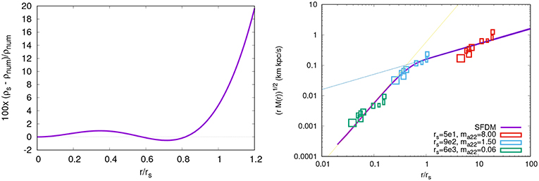
Figure 4. (Left) Comparison between the numerical (see section 3.3) and semianalytical (see Equation 25) profiles of the density ρ = |ψ|² in the case of a stationary equilibrium configuration. Notice that the relative error between the two cases is less than 4% up to r = r_s. At larger distances the difference grows enormously because the numerical profile decays exponentially. (Right) The observable quantity [rM(r)]^1/2, see Equation (27), calculated from the corresponding quantities reported in Fattahi et al. (2016) of the eight classical Milky Way dwarf spheroidals. The observable is scale invariant, see Equation (13), but the colors of the error boxes indicate the corresponding different values of the boson mass m_a and the soliton radius r_s. The magenta curve represents the complete profile of the observable, whereas the yellow and cyan straight lines indicate the asymptotic behaviors at small (~r²) and large radii (~r^1/2), respectively.

Given the scaling properties of the different quantities, it can be seen that a good observable is the quantity:

$\begin{array}{ll}{\left[G{M}_s(r)r\right]}^{1/2}=\frac{121}{m_{a22}}{\left[{\widehat{M}}_s(\widehat{r})\widehat{r}\right]}^{1/2}\text{km kpc }{\text{s}}^{-\text{1}},& (27)\end{array}$

where M_s(r) is the enclosed mass at radius r and $\widehat{r}=r/r_s$. The combination M_s(r)r does not depend on the scaling parameter λ, but only on the boson mass. The enclosed mass at a given radius can be estimated in different galaxies, and from them we could make an estimation of the presence of a soliton center using the new observable (27).

Considering the data of the classical satellites in the Milky Way from Fattahi et al. (2016), we show in Figure 4 a comparison with the theoretical profile that corresponds to an equilibrium configuration. There are two free parameters: m_a22 and r_s, and then one only has to adjust them to get a fit to the theoretical curve (in doing so, we are implicitly adjusting the scaling parameter too, see Equation 25). In the plot we considered three different combinations of the parameters (m_a22, r_s), which are indicated by the corresponding colors. The best fit-by-eye seems to be the intermediate case with m_a22 = 1.5 and r_s = 900pc, that somehow follows the transition trend of the soliton configuration at r≃r_s. This would mean that the size of the DM halo in the satellites seem to agree with that of a single soliton, with a total mass of about $10^8{M}_{\odot }$, which would be in agreement with previous estimations of the mass contained in the Milky Way satellites (Strigari et al., 2008). However, notice that the comparison is not conclusive, as the data boxes for lower boson masses m_a22 are not completely out of fit, which could explain that some of the detailed studies so far can only put an upper bound m_a22 ≲ 0.1 (Marsh, 2015a; Gonzalez-Morales et al., 2016; Bernal et al., 2017).

5.2. The Core-Halo Relation and Galaxy Data

The presence of a soliton in the center of larger galaxies is more difficult to detect. For instance, in De Martino et al. (2018) the authors tried to disentangle the contributions to the rotation curve of different matter components in the central parts of the Milky Way. They determine that, within the error bars in the observational data, there seems to be strong enough evidence for the presence of a soliton with parameters.

A similar study was done in Bar et al. (2018) but for a larger sample of galaxies. Quite interestingly, the study takes into account theoretical constraints that can be inferred from the numerical simulations of the SP system (Schive et al., 2014a), and put them under scrutiny given the galaxy data. One main assumption is the so-called core-halo relation found in the simulations, and which is summarized in the expression $M_c\propto M_h^{1/3}$, where M_c (M_h) is the core (halo) mass. It is shown in Bar et al. (2018) that the core-halo relation suggests another one (see their Equation 35): that the specific energy for the central soliton and the host halo are the same, in other words:

$\begin{array}{ll}{\frac{E}{M}|}_{\text{soliton}}\simeq {\frac{E}{M}|}_{\text{halo}}.& (\mathrm{28a})\end{array}$

This interesting relation is arguably inferred from the properties of the halo profiles found in the dedicated numerical simulations in Schive et al. (2014a,b), which, as we mentioned before, are the only ones that solve directly the SP system within a cosmological context. Equation (28) is quite interesting, as the number on its lhs can be readily calculated from the properties of the equilibrium configurations discussed in section 3.3. According to the calculations in Guzmán and Ureña-López (2004) and Bar et al. (2018), we find that $E/M{|}_{\text{soliton}}=(1/3)\gamma =(1/3){\lambda }^2\widehat{\gamma }$, where $\widehat{\gamma }=-0.69$ is the (dimensionless) characteristic frequency of the soliton configurations (which have also been identified in simulations, e.g., Mocz et al., 2017b), and λ is the scaling parameter in Equation (13).

That the energy per unit mass is the same seems to be counterintuitive at first sight: for the soliton, it corresponds to its gravitational equilibrium (the eigenvalue problem explained in section 3.3), whereas there is not such a case for the host halo, at least not one that could be expected from first principles. As explained in Schive et al. (2014b) (see their Figure 3), the final configuration seems to consist of a central soliton surrounded by density granules that appear from the quantum interference of the wavefunction and which seem to be of the same size as the soliton itself. In other words, the host halo appears from a very different physical process to that of the soliton configuration, which adds to the mystery of Equation (28a).

In a follow up paper, the authors of Bar et al. (2018) consider a wider sample of rotation curves but now consider that a better energy relation between the soliton and the host halo is given in terms of their kinetic energy (Bar et al., 2019), namely:

$\begin{array}{ll}{\frac{K}{M}|}_{\text{soliton}}\simeq {\frac{K}{M}|}_{\text{halo}}.& (\mathrm{28b})\end{array}$

As in the case of Equation (28a), we can give the exact expression for the soliton only, which is Guzmán and Ureña-López (2004): K/M|_soliton = −E/M|_halo = −(1/3)γ, given that the soliton configuration satisfies the virial relation K/|W| = 1/2, see section 3.5 above. Notice that for the soliton, whether we consider the total energy or just the kinetic one, the energy for unit mass is numerically the same, except for a change in sign. Again, that the numerical ratios seem to be the same for the two systems (soliton and halo) is not at all expected beforehand.

The discussion about the energy relations (28) is not trivial, as one prediction of particular importance is that, under the SFDM hypothesis, the peak rotation velocity in the interior parts of galaxies should match the one at its outer parts (Bar et al., 2018, 2019). The internal peak must be attributed to the soliton configuration, whereas the asymptotic value comes from the NFW envelope, if the matching of the two profiles is done consistently. According to the results reported in Bar et al. (2018), the presence of the internal soliton is not supported by the data and the latter put a lower bound on the fiel mass of m_a22> 10, which is inconsistent with other studies (see section 5.1 above) ⁴.

5.3. Multi-State Configurations

It must be clear that the topic of the core-halo relations is not yet closed. For instance, in Mocz et al. (2017b) it is suggested that $M_{\text{soliton}}\propto |E{|}^{1/3}$, but as shown in Bar et al. (2018) this relation comes directly from the intrinsic scaling relation of the SP system (13). Moreover, in a more recent study in Chan et al. (2018), which even considers the contribution of stars in the simulations, it is found that resultant halos satisfy the expected scaling relations and that the granules that made up the halo are about the same size as the central soliton. Granules are a recurrent feature in cosmological simulations, and it seems that their presumed presence in galaxy halos is yet to be considered carefully in the comparison with galaxy data.

A related idea that was first proposed in Matos and Ureña-López (2007) is the gravitational co-existence of different energy eigenstates of the wavefunction; the resultant objects were called multi-state configurations. The idea behind this is that the ground state configuration, being the only one which is alone stable, can provide gravitational support for other excited states to also become stable (Ureña-López and Bernal, 2010), see also (Lin et al., 2018) for a similar approach. Actually, multi-state configurations are stable and virialized (just like the soliton-halo systems represented by Equation 28), as shown in Ureña-López and Bernal (2010) and Bernal et al. (2010) for both the non-relativistic and relativistic regimes, respectively. In this manner, one could build up complex configurations with a given number of ripples that could resemble the presence of granules in the simulations in Schive et al. (2014a), but further research is necessary before we can give solid evidence about this idea.

6. Conclusions

We have made a concise account of the properties of SFDM, in which the DM particle is described by a minimally coupled scalar field. If true, this model implies that DM is made up of ultra-light bosons whose quantum properties are able to show up at cosmological and astrophysical scales. Different observations seem to indicate that most likely the boson mass is of the order of 10⁻²²eV, which at the same time allows the model to comprise the totality of the DM budget and to explain the seemingly cored density profile in the central parts of the galaxies. However, it is not yet clear whether the SFDM model is to survive further tests, especially those at small scales that are most sensitive to the value of the boson mass and that are currently inconclusive about the preferred value of the boson mass.

To describe the non-linear process for the formation of structure within the SFDM paradigm, N-body simulations have been adapted to simulate the fluid description of the model, but they cannot yet capture the full field dynamics and the best option remains to solve directly the so-called Schrodinger-Poisson system. We have discussed the shortcomings of the fluid description in the simplest case possible represented by stationary equilibrium configurations. There is a reasonable doubt that the well-know solutions of the SP system for self-gravitating configurations can be faithfully replicated by the classical fluid equations, which casts further doubts in the results obtained from N-body emulators of the SFDM model. This is particulary acute in the cases in numerical simulations that only consider a cut-off in the MPS without taking into account the repulsive quantum force (see for instance Leo et al., 2018). As an example, we have studied a top-hat collapse model for SFDM, and found that the formation of low-mass systems could be prevented by the cosmological settings themselves because of the intrinsic wave nature of the equations of motion. More detailed studies are necessary to establish this newly found non-linear suppression of structure, and whether it is also present in the outputs from the N-body emulators.

Another remarkable prediction of the SFDM model is the presence of a soliton structure in the center of all galaxies, and this begs the question of the possible interaction of the boson particles with the supermassive black holes (SMBHs) that are reported to exist in the center of many galaxies. The masses of these SMBHs are in the range $10^4-10^6{M}_{\odot }$, quite similar to the estimated $10^7-10^8{M}_{\odot }$ of the aforementioned soliton cores. Preliminary studies indicate a non-trivial interaction between black holes and scalar fields (Ureña-López and Liddle, 2002; Barranco and Bernal, 2011; Brito et al., 2017; Avilez et al., 2018), but so far it seems that there is not a significant absorption of the field for the values of the boson mass in the range 10⁻²²−10⁻²¹eV, which are precisely of the most interest in cosmology and astrophysics.

One last topic that would have deserved a separate discussion is that about constraints arising from the comparison with observations of the Lyman-α forest, that so far seem to be the tightest ones according to recent studies (Armengaud et al., 2017; Iršič et al., 2017; Leong et al., 2019; Nori et al., 2019). These studies require results from dedicated N-body simulations with gas and stars, which seem to point out that the boson mass $m_a>10^{-21}\text{eV}$, and then there could be some incompatibility with the constraints obtained at astrophysical scales (except for the studies in Bar et al., 2018, 2019). However, given the current concerns about the reliability of the N-body emulators (Li et al., 2019), it seems wise to wait until further developments of the numerical codes allow a better interpretation of the Lyman-α forest within the SFDM paradigm.

Author Contributions

LU-L contributed to the analysis of the results presented and reviewed, and to the writing of the manuscript.

Funding

This work was partially supported by the Programa para el Desarrollo Profesional Docente, Dirección de Apoyo a la Investigación y al Posgrado, Universidad de Guanajuato, research Grants no. 206/2018-010/2019, CONACyT México under Grants No. 179881, No. 269652, No. A1-S-17899, No. 286897, and Fronteras 281, and the Fundación Marcos Moshinsky.

Conflict of Interest Statement

The author declares that the research was conducted in the absence of any commercial or financial relationships that could be construed as a potential conflict of interest.

Acknowledgments

I am grateful to Francisco Guzmán for his permission to use the numerical code of Ref. (Guzmán and Ureña-López, 2004) to generate some of the figures in this manuscript.

Footnotes

1. ^A separate kind of model exists in which all DM effects are attributed to a modification of gravity laws. The most famous exponent of such models is Modified Newtonian Dynamics (Milgrom, 1983, 2016). However, these models do not have a clear relativistic counterpart, and when they do their predictions are not in agreement with observational data. The most recent and stringent constraints come from the recent detection of gravitational waves, see for instance (Kahya and Woodard, 2007; Boran et al., 2018), which seems to rule out most such DM emulators.

2. ^For instance, for the initial configuration chosen in this section the kinetic energy is of the form $K~|{\widehat{\psi }}_0{|}^2{\widehat{r}}_s^3/{\Delta }^2$, where Δ would be the length scale for the variation of the derivatives. If our choice were Δ = r_T/10, the virial ratio should rather be $K/\left|W\right|~10^2/(|{\widehat{\psi }}_0{|}^2{\widehat{r}}_T^4)$. This is why the estimation used in the text should be considered a conservative lower bound.

3. ^In writing Equations (23) and (24), we have made use of the following relations in natural units for the boson mass: $m=1.56\times 10^7{m}_{a22}\text{Mp}{\text{c}}^{-1}=1.59\times 10^{-7}{m}_{a22}{\text{s}}^{-1}=4.79m_{a22}\text{y}{\text{r}}^{-1}=8.96\times 10^{-89}{m}_{a22}{M}_{\odot }$.

4. ^Another possibility to test the presence of a soliton configuration in the central parts of galaxies is to study its characteristic oscillations and their influence in the motion of stars. The first attempt in Marsh and Niemeyer (2018) considered the quasinormal frequency γ. However, a more complete study should also consider other higher frequencies, see (Guzmán, 2019). This is an interesting test that deserves further investigation.

References

Alcubierre, M., Becerril, R., and Guzm, F. S. (2003). Numerical studies of Phi 2 -oscillatons. Class. Quant. Gravity 20, 2883–2903. doi: 10.1088/0264-9381/20/13/332

CrossRef Full Text | Google Scholar

Arbey, A., Lesgourgues, J., and Salati, P. (2001a). Cosmological constraints on quintessential halos. Phys. Rev. D 65:083514. doi: 10.1103/physrevd.65.083514

CrossRef Full Text | Google Scholar

Arbey, A., Lesgourgues, J., and Salati, P. (2001b). Quintessential haloes around galaxies. Phys. Rev. D 64:123528. doi: 10.1103/physrevd.64.123528

CrossRef Full Text | Google Scholar

Arbey, A., Lesgourgues, J., and Salati, P. (2003). Galactic halos of fluid dark matter. Phys. Rev. D 68:023511. doi: 10.1103/physrevd.68.023511

CrossRef Full Text | Google Scholar

Armengaud, E., Palanque-Delabrouille, N., Yèche, C., Marsh, D. J. E., and Baur, J. (2017). Constraining the mass of light bosonic dark matter using SDSS Lyman-alpha forest. Mon. Notices R. Astron. Soc. 471, 4606–4614. doi: 10.1093/mnras/stx1870

CrossRef Full Text | Google Scholar

Avilez, A. A., Bernal, T., Padilla, L. E., and Matos, T. (2018). On the possibility that ultra-light boson haloes host and form supermassive black holes. Mon. Notices R. Astron. Soc. 477, 3257–3272. doi: 10.1093/mnras/sty572

CrossRef Full Text | Google Scholar

Bar, N., Blas, D., Blum, K., and Sibiryakov, S. (2018). Galactic rotation curves versus ultralight dark matter: implications of the soliton-host halo relation. Phys. Rev. D 98:083027. doi: 10.1103/PhysRevD.98.083027

CrossRef Full Text | Google Scholar

Bar, N., Blum, K., Eby, J., and Sato, R. (2019). Ultralight dark matter in disk galaxies. Phys. Rev. D 99:103020. doi: 10.1103/PhysRevD.99.103020

CrossRef Full Text | Google Scholar

Barranco, J., and Bernal, A. (2011). Self-gravitating system made of axions. Phys. Rev. D Part. Fields Grav. Cosmol. 83:043525. doi: 10.1103/PhysRevD.83.043525

CrossRef Full Text | Google Scholar

Bernal, A., Barranco, J., Alic, D., and Palenzuela, C. (2010). Multistate boson stars. Phys. Rev. D 81:044031. doi: 10.1103/PhysRevD.81.044031

CrossRef Full Text | Google Scholar

Bernal, T., Fernández-Hernández, L. M., Matos, T., and Rodríguez-Meza, M. A. (2017). Rotation curves of high-resolution LSB and SPARC galaxies with fuzzy and multistate (ultra-light boson) scalar field dark matter. Mon. Notices R. Astron. Soc. 475, 1447–1468. doi: 10.1093/mnras/stx3208

CrossRef Full Text | Google Scholar

Bertone, G., and Hooper, D. (2018). History of dark matter. Rev. Mod. Phys. 90:045002. doi: 10.1103/RevModPhys.90.045002

CrossRef Full Text | Google Scholar

Boran, S., Desai, S., Kahya, E. O., and Woodard, R. P. (2018). GW170817 falsifies dark matter emulators. Phys. Rev. D 97:041501. doi: 10.1103/PhysRevD.97.041501

CrossRef Full Text | Google Scholar

Brito, R., Ghosh, S., Barausse, E., Berti, E., Cardoso, V., Dvorkin, I., et al. (2017). Stochastic and resolvable gravitational waves from ultralight bosons. Phys. Rev. Lett. 119:131101. doi: 10.1103/PhysRevLett.119.131101

PubMed Abstract | CrossRef Full Text | Google Scholar

Cedeño, F. X., González-Morales, A. X., and Ureña-López, L. A. (2017). Cosmological signatures of ultralight dark matter with an axionlike potential. Phys. Rev. D 96, 1–6. doi: 10.1103/PhysRevD.96.061301

CrossRef Full Text | Google Scholar

Chan, J. H. H., Schive, H.-Y., Woo, T.-P., and Chiueh, T. (2018). How do stars affect ψDM haloes? Mon. Notices R. Astron. Soc. 478, 2686–2699. doi: 10.1093/mnras/sty900

CrossRef Full Text | Google Scholar

Chavanis, P.-H. (2011). BEC dark matter, Zeldovich approximation and generalized Burgers equation. Phys. Rev. D 84:063518. doi: 10.1103/PhysRevD.84.063518

CrossRef Full Text | Google Scholar

De Martino, I., Broadhurst, T., Tye, S. -H. H., Chiueh, T., and Schive, H.-Y. (2018). Dynamical evidence of a solitonic core of 10${}^9{M}_{\odot }$ in the milky way. arXiv:1807.08153.

Google Scholar

Diez-Tejedor, A., Gonzalez-Morales, A. X., and Profumo, S. (2014). Dwarf spheroidal galaxies and Bose-Einstein condensate dark matter. Phys. Rev. D 90:043517. doi: 10.1103/PhysRevD.90.043517

CrossRef Full Text | Google Scholar

Edwards, F., Kendall, E., Hotchkiss, S., and Easther, R. (2018). PyUltraLight: a pseudo-spectral solver for ultralight dark matter dynamics. J. Cosmol. Astro. Phys. 10:27. doi: 10.1088/1475-7516/2018/10/027

CrossRef Full Text | Google Scholar

Fattahi, A., Navarro, J. F., Sawala, T., Frenk, C. S., Sales, L. V., Oman, K., et al. (2016). The cold dark matter content of galactic dwarf spheroidals: no cores, no failures, no problem. arXiv:1607.06479.

Google Scholar

Gonzalez-Morales, A. X., Marsh, D. J. E., Peñarrubia, J., and Ureña-López, L. A. (2016). Unbiased constraints on ultralight axion mass from dwarf spheroidal galaxies. Mon. Notices R. Astron. Soc. 472, 1346–1360. doi: 10.1093/mnras/stx1941

CrossRef Full Text | Google Scholar

Guzmán, F. S. (2019). Oscillation modes of ultralight BEC dark matter cores. Phys. Rev. D 99:083513. doi: 10.1103/PhysRevD.99.083513

CrossRef Full Text | Google Scholar

Guzmán, F. S., and Avilez-Lopez, A. (2018). Head-on collision of multi-state ultralight BEC dark matter configurations. Phys. Rev. D 97:116003. doi: 10.1103/PhysRevD.97.116003

CrossRef Full Text | Google Scholar

Guzmán, F. S., and Ureña-López, L. A. (2004). Evolution of the Schrödinger-Newton system for a self-gravitating scalar field. Phys. Rev. D 69:124033. doi: 10.1103/PhysRevD.69.124033

CrossRef Full Text | Google Scholar

Guzmán, F. S., and Ureña-López,, L. A. (2006). Gravitational cooling of self-gravitating Bose-Condensates. Astrophys. J. 645, 814–819. doi: 10.1086/504508

CrossRef Full Text | Google Scholar

Hlozek, R., Grin, D., Marsh, D. J., and Ferreira, P. G. (2015). A search for ultralight axions using precision cosmological data. Phys. Rev. D 91:103512. doi: 10.1103/PhysRevD.91.103512

CrossRef Full Text | Google Scholar

Hooper, D. (2017). The relentless hunt for dark matter. Physics 10:119. doi: 10.1103/Physics.10.119

CrossRef Full Text | Google Scholar

Hu, W. (1998). Structure formation with generalized dark matter. Astrophys. J. 506, 485–494. doi: 10.1086/306274

CrossRef Full Text | Google Scholar

Hu, W., Barkana, R., and Gruzinov, A. (2000). Fuzzy cold dark matter: the wave properties of ultralight particles. Phys. Rev. Lett. 85, 1158–1161. doi: 10.1103/PhysRevLett.85.1158

PubMed Abstract | CrossRef Full Text | Google Scholar

Hui, L., Ostriker, J. P., Tremaine, S., and Witten, E. (2017). Ultralight scalars as cosmological dark matter. Phys. Rev. D 95:043541. doi: 10.1103/PhysRevD.95.043541

CrossRef Full Text | Google Scholar

Hwang, J.-C., and Noh, H. (2009). Axion as a cold dark matter candidate. Phys. Lett. B 680, 1–3. doi: 10.1016/j.physletb.2009.08.031

CrossRef Full Text | Google Scholar

Iršič, V., Viel, M., Haehnelt, M. G., Bolton, J. S., and Becker, G. D. (2017). First constraints on fuzzy dark matter from Lyman- α forest data and hydrodynamical simulations. Phys. Rev. Lett. 119:031302. doi: 10.1103/PhysRevLett.119.031302

PubMed Abstract | CrossRef Full Text | Google Scholar

Jetzer, P. (1992). Boson stars. Phys. Rep. 220, 163–227. doi: 10.1016/0370-1573(92)90123-H

CrossRef Full Text | Google Scholar

Ji, S. U., and Sin, S. J. (1994). Late-time phase transition and the galactic halo as a Bose liquid. II. The effect of visible matter. Phys. Rev. D 50, 3655–3659. doi: 10.1103/PhysRevD.50.3655

PubMed Abstract | CrossRef Full Text | Google Scholar

Kahya, E., and Woodard, R. (2007). A generic test of modified gravity models which emulate dark matter. Phys. Lett. B 652, 213–216. doi: 10.1016/j.physletb.2007.07.029

CrossRef Full Text | Google Scholar

Lee, J.-W. (2018). Brief history of ultra-light scalar dark matter models. EPJ Web Confer. 168:06005. doi: 10.1051/epjconf/201816806005

CrossRef Full Text | Google Scholar

Leo, M., Baugh, C. M., Li, B., and Pascoli, S. (2018). Nonlinear growth of structure in cosmologies with damped matter fluctuations. J. Cosmol. Astro. Phys. 1808:1. doi: 10.1088/1475-7516/2018/08/001

CrossRef Full Text | Google Scholar

Leong, K.-H., Schive, H.-Y., Zhang, U.-H., and Chiueh, T. (2019). Testing extreme-axion wave-like dark matter using the BOSS Lyman-alpha forest data. Mon. Not. Roy. Astron. Soc. 484, 4273–4286. doi: 10.1093/mnras/stz271

CrossRef Full Text | Google Scholar

Li, B., Rindler-Daller, T., and Shapiro, P. R. (2013). Cosmological constraints on Bose-Einstein-condensed scalar field dark matter. Phys. Rev. D 89:083536. doi: 10.1103/PhysRevD.89.083536

CrossRef Full Text | Google Scholar

Li, X., Hui, L., and Bryan, G. L. (2019). Numerical and perturbative computations of the fuzzy dark matter model. Phys. Rev. D 99:D63509. doi: 10.1103/PhysRevD.99.063509

CrossRef Full Text | Google Scholar

Liebling, S. L., and Palenzuela, C. (2017). Dynamical boson stars. Living Rev. Relativ. 20:5. doi: 10.1007/s41114-017-0007-y

PubMed Abstract | CrossRef Full Text | Google Scholar

Lin, S.-C., Schive, H.-Y., Wong, S.-K., and Chiueh, T. (2018). Self-consistent construction of virialized wave dark matter halos. Phys. Rev. D 97:103523. doi: 10.1103/PhysRevD.97.103523

CrossRef Full Text | Google Scholar

Lora, V. (2015). A universal SFDM Halo mass for the andromeda and milky Way'S Dsphs? Astrophys. J. 807:116. doi: 10.1088/0004-637X/807/2/116

CrossRef Full Text | Google Scholar

Magaña, J., Matos, T., Robles, V., and Suárez, A. (2012a). A brief Review of the Scalar Field Dark Matter model. J. Phys. Confer. Ser. 378:012012. doi: 10.1088/1742-6596/378/1/012012

CrossRef Full Text | Google Scholar

Magaña, J., Matos, T., Suárez, A., and Sánchez-Salcedo, F. J. (2012b). Structure formation with scalar field dark matter: the field approach. J. Cosmol. Astropart. Phys. 2012:003. doi: 10.1088/1475-7516/2012/10/003

CrossRef Full Text | Google Scholar

Marsh, D. J. (2015a). Nonlinear hydrodynamics of axion dark matter: relative velocity effects and quantum forces. Phys. Rev. D 91:123520. doi: 10.1103/PhysRevD.91.123520

CrossRef Full Text | Google Scholar

Marsh, D. J. E. (2015b). Axion cosmology. Phys. Rep. 643, 1–79. doi: 10.1016/j.physrep.2016.06.005

CrossRef Full Text | Google Scholar

Marsh, D. J. E., and Niemeyer, J. C. (2018). Strong constraints on fuzzy dark matter from ultrafaint dwarf galaxy Eridanus II. arXiv:1810.08543.

Google Scholar

Marsh, D. J. E., and Silk, J. (2014). A model for halo formation with axion mixed dark matter. Mon. Notices R. Astron. Soc. 437, 2652–2663. doi: 10.1093/mnras/stt2079

CrossRef Full Text | Google Scholar

Matos, T., and Arturo Ureña-López, L. (2001). Further analysis of a cosmological model with quintessence and scalar dark matter. Phys. Rev. D 63:063506. doi: 10.1103/PhysRevD.63.063506

CrossRef Full Text | Google Scholar

Matos, T., Guzmán, F. S., and Ureña-López, L. A. (2000). Scalar field as dark matter in the universe. Class. Quant. Gravity 17, 1707–1712. doi: 10.1088/0264-9381/17/7/309

CrossRef Full Text | Google Scholar

Matos, T., and Ureña-López, L. A. (2000). Quintessence and scalar dark matter in the universe. Class. Quant. Grav. 17, L75–L81. doi: 10.1088/0264-9381/17/13/101

CrossRef Full Text | Google Scholar

Matos, T., and Ureña-López, L. A. (2004). On the nature of dark matter. Int. J. Mod. Phys. D 13, 2287–2291. doi: 10.1142/S0218271804006346

CrossRef Full Text | Google Scholar

Matos, T., and Ureña-López, L. A. (2007). Flat rotation curves in scalar field galaxy halos. Gen. Relativ. Gravit. 39, 1279–1286. doi: 10.1007/s10714-007-0470-y

CrossRef Full Text | Google Scholar

Milgrom, M. (1983). A modification of the newtonian dynamics as a possible alternative to the hidden mass hypothesis. Astrophys. J. 270, 365–370. doi: 10.1086/161130

CrossRef Full Text | Google Scholar

Milgrom, M. (2016). MOND Impact on and of the Recently Updated Mass-Discrepancy-Acceleration Relation. Technical Report. Department of Particle Physics and Astrophysics, Weizmann Institute.

Google Scholar

Mocz, P., Lancaster, L., Fialkov, A., Becerra, F., and Chavanis, P. H. (2018). On the Schrodinger-Poisson-Vlasov-Poisson correspondence. Phys. Rev. D 97:083519. doi: 10.1103/PhysRevD.97.083519

CrossRef Full Text | Google Scholar

Mocz, P., Vogelsberger, M., Robles, V. H., Boylan-kolchin, M., Fialkov, A., and Hernquist, L. (2017a) Galaxy formation with BECDM? I. Turbulence relaxation of idealized haloes 1 I N T RO D U C T I O N 4570, 4559–4570. doi: 10.1093/mnras/stx1887

CrossRef Full Text | Google Scholar

Mocz, P., Vogelsberger, M., Robles, V. H., Zavala, J., Boylan-Kolchin, M., Fialkov, A., et al. (2017b). Galaxy formation with BECDM -I. Turbulence and relaxation of idealized haloes. Mon. Notices R. Astron. Soc. 471, 4559–4570.

PubMed Abstract | Google Scholar

Nori, M., and Baldi, M. (2018). AX-GADGET: a new code for cosmological simulations of Fuzzy Dark Matter and Axion models. Mon. Notices R. Astron. Soc. 478, 3935–3951. doi: 10.1093/mnras/sty1224

CrossRef Full Text | Google Scholar

Nori, M., Murgia, R., Iršič, V., Baldi, M., and Viel, M. (2019). Lyman α forest and non-linear structure characterization in Fuzzy Dark Matter cosmologies. Mon. Notices R. Astron. Soc. 482, 3227–3243. doi: 10.1093/mnras/sty2888

CrossRef Full Text | Google Scholar

Planck Collaboration, Aghanim, N., Akrami, Y., Ashdown, M., Aumont, J., Baccigalupi, C., et al. (2018). Planck 2018 results. VI. Cosmological parameters. Astron. Astrophys. 594:63. doi: 10.1051/0004-6361/201525830

CrossRef Full Text | Google Scholar

Queiroz, F. S. (2017). WIMP theory review. arXiv:1711.02463.

Google Scholar

Rodrigues, D. C., Valerio, M., del Popolo, A., and Davari, Z. (2018). Absence of a fundamental acceleration scale in galaxies. Nat. Astron. 2, 668–672. doi: 10.1038/s41550-018-0498-9

CrossRef Full Text | Google Scholar

Ruffini, R., and Bonazzola, S. (1969). Systems of self-gravitating particles in general relativity and the concept of an equation of state. Phys. Rev. 187, 1767–1783. doi: 10.1103/PhysRev.187.1767

CrossRef Full Text | Google Scholar

Sahni, V., and Wang, L. (1999). A new cosmological model of quintessence and dark matter. Phys. Rev. D 62:103517. doi: 10.1103/physrevd.62.103517

CrossRef Full Text | Google Scholar

Schive, H.-Y., Liao, M.-H., Woo, T.-P., Wong, S.-K., Chiueh, T., Broadhurst, T., et al. (2014b). Understanding the core-halo relation of quantum wave dark matter from 3D simulations. Phys. Rev. Lett. 113:261302. doi: 10.1103/PhysRevLett.113.261302

PubMed Abstract | CrossRef Full Text | Google Scholar

Schive, H. Y., Chiueh, T., and Broadhurst, T. (2014a). Cosmic structure as the quantum interference of a coherent dark wave. Nat. Phys. 10, 496–499. doi: 10.1038/nphys2996

CrossRef Full Text | Google Scholar

Schunck, F., and Mielke, E. (2008). General relativistic boson stars. arXiv preprint arXiv:0801.0307, 1–45.

Google Scholar

Schwabe, B., Niemeyer, J. C., and Engels, J. F. (2016). Simulations of solitonic core mergers in ultralight axion dark matter cosmologies. Phys. Rev. D 94:043513. doi: 10.1103/PhysRevD.94.043513

CrossRef Full Text | Google Scholar

Seidel, E., and Suen, W. M. (1990). Dynamical evolution of boson stars: perturbing the ground state. Phys. Rev. D 42, 384–403. doi: 10.1103/PhysRevD.42.384

PubMed Abstract | CrossRef Full Text | Google Scholar

Seidel, E., and Suen, W. M. (1991). Oscillating soliton stars. Phys. Rev. Lett. 66, 1659–1662. doi: 10.1103/PhysRevLett.66.1659

PubMed Abstract | CrossRef Full Text | Google Scholar

Siddhartha Guzmán, F., and Arturo Ureña-Lòpez, L. (2003). Newtonian collapse of scalar field dark matter. Phys. Rev. D 68, 1–5. doi: 10.1103/PhysRevD.68.024023

CrossRef Full Text | Google Scholar

Sin, S.-J. (1994). Late-time phase transition and the galactic halo as a Bose liquid. Phys. Rev. D 50, 3650–3654. doi: 10.1103/PhysRevD.50.3650

CrossRef Full Text | Google Scholar

Strigari, L. E., Bullock, J. S., Kaplinghat, M., Simon, J. D., Geha, M., Willman, B., et al. (2008). A common mass scale for satellite galaxies of the Milky Way. Nature 454, 1096–1097. doi: 10.1038/nature07222

PubMed Abstract | CrossRef Full Text | Google Scholar

Suárez, A., Robles, V., and Matos, T. (2013). A review on the scalar field/ Bose-Einstein condensate dark matter model. Astrophys. Space Sci.Proc. 38, 107–142. doi: 10.1007/978-3-319-02063-1_9.

CrossRef Full Text | Google Scholar

Turner, M. S. (1983). Coherent scalar-field oscillations in an expanding universe. Phys. Rev. D 28, 1243–1247. doi: 10.1103/PhysRevD.28.1243

CrossRef Full Text | Google Scholar

Uhlemann, C., Kopp, M., and Haugg, T. (2014). Schrödinger method as N -body double and UV completion of dust. Phys. Rev. D 90, 1–19. doi: 10.1103/PhysRevD.90.023517

CrossRef Full Text | Google Scholar

Ureña-López, L. A. (2007). “Mini-review on scalar field dark matter,” in Solar, Stellar and Galactic Connections Between Particle Physics and Astrophysics, eds A. Carramiñana, G. Murillo, F. Siddhartha, and T. Matos (Dordrecht: Springer), 295–302.

Google Scholar

Ureña-López, L. A., and Bernal, A. (2010). Bosonic gas as a galactic dark matter halo. Phys. Rev. D 82:123535. doi: 10.1103/PhysRevD.82.123535

CrossRef Full Text | Google Scholar

Ureña-López, L. A., and Gonzalez-Morales, A. X. (2016). Towards accurate cosmological predictions for rapidly oscillating scalar fields as dark matter. J. Cosmol. Astropart. Phys. 2016:048. doi: 10.1088/1475-7516/2016/07/048

CrossRef Full Text | Google Scholar

Ureña-López, L. A., and Liddle, A. R. (2002). Supermassive black holes in scalar field galaxy halos. Phys. Rev. D 66:083005. doi: 10.1103/PhysRevD.66.083005

CrossRef Full Text | Google Scholar

Ureña-López, L. A., Robles, V. H., and Matos, T. (2017). Mass discrepancy-acceleration relation: a universal maximum dark matter acceleration and implications for the ultralight scalar dark matter model. Phys. Rev. D 96, 1–6. doi: 10.1103/PhysRevD.96.043005

CrossRef Full Text | Google Scholar

Veltmaat, J., and Niemeyer, J. C. (2016). Cosmological particle-in-cell simulations with ultralight axion dark matter. Phys. Rev. D 94:123523. doi: 10.1103/PhysRevD.94.123523

CrossRef Full Text | Google Scholar

Walker, M. G., and Peñarrubia, J. (2011). A method for measuring (slopes of) the mass profiles of dwarf spheroidal galaxies. Astrophys. J. 742:20. doi: 10.1088/0004-637x/742/1/20

CrossRef Full Text | Google Scholar

Wallstrom, T. C. (1994). Inequivalence between the Schrödinger equation and the Madelung hydrodynamic equations. Phys. Rev. A 49, 1613–1617. doi: 10.1103/PhysRevA.49.1613

PubMed Abstract | CrossRef Full Text | Google Scholar

Widrow, L. M., and Kaiser, N. (1993). Using the schroedinger equation to simulate collisionless matter. Astrophys. J. Lett. 416:L71. doi: 10.1086/187073

CrossRef Full Text | Google Scholar

Woo, T. P., and Chiueh, T. (2009). High-resolution simulation on structure formation with extremely light bosonic dark matter. Astrophys. J. 697, 850–861. doi: 10.1088/0004-637X/697/1/850

CrossRef Full Text | Google Scholar

Zhang, J., Tsai, Y.-L. S., Kuo, J.-L., Cheung, K., and Chu, M.-C. (2018). Ultralight axion dark matter and its impact on dark halo structure in N -body simulations. Astrophys. J. 853:51. doi: 10.3847/1538-4357/aaa485

CrossRef Full Text | Google Scholar