Cluster and MMS Simultaneous Observations of Magnetosheath High Speed Jets and Their Impact on the Magnetopause

Introduction

The coupling between the solar wind and the Earth's magnetosphere is one of the most studied phenomena since the first spacecraft measurements of the magnetopause at the beginning of the 1960s (Cahill and Amazeen, 1963). A few years before these observations, two competing models were proposed for the solar wind-magnetosphere coupling. The first one, and nowadays most popular, was the magnetic reconnection between the interplanetary magnetic field (IMF) and the Earth magnetic field (Dungey, 1961). Reconnection on the frontside of the magnetosphere for southward IMF produces a large-scale motion of magnetic field lines from the dayside to the nightside and the reconnection in the magnetotail returns field lines back to the dayside. Many magnetospheric observations, such as cross-polar cap potential and ionospheric convection, latitude of the polar cusp, injections in the polar cusp, magnetopause reconnection jets and ion and electron diffusion regions, flux transfer events, and many others have been linked to the southward orientation of the IMF and made the reconnection process very popular. The second process was the viscous interaction of the solar wind with the magnetosphere (Axford and Hines, 1961). This viscous interaction was mainly based on three different processes: (1) Kelvin-Helmholtz instabilities (Miura, 1984) on the flanks of the magnetosphere transferring up to 2% of magnetosheath kinetic energy flux to the magnetosphere, (2) impulsive penetration of plasmoids (Lemaire and Roth, 1978; Heikkila, 1982) which could penetrate the magnetopause due to their excess of momentum density, and (3) diffuse entry of magnetosheath plasma through the magnetosphere via micro-instabilities generated by wave-particle interactions. Although viscous interaction is not much studied nowadays, as compared to reconnection, the three above processes have continued to be further studied, simulated, and compared to data, especially with the advent of multi-spacecraft missions in the past 20 years. Viscous processes and kinetic scale mechanisms do not have to be mutually exclusive and may operate together via cross-scale coupling (Moore et al., 2016). For a review of all entry processes taking place in the magnetosphere see Wing et al. (2014).

Magnetosheath jets were first observed by Nemecěk et al. (1998) with INTERBALL-1 and MAGION-4 spacecraft. These observations reported ion flux enhancements, combining plasma density and plasma velocity. It was therefore not clear if these were density enhancements or velocity enhancements or a combination of both. Since no such enhancements were seen in the solar wind, the mechanism suggested was IMF discontinuities interacting with the bow shock and producing these flux enhancements in the magnetosheath. A few years later, Savin et al. (2004) reported magnetosheath speed jets using INTERBALL-1. Although, these jets were observed near the magnetopause the authors attributed them to magnetosheath phenomena. A few years later, using Cluster observations, Savin et al. (2008) showed that ion kinetic energy enhancements, well above solar wind kinetic energy, were observed just downstream of the bow shock, making them unlikely to be related to magnetopause processes. Furthermore, magnetosheath turbulence was observed associated with these high energy jets.

Using THEMIS string-of-pearls configuration at the beginning of the mission, Shue et al. (2009) reported a strong anti-sunward flow of −280 km s⁻¹ which was followed by a sunward flow in the magnetosheath. The indentation of the magnetopause, about 1 R_E deep and 2 R_E wide was also observed. This was explained by the compression and subsequent rebound of the magnetosheath fast flow. The cause of this flow was related to the constant radial IMF (B_x dominant). Hietala et al. (2009), using the four Cluster spacecraft, proposed that bow shock ripples would be the source of the supermagnetosonic jets in the magnetosheath. These ripples were formed when the IMF was radial and the solar wind Mach number above 10. A few years later, using a 3 h crossing of Cluster through the magnetosheath, Amata et al. (2011) reported eight high kinetic energy density jets throughout the magnetosheath. Although two jets were observed near the magnetopause, they did not satisfy the Walén test for signature of reconnection and were identified as magnetosheath jets. Furthermore, the magnetopause normal formed an angle of 97° with respect to the quiet time magnetopause normal and were explained as magnetosheath jets producing an indentation of the magnetopause.

In addition to jets, density enhancements have also been observed in the magnetosheath. Karlsson et al. (2012), using Cluster spacecraft potential observations, identified 56 density enhancements, in the magnetosheath. Their size could be very large, up to 10 R_E perpendicular to the background magnetic field, and 3–4 times larger along the magnetic field. Some of these density enhancements show a speed at least 10% above the background speed. Archer et al. (2012) investigated pressure pulses having 3–10 times the pressure of the magnetosheath background, due to both density and velocity enhancements. Their size was smaller, around 1 R_E parallel to the flow and 0.2–0.5 R_E in the perpendicular direction. No pressure pulses were observed simultaneously in the solar wind and most of the magnetosheath pressure pulses were observed behind the quasi-parallel bow shock. According to Archer et al. (2012), these pressure pulses would be produced by IMF discontinuities changing the shock geometry from quasi-parallel to quasi perpendicular or vice versa.

Hietala and Plaschke (2013) used a simple shock ripple model when the IMF was aligned with the Sun-Earth line. Using 502 high speed jets (HSJs) observed with THEMIS together with OMNI data, they found that 97% could be produced by bow shock ripples. Ripples would have an amplitude to wave length ratio of 0.1 R_E/1 R_E and be present about 12% of the time. Plaschke et al. (2013) using an extensive database of 2,859 THEMIS HSJs showed that variations in solar wind parameters have very little influence on HSJ occurrence. On the other hand, they showed that HSJs are more often associated with slightly higher than average solar wind velocity, slightly enhanced magnetosonic Mach numbers and slightly lower than average solar wind densities. HSJs are found more often close to the bow shock and associated with the quasi-parallel bow shock. Finally, their temporal scale was around a few 10s of seconds, giving a spatial scale along the flow of 1 R_E, and their recurrence time was a few minutes. On the other hand (Gunell et al., 2014), found that HSJs could also be larger. From 64 HSJs over 13 magnetosheath crossings of Cluster, the size obtained along the flow ranged between 0.5 and 20 R_E with an average at 4.9 R_E. Using two Cluster spacecraft, Gunell et al. (2014) estimated their perpendicular upper limit diameter at 7.2 R_E. However, they indicated that it may have been overestimated. Using the THEMIS data set, Plaschke et al. (2016) estimated the size perpendicular to the flow of HSJs using multi-point measurements. The probability that an HSJ was observed by at least two spacecraft was computed and the characteristic perpendicular size 1.34 R_E was obtained. The dimension of HSJs along the flow was half this size, around 0.7 R_E. Plaschke et al. (2016) found that HSJs are observed about 3 times per hour under all conditions and 9 times per hour under low cone angle (the angle between the Sun-Earth line and the IMF).

Archer and Horbury (2013) analyzed 4 months of THEMIS data and identified magnetosheath dynamic pressure enhancements when the pressure was larger than the solar wind dynamic pressure. They found that the probability to see pressure enhancements was 6 times higher behind the quasi-parallel bow shock (3% of the time) than behind the quasi-perpendicular bow shock (0.5%). The increase of solar wind speed was found to increase the probability of occurrence, especially behind the quasi-perpendicular bow shock. Contrary to previous observations and in agreement with Plaschke et al. (2013), solar wind discontinuities did not seem to play a great role in their generation. Plaschke et al. (2017) investigated the fine scale structures within HSJs observed by MMS after an IMF change of cone angle from 60° down to 20°. They found that small current sheets usually move with the jet, although a few of them move at different speed. The magnetic field in front of the jet is changed to a direction aligned with the jet direction. The strongest HSJ showed a dynamic pressure of 11.3 nPa as compared to 1.3 nPa of solar wind dynamic pressure. Although HSJs are ion scale structures, they have an impact on electrons; Liu et al. (2019) observed heating of electrons in the turbulent magnetosheath and could model it by varying the size of the HSJ. A review of HSJs has recently been published by Plaschke et al. (2018), addressing their characteristics, possible generation mechanisms and consequences on the magnetosphere and ionosphere.

Another phenomenon may also be involved in the generation of magnetosheath HSJs. In the early 80s, nano dust clouds have been observed in the solar wind (Russell et al., 1983) in the form of cusp-like increase of magnetic field also called Interplanetary Field Enhancements (IFEs). It was recently suggested that these clouds could also be related to plasma jets in the magnetosheath (e.g. Lai and Russell, 2018). Although IFEs are large objects lasting at least 10 min and occurring a few times a year, smaller clouds or nanoparticles may produce HSJs. Nanoparticles were first detected with electric field antenna as potential pulses lasting a fraction or a few milliseconds (e. g. Meyer-Vernet et al., 2009; Kellogg et al., 2016; Malaspina and Wilson, 2016; Vaverka et al., 2017, 2018). These nanoparticles were observed more often, between 10 and 20 impact/day (Kellogg et al., 2016), than IFEs. These impact rates are lower that HSJs observations of 3–9 per hour (Plaschke et al., 2016).

In this paper we will investigate the extent of HSJs and whether their properties vary across the magnetosheath. HSJs impact on the magnetopause is also investigated. For this investigation, we use an event when both Cluster and MMS are in the magnetosheath at the same time with a large separation distance (about 10 R_E). We use the two constellations of four spacecraft each, Cluster at a few 1,000s km separation and MMS at a few 10s of km, to obtain information on HSJs extent and magnetopause deformations. Sections Instrumentation and Orbits and Solar Wind Data present the orbits and solar wind data. Section Cluster and MMS Observations is devoted to the Cluster and MMS global observations and sections Magnetosheath HSJs and HSJs Impact on the Magnetopause focused on the magnetosheath HSJs and their impact on the magnetopause, respectively. Finally, we discuss the results in section Nanodust Investigation.

Instrumentation and Orbits

The Cluster mission comprises of four identical spacecraft that were launched in July and August 2000 in a polar orbit of 4 ×19 R_E (Escoubet et al., 2001). The four spacecraft orbits are optimized to form a tetrahedron usually around the apogee, in the plasma sheet or in the magnetopause/exterior cusp. In the event used in this study a tetrahedron of 3,700 km was formed around the magnetopause. The Cluster data used are from the CIS ion spectrometer (Rème et al., 2001), PEACE electron detector (Johnstone et al., 1997), and the FGM magnetometer (Balogh et al., 2001). Data were obtained from the Cluster science archive (Laakso et al., 2010).

The MMS mission is made of four identical spacecraft that were launched in March 2015 in an equatorial orbit of 1.2 ×12 R_E, which was then raised to 1.2 ×25 R_E in spring 2017 (Burch et al., 2016). We use data just before the apogee raise in February 2017. MMS data used are the fast survey and burst data from the fast plasma investigation (FPI) (Pollock et al., 2016), from the fluxgate magnetometer (Russell et al., 2016) and from the axial and spin-plane double probe electric field instruments (Ergun et al., 2016; Lindqvist et al., 2016; Torbert et al., 2016). Data were obtained from the MMS science data center (Baker et al., 2016).

The Cluster and MMS GSE positions on 7 February 2017 at 00:40 UT are shown in Figure 1 Cluster spacecraft were well above the equator around the Sun-Earth line at XYZ_GSE = [9.9, 0.3, 7.1] R_E while MMS spacecraft were slightly above the equator on the dawn side at XYZ_GSE = [7.7, −8.0, 0.7] R_E. The tetrahedron size formed by the Cluster spacecraft was around 3,700 km and the one formed by MMS was around 55 km. The Cluster spacecraft separation was therefore about 70 times larger than the MMS separation. The distance between Cluster and MMS was around 10.6 R_E.

FIGURE 1

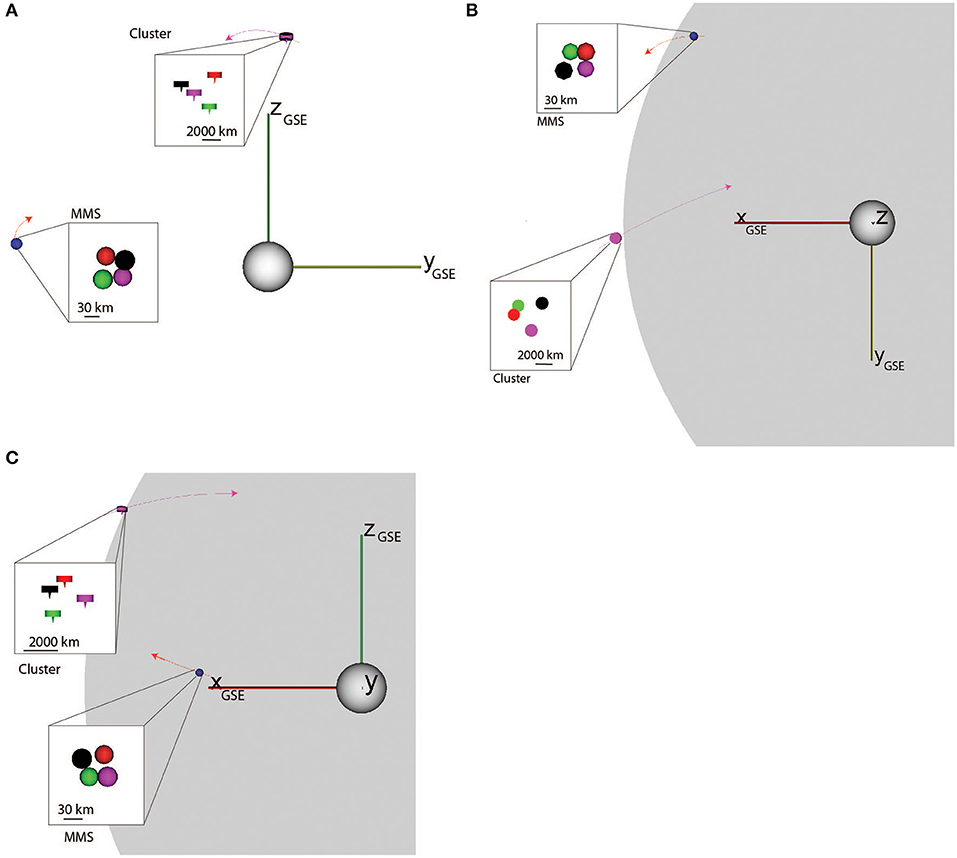
Figure 1. Cluster and MMS position on 7 February 2017 at 00:40 UT in YZGSE (A), XYGSE (B), and XZGSE (C). The spacecraft configuration and size of the tetrahedron is shown in the small insets. Cluster and MMS are shown in classical colors: number 1 in black, 2 in red, 3 in green, and 4 in magenta. The shape of the Cluster spacecraft is represented as a flat cylinder with an arrow along the spin axis. The MMS spacecraft are shown as spheres. The magnetopause is shown in gray and the Cluster and MMS orbits in thin purple and red line, respectively.

Solar Wind Data

The solar wind data were obtained from the ACE spacecraft and propagated to the bow shock and are available from the OMNI high resolution database (King and Papitashvili, 2005). Figure 2 shows the magnetic field (Figures 2A–D), the solar wind density (Figure 2E), the solar wind speed (Figure 2F), the solar wind dynamic pressure (Figure 2G), and the Alfvén Mach number (Figure 2H). The IMF (Figure 2A) was around 4 nT at the beginning and at the end of the 2h interval. In between 00:35 UT and 01:07 UT it decreased to values below 2 nT and as low as 0.38 nT at 01:00 UT. The IMF-Bz component (Figure 2B) was negative around −2 nT at the beginning of the interval up to 00:40 UT, then was around 0 nT up to 01:07 UT and again negative around −1.5 nT after that time. The IMF-By component was positive around 1 nT at the beginning of the interval, then around 0 nT between 00:35 UT and 01:07 UT and then negative after that time around −3 nT. The IMF-Bx component was negative around −2 nT at the beginning and at the end of the interval and positive in the middle, between 00:40 UT and 01:07 UT. Note that between 00:40 UT and 01:07 UT, the IMF was almost purely radial with a dominant IMF-Bx component. The cone angle (Figure 2D black line) showed large values in the range 100–130° up to 00:35 UT, then decreased to below 40° for a few minutes and then increased to above 150° for 5 min. After 00:41 UT, it decreased below 30° up to around 01:07 UT, except during a few minutes at 00:57 UT. After 01:07 UT, the cone angle was stable around 130° for 20 min and then slowly decreased down to 90°. The cone angle was therefore small (Bx dominant) between 00:33 UT and 01:07 UT. To check the propagation time of OMNI data we added THEMIS-B magnetic data on Figure 2C and the THEMIS-B cone angle in Figure 2D (red line). THEMIS B was in the solar wind close to the bow shock on the dusk side (XYZ_GSE = [−35, 48, −4.9] R_E) and downstream of the terminator. We have shifted the data by −9 min to take into account the propagation to the bow shock. THEMIS-B data agree well with OMNI data from 00:00 to 00:30 UT, then it observed the change to low cone angle around 00:32 UT which is about 8 min before OMNI data. THEMIS-B started to observe reflected ions and waves after 00:40 UT and we did not include data afterwards. This shows that OMNI data can have some inaccuracy in time and changes in solar wind can be out by a few minutes or a few 10s of minutes when reaching the bow shock as shown by Case and Wild (2012).

FIGURE 2

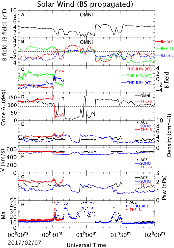
Figure 2. OMNI, THEMIS-B, and SOHO data propagated to the bowshock on 7 February 2017 between 00 and 02 UT. From top to bottom the panels show the OMNI total magnetic field (A), OMNI B-field components in GSM (B), THEMIS-B B-field components in GSM (C), the cone angle [ArcCos(Bx/B)] (D), the solar wind density (E), velocity (F), dynamic pressure (G), and the Alfvén Mach number (H).

Although showing three gaps of around 10 min, the plasma solar wind data showed rather constant values throughout the 2 h interval with a density around 3 cm⁻³ (Figure 2D), a speed around 540 km s⁻¹ (Figure 2E), producing a solar wind dynamic pressure around 1.6 nT (Figure 2F). The solar wind speed is therefore faster and the density lower than average solar wind values. SOHO data with a time shift of 37 min. and THEMIS-B are also shown on Figures 2E–H. There are some differences between these spacecraft, mainly in density, which may come from the different instruments or calibrations used on these spacecraft. Their different position in the solar wind could also explain these differences. Radial IMF, high solar wind speed and low solar wind density are usually associated with magnetosheath HSJs (Plaschke et al., 2013).

Cluster and MMS Observations

Figure 3 gives an overview of the event observed by Cluster 4 (C4), Cluster 1 (C1), and MMS1 ion and magnetic field data. The figure covers the same interval as in Figure 2, from 00:00 UT to 02:00 UT on 2017/02/07. The magnetosheath intervals are marked with a black bar at the bottom of the spectrograms on C4 and MMS1 (Figures 3a,g). Cluster was in the magnetosheath (high flux of ions from 100 eV to a few keVs) from the beginning of the interval up to around 01:07 UT when C4 crossed the magnetopause and entered the magnetosphere (substantial flux of high-energy ions above 10 keV). After about 10 min it went back into the magnetosheath for about 12 min and after 01:28 entered again in the magnetosphere for the rest of the interval. At 00:25 UT there was a change of mode of the ion instrument on C4 which explains the apparent change of flux in Figure 3a but the spacecraft stayed the whole time in the magnetosheath. The magnetic field measured by C4 and MMS1 (Figures 3c,i) was small and turbulent in the magnetosheath and large and slowly varying in the magnetosphere. C1 ion data (Figure 3d) are limited to a 1-h interval but the data are in the highest time resolution (4 s) between 00:08 UT and 01:10 UT. MMS1 was almost all the time in the magnetosheath except during a few intervals between 00:40 UT and 01:06 UT and around 01:35 UT.

FIGURE 3

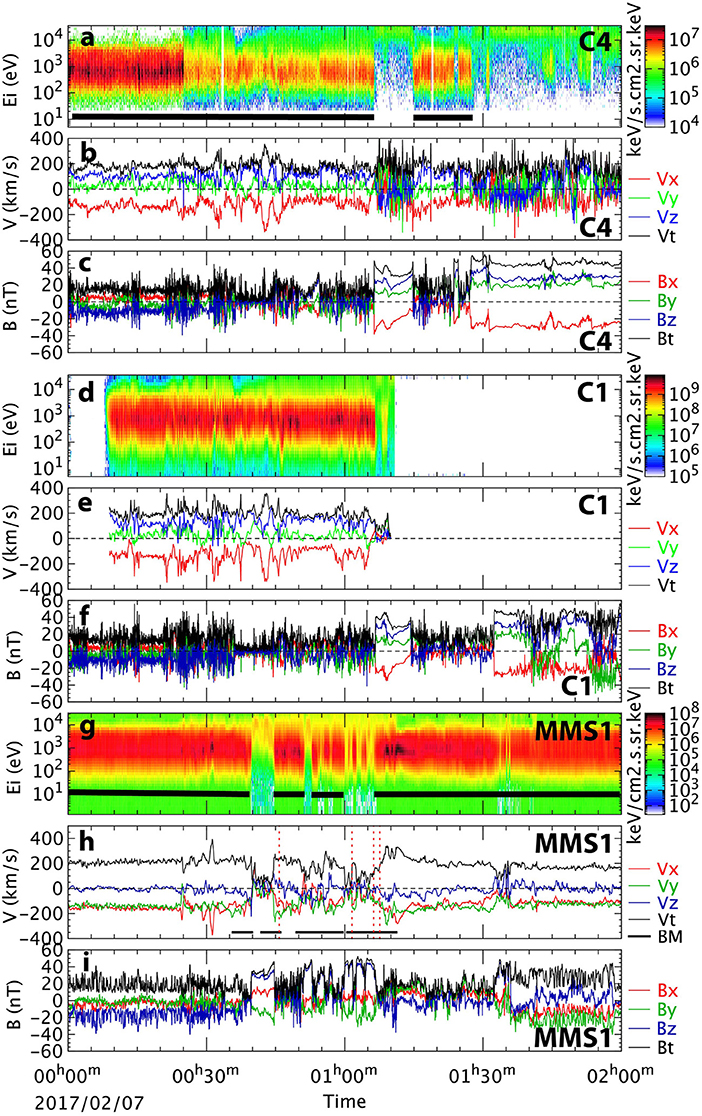
Figure 3. Cluster 4 (C4), Cluster 1 (C1) and MMS1 ion and magnetic field data on 7 February 2017 between 00 and 02 UT. Top three panels show the ion energy spectrogram (a), the velocity (b) and the magnetic field (c) from C4. Following panels are the same for C1 (d–f) and MMS1 (g–i). Magnetosheath intervals are indicated by thick black lines at the bottom of the spectrograms (a,g). MMS1 burst mode intervals are marked by thin black lines on the MMS1 velocity panel (h). Dust impact are marked as thin dotted red dashed lines on the MMS1 velocity panel (h).

The plasma speeds (Figures 3b,e,h) were larger with large plasma jets in the magnetosheath (V_x component dominant) and small in the magnetosphere. These jets are characterized by a strong V_x components (red line) lasting a few minutes and reaching a speed down to −350 km s⁻¹. On Cluster, they start from 00:04 UT on C4 up to the entry in the magnetosphere at 01:30 UT. On MMS the period where jets are visible starts later at around 00:25 UT. The other difference is that V_y is around 0 and V_z is positive on Cluster while V_y is negative and V_z is around 0 on MMS. This is most likely due to their different position with respect to the subsolar point, Cluster at mid-latitude in the northern hemisphere and MMS on the dawn flank. Table 1 lists the time and spacecraft observing the HSJs as well as their main properties such as the maximum speed, ion density, pressure, duration, and size.

TABLE 1

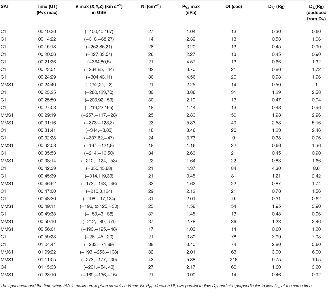
Table 1. High speed jets characteristics.

Magnetosheath HSJs

We will now focus on the HSJ observed around 00:31 UT which is seen around the same time on Cluster and MMS. Figure 4 shows C1 and MMS1 ion and magnetic field data between 00:25 UT and 00:35 UT on 2017/02/07. The Cluster ion (4 s temporal resolution) and magnetic field (5 vector/s) data are more variable than the ones measured by MMS1, although the temporal resolution is around the same for ions (around 4 s) and higher (16 vector/s) for the magnetic field on MMS1.

FIGURE 4

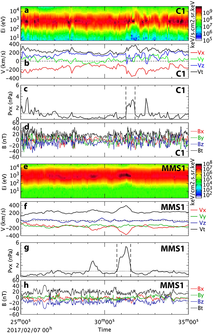
Figure 4. C1 and MMS1 ion and magnetic field data between 00:25 UT and 00:35 UT. Top four panels show the ion spectrograms (a), ion velocity (b), ion dynamic pressure using V_x component to identify HSJ (c) and magnetic field (d). Four bottom panel show the same parameters for MMS1 (e–h). Dotted horizontal line on the pressure plots (c,g) marks half of the solar wind dynamic pressure, around 0.99 nPa at 00:30:30 UT. Dashed vertical lines (c,g) identify the boundaries of the HSJs observed on C1 and MMS1.

We define the boundaries of the HSJs with the threshold when the ion dynamic pressure (${\text{nmV}}_{\text{x}}^2$) is half of the solar wind dynamic pressure (P_sw). Plaschke et al. (2013) defined the HSJs with 0.25 P_sw but in our case the factor 0.25 was found too low to isolate the HSJs, especially on MMS1. The boundaries of the HSJs are at 00:31:16 UT and 00:31:49 UT (dashed lines) in C1 data and 00:30:44 UT and 00:31:33 UT in MMS1 data. The HSJ is therefore starting 36 s earlier on MMS1 than on C1 and it is finishing 9 s earlier on MMS1. There is therefore an overlap in time of about of 24 s. The jet lasts longer in MMS1 (60 s) than in C1 (33 s) data and its peak in pressure is larger at MMS1 (5.3 nPa) than at C1 (3.5 nPa). These maxima of pressure are significantly larger than the pressure in the solar wind, which was around 2.0 nPa around that time.

Since there is a significant overlap in time, around 24 s, between the MMS1 and C1 HSJs, we could ask the question: is the HSJ seen on Cluster and MMS the same HSJ or are these two different HSJs? To address this question we estimate the size of these HSJs. We integrated the flow inside the HSJs using Equation (7) in Plaschke et al. (2016) and obtained D_//C1 = 1.2 R_E and D_//MMS1 = 2.6 R_E. The jet size observed by MMS1 is around 120% larger than the one observed by Cluster. If we assume a ratio between D_// and D_⊥ of ~0.5, based on Plaschke et al. (2016) jet multi-point statistical analysis, we obtain D_⊥C1 = 2.4 R_E and D_⊥MMS1 = 5.2 R_E. This assumption may not be valid for these HSJs since the HSJs studied in Plaschke et al. (2016) were smaller on average. The values estimated are, however, similar to the perpendicular size found by Gunell et al. (2014) based on a two-spacecraft analysis.

Figure 5 shows the position of Cluster and MMS and the HSJ detected at 00:31 UT, based on their estimated perpendicular size. Given the size of HSJs, the separation between Cluster and MMS seems too large to have detected the same jet and most likely each constellation detected a different jet. In addition, the jet direction is slightly different: it is pointing toward north on Cluster with V_xyz = (−344,−8,83) km s⁻¹ at 00:31:41 UT and toward dawn on MMS with V_xyz = (−373,−128,3) km s-1 at 00:31:16 UT.

FIGURE 5

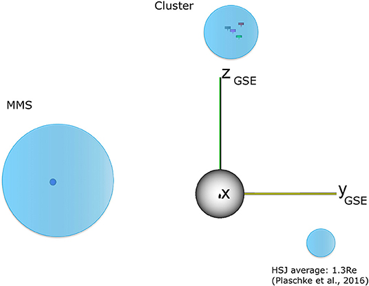
Figure 5. Position of MMS and Cluster in YZGSE plane at 00:31 UT. The HSJ observed by Cluster and MMS are shown as blue circles with the proper estimated size. For comparison the averaged size of HSJ from Plaschke et al. (2016) is show in the right bottom corner.

We will now analyze all HSJs observed during the 1.5 h interval by Cluster and MMS (see Table 1). During the first 24 min, only Cluster observed HSJs. MMS was in the magnetosheath at that time but only observed typical and fairly constant magnetosheath flows Vxyz (GSE) = (−150,−150,0) km s⁻¹ (see Figure 3). After 00:24:40 UT, HSJs are seen on both Cluster and MMS.

Figure 6 shows the maximum in V_x (Figure 6A), as well as V_y (Figure 6B), V_z (Figure 6C) and the magnitude V_t (Figure 6D) when V_x was maximum inside each HSJ. Cluster HSJs are shown in red asterisks and MMS ones in blue. Before 00:50 UT, the HSJs were faster, reaching values of V_x up to −380 km s⁻¹. After that time, the maximum reached was −280 km s⁻¹.

FIGURE 6

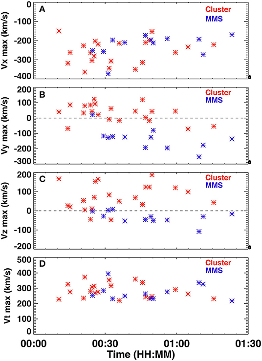
Figure 6. HSJs velocity components V_x (A), V_y (B), V_z (C), and total velocity V_t (D). HSJs observed by Cluster are marked with red asterisks and the ones observed by MMS are shown in blue asterisks.

V_y flows (Figure 6B) show a split between Cluster and MMS HSJs. The ones observed by Cluster have a positive V_y (median of 43 ± 57 km s⁻¹) and the ones seen by MMS exhibit negative V_y values (median of −125 ± 68 km s⁻¹). The variance between HSJs is quite large and there is some overlap between the one sigma interval on V_y measured by Cluster and MMS. Apart from the HSJ measured by MMS1 at 00:25 UT, the MMS and Cluster HSHs can be separated into two groups of different V_y. V_z is positive at Cluster (median of 68 ± 67 km s⁻¹) and in general negative at MMS (median of −30 ± 32 km s⁻¹) except between 00:20 and 00:35 UT. Finally, V_t does not show much difference between Cluster (median of 276 ± 47 km s⁻¹) and MMS (median of 263 ± 53 km s⁻¹), oscillating between 200 and 400 km s⁻¹. The HSJs have therefore a strong component in –Y direction at MMS location where its position in –Y was large (Figure 1A) and in +Z direction at Cluster location where its position in +Z was large. This may be due to their possible origin at the bow shock or to their propagation through the magnetosheath.

The dynamic pressure (P_Vx) values, calculated using the maximum V_x inside each HSJs, are plotted as a function of time in Figure 7A. Pvx varies from 1 up to 5.4 nPa throughout the intervals with no clear changes before and after 00:45 UT. Pvx seems larger on Cluster (median of 2.6 ± 1.1 nPa) than on MMS (median of 2.0 ± 1.5 nPa), however its variance is too large to draw any conclusion. When we compute the full dynamic pressure (nmV²) we found that the it is roughly the same at Cluster (3.7 ± 0.9 nPa) and at MMS (3.3 ± 1.9 nPa). Figure 7B shows that the duration of HJSs seems shorter Cluster (median of 21 ± 26 s) than at MMS (median of 36 ± 56 s), however, the variance is again too large to draw a conclusion.

FIGURE 7

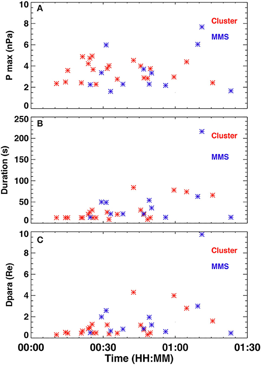
Figure 7. HSJs dynamic pressure Pvx (A), duration (B), parallel size Dpara (C). HSJs observed by Cluster are marked with a red star and the ones observed by MMS are shown in blue stars.

The size of the HSJs along the flow are given in Figure 7C. D_// shows an increase with time: starting low, below 2 R_E before 00:28 UT, and increasing up to almost 10 R_E at 01:11 UT. The estimate of the size of HSJs perpendicular to the flow (D_⊥) is done by assuming a ratio between D_// and D_⊥ of ~0.5, based on Plaschke et al. (2016) jet statistical analysis. HSJs seems larger at MMS (median D_//: 1.2 ± 2.6 R_E and D_⊥: 2.4 ± 5.2 R_E) than Cluster (median D_//: 0.7 ± 1.6 R_E and D_⊥: 1.4 ± 3.1 R_E). However, the variance is again too large to draw a definite conclusion. If we compute the median value of all HSJs seen by both Cluster and MMS, we obtain D_// = 0.8 ± 2.0 R_E and D_⊥ = 1.6 ± 4.0 R_E, which is similar to Plaschke et al. (2016) statistical size of D_// = 0.7 R_E and D_⊥ = 1.3 R_E. Most of HSJs D_⊥ (32 out of 33) are smaller than the separation between Cluster and MMS (around 10.6 R_E). Except one, however, that may be large enough to be observed by both constellations, assuming the factor 2 between D_// and D_⊥ also applies for large HSJs.

The two largest events are observed by Cluster at 00:42 UT and by MMS at 01:11 UT. Their size parallel to the flow is, respectively, 4.3 and 9.75 R_E. The distances of Cluster and MMS from the shock model of 2.2 and 3.6 R_E are smaller than these sizes. If we assume that HSJs are formed at the shock, this would mean that the HSJ duration is larger than the time it takes for them to cross the magnetosheath, in other words they would reach the magnetopause while still being connected to the bow shock. Another explanation could be that the large HSJs are formed by multiple HSJs merging together as they propagate through the magnetosheath. The large HSJ observed on MMS at 01:11:05 has a clear double peak in pressure (Figure 9G) at 01:10:15 UT and 01:11:05 UT and may be formed by two HSJs. We will look into more details at these two largest events and their impact on the magnetopause in the next section.

HSJs Impact on the Magnetopause

The first large HSJ was observed by Cluster at 00:42 UT. Given its estimated perpendicular size of 8.6 R_E, it could not have been observed by MMS which was around 10.6 R_E away from Cluster. MMS had entered the magnetosphere a few minutes earlier at 00:39:44 UT and entered again the magnetosheath at 00:44:45 UT. Figure 8 shows 10 min of C1 and MMS1 data (same format as Figure 4) around this HSJ. The maximum flow observed by C1 in V_x was −350 km s⁻¹ and the maximum of Pvx was 4.37 nPa. The two magnetopause crossings can be clearly seen on MMS1 data (Figures 8E–H) with the sharp change of energy in the ions going from sheath like plasma with energy around 1 keV to magnetospheric plasma with energy around 10 keV. A sharp change of magnetic field is also observed at the magnetopause with the B_z component varying from −17 nT up to +25 nT at 00:39: 44 UT and from +32 nT down to +5 nT at 00:44:45 UT (Figure 8H). The first magnetopause crossing shows a short negative V_z flow of −245 km s⁻¹ at 00:39:46 (Figure 8F, blue line), which was larger in absolute terms than the velocity components (V_x = −94 km s⁻¹ and V_y = −110 km s⁻¹). This may be an indication of reconnection taking place at the magnetopause between the southward magnetic field in the magnetosheath and the northward magnetic field in the magnetosphere. This aspect will however not be further studied in this paper.

FIGURE 8

Figure 8. C1 and MMS1 ion and magnetic field data between 00:37 UT and 00:47 UT (same format as Figure 4). Red lines on (C) and (G) show HSJs.

The MMS four-spacecraft analysis on the inbound magnetopause crossing at 00:39:44 UT gave a magnetopause normal equal to (0.30, 0.91,0.27)_GSE and a speed of −177 km s⁻¹ along the normal (see Table 2). Since the four spacecraft are very close to each other, such parameters are only valid within the very short time interval of the measurements and may not represent properly the magnetopause crossing. For comparison, we have used two other methods based on single spacecraft magnetic field and ion measurements: minimum variance analysis on B (MVAB) (Sonnerup and Scheible, 1998) and a combination of minimum Faraday residue analysis (MFR) and minimum variance analysis on V (MVAV) (Haaland et al., 2006; Sonnerup et al., 2006). For the crossing at 00:39:44 UT, the magnetopause normal with the timing analysis is mainly directed toward dusk (n_Y positive) while it is directed toward dawn (n_Y negative) with the MVAB and MFR+MVAV methods. Given the limitation of the timing method due to small spacecraft separations, we believe that the two other methods give, for this crossing, a better estimate of the normal and speed of the magnetopause. The magnetopause would be mainly directed toward dawn (as expected from the position of MMS in the dawn sector) and its speed would vary between 26 and 109 km s⁻¹.

TABLE 2

Table 2. Magnetopause crossing characteristics obtained with four-spacecraft analysis.

For the second outbound crossing at 00:44:45 UT, the direction of the normal obtained by the timing analysis was (0.93, 0.32, −0.20) with a speed of −139 km s⁻¹. For this crossing the other two methods (MVAB and MFR+MVAV) give similar orientation of the normal, mainly along X_GSE, with a speed ranging between 39 and 94 km s⁻¹. The inbound and outbound crossings show a very different normal with an angle of 62 and 84° between them, using MVAB and MFR+MVAV, respectively. The normal to the magnetopause model from Roelof and Sibeck (1993) at 00:39:44 UT was (0.79, −0.62, 0.05) _GSE and (0.79, −0.61, 0.06) at 00:44:45 UT (Table 2, 6th column). This is quite different from the MMS observations with an angle between MVAB and MFR+MVAV normals and the model in the range 31–52° at 00:39:44 UT and 36–44° at 00:44:45 UT. All magnetopause crossings observed during the HSJ period (6 by MMS and 2 by Cluster) are listed on Table 2. They all show a significant deviation from the Roelof and Sibeck (1993) magnetopause model, ranging from a minimum of 11° up to a maximum of 114°. Most likely HSJs indented the magnetopause and then the magnetopause rebounded, as observed previously by Shue et al. (2009). The indentation would explain the outbound crossings and the rebound would produce the inbound crossings. Since such deformation would be local, over around the size of the HSJ, the magnetopause on the sides of the indentation would have a normal making a significant angle with respect to the magnetopause model. Archer et al. (2019) showed THEMIS inbound and outbound magnetopause crossings with large deviation of their normal with respect to the model. They showed that an HSJ produced an indentation of the magnetopause and the subsequent formation of a standing surface wave.

The second largest HSJ was observed by MMS at 01:11:05 UT. Its estimated perpendicular size was 19.5 R_E. Similar to the previous one, Cluster entered the magnetosphere a few minutes before 01:11:05 UT and exit again in the magnetosheath a few minutes after. Figure 9 shows 10 min of data from Cluster 4 and MMS 1 (Cluster 4 was used since the ion instrument on C1 was switched off before the end of the interval). The HSJ observed by MMS (four bottom panels) is the longest observed during that day, 5 min long. Pvx goes slightly below the threshold of 0.5 Psw and therefore could be split into two HJSs of 1 and 3.5 min, respectively. This is supported by the change in the direction of the flow which is predominantly in –Y direction in the first one (–V_y dominant in 3rd panel from bottom) and –X in the second one (–V_x dominant).

FIGURE 9

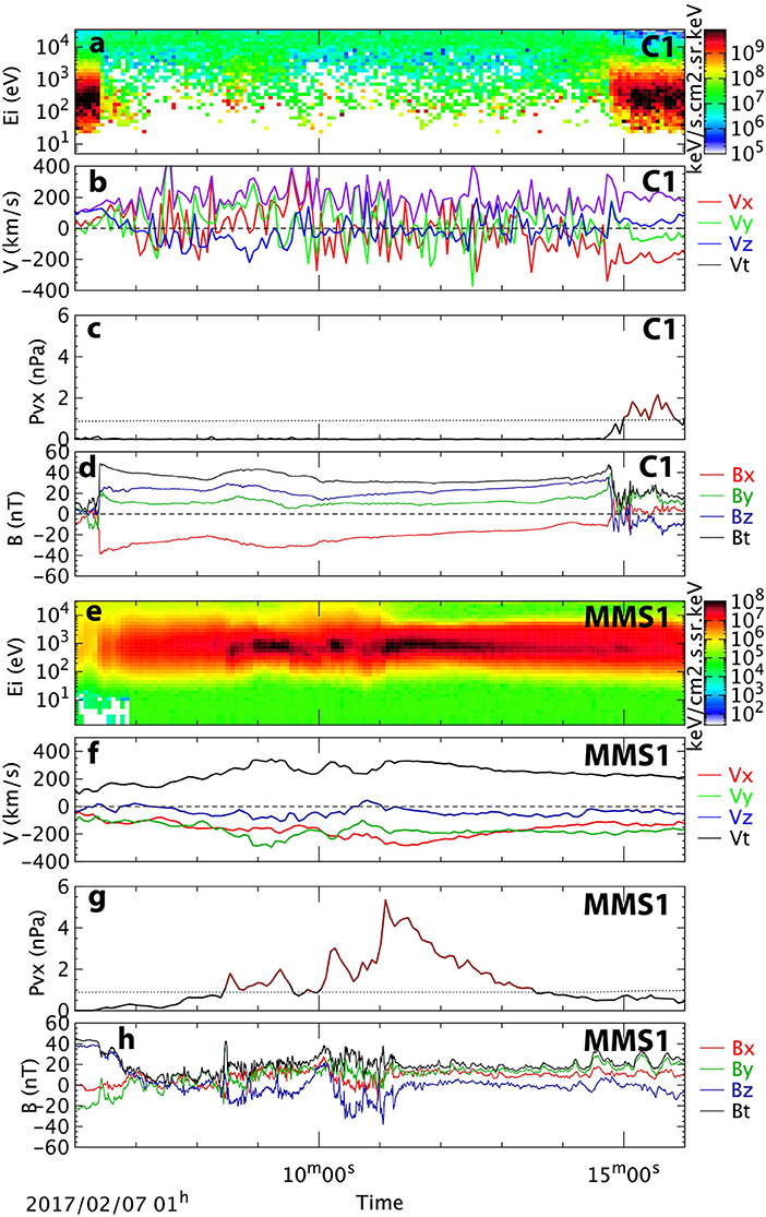
Figure 9. C1 and MMS1 ion and magnetic field data between 01:06 UT and 01:16 UT (same format as Figure 4). Red lines on (c) and (g) show HSJs.

Cluster went into the magnetosphere at 01:06:24 UT and exit in the magnetosheath at 01:14:47 (Figures 9A–D). Similar to MMS data, using the four spacecraft we computed the characteristics of the magnetopause. The normal direction given by the timing analysis during the first inbound crossing was (0.53, 0.23, 0.82)_GSE and the magnetopause speed around 142 km s⁻¹ along the normal. The second outbound crossing normal using the timing analysis was (0.85, −0.28, 0.44)_GSE and the magnetopause speed around −143 km s⁻¹. For Cluster the spacecraft being at larger separation (70 times) than MMS, the timing analysis is expected to be more accurate. Indeed, the two other methods, MVAB and MFR+MVAV give similar results. The Bz component of the magnetic field during these crossings is shown on Figures 10A,B. The inbound and outbound normals obtained from timing are different with about 42° between the two vectors. The normal to the magnetopause model at 01:06:24 UT was (0.84, 0.02, 0.53)_GSE and (0.84, 0.01, 0.54) _GSE at 01:14:47 UT. This is different from the Cluster observations with an angle between Cluster normals and the model of 28° at 01:06:24 UT and 17° at 01:14:47 UT. The MVAB and MFR+MVAV methods give an angle with the model normal between 11 and 32°. In these crossings the magnetopause was less deformed than in MMS crossings at 00:39:44 UT. Although this very large HSJ may have been extended over the Cluster-MMS constellation, there is no evidence that this was the case since the Cluster constellation was in the magnetosphere a few minutes around the HSJ.

FIGURE 10

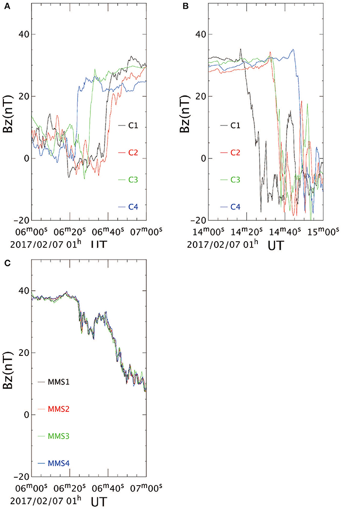
Figure 10. C4 and MMS1 magnetopause crossings on 7 February 2017. Magnetic field from Cluster at 01:06–01:07 UT (A) and at 01:14–01:15 UT (B) in GSE. Magnetic field from MMS at 01:06–01:07 UT (C) (same as A) in GSE.

An interesting aspect of the first inbound crossing of Cluster at 01:06:24 UT is that MMS also crossed the magnetopause at exactly the same time. The magnetopause crossing is shown in detail in Figure 10C with the same scale as the Cluster magnetopause crossing in Figure 10A. The Cluster and MMS magnetopause crossings are totally different (see Table 2 for detailed characteristics):

- Cluster crossing is inbound going from the magnetosheath to the magnetosphere and MMS is outbound going from the magnetosphere to the magnetosheath;

- Cluster crossings are sharp lasting on average 4 s while MMS crossings last 40 s;

- MMS crossing shows small structures within the magnetopause most likely due to back and forth motion of the magnetopause, while Cluster crossings are sharp;

- Since the MMS spacecraft separations are more than 70 times smaller than those between the Cluster spacecraft, the four MMS spacecraft are all in the magnetopause at the same time while Cluster crossings of the magnetopause are separated by about 6 s;

- The magnetopause normal at Cluster is mainly toward the Z and X direction, while MMS magnetopause normal is mainly along X (Table 2).

This shows that under the continuous impacts of HSJs, the magnetopause is deformed significantly and can even move in opposite directions at different places. It can therefore not be considered as a smooth surface anymore but more as surface full of local indents.

Nanodust Investigation

We investigate whether nanodust clouds were detected during some of these events. Solar wind data (Figure 2) do not show a cusp-like increase of magnetic field (Russell et al., 1983; Lai and Russell, 2018). At the beginning and at the end of the interval the IMF shows a total field around 4 nT and stable. In the middle of the event, the magnetic field decreases below 2 nT with some variability including some spikes at 00:37 UT and 01:26 UT. These were, however, below the 10 min minimum duration defined for IFEs by Lai and Russell (2018).

We then investigated if impacts of nanodust could be detected on the spacecraft. Dust impacts were detected in the past with electric field antenna as a short (a few ms) pulse of the spacecraft potential on Cluster (Vaverka et al., 2017) and MMS (Vaverka et al., 2018). Some large micro-meteorites/space debris were also detected on MMS with the accelerometers, attitude sensors, and electric field probes (Williams et al., 2016; Vaverka et al., 2018). In such case, the spacecraft potential pulse was lasting up to 1 s. We have looked for spacecraft potential pulses in the Cluster and MMS data during the 1 h 15 s when we see HSJs. To identify such pulses, we need wide band data on Cluster and burst mode data on MMS. Cluster recorded burst mode data, which was excluding wide band data acquisition, and therefore did not include probe potentials at a sufficiently high time resolution to investigate it. MMS, on the other hand, collected 3 intervals of about 10 min between 00:35 and 01:11, mainly centered on the magnetopause crossings (black bars on Figure 3h).

We analyzed the high-resolution spacecraft potential data (150 μs time resolution) and could identify four possible dust impacts. Two of these are shown on Figure 11. Left panel shows the event at 00:45:46.645 UT on MMS3 and right panel shows the second event was detected at 01:01:33.520 UT on MMS2. Both events are characterized by a sharp increase of the probe to spacecraft potential (top panels) of all 6 probes and then the slow decrease quickly after. The spacecraft potential (bottom panels) is calculated using the four spin probes (P1–P4), and corrected from the probe-plasma potential and other effects. Both events are characterized by a decrease of the spacecraft potential which is explained by a hypervelocity dust impact on the spacecraft body and subsequent recollection of impact cloud particles (e.g., Vaverka et al., 2018). The plasma around the spacecraft will then become denser and the spacecraft potential will decrease. Note that the scales of both events are very different with a change of spacecraft potential around 0.4 V at 00:45:46.645 UT and around 6 V at 01:01:33.520 UT. These events are very similar to Vaverka et al. (2018) dust impact identification on MMS data. A third and fourth events were detected at 01:06:16.580 UT on MMS3 with a spacecraft potential decrease of 1.5 V and at 01:07:36.906 UT on MMS2 with a spacecraft potential decrease of 0.15 V (not shown). The time of all four dust impacts are shown as dotted lines on Figure 3h.

FIGURE 11

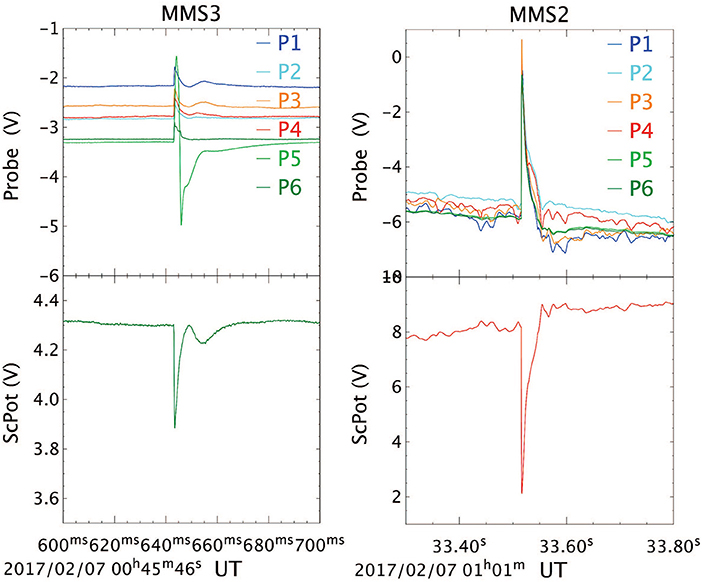
Figure 11. Dust impact observed on MMS3 (Left) and MMS2 (Right) at 00:45:46.645 UT and 01:01:33.520 UT, respectively. The top panels show the difference of potential between the 6 probes and the spacecraft (called probe potential). P1–P4 are the spin plane probes and P5 and P6 the spin axis probes. The bottom panels show the spacecraft potential calculated using the four spin probes (P1–P4), and corrected from the probe-plasma potential and other effects. Note that the scales are quite different in the two events.

Discussion and Conclusion

We have studied HSJs characteristics and their impact on the magnetopause at two widely separated points (10 R_E) across the dayside magnetosheath, using the Cluster and MMS constellations.

Our main observations can be summarized in the following:

- Many HSJs were observed at two very large separation over the dayside of the magnetosheath;

- IMF was radial with a low cone angle at the center of the event;

- HSJs were observed at Cluster 25 min before MMS;

- HSJs were characterized by a dominant V_x component with strong V_y at –Y position (MMS) and strong V_z components at –Z position (Cluster);

- 21 and 12 HJSs were observed by Cluster and MMS, respectively;

- Two HJSs were observed simultaneously at Cluster and MMS and given their characteristics and size, they would most likely be two separated HSJs;

- The largest HSJs observed, respectively, by Cluster and MMS had a computed size along the flow of 4.3 and 9.8 R_E and an estimated size of 8.6 and 19.6 R_E perpendicular to the flow;

- During these largest HSJs, when observed by one constellation, the other constellation had entered the magnetosphere a few minutes before and had left again a few minutes after;

- 6 and 2 magnetopause crossings were observed by MMS and Cluster during this interval with a significant angle, from 11° to 114°, between the normal given by the constellations and the normal given by the magnetopause model;

- One inbound magnetopause crossing observed by Cluster was observed simultaneous to an outbound magnetopause crossing of MMS;

- Four dust impacts were observed as a short pulse of the spacecraft potential between 00:45 UT and 01:10 UT on MM2 and MMS3 and no signature of dust cloud (IFE) was observed in the solar wind.

Cluster observed 7 HSJs before MMS observed its first one at 00:25 UT, 24 min later than the first one on Cluster. It has been shown previously that HSJs are predominantly observed behind a quasi-parallel shock (Hietala et al., 2009; Archer and Horbury, 2013; Plaschke et al., 2016), when the IMF makes an angle less than 45° with the shock normal. Figure 12A shows the Θ_Bn angle (between the IMF and the perpendicular to the bow shock surface) at 00:10 UT (before the IMF becomes radial) and at 00:48 UT (IMF radial). This shows that Cluster was behind the quasi-parallel shock (Θ_Bn < 45°) while MMS was behind a quasi-perpendicular shock (Θ_Bn larger than 45°) at 00:10 UT. This could explain why Cluster observe HSJs 24 min earlier than MMS. At 00:48 UT (Figure 12B), both Cluster and MMS are behind the quasi-parallel shock and both see HSJs around the same time. Under such IMF, the quasi-parallel shock would extend over the whole dayside of the magnetosphere, and it is expected to see HSJs on both Cluster and MMS although they are separated by 10 R_E. This shows that under such circumstances HSJs may cover a wide area of the front side magnetosphere as observed statistically by Plaschke et al. (2016).

FIGURE 12

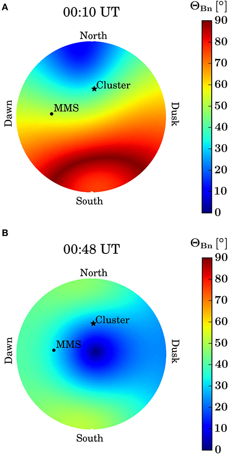
Figure 12. Θ_Bn angle (between the IMF and the bow shock normal) at 00:10 UT (A) and 00:48 UT (B) in GSE. The Cluster and MMS positions projected on the bow shock are show with a star and a dot, respectively. Θ_Bn of 45° (green) separate the quasi-parallel bow shock (blue) to the quasi-perpendicular bow shock (red/yellow).

The first MMS HSJ was observed at 00:24 UT. The first IMF cone angle (and therefore Θ_Bn) change was observed at 00:32 UT (THEMIS-B) 00:34 UT (OMNI). THEMIS-B timing may be more accurate than OMNI, since it was closer to the bow shock along X. THEMIS was, however, quite far away from the Sun-Earth line (Y_GSE = 48 R_E) and may also have some inaccuracy of a few minutes. We know that the IMF propagation from L1 to the bow shock can have inaccuracy of up to 20 min (Case and Wild, 2012), specially under radial IMF (Jelínek et al., 2010; Suvorova and Dmitriev, 2015). Such change in OMNI data may have therefore occurred 10–15 min before and could explain that MMS was behind a quasi-parallel bow shock and observing the first HSJ at 00:24 UT. The first turning of the Θ_Bn close to 0 may then have occurred a few minutes before the first MMS HSJ observation at 00:24 UT. MMS would then be connected to the parallel bow shock similar to 00:48 UT (Figure 12B).

The fact that a string of HSJs are observed at two points of the magnetosheath separated by 10 R_E shows that a large portion of the dayside magnetosphere may be impacted quasi-simultaneously by HSJs. Plaschke et al. (2016) assumed a circular surface of 5.7 R_E of radius centered around the Sun Earth line in his statistics. Our observations cover a wider area with Cluster at XYZ_GSE = [9.9, 0.3, 7.1] R_E and MMS at XYZ_GSE = [7.7, −8.0, 0.7] R_E. Enlarging the HSJs region, may increase the impact rates of 9 HSJs per hour obtained by Plaschke et al. (2016) for low cone angle. In our observations we detected 33 HSJs (adding Cluster and MMS) in 1 h 15 s and assuming that most of them are distinct, we get up to 26 per hour. This may also be underestimated if HSJs were also present in between Cluster and MMS and in other parts of the dayside magnetosphere. Plaschke et al. (2017) observed 18 HSJs with MMS in 58 min during low cone angle conditions, which is also higher than in his statistical analysis results. This shows that maybe other criteria such as high Mach number may need to be fulfilled, together with low IMF cone angle, for HSJs to be produced and in such cases, their frequency increases significantly when both criteria are met. Under the continuous impacts of HSJs, the magnetopause is deformed significantly and can even move in opposite directions at different places. It can therefore not be considered as a smooth surface anymore but more as surface full of local indents.

Figure 13A shows the HSJs observed by Cluster and MMS (black spots using median size of the observations) and Θ_Bn at 00:48 UT as background. Since we observed many HSJs at both Cluster and MMS, separated by 10 R_E, during 1.5 h, it is fair to assume that HSJs would be observed at other locations behind the quasi-parallel shock. Possible additional HSJs, with similar size as the ones observed at MMS and Cluster are sketched as spots in dashed line. The number of HSJs and the space in between is a pure assumption, but it illustrates that we may expect to see HSJs over the whole region of low Θ_Bn. Further investigation of other conjunctions between Cluster and MMS will be conducted to collect more events that may help to shed light on the spatial distribution of HSJ. New observations will also come in a few years when the THEMIS spacecraft will have their apogee aligned with Cluster and MMS. Figure 13B shows Cluster, MMS and THEMIS predicted simultaneous observations of the magnetosheath in 2020–2022. Double conjunctions will occur during many 100s of hours while triple conjunction with all three constellations at the same time in the magnetosheath would occur around 125 h.

FIGURE 13

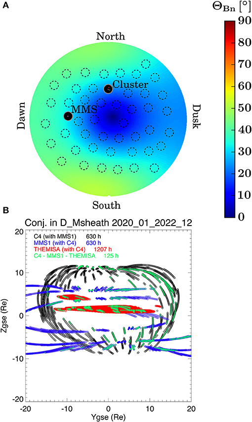
Figure 13. (A) Position and size of the HSJs (median Dperp) observed at Cluster and MMS. The background color is Θ_Bn at 00:48 UT. Circles with dashed lines show a sketch of similar HSJs that would be located behind the quasi-parallel bow shock; the space between and the size of these HSJs are purely hypothetical. (B) Future conjunctions of Cluster, MMS, and THEMIS in the magnetosheath in 2020–2022. The black symbols show the positions of Cluster 4 when it would be in the magnetosheath at the same time as MMS1. The blue symbols show the positions of MMS1 when it would be in the magnetosheath at the same time as Cluster 4. The red symbols show the positions of THEMIS-A when it would be in the magnetosheath at the same time as Cluster 4. Finally, the green symbols show the positions of all three spacecraft when they would at the same time in the magnetosheath. The number of hours indicated is the cumulated time of the conjunctions.

Could the magnetopause crossings by one constellation be related to the HSJ observed by the other? The inbound crossing observed by one constellation (00:39:44 UT with MMS and 01:06:24 UT with Cluster) would not be related to the HSJ observed by Cluster at 00:42 UT and by MMS at 01:11:05 UT since these are observed a few minutes after the magnetopause crossing and they would still need a few additional 10s of second to reach the magnetopause. The outbound crossing however at 00:44:45 UT with MMS and at 01:14:47 UT with Cluster could be related. Both of these crossings are fast −139 and −143 km s⁻¹ and show a deviation from the model magnetopause of 59° and 17°, respectively. The large size of these HSJs (D_⊥ = 8.6 and 19.5 R_E) would compress a large part of the dayside magnetosphere and the magnetopause may be pushed through a spacecraft even at 10 R_E away.

The main possible source of HSJs could be either solar wind discontinuities, solar wind dust cloud or bow shock ripples. Solar wind discontinuities would not explain all the HSJs observed, especially the ones between 00:10 UT and 00:30 UT which occur under stable solar wind IMF. Dust clouds signatures (IFE) were not observed in the solar wind, however, smaller clouds passing through the spacecraft in <10 min cannot be excluded. On the other hand, four signatures of dust impact were observed on MMS. These dust impacts could only be observed in burst data that was limited to three periods of 10 min. These burst intervals are around magnetopause crossing and not in the magnetosheath proper. None of these impacts are occurring simultaneously with the observation of HSJs, although we observed strong flows in the Y direction for three of them (see Figure 3). Four HSJs however have been observed in burst mode (00:38:14 UT, 00:50:10 UT, 00:56:01 UT, 01:09:22 UT, part of 01:11:05 UT) and did not show impact of dust on the spacecraft potential within 10s of seconds or few minutes of their duration. To draw a conclusion on the causality of dust on HSJs would require more events. However, the number of dust impact is still low and we would need more dust impacts and HSJs to exclude the dust clouds from the source of HSJs. Such investigation is however beyond of the scope of the current study. To our knowledge, however, this is the first time that dust impacts are indeed observed around the time of the HSJs observations. It is difficult to compare to statistics of nanodust impacts observed in the solar wind, on average 13 per day (Kellogg et al., 2016), with so few events but if we consider 2 events on MMS3 or MMS2 in 30 min, by extrapolation we would obtain 96/day. This is higher than the maximum rate of 62/day observed by Kellogg et al. (2016), however given the low number of events and the short interval of the MMS observation, it may not be significantly higher than the dust impacts observed in the solar wind.

The last process that would produce HSJs is bow shock ripples (Hietala et al., 2009) when the IMF is radial and the solar wind Mach number is above 10. Our event shows a radial IMF in the center of the event and the Alfvén Mach number was above 10 throughout the interval considered (Figure 2G), therefore it would fulfill Hietala et al. (2009) criteria for bow shock ripples and the subsequent penetration of HSJs in the magnetosheath. There is no spacecraft however in our event that could confirm the bow shock ripples. The fact that the HSJs have a -Y velocity component on the dawnside (MMS observations) and a +Z velocity component at mid latitude in the north hemisphere (Cluster observations) may indicate a link with the bow shock. It may also be a signature of the large scale magnetosheath flow diversion around the magnetopause. The fact that Cluster observed HSJs 25 min before MMS, which seems to be linked to the extent of the quasi-parallel bow shock (Figure 12), would also favor this process. Future conjunctions should however help to better constraint the HJSs source process by having spacecraft measuring at the same time the region upstream and downstream of the bow shock, the bow shock itself, magnetosheath HSJs and their impact on the magnetopause (Figure 13B).

Data Availability Statement

The Cluster, MMS, and THEMIS/OMNI datasets for this study can be found in the Cluster science Archive at http://csa.esac.esa.int, the MMS science data center at https://lasp.colorado.edu/mms/sdc/public/ and the NASA Space Physics Data Facility at https://omniweb.sci.gsfc.nasa.gov, respectively.

Author Contributions

CE did the data analysis and wrote the manuscript. K-JH and ST-R co-chair the ISSI working group where this study was conducted and provided comments. LT provided Figure 12 and part of Figure 13 and comments on the paper. SH provided support for the magnetopause normal computations and comments on the paper. NA, JD, JE, RF, HF, KG, DG, YK, GL, BL, CN, DS, and AV participated to the ISSI working group. JB, AD, GP, MD, YB, OR, HL, AM, MT, and PK provided comments to the manuscript. CC, ID, AF, RN, JB, BG, CP, CR, and RT provided the Cluster and MMS data through the Cluster archive and MMS data center.

Funding

The work of LT is supported by the Academy of Finland (Grant No. 322544). This research was supported by the NASA Magnetospheric Multiscale Mission in association with NASA contract NNG04EB99C. The work at UCLA was supported through subcontract 06-001 with the University of New Hampshire. RF was supported by STFC Consolidated Grant ST/R000719/1. MD was supported by NSFC grants 41874193 and 41821003. ST-R acknowledges support of the Ministry of Economy and Competitiviness (MINECO), Spain, Grant No. FIS2017-90102-R. PK's work was supported by PAPIIT grant IA101118. K-JH was, in part, supported by NSF AGS-1834451, NASA 80NSSC18K1534, 80NSSC18K0570, 80NSSC18K0693, and 80NSSC18K1337. ID thanks CNES for its support. JE acknowledges UKRI/STFC grant ST/N000692/1. YB was supported by the STFC RAL Space in House Research funding. Work of YK was supported by the Swedish National Space Board.

Conflict of Interest

The authors declare that the research was conducted in the absence of any commercial or financial relationships that could be construed as a potential conflict of interest.

The handling editor declared a past co-authorship with one of the authors GL.

Acknowledgments

We acknowledge the Cluster and MMS PIs, the Cluster Science archive (https://csa.esac.esa.int) and the MMS data center (https://lasp.colorado.edu/mms/sdc/public/) for making the Cluster and MMS best calibrated data available. The Space Physics data Facility at NASA/GSFC is also acknowledged for providing the OMNI data set and V. Angelopulous and the THEMIS team for providing the THEMIS B data. Data analysis was done with the QSAS science analysis system provided by the United Kingdom Cluster Science Center (Imperial College London and Queen Mary, University of London) supported by The Science and Technology Facilities Council (STFC), specially T. Allen and S. Schwartz, and SH for the magnetopause normal analysis plug-ins. The OVT team (https://ovt.irfu.se) is greatly acknowledged. We finally acknowledge the International Space Science Institute (ISSI) for supporting the team called MMS and Cluster observations of magnetic reconnection led by two authors of this paper (K-JH and ST-R).

References

Amata, E., Savin, S. P., Ambrosino, D., Bogdanova, Y. V., Marcucci, M. F., Romanov, S., et al. (2011). High kinetic energy density jets in the earth's magnetosheath: a case study. Planet. Space Sci. 59, 482–494. doi: 10.1016/j.pss.2010.07.021

CrossRef Full Text | Google Scholar

Archer, M. O., Hietala, H., Hartinger, M. D., Plaschke, F., and Angelopoulos, V. (2019). Direct observations of a surface eigenmode of the dayside magnetopause. Nat. Commun. 10:615. doi: 10.1038/s41467-018-08134-5

PubMed Abstract | CrossRef Full Text | Google Scholar

Archer, M. O., and Horbury, T. S. (2013). Magnetosheath dynamic pressure enhancements: occurrence and typical properties. Annal. Geophys. 31, 319–331. doi: 10.5194/angeo-31-319-2013

CrossRef Full Text | Google Scholar

Archer, M. O., Horbury, T. S., and Eastwood, J. P. (2012). Magnetosheath pressure pulses: generation downstream of the bow shock from solar wind discontinuities. J. Geophys. Res. 117:A05228. doi: 10.1029/2011JA017468

CrossRef Full Text | Google Scholar

Axford, W. I., and Hines, C. O. (1961). A unifying theory of high-latitude geophysical phenomena and geomagnetic storms. Can. J. Phys. 39, 1433–1464. doi: 10.1139/p61-172

CrossRef Full Text | Google Scholar

Baker, D. N., Riesberg, L., Pankratz, C. K., Panneton, R. S., Giles, B. L., Wilder, F. D., et al. (2016). Magnetospheric multiscale instrument suite operations and data system. Space Sci. Rev. 199, 545–575. doi: 10.1007/s11214-014-0128-5

CrossRef Full Text | Google Scholar

Balogh, A., Carr, C. M., Acuña, M. H., Dunlop, M. W., Beek, T. J., Brown, P., et al. (2001). The cluster magnetic field investigation: overview of in- flight performance and initial results. Ann. Geophys. 19:1207. doi: 10.5194/angeo-19-1207-2001

CrossRef Full Text | Google Scholar

Burch, J. L., Moore, T. E., Torbert, R. B., and Giles, B. L. (2016). Magnetospheric multiscale overview and science objectives. Space Sci. Rev. 199, 5–21. doi: 10.1007/s11214-015-0164-9

CrossRef Full Text | Google Scholar

Cahill, L. J., and Amazeen, P. G. (1963). The boundary of the geomagnetic field. J. Geo. phys. Res. 68, 1835–1843. doi: 10.1029/JZ068i007p01835

CrossRef Full Text | Google Scholar

Case, N. A., and Wild, J. A. (2012). A statistical comparison of solar wind propagation delays derived from multispacecraft techniques. J. Geophys. Res. 117:A02101. doi: 10.1029/2011JA016946

CrossRef Full Text | Google Scholar

Dungey, J. W. (1961). Interplanetary magnetic field and the auroral zone. Phys. Res. Lett. 6:47. doi: 10.1103/PhysRevLett.6.47

CrossRef Full Text | Google Scholar

Ergun, R. E., Tucker, S., Westfall, J., Goodrich, K. A., Malaspina, D. M., Summers, D., et al. (2016). The axial double probe and fields signal processing for the MMS mission. Space Sci. Rev. 199, 167–188. doi: 10.1007/s11214-014-0115-x

CrossRef Full Text | Google Scholar

Escoubet, C. P., Fehringer, M., and Goldstein, M. (2001). The cluster mission. Ann. Geophys. 19, 1197–1200. doi: 10.5194/angeo-19-1197-2001

CrossRef Full Text | Google Scholar

Gunell, H., Stenberg Wieser, G., Mella, M., Maggiolo, R., Nilsson, H., and Darrouzet, F. (2014). Waves in high-speed plasmoids in the magnetosheath and at the magnetopause. Ann. Geophys. 32, 991–1009. doi: 10.5194/angeo-32-991-2014

CrossRef Full Text | Google Scholar

Haaland, S., Sonnerup, B. U. O., Paschmann, G., Georgescu, E., Dunlop, M. W., Balogh, A., et al. (2006). Discontinuity Analysis with Cluster, in Cluster and Double Star Symposium, ESA SP-598. Noordwijk: ESA Publications Division.

Heikkila, W. J. (1982). Impulsive plasma transport through the magnetopause. Geophys. Res. Lett. 9, 159–162. doi: 10.1029/GL009i002p00159

CrossRef Full Text | Google Scholar

Hietala, H., Laitinen, T. V., Andréeová, K., Vainio, R., Vaivads, A., and Palmroth, M. (2009). Supermagnetosonic jets behind a collisionless quasiparallel shock. Phys. Rev. Lett. 103:245001. doi: 10.1103/PhysRevLett.103.245001

PubMed Abstract | CrossRef Full Text | Google Scholar

Hietala, H., and Plaschke, F. (2013). On the generation of magnetosheath high-speed jets by bow shock ripples. J. Geophys. Res. 118, 7237–7245. doi: 10.1002/2013JA019172

PubMed Abstract | CrossRef Full Text | Google Scholar

Jelínek, K., Němeček, Z., Šafránková, J., Shue, J.-H., Suvorova, A. V., and Sibeck, D. G. (2010). Thin magnetosheathas a consequence of the magnetopause deformation: THEMIS observations. J. Geophys. Res. 115:A10203. doi: 10.1029/2010JA015345

CrossRef Full Text | Google Scholar

Johnstone, A. D., Alsop, C., Burge, S., Carter, P. J., Coates, A. J., Coker, A. J., et al. (1997). PEACE: a plasma electron and current experiment. Space Sci. Rev. 79, 351–398. doi: 10.1007/978-94-011-5666-0_13

CrossRef Full Text | Google Scholar

Karlsson, T., Brenning, N., Nilsson, H., Trotignon, J.-G., Valliéres, X., and Facsko, G. (2012). Localized density enhancements in the magnetosheath: three-dimensional morphology and possible importance for impulsive penetration. J. Geophys. Res. 117:A03227. doi: 10.1029/2011JA017059

CrossRef Full Text | Google Scholar

Kellogg, P. J., Goetz, K., and Monson, S. J. (2016). Dust impact signals on the wind spacecraft. J. Geophys. Res. Space Phys. 121, 966–991. doi: 10.1002/2015JA021124

CrossRef Full Text | Google Scholar

King, J. H., and Papitashvili, N. E. (2005). Solar wind spatial scales in and comparisons of hourly wind and ACE plasma and magnetic field data. J. Geophys. Res. 110:A02104. doi: 10.1029/2004JA010649

CrossRef Full Text | Google Scholar

Laakso, H., Taylor, M., and Escoubet, C. P., (eds.) (2010). “The cluster active archive,” in Astrophysics and Space Science Proceedings (New York, NY: Springer).

Google Scholar

Lai, H. R., and Russell, C. T. (2018). Nanodust released in interplanetary collisions. Planet. Space Sci. 156, 2–6. doi: 10.1016/j.pss.2017.10.003

CrossRef Full Text | Google Scholar

Lemaire, J., and Roth, M. (1978). Penetration of solar wind plasma elements into the magnetosphere. J. Atmos. Terr. Phys. 40, 331–335 doi: 10.1016/0021-9169(78)90049-1

CrossRef Full Text | Google Scholar

Lindqvist, P., Olsson, G., Torbert, R. B., King, B., Granoff, M., Rau, D., et al. (2016). The spin-plane double probe electric field instrument for MMS. Space Sci. Rev. 199, 137–165. doi: 10.1007/s11214-014-0116-9

CrossRef Full Text | Google Scholar

Liu, Y. Y., Fu, H. S., Liu, C. M., Wang, Z., Escoubet, P., Hwang, K.-J., et al. (2019). Parallel electron heating by tangential discontinuity in turbulent magnetosheath. Astrophys. J. Lett. 877:L16. doi: 10.3847/2041-8213/ab1fe6

CrossRef Full Text | Google Scholar

Malaspina, D., and Wilson, L. B. (2016). A database of interplanetary and interstellar dust detected by the wind spacecraft. J. Geophys. Res. Space Phys. 121, 9369–9377. doi: 10.1002/2016JA023209

CrossRef Full Text | Google Scholar

Meyer-Vernet, N., Maksimovic, M., Czechowski, A., Mann, I., Zouganelis, I., Goetz, K., et al. (2009). Dust detection by the wave instrument on STEREO: nanoparticles picked up by the solar wind? Sol. Phys. 256, 463–474. doi: 10.1007/s11207-009-9349-2

CrossRef Full Text | Google Scholar

Miura, A. (1984). Anomalous transport by magnetohydrodynamic kelvin-helmholtz instabilities in the solar wind-magnetosphere interaction. J. Geophys. Res. 89, 801–818. doi: 10.1029/JA089iA02p00801

CrossRef Full Text | Google Scholar

Moore, T. W., Nykyri, K., and Dimmock, A. P. (2016). Cross-scale energy transport in space plasmas. Nat. Phys. 12, 1164–1169. doi: 10.1038/nphys3869

CrossRef Full Text | Google Scholar

Nemecěk, Z., Šafránková, J. M., Prech, L., Sibeck, D. G., Kokubun, S., Mukai, T., et al. (1998). Transient flux enhancements in the magnetosheath. Geophys. Res. Lett. 25, 1273–1276. doi: 10.1029/98GL50873

CrossRef Full Text | Google Scholar

Plaschke, F., Hietala, H., and Angelopoulos, V. (2013). Anti-sunward high-speed jets in the subsolar magnetosheath. Annal. Geophys. 31, 1877–1889. doi: 10.5194/angeo-31-1877-2013

CrossRef Full Text | Google Scholar

Plaschke, F., Hietala, H., Angelopoulos, V., and Nakamura, R. (2016). Geoeffective jets impacting the magnetopause are very common. J. Geophys. Res. Space Phys. 121, 3240–3253. doi: 10.1002/2016JA022534

PubMed Abstract | CrossRef Full Text | Google Scholar

Plaschke, F., Hietala, H., Archer, M., Blanco-Cano, X., Kajdič, P., Karlsson, T., et al. (2018). Jets downstream of collisionless shocks. Space Sci. Rev. 214:81. doi: 10.1007/s11214-018-0516-3

CrossRef Full Text | Google Scholar

Plaschke, F., Karlsson, T., Hietala, H., Archer, M., Vörös, Z., Nakamura, R., et al. (2017). Magnetosheath high-speed jets: internal structure and interaction with ambient plasma. J. Geophy. Res. 122, 10157–10175. doi: 10.1002/2017JA024471

CrossRef Full Text | Google Scholar

Pollock, C., Moore, T., Jacques, A., Burch, J., Gliese, U., Saito, Y., et al. (2016). Fast plasma investigation for magnetospheric multiscale. Space Sci. Rev. 199, 331–406. doi: 10.1007/s11214-016-0245-4

CrossRef Full Text | Google Scholar

Rème, H., Aoustin, C., Bosqued, J. M., Dandouras, I., Lavraud, B., Sauvaud, J. A., et al. (2001). First multispacecraft ion measurements in and near the earth's magnetosphere with the identical cluster ion spectrometry (CIS) experiment. Ann. Geophys. 19, 1303–1354. doi: 10.5194/angeo-19-1303-2001

CrossRef Full Text | Google Scholar

Roelof, E.-C., and Sibeck, D. G. (1993). Magnetopause shape as a bivariate function of interplanetary magnetic field Bz and solar wind dynamic pressure. J. Geophys. Res. 98, 21421–21450. doi: 10.1029/93JA02362

CrossRef Full Text | Google Scholar

Russell, C. T., Anderson, B. J., Baumjohann, W., Bromund, K. R., Dearborn, D., Fischer, D., et al. (2016). The magnetospheric multiscale magnetometers. Space Sci. Rev. 199, 189–256. doi: 10.1007/s11214-014-0057-3

CrossRef Full Text | Google Scholar

Russell, C. T., Luhmann, J. G., Barnes, A., Mihalov, J. D., and Elphic, R. C. (1983). An unusual interplanetary event: encounter with a comet? Nature 305, 612–615. doi: 10.1038/305612a0

CrossRef Full Text | Google Scholar

Savin, S., Amata, E., Zelenyi, L., Budaev, V., Consolini, G., Treumann, R., et al. (2008). High kinetic energy jets in the earth's magnetosheath: implications for plasma dynamics and anomalous transport. JETP Lett. 87, 593–599. doi: 10.1134/S0021364008110015

CrossRef Full Text | Google Scholar

Savin, S. P., Zelenyi, L. M., Amata, E., Buechner, J., Blecki, J., Klimov, S. I., et al. (2004). Dynamic interaction of plasma flow with the hot boundary layer of a geomagnetic trap. JETP Lett. 79, 368–371. doi: 10.1134/1.1772433

CrossRef Full Text | Google Scholar

Shue, J.-H., Chao, J.-K., Song, P., McFadden, J. P., Suvorova, A., Angelopoulos, V., et al. (2009). Anomalous magnetosheath flows and distorted subsolar magnetopause for radial interplanetary magnetic fields. Geophys. Res. Lett. 36:L18112. doi: 10.1029/2009GL039842

CrossRef Full Text | Google Scholar

Sonnerup, B. U. O., Haaland, S., Paschmann, G., Dunlop, M. W., Réme, H., and Balogh, A. (2006). Orientation and motion of a plasma discontinuity from single-spacecraft measurements: generic residue analysis of cluster data. J. Geophys. Res. 111:A05203. doi: 10.1029/2005JA011538

CrossRef Full Text | Google Scholar

Sonnerup, B. U. O., and Scheible, M. (1998). “Minimumand maximum variance analysis,” in Analysis Methods for Multi-Spacecraft Data, eds G. Paschmann and P. W. Daly (Noordwijk: ESA Publications Division), 185–220.

Google Scholar

Suvorova, A. V., and Dmitriev, A. V. (2015). Magnetopause inflation under radial IMF: comparison of models. Earth Space Sci. 2, 107–114. doi: 10.1002/2014EA000084

CrossRef Full Text | Google Scholar

Torbert, R. B., Russell, C. T., Magnes, W., Ergun, R. E., Lindqvist, P.-A., LeContel, O., et al. (2016). The FIELDS instrument suite on MMS: scientific objectives, measurements, and data products. Space Sci. Rev. 199, 105–135. doi: 10.1007/s11214-014-0109-8

CrossRef Full Text | Google Scholar

Vaverka, J., Nakamura, T., Kero, J., Mann, I. B., De Spiegeleer, A., Hamrin, M., et al. (2018). Comparison of dust impact and solitary wave signatures detected by multiple electric field antennas onboard the MMS spacecraft. Space Phys. Space Phys. 123, 6119–6129. doi: 10.1029/2018JA025380

CrossRef Full Text | Google Scholar

Vaverka, J., Pellinen-Wannberg, A., Kero, J., Mann, I., De Spiegeleer, A., Hamrin, M., et al. (2017). Detection of meteoroid hypervelocity impacts on the cluster spacecraft: first results. J. Geophys. Res. Space Phys. 122, 6485–6494. doi: 10.1002/2016JA023755

CrossRef Full Text | Google Scholar

Williams, T., Sulman, S., Sedlak, J., Ottenstein, N., and Lounsbury, B. (2016). Magnetospheric Multiscale Mission Attitude Dynamics: Observations from Flight Data. doi: 10.2514/6.2016-5675.

CrossRef Full Text | Google Scholar

Wing, S., Johnson, J. R., Chaston, C. C., Echim, M., Escoubet, C. P., Lavraud, B., et al. (2014). Review of solar wind entry into and transport within the plasma sheet. Space Sci. Rev. 184, 33–86. doi: 10.1007/s11214-014-0108-9

CrossRef Full Text | Google Scholar