Automatic Classification of Plasma Regions in Near-Earth Space With Supervised Machine Learning: Application to Magnetospheric Multi Scale 2016–2019 Observations

1. Introduction

Near-Earth space regions classification is a very challenging topic in space physics because of the strong plasma dynamics resulting from the interaction between the propagating solar wind and the standing Earth's magnetosphere. This obstacle forms a collisionless bow shock (Kivelson et al., 1995) which can reflect and backpropagate energetic ions into the supersonic solar wind, forming the ion foreshock region upstream. However, most of the plasma is decelerated and heated downstream to a subsonic flow which forms a sheath around the Earth's magnetosphere called the magnetosheath. The boundary on which magnetosheath and magnetospheric pressures balance is called the magnetopause. The plasma flows along the magnetopause toward the magnetotail, driving the frozen-in magnetic field lines through the lobes, plasma sheet boundary layer and ultimately the plasma sheet, in which they eventually reconnect (Dungey, 1963). This large-scale solar-terrestrial interaction process is dominated by the highly-variable solar wind conditions, but also by localized and intermittent small-scale processes in each region. As a result, the plasma throughout the near-Earth space is highly dynamic which make it impossible to classify the different regions using only spacecraft location along its orbit.

Yet, this classification is needed for statistical studies of the plasma properties of the different regions. These large-scale statistics are allowed by the ever-growing quantity of available in-situ data from space missions that cover most of the near-Earth space. A large amount of available data has been used to identify near-Earth space regions using human-driven (i.e., threshold-based) methods (e.g., Jelínek et al., 2012). However, finding the optimal set of thresholds which characterizes every region of the magnetosphere is time-consuming and presumably not flexible enough with regard to the large variability expected from the strong plasma dynamics. This may introduce important biases depending on the chosen thresholds, and may also result in many “unclassified” regions (i.e., a significant loss of information).

One way to bypass this issue and benefit from this large amount of data is to make use of supervised learning, the most common form of machine learning. The role of the supervised algorithms is to learn the relationship between data instances and an associated label for each data instance. For example, the text from an email may represent the data instance and the label is a binary encoding the presence or not of spam in order to detect and filter spams from emails. Supervised methods aim at expanding human knowledge automatically by identifying the intrinsic differences between labeled points in a dataset. This knowledge is then generalized to other unlabeled datasets. Such machine learning techniques show extremely promising (often state-of-the-art) results in various tasks, such as image and speech recognition, analyzing particle accelerator data, or natural language understanding (LeCun et al., 2015). They have already been used specifically in heliophysics: to classify time series into several categories defined by the solar origin of the wind (Camporeale et al., 2017), to detect magnetospheric ultra-low frequency waves (Balasis et al., 2019), to forecast solar flares (Nishizuka et al., 2017), or in particular to identify different regions of the near-Earth space (Nguyen et al., 2019; Olshevsky et al., 2019). Nevertheless, these models remain usually region- or mission-specific because the process of human-labeling is a time-consuming and tedious task and there is still a blatant lack of human labels to cover the whole near-Earth space.

However, the Magnetospheric Multi Scale mission (MMS) (Burch et al., 2016), launched in 2015 and whose orbit covers most of near-Earth space, has enabled such a dataset to be built. This mission uses the so-called Scientist In The Loop (SITL) system (see the following section for more details) to human-label phenomena and regions of interest. The SITL process involves that an expert scientist is designated to select data of interest that will be transmitted to the ground as high-time resolution (burst) data. The selected intervals are tagged with timestamps and a comment, which are reported in the SITL reports. This system has been active since July 2015 and thus provides more than 4 years of commented data as of now. This makes it the biggest dataset of commented events and regions to our knowledge. We developed an automatic parser to convert all the comments, written by different scientists, in a unified list of labels that can be used by a machine learning algorithm.

All SITL comments are associated with a time interval, therefore the temporal variations of the measurements can be used to predict the label of the signals. Thus, each data instance can be interpreted as a time series and the near-Earth classification using SITL data can be seen as a time series classification (TSC), a very challenging problem in data mining and machine learning (Esling and Agon, 2012; Fawaz et al., 2019). The main difference with classical classification problems comes from the ordering of the data. The important features helping to discriminate the labels are mainly found in the ordering of the values while classical methods only consider the values at a given time. We employ two different techniques to solve this multivariate and multicategory classification task: the multilayer perceptron is applied naively on instantaneous data and is considered as a baseline for comparison and the convolutional neural network is applied on time series.

In this article, we use the magnetic field and particle measurements of the MMS mission to establish a vast and reproducible automatic detection of 8 plasma regions that cover almost the entire near-Earth space. First, we introduce the MMS and Cluster missions, and how we used the SITL reports to build a large labeled dataset of magnetic field, plasma moments and plasma distributions from the 2016-2019 period. Then, we present the two machine learning algorithms we used and their characteristics, as well as the metrics to measure their performances. Later, we present their respective results for the MMS mission and the adaptation to the Cluster mission. Finally, we discuss these results and show our conclusions.

2. Data

A fundamental and time-consuming step in any machine learning application is collecting, cleaning, and labeling data. This is a very important task as the quality of the data defines accuracy and the generalization capability of the model.

2.1. The MMS and Cluster Missions

MMS is a NASA space mission, launched in 2015, designed to study the electron-scale physics in Earth's magnetosphere and in particular where magnetic reconnection occurs (Burch et al., 2016). Its equatorial orbit is optimized to spend extended periods in locations where reconnection is known to occur and thus covers the majority of the near-Earth space key regions. The mission is composed of four identical spacecraft flying in an adjustable tetrahedral formation and its highly-elliptic orbit also covers almost all regions of near-Earth space. The direct-current (DC) magnetic field data are provided by the Fluxgate Magnetometer (FGM) from the FIELDS instrument suite (Russell et al., 2016; Torbert et al., 2016) with a temporal resolution of 0.1s in “survey” mode and the plasma parameters by the Fast Plasma Investigation (FPI) instrument Pollock et al. (2016) with a temporal resolution of 4.5 s in “fast” mode.

Cluster is an ESA space mission, launched in 2000, whose aim is to study the ion-scale physics of Earth's magnetic environment and its interaction with the solar wind. The mission is also composed of four identical spacecraft flying in a tetrahedral formation and its highly-elliptic polar orbit also covers almost all regions of near-Earth space. The magnetic field data are provided by the Fluxgate Magnetometer with a temporal resolution of 4 s (Balogh et al., 2001) and the plasma parameters by the Hot Ion Analyzer instrument (Rème et al., 2001) when the instrument was working under the magnetosphere or the magnetosheath mode.

2.2. The Labels Datasets

One of the most important innovation brought by the MMS mission is its burst data management and selection system. The MMS spacecraft collect a combined volume of ~100 gigabits per day of particle and field data. On average, only 4 gigabits of that volume can be transmitted to the ground. With nested automation and “Scientist-in-the-Loop” (SITL) processes, this system is designed to maximize the value of the burst data by prioritizing the data segments selected for transmission to the ground.

Concretely, the SITL system consists of a manual selection process by a scientific expert designated to eyeball daily survey (low-time resolution) data and pick time intervals of interest that will be transmitted to the ground as burst (high-time resolution) data. The selected intervals are tagged with timestamps and a comment, which usually includes the type of event selected and eventually the near-Earth region in which it occurred. For each orbit, these selections are written up in a “SITL report,” in the form of a text file notably. An example of these reports can be found in Argall et al. (2020).

We developed a Python code which parses these text files to extract the timestamps and comments by identifying keywords associated with the near-Earth region where the event occurred. Each time interval was then associated with a label indicating where the spacecraft was located as follows.

If a region cannot be identified from the SITL comment, then the time interval is rejected. If FGM or FPI data is not available during a labeled time interval, then the time interval is also rejected. Using this technique, from the date at which the SITL reports are available as text files, i.e., April 2016, to the end of 2019, we collected 7, 832 labeled time intervals relevant for our study. We note here that the number of occurrences for each regions were somewhat unbalanced, so we added a total of 605 time intervals labeled by hand to undersampled regions (examples of typical plasma parameters for the different magnetospheric regions can be found in textbooks, e.g., Baumjohann and Treumann, 1996), bringing the total to 8, 437 labeled time intervals of various lengths. We resampled the label data to the same cadence as FPI data, i.e., 4.5 s, representing a total of 1, 331, 133 labeled data points. This constitutes the biggest dataset of labeled time intervals for near-Earth space to our knowledge. The labels of the different regions are sorted roughly according to their distance to the Sun, and summarized in Table 1.

TABLE 1

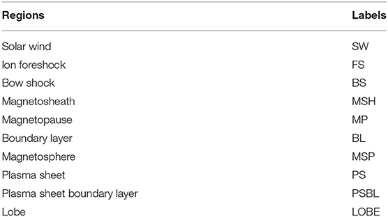
Table 1. Labels for the 10 different near-Earth regions in our model.

Regarding the Cluster mission labels, we use the dataset presented in Nguyen et al. (2019). This dataset covers three near-Earth space regions, namely the magnetosphere, the magnetosheath and the solar wind, over a 2-year time period (2005–2006). The data is resampled to a 1 min resolution, yielding a total of 148, 762 labeled points.

2.3. Final Data Set

Once the labels are defined, we build the final dataset that will feed the ML models. In Earth's magnetosphere, the plasma is dominated by its core magnetic field, thus the first feature we took into account is the magnetic field vector $\overrightarrow{B}$. Additionally, in each magnetospheric region the plasma has a rather typical distribution function. However, the full particle distribution function constitutes an enormous amount of data when dealing with several years of data (as done here), in particular with the MMS mission (several TB of data). Furthermore, important differences exist between different heliospheric missions in the specificities of the distribution functions, e.g., energy and angular ranges as well as energy and angular resolutions. Therefore, we chose not to consider those products and focused on moments only (density, bulk velocity and temperature), to keep our model lightweight and as general as possible (i.e., applicable to different heliospheric missions such as Cluster). For this latter reason, we also decided not to use the spacecraft location as a feature, because different missions cover different locations in near-Earth space (e.g., Cluster has a polar orbit while MMS has an equatorial orbit; apogees/perigees are different, etc.).

We start with loading the raw MMS magnetic field and plasma moments data from FGM and FPI instruments for the 2016–2019 period using the aidapy package¹, and resample the data to the FPI cadence, i.e., 4.5 s. The resulting dataset contains 12 variables: the magnetic field magnitude B_tot and its components B_x, B_y, B_z, the ion density N_i, the bulk velocity magnitude V_itot and its components V_ix, V_iy, V_iz, the parallel and perpendicular temperatures T_∥, T_⊥ with regards to the ambient magnetic field and the total value T_tot. The dataset is matched with the labels points defined in the previous section. If data gaps are present in the specified time interval, then the whole interval is rejected. This method yields a total dataset of size 1, 331, 133 × 12.

The TSC model requires as input arrays of equal sizes with one label per array. Thus the dataset is grouped as time series corresponding to the labeled time intervals, resulting in 6, 928 data blocks of various sizes. We decided to split these time series into equal chunks of 3 min, because this time length correspond roughly to the mean value of the data blocks (i.e., it minimizes the padding) and yields enough points (40) in each block given the time sampling resolution. To do so, we apply the following scheme: if the data block is shorter than 3 min, it is padded with the wrap of the vector along the axis (i.e., the first values are used to pad the end and the end values are used to pad the beginning); and if the data block is longer than 3 min, then it is split into several time series of 3 min each (the last one being padded as described above if also shorter than 3 min). Table 2 gives the distribution of the occurrences for each class.

TABLE 2

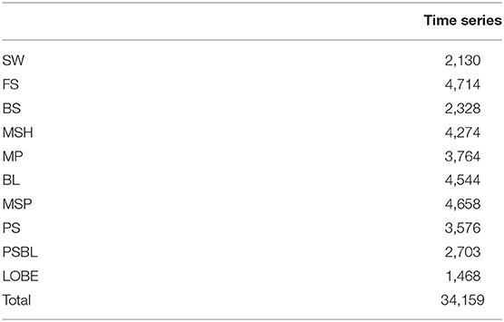
Table 2. Number of occurrences for each class.

This operation yields a dataset as an multidimensional array of size (34159, 40, 12). Finally, to input this array to the TSC model (and to avoid temporal bias due to the spacecraft orbit), we shuffle and randomly split the time series into training (56.25%), test (25%), and validation (18.75%) datasets. These three classical categories are defined such as:

• The training set is used to determined the weights of the model;

• The validation set is an out-of-sample set and allows to evaluate the error for data which has not been observed. In particular, the validation set is used for hyperparameter search and early stopping to avoid over-fitting ensuring a good generalization of the model;

• The test set is also an out-of-sample set which has not been used during training. The data are only used after the training to assess the performance of the final model, after training and hyperparameter optimization.

3. Classification Methods With a Fully Convolutional Neural Network

In this section, we overview the machine-learning algorithm we use: the fully convolutional neural network (FCN). This algorithm is assessed with several evaluation metrics. FCN works with time-dependant inputs (time series) in order to learn dynamical features. The main purpose of classifying time series and not only the instantaneous values is to learn automatically different features across the time dimension. The events can be characterized by dynamical insights at different scales learned by the model. We present a second model, called Multilayer perceptron (MLP), in the Supplementary Materials. It considers the input of the 12 variables as time independent. The main advantages of this method are its simplicity to prepare the machine learning pipeline and the possibility to work with any temporal resolution. However, the classification performance is much lower.

The FCN belongs to the category of artificial neural networks. They are usually characterized by their architecture: number of layers, type of connection (feedforward, feedback, convolution, etc.), and the activation functions. A layer is defined as a set of neurons which are not connected to each other. We selected neural network as they are able to learn non-linear models and can handle large datasets compared to kernel methods.

3.1. Model Presentation

Time series classification (TSC) is an active field of research and hundreds of different algorithms have been developed in recent years (Bagnall et al., 2017). Classical TSC usually uses new features spaces generated from the time series. The best performing models can combine dozen of different classifiers and feature transformations, leading to significant complexity and an important computational cost (Lucas et al., 2019).

Even if deep learning has seen very successful applications in the last decades, only a few examples of algorithms for TSC exist. This lack of overview has been filled recently (Fawaz et al., 2019) and several models show very promising results. In particular, we are convinced that convolution architectures can build very accurate classifiers. The convolutional layers use convolution in place of general matrix multiplication.

Local groups of values are often highly correlated in time series and they form distinctive local motifs that are easily detected. Convolutional layers are designed to identify these patterns invariant to location: if a motif specific to a label appears in one part of the time series, it could also appear anywhere. Hence a convolutional layer sharing the same weights at different locations can detect temporal patterns in different parts of the time series (LeCun et al., 2015). Moreover, several deep learning frameworks, such as Tensorflow (Abadi et al., 2016) or Pytorch (Paszke et al., 2019), are nowadays freely available. They provide differentiable programming to build very efficient neural networks. Thus, we consider deep learning for TSC for these two reasons: the availability of high-quality frameworks and the relevance of convolutional architectures.

The Fully Convolutional Network (FCN) (Wang et al., 2017) is a competitive deep-learning architecture for TSC yielding good results on large benchmarks (Fawaz et al., 2019). The network architecture is relatively simple and is comprised of a sequence of thee time convolution blocks followed by a global average pooling block (Lin et al., 2013). Each time convolution block is divided into a convolution layer, a batch normalization layer, and a Rectified Linear Unit (RELU) Nair and Hinton (2010) activation function. The convolutional layer is used to extract temporal features from the inputs by performing a convolution between the input signal and several filters. Each convolutional block has different filter lengths in order to analyze several time scales. The extracted features of the last convolutional block are used as inputs for the global average pooling (GAP) module to output the classification result. This last block is composed of the global average pooling layer and the Softmax layer. A more complete description of the FCN architecture can be found in Wang et al. (2017) and Fawaz et al. (2019).

As regards the numerical parameter, we performed a bayesian optimization to select the hyperparameters using the validation set for four parameters:

• The optimizer: adam or rmsprop

• The learning rate: between 10⁻⁶ and 10⁻³;

• The batch size: 32, 64, or 92;

• The number of filters: the baseline of the FCN paper, half the baseline and twice the baseline. The baseline given by the FCN paper (Wang et al., 2017) is the following: the first convolutional block has 128 filters with a filter length equal to 8, the second convolution extracts features with 256 filters of size 5 and the final convolutional layer is defined by 128 filters, each one with a length equal to 3.

The final FCN is trained for 1, 000 epochs with the categorical cross entropy as loss function. The result of the bayesian optimization provides the different hyperparameters. The Adam optimizer is used with an initial value of the learning rate set to 0.00002. An adaptive learning rate decrease is selected (with a minimum learning rate of 10⁻⁶), reducing the learning rate when the validation accuracy has stopped improving for 50 epochs. A batch size of 92 is used with twice the baseline configuration for the number of filters. The final FCN has 1, 079, 000 free parameters. The method of early termination is adopted to avoid over-fitting and stops the learning process when the validation loss did not decrease for 20 epochs. All the time series are standardized before the training process. The learning curve is presented in Figure 1. The learning process stopped after 140 epochs thanks to the early termination strategy.

FIGURE 1

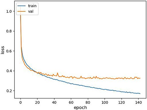
Figure 1. Learning curve history comparing training and validation loss.

3.2. Performance Evaluation

Assessing accurately the quality of a classification model raises significant challenges. A single and unified performance metric cannot effectively evaluate a multi-class classifier from all perspectives, such as class-balance or the number of different outcomes. Therefore, several metrics generalized from binary classification are considered.

The confusion matrix is a basic but useful tool to visualize the distribution of the predicted classes. Each column of the matrix gives the instances of a true class while each row represents the instance of a predicted class. Several metrics from binary classification can be generalized to multiclass by considering the prediction of each class as a binary classification problem: the given class has been predicted (positive) or not (negative). Then, the total number of True Positive (TP), True Negative (TN), False Positive (FP), and False Negative (FN) can be computed and several metrics are defined:

- Accuracy is the most intuitive metric and gives the percentage of correct predictions among all the predictions N_p:

$\begin{array}{ll}accuracy=\frac{TP+TN}{N_p}.& (1)\end{array}$

- Precision, also called positive predictive value, measures the proportion of positive values that are correctly identified as such among all predicted positives. In other words, it corresponds to the percentage of detections that are right. High precision is associated to a small amount of FP:

$\begin{array}{ll}precision=\frac{TP}{TP+FP}.& (2)\end{array}$

- Recall, also called the true positive rate, measures the proportion of positives detected. A significant number of missed true values (FN) leads to low recall:

$\begin{array}{ll}recall=\frac{TP}{TP+FN}.& (3)\end{array}$

- F1-score is the harmonic mean of precision and recall. Usually, high recall is detrimental to precision and vice versa. Therefore, the F1-score gives a trade-off between the two quantities and can help to compare two classifiers with different precision and recall values:

$\begin{array}{ll}accuracy=2.\frac{precision.recall}{precision+recall}.& (4)\end{array}$

All these metrics are computed for each class. Therefore, averaged quantities can be also defined to provide a more general view of the classifier. A macro-average gives the unweighted mean of the metric without taking imbalance into account and a micro-average computes the average weighted by the number of true instances for each class. The micro-average will account for label imbalance.

Finally, a receiver operating characteristic (ROC), also called ROC curve, is a graphical tool illustrating the performance of a binary classifier system when the discrimination threshold is varied. Indeed, each class prediction is associated to a probability. Usually, the class predicted by the classifier is chosen as the class with the highest probability. Instead, a threshold value can be used to decide if the class is effectively predicted by the classifier. The ROC curve plots the fraction of true positives out of all the predicted positives (True Positive Rate) vs. the fraction of false positives out of all the predicted negatives (False Positive rate) at various threshold values. For instance, all classes are predicted with a zero threshold (False Positive Rate and True Positive Rate of 1.0) while there are no correct predicted class and no false positive with a unit threshold (False Positive Rate and True positive rate of 0.0). A perfect classifier is located on the left corner of the curve with a true positive rate of 1.0 and a false positive rate of 0.0. A ROC curve can be drawn for each class. In case of a model with no discrimination capacity to distinguish between positive class and negative class, the ROC curse is a straight line of slope 1. The area under the ROC curve (AUC) summarized in one number if the model is capable of distinguishing between classes.

4. Results

4.1. Classification of MMS Data

We use here the test set (the out-of-sample set that is not involved in the training process) to evaluate the performance of the model. It is obtained by shuffling 25% of the data as described in section 2.3.

Table 3 summarizes the precision, recall, f1-score, and AUC evaluated by the FCN for the 10 different classes. In term of absolute values, the FCN shows great performance metrics. The AUC value is above 0.98 for all the classes. It means that a significant probability is always associated to the correct region by the classifier, even it is not the highest probability. For instance, the classifier could give a probability of 45% to the SW and 35% to the FS for a test sample belonging to the FS. Even if the prediction is wrong, the classifier still has detected some features which can belong to the correct class.

TABLE 3

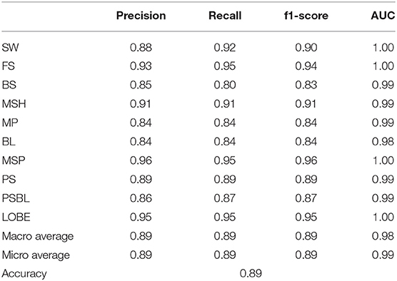
Table 3. Classification report for FCN computed on the test set.

Two different groups of regions are identified in Table 3. The first group consisting of the FS, the MSP, and the LOBE is very well-predicted with a respective f1-score above 0.94 and a AUC of 1.00. Such regions show usually very specific patterns, explaining why the classification metrics are very high. The second group is formed by the BS, the MP, the BL, the PS, and the PSBL, with smaller metric values, such as a f-1 score between 0.82 and 0.88 and a AUC between 0.98 and 0.99. Figure 2 shows the different ROC curves for the FCN. BL and BS are the lowest curves. They have a much higher false positive rate when they reached a true positive rate of 1.0 compared to the other classes. It means that, for some very specifics predictions, the classifier associates a very low probability to the correct class. The BL and the BS are thin regions marking the boundary between larger regions. Therefore, several time intervals labeled by SITLs may overlap two or more nearby regions. It could explain the lower metric values for these two regions.

FIGURE 2

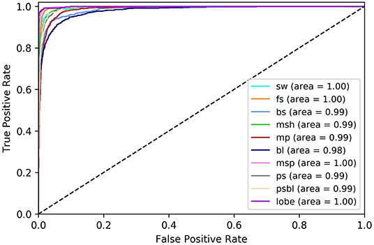
Figure 2. Receiver operating characteristic curve computed on the test set.

From the Supplementary Material, the second model (MLP) has important also problems to classify regions with strong variations, such as the BS with a f-1 score below 0.5. Thus, it seems that convolutional methods help to improve the accuracy of the classifier for the most challenging regions and it validates the choice of such algorithms designed to extract important temporal features and variations.

Table 4 gives details on the FCN predictions with a confusion matrix. Very typical errors can be observed for nearby regions, such as: SW and FS; PS, BL, and PSBL; PSBL and LOBE; MP, MSH and BL. These errors can be explained by physical arguments. The plasma properties can be similar for several nearby regions. For instance, we may expect that MP shares common properties with MSH and MSP as the MP acts as a boundary between the two other regions. The SW region can also be very similar to the FS as the latter comes from the reflection of the SW on the BS, as stated in the introduction. Therefore, it may be concluded that the FCN model really learned the typical patterns associated to each region as the main errors are identified for regions with similar physics.

TABLE 4

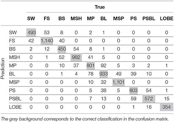
Table 4. Confusion Matrix for FCN computed on the test set.

4.2. Examples of MMS Classification

In this section, we show some examples of time series observed by the MMS spacecraft as it spanned the different near-Earth regions, along with the labels of the classifications made by the FCN model.

Figure 3 shows the MMS1 probe observations for the whole day of 2019-11-09, during which it flew through the dayside region. From top to bottom, the figure panels show the energy spectrum of the omnidirectional ion flux, the three components of the magnetic field (B_x, B_y, B_z) in GSE coordinates and its magnitude B_tot, the ion number density, the three components of the ion bulk velocity (V_x, V_y, V_z) in GSE coordinates, the ion temperatures parallel and perpendicular (T_∥, T_⊥) to the ambient magnetic field, and finally the labels given by the FCN model (FCN labels). The time in UT format and the spacecraft position (X_pos, Y_pos, Z_pos in R_E and GSE coordinates) are displayed at the bottom of the X-axis.

FIGURE 3

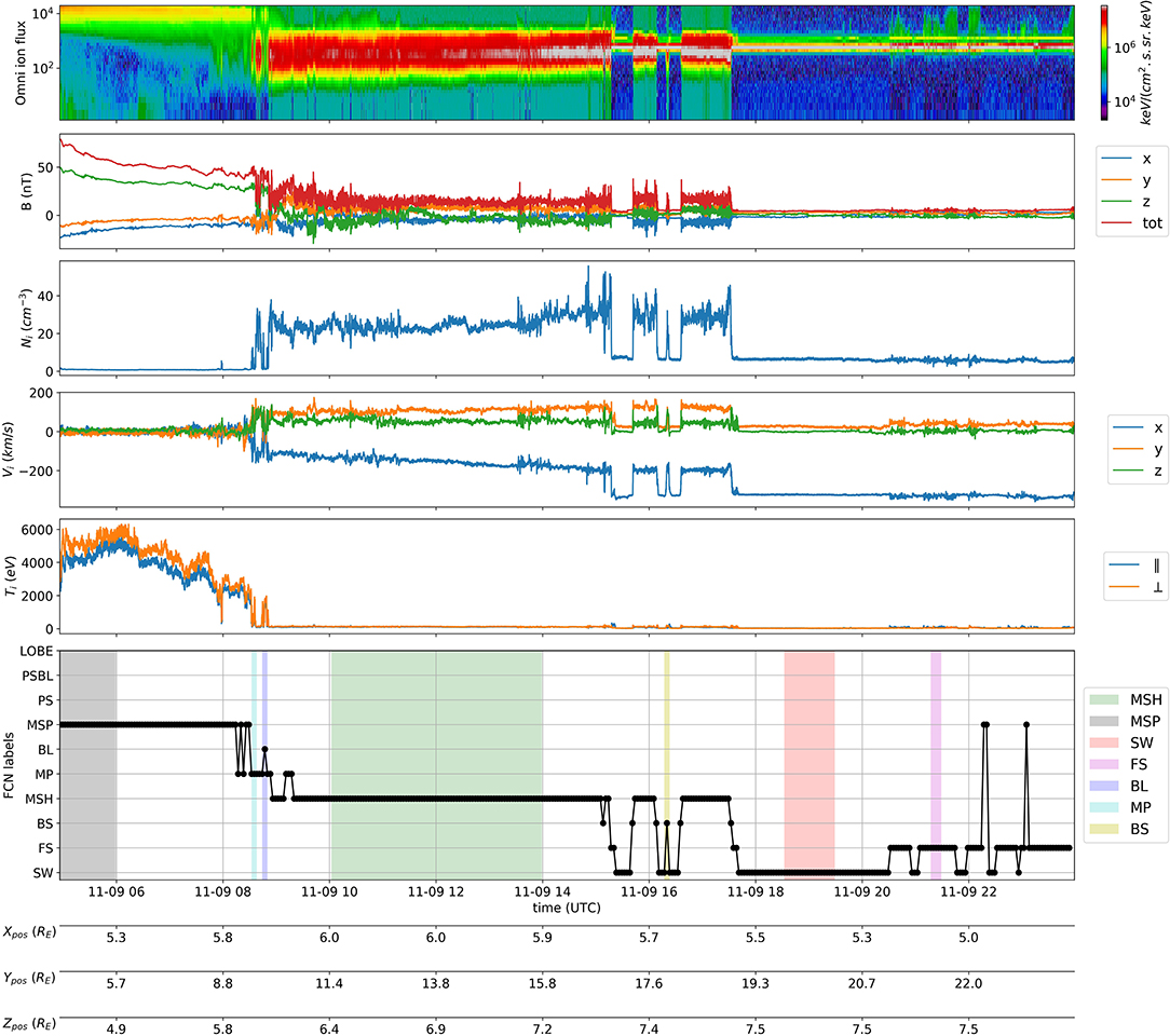
Figure 3. Example of MMS dayside classification. Labels, not present in the initial data set, have been manually added to compare the FCN predictions with a ground truth. They are represented by colored regions on the FCN labels plot.

In this example, the FCN model classifies well the regions, as its labels follow to a great extend the MMS1 observations: first the spacecraft is located in the magnetosphere, then it crosses the magnetopause to enter the magnetosheath, afterwards it flies through a series of bow shocks and goes back and forth to the solar wind, until it finally enters the solar wind. The model is even able to precisely detect the small-scale dynamics of the boundary regions such as partial magnetopause, boundary layer and bow shock crossings, and the come and go between the solar wind and the ion foreshock. Only three points seem to be clearly misclassified (as MSP) in the ion foreshock. However, these points can be easily eyeballed as outliers or discriminated by their low quality flag.

Figure 4 shows another example of the FCN classification method described above, but this time when MMS spacecraft flew through the nightside region. The MMS1 observations take place during the whole day of 2019-07-13, and the format is the same as in Figure 3. In this example again, the FCN model is able to label properly the regions spanned by MMS1: at the very beginning MMS1 exits the magnetosphere to the plasma sheet boundary layer, then goes in and out the lobe regions before reaching the plasma sheet. Again, the FCN model is also able to pick up the small-scale dynamics such as short plasma sheet crossings.

FIGURE 4

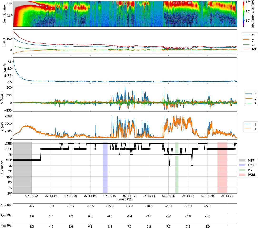
Figure 4. Example of MMS nightside classification. Labels, not present in the initial data set, have been manually added to compare the FCN predictions with a ground truth. They are represented by colored regions on the FCN labels plot.

The two examples shown in this section therefore support the good metrics obtained in the previous section, showing concretely that the FCN model is suited to properly label most of the MMS data with the regions spanned.

4.3. Locating Important Feature in Time Series With Class Activation Map

Class Activation Map (CAM) is a technique developed by Zhou et al. (2016) to get the discriminative regions used by a CNN to identify a specific class in the input data. I. CAM has been applied to TSC for one-dimensional case in Wang et al. (2017) for the first time. The objective in our case is to highlight the subsequences (i.e., sections) in each time series which are relevant to its class. Thus, this approach allows to explain the decision taken by the classifier. The mathematical description of the method can be found in Zhou et al. (2016), Wang et al. (2017), and Fawaz et al. (2019). This method works only for models with the global average pooling as last layer (Lin et al., 2013). CAM is represented by a univariate time series (with the same size than the FCN input) where the value gives the importance of the signal to classification. Low values mean the subsequence does not contribute to the decision of the classifier while high values mean the section contributes significantly.

Figure 5 shows CAM examples for two different classes: the solar wind and the foreshock. For each class, a well-predicted time series is drawn and colored by the value of the CAM, illustrating the results from MMS data given in section 4.1. As regards the SW example, almost all the input signal contributes to the classification, as stated by the uniform CAM values above 0.8 between 20 and 160 s. It means that the values of input features are much more important than their variations or than specific patterns. On the other hand, the classifier detects the FS mainly thanks to a specific pattern around 65 s associated to extrema for B_x, B_y, N_i, and V_y and significant slopes for the other features. Only a few specific time intervals are involved in the decision of the classifier for FS. The CAM analysis strengthens the conclusion that temporal and dynamical analysis are fundamental to classify nearby regions with fluctuating behaviors. For instance, the MLP results given in the Supplementary Materials shows that a significant number of SW region are misclassified as FS as the model works only on instantaneous quantities.

FIGURE 5

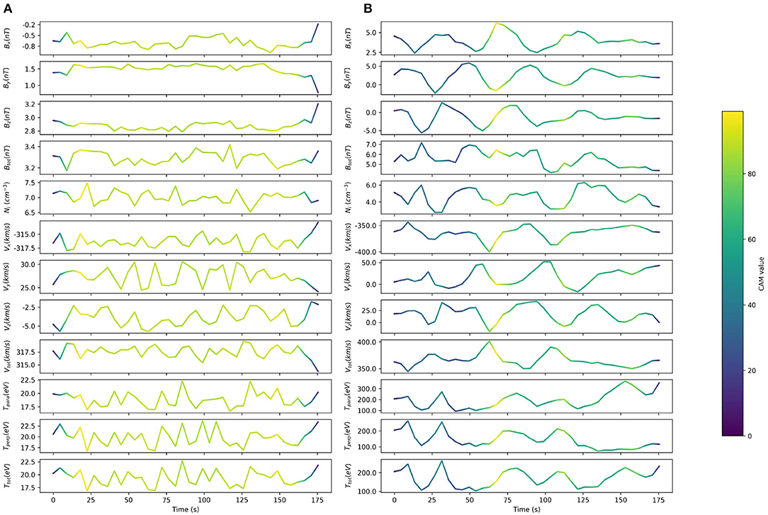
Figure 5. The Class Activation Map highlighting the important sections of the time series contributing most to the classification. Low values mean the time step of the time series does not contribute to the decision of the classifier while high values mean the time step contributes significantly. (A) Solar wind. (B) Foreshock.

4.4. Extension to Cluster Mission

In this section, we put to test the adaptability of the FCN model to different magnetospheric data, namely data from the Cluster mission. This mission has been chosen as the data is pretty close to MMS data (notably the data sampling), and a 2-year period of labeled data is available (see Nguyen et al., 2019) to audit the classification resulting from the model.

First, we qualitatively assess the quality of the different classification methods, by comparing them with C1 probe observations. We randomly select a day during which the C1 probe flew through the dayside region. This example, from the day of 2005-02-13, is shown in Figure 6 in the same format as Figures 3, 4, except that we include the manual labels from Nguyen et al. (2019) (named “Man labels”) in the penultimate bottom panel.

FIGURE 6

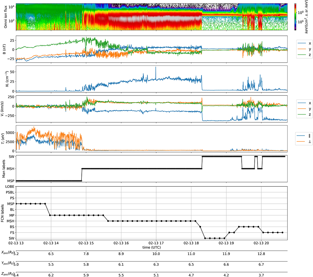
Figure 6. Example of Cluster dayside classification.

The “Man labels” are in good agreement with the observations of C1, as the probe is first located in the magnetosphere, then flies through the magnetosheath and finally reaches the solar wind. The “FCN labels” show also good agreement with C1 observations: the probe is first located in the magnetosphere and then crosses the magnetopause a few times before entering the magnetosheath, then it crosses the bow shock to enter the solar wind before crossing several times again the bow shock and finally spanning the ion foreshock. As in the examples shown for the MMS mission, the FCN model is able to pick up the small-scale dynamics of the near-Earth frontiers: the magnetopause, the bow shock and the foreshock. As a result, the model is able to outperform the manual labels by identifying in more detail the magnetospheric regions, in particular the small-scale dynamics of the transition regions.

Then, we take advantage of the 2-year period of Cluster labeled data from Nguyen et al. (2019) to quantify the quality of the FCN model classification, by investigating the performance metrics. We select the points labeled as “MSP,” “MSH,” and “SW” by the FCN model using Cluster data from the 2005–2006 period, and compare them with the labels for these 3 regions obtained from Nguyen. Using this method, we obtain an accuracy classification score of 0.97 over a total of 10, 929 common labeled points. the classification report can be found in Table 5. We note here that this score is not an exact quantization of the model's accuracy on Cluster data, and the classification score is probably overestimated because only 3 classes (i.e., magnetospheric regions) are considered here instead of the 10 included in the FCN model. Therefore, a dataset of Cluster data labeled with these 10 near-Earth regions is required to get an absolute quantification of its accuracy regarding the Cluster mission. However, it shows globally that our FCN model classification is a reliable method for the labeling of the Cluster mission data and potentially other heliophysics missions.

TABLE 5

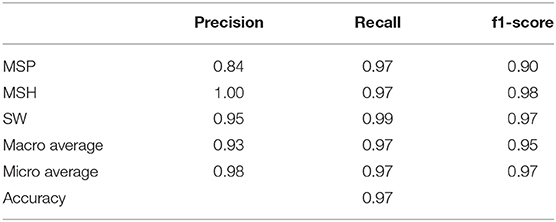
Table 5. Classification report for FCN computed on the Cluster dataset.

4.5. Resources

The most time-consuming task in the present work has been the data preparation and the parsing of the SITL reports. Training a FCN model needs about 200 CPU hours on a workstation featured with an Intel Xeon E5-2670 v3 (12 cores at 2.30 GHz). These values must be multiplied by the number of different trials needed to optimize the hyperparameters (about 40 in that case).

5. Discussion and Conclusions

Using deep learning algorithms, namely a fully convolutional neural network (FCN), we built an automatic detection of 10 near-Earth regions: the solar wind, the ion foreshock, the bow shock, the magnetosheath, the magnetopause, the boundary layer, the magnetosphere, the plasma sheet, the plasma sheet boundary layer and the lobes.

Using more than 3 years of labeled (SITL and additional human-labeled) MMS mission data, we showed that this method are reliable to classify near-Earth regions. The FCN method(1,079,000 free parameters) has been very effective in taking into account the dynamical features of the most challenging plasma regions (important data variability due to the fluctuations of the plasma), in particular the bow shock and the boundary layer. The high accuracy of the FCN model also highlights the quality of the labeled data set generated from SITL reports. We demonstrate the good accuracy of the classification predictions on the test and validation datasets, but also on unlabeled data from the MMS mission. We also show the adaptability of the trained FCN model by applying the classification to the Cluster ESA mission data. The predictions showed good accuracy and enhanced dynamics in comparison with previous human-labeled dataset.

These results show on one hand that the model can be applied to the whole MMS dataset, which would be of great interest to map the different magnetospheric boundaries and build empirical models of the properties and dynamics of the plasma in the near-Earth space. On the other hand, these results show that the model could be applied on different space missions orbiting around Earth (such as Cluster or THEMIS) or other planets to automatically label available data. However, we recommend to build a small labeled dataset specific to each mission with limited retraining of the last layer. This process called transfer learning could help improving the generalization of our labeled dataset to other missions such as the JUICE mission, which will be launched in 2022 and for which selective downlink strategies are being discussed.

As a matter of fact, the model could be used as a support to the scientific experts in charge of the data selection process (such as the SITL system), providing classification of the regions that would contribute to ease and speed up this time-consuming and tedious task. Such lightweight and easily-adaptable algorithms could also be important for the so-called SOC (Science Operation Center) of current and future spacecraft missions, both on ground and onboard. For the latter case, these algorithms could be implemented within onboard spacecraft digital boards to automatically select regions and events of scientific interest, much reducing the complexity and the cost of science operations.

The intended integration of this model into the aidapy package², which allows to automatically load selected data from open-access databases, will be of particular interest by providing plasma data accompanied with region labels and quality flags on the fly for use case and statistical studies. The integration of such lightweight algorithms can be also generalized to other programs.

In terms of modeling, we expect to improve the FCN results by generalizing the use of hyperparameter optimization for a higher number of hyperparameters and on larger ranges. We also plan to investigate the use of convolution methods directly on the omnidirectional ion energy fluxes.

Finally, the classification of near-Earth regions represents only a first step for the time series classification in heliophysics. It paves the way to more ambitious models, such as the identification and the classification of space plasma processes (e.g., magnetic reconnection and structures, waves and turbulence or plasma jets), as well as their combinations. However, this topic is beyond the scope of the present study and is left for a forthcoming study.

Data Availability Statement

The models used for this study, the post-processing tools, and the link to the data can be found in the Jupyter notebook classification results.ipynb in the AIDA repository³.

Author Contributions

HB and RD built the data set, the machine learning models and wrote the manuscript. HB, RD, AR, and OL gathered information from SITL reports and provided information for their usage for machine learning. HB, AR, OL, and GL provided physical interpretation of the results. RD and JA provided insights into the use of the different machine learning techniques. AR and GL supervised the work. All authors contributed to manuscript revision, read, and approved the submitted version.

Funding

This paper has received funding from the European Unions Horizon 2020 research and innovation programme under grant agreement No. 776262 (AIDA, http://www.aida-space.eu).

Conflict of Interest

The authors declare that the research was conducted in the absence of any commercial or financial relationships that could be construed as a potential conflict of interest.

The reviewer JB declared a past co-authorship with one of the authors AR to the handling editor.

Acknowledgments

Data were retrieved using HELIOPY v0.5.3 (Stansby et al., 2020) and processed using aidapy⁴, pandas McKinney (2010), and scikit-learn (Pedregosa et al., 2011). Figures were produced using matplotlib (Hunter, 2007). The model has been built with Keras from Tensorflow 2.2 (Abadi et al., 2016) and we modified scripts provided in the dl-4-ts repository⁵. The hyperparameter optimization is performed with the Python library optuna (Akiba et al., 2019). The authors would like to acknowledge Gautier Nguyen (LPP) for providing classifications on Cluster data, Nicolas Aunai (LPP) and Alexis Jeandet (LPP) for the helpful discussion and support.

Supplementary Material

The Supplementary Material for this article can be found online at: https://www.frontiersin.org/articles/10.3389/fspas.2020.00055/full#supplementary-material

Footnotes

1. ^https://gitlab.com/aidaspace/aidapy

2. ^https://gitlab.com/aidaspace/aidapy

3. ^https://gitlab.com/aidaspace/notebooks_aida/-/tree/master/04_sitl_classification_region

4. ^https://gitlab.com/aidaspace/aidapy

5. ^https://github.com/hfawaz/dl-4-tsc

References

Abadi, M., Barham, P., Chen, J., Chen, Z., Davis, A., Dean, J., et al. (2016). “Tensorflow: a system for large-scale machine learning,” in 12th USENIX Symposium on Operating Systems Design and Implementation (OSDI 16) (Savannah, GA), 265–283.

Google Scholar

Akiba, T., Sano, S., Yanase, T., Ohta, T., and Koyama, M. (2019). “Optuna: a next-generation hyperparameter optimization framework,” in Proceedings of the 25th ACM SIGKDD International Conference on Knowledge Discovery & Data Mining (Anchorage, AK), 2623–2631. doi: 10.1145/3292500.3330701

CrossRef Full Text | Google Scholar

Argall, M. R., Small, C., Piatt, S., Breen, L., Petrik, M., Barnum, J., et al. (2020). MMS SITL ground loop: automating the burst data selection process. arXiv [Preprint]. arXiv:2004.07199. doi: 10.3389/fspas.2020.00054

CrossRef Full Text | Google Scholar

Bagnall, A., Lines, J., Bostrom, A., Large, J., and Keogh, E. (2017). The great time series classification bake off: a review and experimental evaluation of recent algorithmic advances. Data Mining Knowl. Discov. 31, 606–660. doi: 10.1007/s10618-016-0483-9

PubMed Abstract | CrossRef Full Text | Google Scholar

Balasis, G., Aminalragia-Giamini, S., Papadimitriou, C., Daglis, I. A., Anastasiadis, A., and Haagmans, R. (2019). A machine learning approach for automated ULF wave recognition. J. Space Weather Space Clim. 9:A13. doi: 10.1051/swsc/2019010

CrossRef Full Text | Google Scholar

Balogh, A., Carr, C. M., Acuña, M. H., Dunlop, M. W., Beek, T. J., Brown, P., et al. (2001). The Cluster Magnetic Field Investigation: overview of in-flight performance and initial results. Ann. Geophys. 19, 1207–1217. doi: 10.5194/angeo-19-1207-2001

CrossRef Full Text | Google Scholar

Baumjohann, W., and Treumann, R. A. (1996). Basic Space Plasma Physics. London: Imperial College Press. doi: 10.1142/p015

CrossRef Full Text | Google Scholar

Burch, J., Moore, T., Torbert, R., and Giles, B. (2016). Magnetospheric multiscale overview and science objectives. Space Science Reviews, 199(1-4):5-21. doi: 10.1007/s11214-015-0164-9

CrossRef Full Text | Google Scholar

Camporeale, E., Caré, A., and Borovsky, J. E. (2017). Classification of solar wind with machine learning. J. Geophys. Res. Space Phys. 122, 10–910. doi: 10.1002/2017JA024383

CrossRef Full Text | Google Scholar

Dungey, J. W. (1963). Interactions of solar plasma with the geomagnetic field. Planet. Space Sci. 10, 233–237. doi: 10.1016/0032-0633(63)90020-5

CrossRef Full Text | Google Scholar

Esling, P., and Agon, C. (2012). Time-series data mining. ACM Comput. Surv. 45, 1–34. doi: 10.1145/2379776.2379788

CrossRef Full Text | Google Scholar

Fawaz, H. I., Forestier, G., Weber, J., Idoumghar, L., and Muller, P.-A. (2019). Deep learning for time series classification: a review. Data Mining Knowl. Discov. 33, 917–963. doi: 10.1007/s10618-019-00619-1

CrossRef Full Text | Google Scholar

Hunter, J. D. (2007). Matplotlib: a 2D graphics environment. Comput. Sci. Eng. 9, 90–95. doi: 10.1109/MCSE.2007.55

CrossRef Full Text | Google Scholar

Jelínek, K., Němeček, Z., and Šafránková, J. (2012). A new approach to magnetopause and bow shock modeling based on automated region identification. J. Geophys. Res. Space Phys. 117:A05208. doi: 10.1029/2011JA017252

CrossRef Full Text | Google Scholar

Kivelson, A., Kivelson, M., and Russell, C. (1995). Introduction to Space Physics. Cambridge University Press. doi: 10.1017/9781139878296

CrossRef Full Text | Google Scholar

LeCun, Y., Bengio, Y., and Hinton, G. (2015). Deep learning. Nature 521, 436–444. doi: 10.1038/nature14539

PubMed Abstract | CrossRef Full Text | Google Scholar

Lin, M., Chen, Q., and Yan, S. (2013). Network in network. arXiv [Preprint]. arXiv:1312.4400.

Google Scholar

Lucas, B., Shifaz, A., Pelletier, C., O'Neill, L., Zaidi, N., Goethals, B., et al. (2019). Proximity forest: an effective and scalable distance-based classifier for time series. Data Mining Knowl. Discov. 33, 607–635. doi: 10.1007/s10618-019-00617-3

CrossRef Full Text | Google Scholar

McKinney, W. (2010). “Data structures for statistical computing in Python,” in Proceedings of the 9th Python in Science Conference (Austin, TX), 56–61. doi: 10.25080/Majora-92bf1922-00a

CrossRef Full Text | Google Scholar

Nair, V., and Hinton, G. E. (2010). “Rectified linear units improve restricted Boltzmann machines,” in Proceedings of the 27th International Conference on Machine Learning (ICML-10) (Haifa), 807–814.

Google Scholar

Nguyen, G., Aunai, N., Michotte de Welle, B., Jeandet, A., and Fontaine, D. (2019). Automatic detection of the earth bow shock and magnetopause from in-situ data with machine learning. Ann. Geophys. Discuss. 2019, 1–22. doi: 10.5194/angeo-2019-149

CrossRef Full Text | Google Scholar

Nishizuka, N., Sugiura, K., Kubo, Y., Den, M., Watari, S., and Ishii, M. (2017). Solar flare prediction model with three machine-learning algorithms using ultraviolet brightening and vector magnetograms. Astrophys. J. 835:156. doi: 10.3847/1538-4357/835/2/156

CrossRef Full Text | Google Scholar

Olshevsky, V., Khotyaintsev, Y. V., Divin, A., Delzanno, G. L., Anderzen, S., Herman, P., et al. (2019). Automated classification of plasma regions using 3d particle energy distribution. arXiv [Preprint]. arXiv:1908.05715.

Google Scholar

Paszke, A., Gross, S., Massa, F., Lerer, A., Bradbury, J., Chanan, G., et al. (2019). “PyTorch: an imperative style, high-performance deep learning library,” in Advances in Neural Information Processing Systems 32, eds H. Wallach, H. Larochelle, A. Beygelzimer, F. d'Alché-Buc, E. Fox, and R. Garnett (Curran Associates, Inc.), 8026–8037. Available online at: http://papers.nips.cc/paper/9015-pytorch-an-imperative-style-high-performance-deep-learning-library.pdf

Google Scholar

Pedregosa, F., Varoquaux, G., Gramfort, A., Michel, V., Thirion, B., Grisel, O., et al. (2011). Scikit-learn: machine learning in Python. J. Mach. Learn. Res. 12, 2825–2830. Available online at: https://dl.acm.org/doi/10.5555/1953048.2078195

Google Scholar

Pollock, C., Moore, T., Jacques, A., Burch, J., Gliese, U., Saito, Y., et al. (2016). Fast plasma investigation for magnetospheric multiscale. Space Sci. Rev. 199, 331–406. doi: 10.1007/s11214-016-0245-4

CrossRef Full Text | Google Scholar

Rème, H., Aoustin, C., Bosqued, J. M., Dandouras, I., Lavraud, B., Sauvaud, J. A., et al. (2001). First multispacecraft ion measurements in and near the Earth's magnetosphere with the identical Cluster ion spectrometry (CIS) experiment. Ann. Geophys. 19, 1303–1354. doi: 10.5194/angeo-19-1303-2001

CrossRef Full Text | Google Scholar

Russell, C., Anderson, B., Baumjohann, W., Bromund, K., Dearborn, D., Fischer, D., et al. (2016). The magnetospheric multiscale magnetometers. Space Sci. Rev. 199, 189–256. doi: 10.1007/s11214-014-0057-3

CrossRef Full Text | Google Scholar

Stansby, D., Rai, Y., Argall, M., JeffreyBroll Erwin, N., Shaw, S., et al. (2020). heliopython/heliopy: Heliopy 0.10.0. Available online at: https://zenodo.org/record/3676651#.Xz38LSgzaUk

Google Scholar

Torbert, R., Russell, C., Magnes, W., Ergun, R., Lindqvist, P.-A., LeContel, O., et al. (2016). The fields instrument suite on MMS: scientific objectives, measurements, and data products. Space Sci. Rev. 199, 105–135. doi: 10.1007/s11214-014-0109-8

PubMed Abstract | CrossRef Full Text | Google Scholar

Wang, Z., Yan, W., and Oates, T. (2017). “Time series classification from scratch with deep neural networks: a strong baseline,” in 2017 International Joint Conference on Neural Networks (IJCNN) (Anchorage, AK: IEEE), 1578–1585. doi: 10.1109/IJCNN.2017.7966039

CrossRef Full Text | Google Scholar

Zhou, B., Khosla, A., Lapedriza, A., Oliva, A., and Torralba, A. (2016). “Learning deep features for discriminative localization,” in Proceedings of the IEEE Conference on Computer Vision and Pattern Recognition (Las Vegas, NV), 2921–2929. doi: 10.1109/CVPR.2016.319

CrossRef Full Text | Google Scholar