Variability of Gravity Wave Effects on the Zonal Mean Circulation and Migrating Terdiurnal Tide as Studied With the Middle and Upper Atmosphere Model (MUAM2019) Using a Nonlinear Gravity Wave Scheme

1. Introduction

Atmospheric gravity waves (GW) are known to cause a variety of effects in the middle and upper atmospheres of Earth (e.g., Hines, 1960; Richmond, 1978; Taylor et al., 1998; Fritts and Alexander, 2003; Snively and Pasko, 2003; Yue et al., 2009; de la Torre et al., 2014; Becker and Vadas, 2020) and all planetary atmospheres that have been studied so far (e.g., Creasey et al., 2006a; Creasey et al., 2006b; Parish et al., 2009; Medvedev et al., 2011; Miyoshi et al., 2011; Spiga et al., 2012; Walterscheid et al., 2013; Yiğit and Medvedev, 2019). Historically, the importance of GWs for atmospheric dynamics has been acknowledged first in the context of Earth’s middle atmosphere (e.g., Holton, 1982). For about 2 decades later, it has been widely assumed that GW effects are confined to the mesosphere. However, a number of studies, especially since the second half of 2000s, have shown that GW effects extend well into the thermosphere (e.g., Vadas and Fritts, 2004; Vadas, 2007; Hickey et al., 2009; Yiǧit et al., 2009; Yiğit and Medvedev, 2010; Fritts and Lund, 2011; Heale et al., 2014; Miyoshi et al., 2014; Gavrilov and Kshevetskii, 2015; Becker and Vadas, 2020), while coordinated observations also demonstrate thermospheric GW signatures (e.g., Park et al., 2014; Forbes et al., 2016; Trinh et al., 2018) that cannot be explained by considering solely solar and magnetic effects. Meanwhile, GWs are acknowledged as an important physical mechanism that contributes to the vertical coupling in the atmosphere-ionosphere system as has been discussed in contemporary reviews (e.g., Hocke and Schlegel, 1996; Nicolls and Heinselman, 2007; Nicolls et al., 2014; Yiǧit and Medvedev, 2015). During transient events such as sudden stratospheric warmings, thermospheric effects of GWs can be extremely variable depending on the nature of the warming (Yiğit and Medvedev, 2016; Nayak and Yiğit, 2019). Often, simple linear-type leave space GW parameterizations with ad hoc cut-off levels in the upper mesosphere and lower thermosphere have been used (e.g. Hines, 1960; Lindzen, 1981; McFarlane, 1987) in order to represent small-scale GWs not captured in coarse-grid general circulation models (GCMs). However, recent progress in GW dynamics suggests that GW schemes based on more accurate physics of GW dissipation are required in order to adequately represent subgrid-scale GW processes in GCMs (Yiǧit et al., 2008; Senf and Achatz, 2011; Heale et al., 2020). The recent progress of technology accompanied by increasing computer power even allows for the GW resolving models that are able to reproduce secondary and tertiary GWs (e.g., Liu et al., 2014; Becker and Vadas, 2020). However, for mechanistic models with limited resources, the scheme by Yiǧit et al. (2008) is the one that is most state-of-the-art.

A broad spectrum of internal waves exists in the atmosphere. While GWs have relatively small scales with respect to the planetary radius, solar tides are large-scale waves with horizontal wavelengths comparable to Earth’s radius. The most predominant types of atmospheric tides are the migrating diurnal (DTs), semidiurnal (SDTs), and the terdiurnal tides (TDTs). Despite the large differences in scales between the GWs and tides, they continuously interact with each other, potentially producing secondary tidal waves, which can then influence the upper atmosphere (Forbes et al., 1991; Miyahara and Forbes, 1991; Manson et al., 2002; Senf and Achatz, 2011; Vadas et al., 2014; Yiǧit and Medvedev, 2017; Lilienthal et al., 2018; Lilienthal and Jacobi, 2019). However, owing largely to the complexity of the interaction processes, there is an ongoing discussion about how GWs influence the solar tides. While significant amount of work has been dedicated to the relation between GWs, DTs, and SDTs (e.g., Liu et al., 2014; Becker, 2017; Yiǧit and Medvedev, 2017; Baumgarten et al., 2018; Trinh et al., 2018), the progress on the understanding of the interaction between GWs and the TDTs is relatively limited. Also, the vast majority of the studies focus on the MLT region in the context of GW–tide interactions. For example, using a numerical model of the DT coupled with simplified linear GW drag calculations, including only slow GW phase speeds, Miyahara and Forbes (1991) demonstrated that GW drag damps the tidal amplitudes in the MLT. The study by Manson et al. (2002), combining observations and a GCM, suggested that the tidal response highly depends on the type of the utilized GW parameterization. Using a ray tracing model, Ribstein and Achatz (2016) also came to the conclusion that such interactions strongly depend on model physics. Further model simulations by Lilienthal et al. (2018) and Lilienthal and Jacobi (2019) have shown that the GW–tide interactions can generate TDTs that can particularly be important for the dynamics of the lower thermosphere. However, they mainly focused on the variety and relative importance of forcing mechanisms of the TDT and did not analyze the zonal mean circulation in detail. Further, they rather used an incomplete representation of GW parameterization by coupling a linear Lindzen-type scheme for the lower and middle atmosphere and a nonlinear scheme based on Yiǧit et al. (2008) for the upper atmosphere. Coupling two different GW schemes can potentially produce limited insight into the kinematics of GWs. We have improved this aspect substantially in the current study. Overall, existing results on the GW–tide interactions all suggest that there is a distinct difference between linear and nonlinear GW schemes in terms of how they influence the solar tides. Undoubtedly, linear GW schemes provide only a limited picture of the actual GW dynamics in the atmosphere.

Various GW parameterizations have been developed so far (see reviews by Fritts and Alexander, 2003; Kim et al., 2003; Teixeira, 2014; Medvedev and Yiğit, 2019). The majority of these schemes have been designed for middle atmosphere GCMs. They have various advantages as well as assumptions and limitations. It is important to note that parameterization of GW source spectrum and propagation/dissipation are two separate challenges. The former is often called a source spectrum parameterization. The latter is based on some wave saturation theory. Among the source spectrum ones, some are designed exclusively for orographic GWs (McFarlane, 1987). Some schemes focus on convective generation of GWs in order to estimate the resulting wave fluxes at cloud top (Beres et al., 2004; Song and Chun, 2005). Other schemes focus on the propagation and processes through which waves saturate at higher levels (e.g., Lindzen, 1981; Warner and McIntyre, 2001; Yiǧit et al., 2008).

Our study is motivated by the recent progress in GW studies and the lack of knowledge concerning the nature of GW–tide interactions. Specifically, we implement for the first time a nonlinear GW parameterization (Yiǧit et al., 2008) into the middle and upper atmosphere model (MUAM) used at the University of Leipzig, Germany. In contrast to earlier MUAM versions, that used a rather outdated linear Lindzen-type GW scheme (based on Lindzen, 1981) with a cutoff in the lower thermosphere, the new scheme extends up to the thermosphere. We then study the interaction between the TDTs and GWs accounting for lower thermospheric GW effects in addition to the middle atmospheric effects.

The structure of the paper is as follows: The next section describes in detail the GCM, GW parameterization, and the simulations to be conducted. Section 3.1 presents the simulation results for the zonal mean fields based on the standard configuration of the GW scheme; Section 3.2 studies the effects of changing initial GW parameters; and Section 3.3 analyzes the interaction between GWs and the migrating TDT. Discussion and conclusions are given in Section 4.

2. Materials and Methods

2.1. Model Description

In the following experiments, we use the Middle and Upper Atmosphere Model (MUAM; Pogoreltsev, 2007; Pogoreltsev et al., 2007; Suvorova and Pogoreltsev, 2011), which is a three-dimensional mechanistic GCM solving the nonlinear primitive equations (e.g., Jakobs et al., 1986). The model is initialized with a windless atmosphere and a globally uniform standard temperature profile (Pogoreltsev et al., 2007), where the temperature profile above 130 km is constant. The 1,000 hPa layer is the lower boundary of MUAM based on 2000–2010 mean monthly mean ERA-Interim reanalysis fields (Dee et al., 2011) of the zonal mean temperature and geopotential height as well as the respective stationary planetary waves (SPWs) with wavenumbers 1–3 (see also Lilienthal et al., 2017). The horizontal resolution is 5° × 5.625° (latitudes $\times$ longitudes). There are 56 vertical levels, which are evenly spaced in logarithmic pressure height with p_s = 1,000 hPa as the reference pressure level and $H=7$ km as the scale height. Vertical spacing is about 2.8 km, and consequently, the upper boundary is located at $z_{56}\approx 160$ km. The lower levels up to 30 km height are nudged with 2000–2010 mean monthly mean ERA-Interim zonal mean temperature fields to correctly represent the dynamics in the lower atmosphere (Jacobi et al., 2015; Lilienthal et al., 2018). Solar and infrared radiative processes are parameterized according to Strobel (1978) and Fomichev and Shved (1985), respectively. These parameterizations focus on i) the absorption and emission processes of the most important atmospheric constituents like $H_{2}O$ (troposphere), $C{O}_2$ and $O_3$ (stratosphere) as well as on ii) absorption bands like the extreme ultra violet (EUV) band in the thermosphere. The $H_{2}O$, $C{O}_2$, and $O_3$ distributions are prescribed. Further parameterizations deal with thermospheric processes such as Rayleigh friction, ion drag, and Newtonian cooling.

Solar tides are generated self-consistently in the model by the absorption of solar radiation, mainly due to water vapor and ozone. Unlike other mechanistic models, there is no explicit tidal forcing at the lower boundary. The sources of TDTs within MUAM were demonstrated in the work by Lilienthal et al. (2018). These sources are predominantly solar heating in the troposphere and stratosphere, nonlinear interactions between the DT and SDT in the mesosphere, and GW-tide interactions in the thermosphere.

2.2. The Nonlinear Gravity Wave Parameterization

In contrast to earlier MUAM versions (e.g., Jacobi et al., 2006), where a linear, Lindzen-type GW scheme with multiple breaking levels was applied, we now use a nonlinear spectral whole atmosphere (tropopause to thermosphere) GW scheme according to the work by Yiǧit et al. (2008). Yiǧit et al. (2008) extensively compared the nonlinear whole atmosphere scheme to the Lindzen scheme and demonstrated the unphysical nature of the linear scheme. Without artificially reducing the GW drag, the Lindzen scheme produces very large GW drag, which is rather unrealistic and can potentially destabilize the model. The Lindzen scheme only works fine provided that an extensive amount of tuning is performed. Therefore, we updated our modeling framework with a more modern nonlinear GW parameterization that extends from the tropopause up to the thermosphere and whose physics and application have been discussed and tested in a number of previous publications (e.g., Yiǧit and Medvedev, 2017). An increasing number of whole atmosphere models are being developed, which further indicate the necessity of the use of GW schemes that are suitable for the whole atmosphere region. Note that MUAM is a mechanistic model with limited resources, suitable for case and sensitivity studies, presenting climatologies and not being a comprehensive Earth system model. Therefore, a GW resolving accuracy cannot be provided and we rely on standard GW parameterizations. This physical rationale and the detailed description of the scheme are given in a number of publications (e.g., Yiǧit et al., 2008; Yiğit and Medvedev, 2013; Miyoshi and Yiğit, 2019). It has been also used in studies of GW effects with Martian GCMs (e.g., Yiğit et al., 2018). Here we give a brief qualitative description.

GW dissipation occurs due to a combination of various dissipation processes, such as eddy viscosity, nonlinear wave–wave interactions (Medvedev and Klaassen, 2000), molecular diffusion and thermal conduction, and ion drag (Yiǧit et al., 2008; Yiǧit et al., 2009; Yiğit and Medvedev, 2010; Medvedev et al., 2017). In the MLT, the most dominant dissipation mechanism is due to the nonlinear interactions among the different GWs harmonics (Yiǧit et al., 2008). Eddy viscosity, for example, plays a relatively minor role in this context. Also, there is a significant degree of uncertainty in eddy viscosity in the MLT. Therefore, we decided to exclude the vertical profiles of the Newtonian cooling coefficient, the eddy diffusion coefficient and electron density in our implementation of the parameterization, i.e. these parameters are set to zero. The source level of GWs is defined near the tropopause at about 15 km similar to previous implementations of the whole atmosphere scheme (e.g., Yiğit et al., 2014; Yiǧit and Medvedev, 2017). Note that, despite most GWs originate in the troposphere, a lower launch level cannot provide better results in MUAM because the troposphere of MUAM is nudged. The model neither accounts for orography nor for deep convection. The GW spectrum specifies the GW momentum fluxes as a function of ground-based horizontal phase speeds. However, at the launch level, the asymmetric effects produced by the winds are taken into account. The vertical evolution of the wave momentum fluxes are significantly modified by the background winds. The details of source spectrum specification can be found in the papers mentioned above. Then, the present scheme describes the upward propagation of subgrid-scale GWs and their dissipation due to various realistic atmospheric dissipation processes mentioned above. Our GW scheme is not a parameterization of the GW sources. It relies on an empirical specification of the GW spectrum at an appropriate launch level. In principle, it can be coupled with other parameterizations of GW sources in the troposphere, if a given GCM can provide a self-consistent troposphere.

2.3. Experimental Setup

We first conduct a reference (benchmark) simulation, which will later facilitate an assessment of the changes induced by variations in the GW source spectrum. The benchmark case (called EXP1 hereafter) is generated by spinning up the model for a period of 390 days, in which the mean circulation is built up and different waves such as GWs (after day 60), planetary waves and tides (after day 180) are included. After the spin-up, we run the model for 30 days, which are used for our analysis of the background climatology (zonal/meridional wind and temperature) and wave parameters shown in Sections 3–5. Because MUAM is driven only by monthly mean boundary conditions and reaches almost a steady state with small day-to-day variations after the spin-up period, the average of these last 30 days represents the monthly mean state of the atmosphere.

For the GW spectrum of EXP1, we adapt the original spectrum by Yiǧit et al. (2008) who tested various spectral shapes. When the whole atmosphere GW scheme has been implemented into a GCM in the work by Yiǧit et al. (2009), the present GW source spectrum was validated and the authors found out that the utilized empirical source spectrum successfully reproduces the large-scale structure of the middle atmosphere dynamics. Therefore we use the original GW spectrum as the reference source spectrum in our current study. Note, however, that this spectrum is a representation of the mean behavior of global GW distribution. It is possible that it is underestimating the actual GW activity in some regions, while in some others it may overestimate it. It includes a total of $nh=30$ harmonics with the horizontal phase speeds $c_i$ ranging between $\pm 2$ and ±80 m s⁻¹. The peak momentum flux at the source level is $\overline{u^{\prime }{w}^{\prime }}\left(z_0\right)=0.00025$ m² s⁻² and the full width at half maximum (FWHM) of the spectrum function is located at c_w = 35 m s⁻¹. These momentum flux values are comparable to the observed GW activity in the lower atmosphere. The horizontal wavelength of GWs is assumed to be ${\lambda }_H=300\text{km}$, to which a significant portion of the subgrid-scale GW activity can be statistically attributed. The wavelength is chosen as an empirical and representative value for those subgrid-scale waves with respect to parameterizations of unresolved GWs. The sensitivity of the parameterization with respect to the horizontal wavelength is relatively small, considering the typical ranges of a few hundred kilometers, as variations in wavelength only weakly influence GW dissipation in the MLT region compared to other parameters. By using such a broad spectrum of phase speeds, we adopt a range of GW periods, as for a fixed wavelength, the period of wave is inversely proportional to the phase speed. Note that in a realistic atmosphere, the wave period is modulated by the background atmosphere. The same spectrum as described here has also been used in a number of recent publications (e.g., Yiğit et al., 2009; Yiğit and Medvedev, 2012; Yiğit et al., 2014; Miyoshi and Yiğit, 2019).

In an additional experiment (EXP2), we retained the properties of the GW spectrum, except for increasing the peak momentum flux at the source level to $\overline{u^{\prime }{w}^{\prime }}\left(z_0\right)=0.00035$ m² s⁻². This will demonstrate the sensitivity of the GW parameterization on different orders of peak momentum flux on the one hand, and its impact on the TDT on the other hand. Since the distribution of phase speeds is equal to EXP1, related results cannot be attributed to the number of slow‐ or fast‐traveling GWs, but only to their increased flux. For a third experiment (EXP3), the peak momentum flux was the same as in EXP1, but the spectrum was modified now including $nh=34$ harmonics and a FWHM of $c_w=26$ m s⁻¹. Thereby, the total momentum flux at the source level, i.e., ${\displaystyle {\sum }_i{\overline{u^{\prime }{w}^{\prime }}}_i\left(z_0\right)}$ is the same for EXP3 like for EXP1. Differences between these experiments can therefore be attributed to less momentum flux of individual wave harmonics and also to the increased (decreased) number of slow (fast) wave harmonics. To a certain degree, it is then possible to distinguish between these two effects, considering the results of EXP2. Thereby, EXP2 and EXP3 are both necessary to understand the mechanisms between altered GW spectra and the TDT. The GW spectra for EXP1, EXP2, and EXP3 are presented in Figure 1.

FIGURE 1

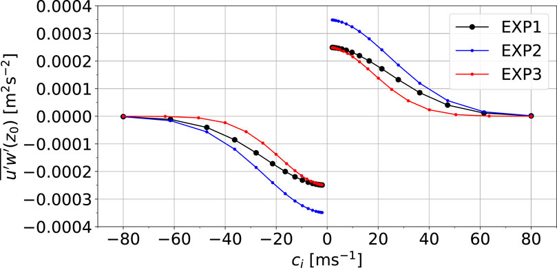
FIGURE 1. Spectra of GW momentum fluxes at the source level of the GW parameterization, $\overline{u^{\prime }{w}^{\prime }}\left(z_0\right)$, as a function of horizontal phase speeds $c_i$ for EXP1 (black), EXP2 (blue) and EXP3 (red).

3. Results

3.1. Background Circulation

We first study the results of the benchmark simulation (EXP1) based on the standard GW spectrum. Figure 2 shows altitude–latitude cross sections of the monthly mean zonal mean a) zonal (u) and b) meridional wind (v) as well as the c) neutral temperature (T) for Northern Hemisphere (NH) winter conditions (January). Figure 3 shows the GW effects in the same manner for a) zonal GW drag, b) meridional GW drag, and c) GW heating/cooling. A strong westerly wind system exceeding 80 m s⁻¹ is prevalent in the middle atmosphere in the NH, while summer easterlies dominate the Southern Hemisphere (SH). These middle atmosphere jets extend up to an altitude of about 90 km (Figure 2A) and significantly influence the upward propagation condition of small-scale GWs via wave filtering and critical level interactions. Thus, in the NH (winter) mainly westward directed GWs can propagate into the upper atmosphere, while the eastward directed GWs are substantially damped or largely filtered out. The opposite phenomenon prevails in the summer SH. This distribution of GW drag is clearly seen by the eastward GW drag in the SH and westward GW drag in the NH between 80 and 100 km (Figure 3A), which is primarily responsible for the reversal of the zonal mean flow above 90 km, from eastward to westward direction ($\sim -40$ m s⁻¹) in the winter NH and from westward to eastward direction in the SH ($\sim 50$ m s⁻¹). The GW drag with alternating sign above 100 km, for example, westward and eastward GW drag regime around 105–125 km in the SH and NH, respectively, is formed by the faster GW harmonics that have survived the filtering and nonlinear dissipation in the mesosphere (Yiğit et al., 2009). Owing to nonlinear interactions and increasing dissipation with altitude due to molecular diffusion and thermal conduction, the surviving faster GW harmonics are attenuated in the thermosphere and produce drag there. Overall, maximum GW drag is in the order of $\pm 100$ m s⁻¹ d⁻¹ and is stronger in the summer SH than the winter NH, which is in line with radar observations of GW fluxes and variance (Placke et al., 2011a; Placke et al., 2011b).

FIGURE 2

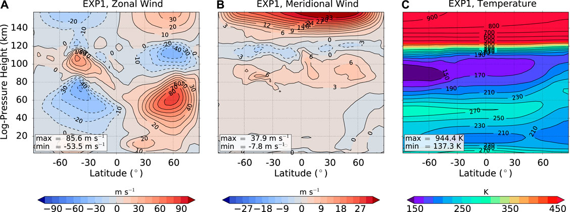
FIGURE 2. Zonal mean zonal wind (A), meridional wind (B), and temperature (C) for EXP1 simulation. Units in (A,B) m s⁻¹ and (C) K. Contour lines show intervals of (A) 10 m s⁻¹, (B) 3 m s⁻¹, and (C) 20 K (for $T<300$ K) and 100 K (for $T\ge 300$ K), respectively.

FIGURE 3

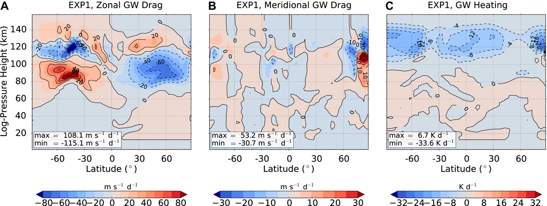
FIGURE 3. Same as Figure 2 but for zonal GW drag (A), meridional GW drag (B), and heating due to GWs (C). Units in (A,B) m s⁻¹ d⁻¹ and (C) K d⁻¹, respectively.

The mean meridional circulation (Figure 2B) is directed from the summer mesopause to the winter mesopause and has a maximum of 8 m s⁻¹ around 80 km. This is the upper branch of the so called Brewer–Dobsen Circulation. Like the zonal wind, the meridional winds also reverse the direction, e.g., winter to summer mean flow around 110 km. Overall, these circulation cells leading to the reversals in the zonal and meridional winds in the MLT are driven by GW dynamics. The associated changes in the residual mean circulation lead to the adiabatic cooling and warming of the summer and winter hemispheres, respectively, as can be seen by the temperature distribution in the MLT (Figure 2C). Owing to the strong northward winds at around 80 km, air descends and warms up the winter mesopause adiabatically ($\sim 180$ K), while it ascends and cools down adiabatically the summer mesopause ($<150$ K). During polar night, when the polar vortex establishes, there is a lack of incoming solar radiation so that the temperature is decreasing in the NH in the polar stratosphere. However, in the SH, the temperature rises up to 270 K in the polar stratosphere due to the absorption of solar radiation by ozone. Above 120 km in the thermosphere the temperature gradually increases, exceeding, e.g., 900 K in summer due primarily to the enhanced absorption of solar UV and EUV by molecular and atomic oxygen. GW heating and cooling [in K d⁻¹] presented in Figure 3C suggests that the thermal effects of GWs increase with increasing altitude in the thermosphere. The primary thermal effect of GWs is to cool the thermosphere above 120 km altitude, which is in agreement with previous studies (Yiğit and Medvedev, 2009; Yiǧit and Medvedev, 2017). The thermal effects of GWs are produced by the combination of the frictional heating and the differential (dynamic) cooling by dissipating GWs (Medvedev and Klaassen, 2003; Yiǧit et al., 2008).

We compare our results with reference climatologies such as the Upper Atmosphere Research Satellite (UARS) Reference Atmosphere Project (URAP; Swinbank and Ortland, 2003) or the Committee on Space Research (COSPAR) International Reference Atmosphere (CIRA-86; Fleming et al., 1988), with the more modern Global Empirical Wind Model (GEWM; Portnyagin et al., 2004; Jacobi et al., 2009) and the Horizontal Wind Model (HWM-14; Drob et al., 2015), and other GCMs like the extended Whole Atmosphere Community Climate Model (WACCM-X; Liu et al., 2018; Qian et al., 2019) and Kühlungsborn Mechanistic General Circulation Model (KMCM; Becker, 2017).

The overall mean structure of the middle atmosphere and lower thermosphere are well reproduced by the model except for i) the slightly overestimated mesospheric jet at 60 km between 50°N and 65°N, which reaches up to 80 m s⁻¹, and ii) the missing tilt of the mesospheric jet toward lower latitudes with increasing height. Samtleben et al. (2019) already reported a relatively large mesospheric jet in the MUAM model based on a tuned linear Lindzen-type GW parameterization, which was about 60 m⁻¹s⁻¹, being comparable to CIRA-86 and HWM-14, but about 20 m s⁻¹ larger than the jet maximum proposed by GEWM and URAP. Note, however, that GEWM is only available for altitudes between 70 and 100 km (slightly above our jet maximum) and URAP is interpolated for large areas near the jets. Due to the GW scheme according to Yiǧit et al. (2008), included in the present simulations, the mesospheric jet has strengthened by additional 20 m s⁻¹ and the jet maximum is slightly shifted toward the North compared to the MUAM simulations presented in the work by Samtleben et al. (2019). This poleward shift does not agree with URAP and other climatologies. The zonal wind jet is of similar magnitude as the one simulated by Miyoshi and Yiğit (2019), but again stronger than the one predicted by the WACCM-X model (Qian et al., 2019). As in WACCM-X, the magnitude and altitude–latitude structure of the meridional MLT wind jet in MUAM is comparable to the ones predicted by the radar-based GEWM (Portnyagin et al., 2004; Jacobi et al., 2009). Our results can also be compared with meteor radar retrievals of mesospheric winds in the $\sim 85$–90 km range. For example, in the zonal wind climatology determined by Pramitha et al. (2019) it is seen overall that weak eastward winds reverse direction to westward at higher altitudes during January at equatorial and low-latitudes in the NH, which is also seen in our simulations.

The easterly wind jet in the summer stratosphere is observed to be stronger (URAP: $-60$ to $-80$ m s⁻¹). Models like HWM-14 or GEWM produce weaker peaks near 50 to 60 m s⁻¹ but still larger than the MUAM results. However, in comparison to Samtleben et al. (2019), the new implementation of the GW scheme increased the jet speed by roughly 10 to 20 m s⁻¹ toward a more realistic value. In our simulations, we are missing the double-peak structure of the westerly jet and along with that more significant amplitudes to 80°S. As this was also the case in former MUAM versions (Lilienthal et al., 2017; Lilienthal and Jacobi, 2019; Samtleben et al., 2019), this is most likely not a weakness of the GW scheme but related to other model core dynamics. The wind reversal at about 90 km is realistic, compared to URAP, and the easterlies above reach 50 m s⁻¹, also comparable to URAP, HWM-14 or the CIRA climatology.

3.2. Effect of Modification of Gravity Wave Parameters

GW generation processes in the lower atmosphere are complex and a number of processes contribute to the formation of the GW spectrum. We next would like to test the response of the GCM to variations in the initial GW spectrum. Two more experiments have been performed as has been described in Section 2.1. The same mean fields are analyzed and presented for these simulations as has been done for EXP1. The field of a respective experiment is shown as contour lines, while the differences with respect to the benchmark run (i.e., EXP2-EXP1 and EXP3-EXP1) are given in color shading.

3.2.1. Modified GW Spectrum: Increased Flux at the Source Level

The impact of an increased GW flux at the source level on the mean circulation is shown in the difference plots in Figure 4. Figure 4A indicates that right below the region of eastward wind reversal in the SH and around the westward wind reversal in the NH, the mean zonal wind has become relatively westerly and easterly, respectively. Studying the associated GW drag results in Figure 5A can provide some insight into this result. Increasing the source maximum momentum strength affects primarily the dissipation altitude, thus the saturation level of individual GW harmonics as well as the associated drag produced by them. Larger momentum flux means that GWs dissipate at lower altitude due to increased nonlinear interactions in the MLT, which then enhances the mesospheric reversals in both hemispheres, as a consequence of the increased eastward and westward GW drag in the SH and NH around 80–100 km. The secondary enhancement of the westward GW drag takes place in the lower thermosphere, for example, in the SH around 120 km, owing to the enhanced dissipation of the surviving faster GW harmonics due to increasing molecular viscosity with height, which has been previously discussed.

FIGURE 4

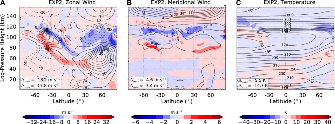
FIGURE 4. Contour lines: zonal mean (A) zonal wind, (B) meridional wind, and (C) temperature for EXP2 simulation in intervals of (A) 10 m s⁻¹, (B) 4 m s⁻¹, and (C) 20 K below 300 K and 100 K above. Color shading: differences EXP2-EXP1.

FIGURE 5

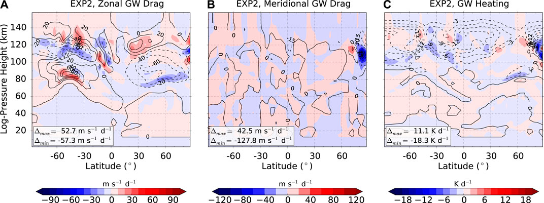
FIGURE 5. Same as Figure 4 but for (A) zonal GW drag, (B) meridional GW drag and (C) heating due to GWs in intervals of (A) 20 m s⁻¹ d⁻¹, (B) 15 m s⁻¹ d⁻¹ and (C) 3 K d⁻¹. Color shading: differences EXP2-EXP1.

The meridional circulation presented in Figure 4B shows a strengthening of the mesospheric circulation by 1–2 m s⁻¹, i.e., a stronger southward wind as well as an enhancement of the lower thermospheric mean northward circulation, which are primarily driven by the intensification of the mesospheric and lower thermospheric GW momentum deposition. Owing to the enhanced mesospheric meridional circulation the upward (downward) movement in the polar region in the SH (NH) intensifies, which leads to a stronger adiabatic cooling (warming). This effect can be seen in the mesospheric temperature differences (Figure 4C), which are negative (positive) in the SH (NH) around 80 km in the polar region with up to $-3$ K ($+5$ K). A similar effect but in the opposite sense happens in the lower thermosphere (around 110 km), where there is a relative adiabatic warming in the SH polar latitudes but a relative cooling in the NH middle to high latitudes. Higher up in the thermosphere ($>120$ km) the combined effect of the changes in the GW-induced mean meridional circulation and GW heating/cooling lead to a slight relative cooling of a few K d⁻¹ with respect to the control simulation, while the changes in the GW induced heating/cooling are overall relatively small (Figure 5C), despite the significant increase in the initial source strength. The only exception is the NH polarthermosphere below 100 km, where the GW heating/cooling characteristic dipole structure with respect to the altitude shows some intensification.

3.2.2. Modified Gravity Wave Spectrum: Same Total but Narrower Flux at the Source Level

We next present the simulation results of EXP3, in which we have increased the number of wave harmonics from 30 to 34, keeping the maximum phase speed, the total momentum flux, and the peak momentum flux the same as in the benchmark case, EXP1. For this purpose, the FWHM was reduced to $c_w=26$ m s⁻¹. This adjustment has shifted the phase speeds to slightly larger values in the tail of the spectrum, while significantly decreasing the individual momentum flux they carry (Figure 1). The impact of the spectral changes, primarily in the tail of the spectrum, which is now populated with slightly faster waves but with smaller wave fluxes can be seen in the zonal wind (Figure 6A). It shows that the height of the wind reversal is slightly shifted upward and its magnitude is reduced, indicated by the relative negative/positive zonal wind differences, EXP3-EXP1, around 100 km in the SH and NH, respectively. Overall, the strengths of the GW momentum flux controls the magnitude of the zonal wind reversal in the MLT. Higher up in the NH lower thermosphere, the easterlies become weaker by more than 20 m s⁻¹ compared to EXP1. These changes can be explained by the reduction of the momentum flux in the tail of the spectrum in EXP3 relative to EXP1.

FIGURE 6

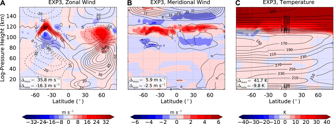
FIGURE 6. Contour lines: Zonal mean (A) zonal wind, (B) meridional wind and (C) temperature for EXP3 simulation in intervals of (A) 10 m s⁻¹, (B) 4 m s⁻¹, and (C) 20 K below 300 K and 100 K above. Color shading: differences EXP3-EXP1.

The meridional circulation (Figure 6B) in the mesosphere as well as in the thermosphere also shows a weakening. The southward wind (northward wind) between 80 and 100 km (100 and 120 km) is reduced by more than 2 m s⁻¹ (4 m s⁻¹). The weakening of both circulation patterns affects the intensity of the downward and upward movements in the polar region, which is therefore also less pronounced. This leads to a colder (warmer) winter (summer) mesopause, which can be seen in the negative (positive) temperature anomalies of $-3$ K ($+3$ K) shown in Figure 6C. In the polar thermosphere, the effect is even stronger with more than $+5$ K temperature difference. These changes are primarily controlled by the associated changes in the zonal GW drag, rather than by the changes in the meridional GW drag. The meridional GW drag anomalies are confined to the polar latitude in the NH MLT (Figure 7B). Up to 8–10 K d⁻¹ relative reduction in the resultant GW cooling controls the thermal budget of the lower thermosphere to a much lesser extent than the dynamical changes.

FIGURE 7

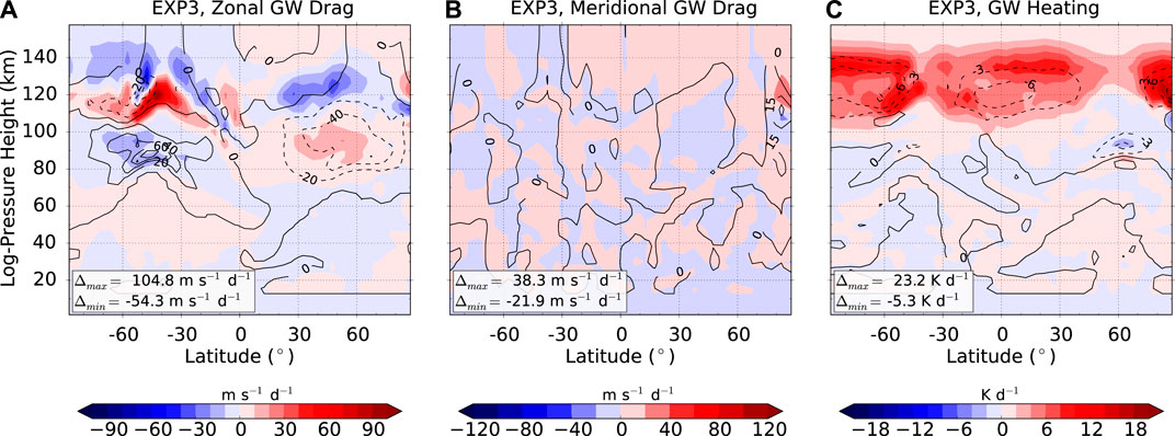
FIGURE 7. Same as Figure 6 but for (A) zonal GW drag, (B) meridional GW drag, and (C) heating due to GWs in intervals of (A) 20 m s⁻¹ d⁻¹, (B) 15 m s⁻¹ d⁻¹, and (C) 3 K d⁻¹.

Between 100 and 120 km the zonal GW drag difference (Figure 7A) shows a strong positive anomaly of more than $+50$ m s⁻¹ d⁻¹, which may be an effect of the vertical shift of the eastward directed zonal GW drag on the SH. While the zonal GW drag anomalies are stronger on the SH, the meridional GW drag anomalies (Figure 7B) are more pronounced in the NH, especially in the polar thermosphere. We observe a weakening of the meridional GW drag of more than 20 m s⁻¹ d⁻¹$$. Thereby, the region of southward directed GW drag near 120 km in EXP1 (Figure 3B) disappears in EXP3 (Figure 7B). The northward directed GW drag near 110 km, however, persists. With respect to the GW heating anomalies (Figure 7C), the induced cooling in the thermosphere is strongly reduced by more than 10 K d⁻¹. Thus, the EXP3 cooling is half the EXP1 cooling.

Note that in EXP2, we had increased the source peak momentum flux by more than a factor of 1.5. This corresponds to increasing the momentum flux of each GW harmonic by $50\text{\%}$ as well as the total momentum flux by $50\text{\%}$. In EXP3, however, we have kept the total momentum flux constant, as well as the peak momentum flux and the phase speed range, varying only the FWHM of the spectrum and the number of harmonics. Interestingly, the response of the mesosphere and lower thermosphere in terms of changes in circulation patterns and temperature distributions are stronger in EXP3 than in EXP2, which emphasizes the dynamical significance of the faster (nonorographic) GWs for the structure of the mesosphere and lower thermosphere. This means that uncertainty in the peak momentum flux of the GW spectrum has less impact than the uncertainty in the spectral shape of the spectrum on the structure of the atmosphere up to the lower thermosphere.

3.3. Relation Between Gravity Waves and Terdiurnal Tides

The migrating TDT amplitudes and phases in the zonal wind, meridional wind, and temperature are shown in Figure 8 for the benchmark simulation EXP1. The amplitudes of all components have a maximum in the lower thermosphere between 120 and 140 km, being larger in the summer SH than winter NH. Ground based radar observations and satellite measurements of the TDT activity have overall focused on the MLT region between 80 and 110 km and have reported an autumn and winter maximum of the TDT amplitudes (e.g., Beldon et al., 2006; Jacobi, 2012; Liu et al., 2019; Pancheva et al., 2013; Yue et al., 2013). The TDT amplitudes simulated by the GCM are also larger in the winter hemisphere than the summer hemisphere in the MLT, in relatively good agreement with these measurements. Vertical wavelengths in the MLT and above, taken from the vertical TDT phase gradients in Figures 8D–F, are on the order of 30 km in the summer hemisphere, but larger in winter. This agrees with radar observations (Bernard et al., 1981; Thayaparan, 1997; Namboothiri et al., 2004; Zhao et al., 2005; Jacobi, 2012). In summer, wavelengths between 30 km (Jacobi, 2012) and more than 100 km (Thayaparan, 1997; Namboothiri et al., 2004) have been observed which is longer than a typical DT and rather comparable to vertical wavelengths of the SDT. In winter, the vertical phase gradient is often close to zero and thus wavelengths of more than 1,000 km are possible (Thayaparan, 1997; Namboothiri et al., 2004; Zhao et al., 2005; Jacobi, 2012).

FIGURE 8

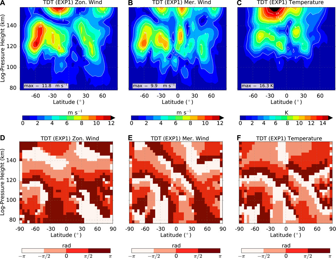
FIGURE 8. Zonal mean TDT amplitudes of (A) zonal wind (in m s⁻¹), (B) meridional wind (in m s⁻¹) and (C) temperature (in K) for EXP1. (D–F) Corresponding TDT phases (in radians).

The most important dynamical feature in the lower thermosphere in our modeling study are GWs of lower atmospheric origin parameterized by the whole atmosphere nonlinear GW parameterization, and therefore they are the most obvious candidate for tidal modulation at those heights. We next want to examine their influence on the TDT. The terdiurnal components of the GW parameters presented in Figure 9 can be used as a proxy for GW–TDT interactions. The amplitudes of terdiurnal GW drag and heating maximize near 120–130 km, where TDT amplitudes in temperature and wind maximize as well. This indicates that the TDT in the thermosphere is strongly influenced by the momentum deposition of dissipating GWs. To give an example, the zonal wind TDT at southern midlatitudes reaches about 10 m s⁻¹ (see Figure 8A), while the terdiurnal zonal GW drag there is about 6 m s⁻¹ d⁻¹ (Figure 9A). In other words, our simulation suggests that GWs have the potential to change the tidal amplitudes within 6 h by about $\mathrm{1,5}$ m s⁻¹, or $15\text{\%}$. We also present phases of terdiurnal GW drag and heating in Figures 9D–F. Similar to the wind and temperature TDT (Figures 8D–F), the phases of the terdiurnal GW effects are rather irregular in the mesosphere but become more organized in the lower thermosphere with longer vertical wavelengths.

FIGURE 9

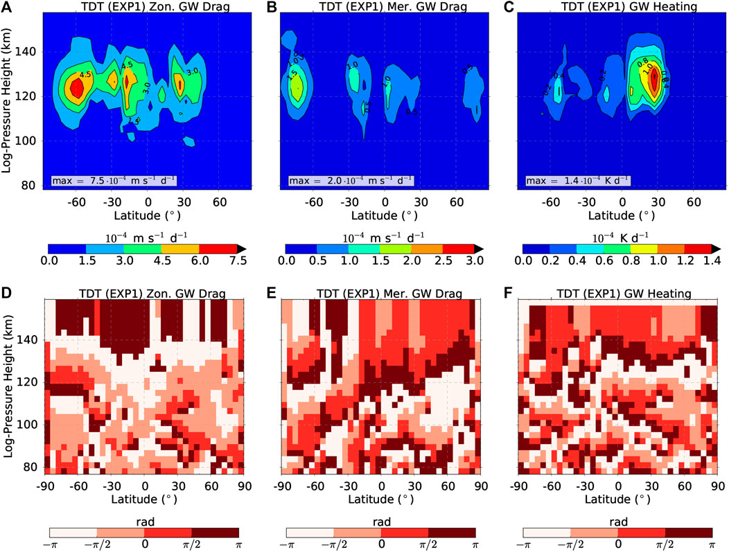
FIGURE 9. Same as Figure 8 but for TDT amplitudes of (A) zonal GW drag (in m s⁻¹ d⁻¹), (B) meridional GW drag (in m s⁻¹ d⁻¹), (C) heating due to GWs (in K d⁻¹), and (D–F) corresponding phases (in radians).

Figures 10A–C show the TDT amplitudes for the simulation EXP2 (contour lines), i.e. the one with increased GW source flux, and their differences with respect to EXP1 (color shading). Their general structure in wind and temperature is similar to that of EXP1 (Figures 8A–C). Differences EXP2-EXP1 amount to $\pm 1$ to $\pm 2$ m s⁻¹ and K. The terdiurnal signature in GW parameters (Figures 10D–F) are mainly increased near their maxima, which can be interpreted as a direct result of the increased source momentum flux in simulation EXP2. There are also some negative changes between EXP2 and EXP1, but these are rather irregular and most likely a result of the slightly altered background climatology described in Section 3.2, influencing wave propagation conditions in general.

FIGURE 10

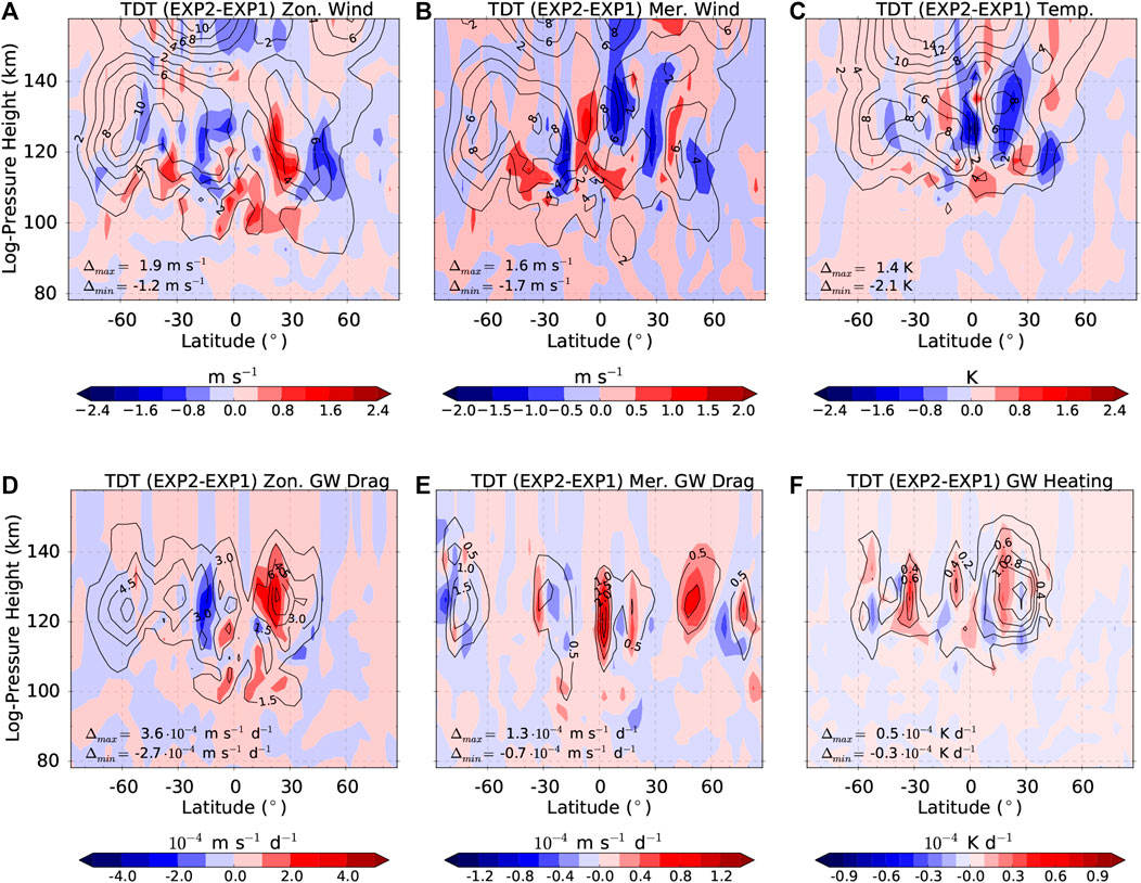
FIGURE 10. Zonal mean TDT amplitudes of EXP2 for (A) zonal wind, (B) meridional wind, (C) temperature, (D) zonal GW drag, (E) meridional GW drag and (F) heating due to GWs (black contour lines). Intervals are (A,B) 2 m s⁻¹, (C) 2 K, (D)$1.5\cdot {10}^{-4}$ m s⁻¹ d⁻¹, (E)$0.5\cdot {10}^{-4}$ m s⁻¹ d⁻¹, and (F)$0.2\cdot {10}^{-4}$ K d⁻¹. Positive/negative differences EXP2-EXP1 ($\text{Δ}$) are shaded in red/blue. Their maximum/minimum values (${\text{Δ}}_{max}$/${\text{Δ}}_{min}$) are given in each panel.

Furthermore, there is good agreement between the TDT amplitude changes in the zonal wind (Figure 10A) and zonal GW drag (Figure 10D). For example, the latter one is increased at northern low latitudes at about 120–140 km and decreased at southern low latitudes at a similar altitude. This pattern is visible in TDT zonal wind amplitude changes, as well. In the meridional components (Figure 10B), the positive/negative change patterns also largely agree. In the thermal component (Figure 10C), however, the TDT temperature amplitude seems to be damped where the difference in terdiurnal GW heating is positive.

Figure 11 is similar to Figure 10, but refers to the differences between EXP3 and EXP1. This means that differences are based on a GW spectrum with more harmonics in EXP3 than in EXP1, but a smaller momentum flux for each individual harmonic, in particular in the mid-range phase speeds (see Figure 1). As a result, the sign in the EXP3-EXP1 differences of terdiurnal GW parameters is opposite to that of EXP2-EXP1 differences, i.e., it is negative almost everywhere (see Figures 11D–F). Accordingly, the TDT wind amplitudes (Figures 11A and 11B) are also mostly smaller in the EXP3 simulation compared to EXP1, decreasing by about 1–2 m s⁻¹ in the area of maximum amplitudes. They partly increase by a similar magnitude, but the decrease dominates, especially in the zonal wind component. Similar to the differences of EXP2-EXP1, the relation between terdiurnal GW heating (Figure 11F) and TDT temperature amplitude (Figure 11C) is less clear and we also observe large patches of positive amplitude changes up to 1.5 K in the temperature component that seem to be corresponding to negative GW heating.

FIGURE 11

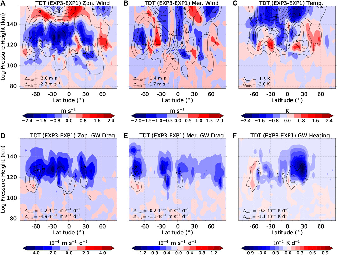
FIGURE 11. Same as Figure 10 but for EXP3 (contour lines) and differences EXP3-EXP1 (color shading).

4. Discussion and Conclusion

We have successfully implemented the whole-atmosphere (tropopause to thermosphere) nonlinear GW parameterization according to Yiǧit et al. (2008) into the mechanistic MUAM GCM. This benchmark simulation is labeled EXP1. The zonal mean horizontal wind patterns in the middle atmosphere as well as the global temperature distribution reasonably agree with respect to established climatologies such as CIRA-86 (Fleming et al., 1988) or URAP (Swinbank and Ortland, 2003), GEWM (Portnyagin et al., 2004; Jacobi et al., 2009), HWM-14 (Drob et al., 2015), and other GCM predictions like WACCM-X (Liu et al., 2018) or KMCM (Becker, 2017). The typical tilt of the zonal mesospheric jet toward lower latitudes with increasing height (e.g., Swinbank and Ortland, 2003; Drob et al., 2015; Becker, 2017) is missing here however. Instead, the jet is shifted poleward which is not realistical. Furthermore, wind speeds of the jet are relatively large. This could be due to a combination of issues associated with the GW source spectrum, lower boundary conditions, and model dynamical core. It cannot be directly attributed to the new GW scheme implementation as other models using the same scheme show different results (e.g., Miyoshi and Yiğit, 2019). Nevertheless, we have successfully simulated the self-consistent direct GW penetration into the thermosphere as has been previously done by other GCMs using the whole atmosphere scheme (Yiǧit et al., 2009; Miyoshi and Yiğit, 2019). Compared to earlier MUAM versions that use a highly tuned linear Lindzen-type GW parameterization for the middle atmosphere (e.g., Jacobi et al., 2015; Lilienthal and Jacobi, 2019; Samtleben et al., 2019), the winter mesospheric jet is enhanced in the present simulations. Therefore, it is also larger compared to other GCMs like WACCM-X or KMCM by about 20–40 m s⁻¹, depending on the respective model. Compared to the earlier Lindzen-type scheme, the nonlinear wave—wave interactions in our scheme lead to breaking levels lower in the atmosphere with smaller GW drag, which is more realistic (Medvedev et al., 1998). No artificial tuning factors have been used in our scheme and GW momentum deposition occurs naturally over a range of altitudes. In the lower thermosphere, the main impact of the whole atmosphere GW parameterization is to drive a vertical/meridional circulation, mainly by the GWs with high phase speeds, which are able to propagate through the MLT wind jets. Concerning the structure of the terdiurnal tide, typical autumn and winter maxima at midlatitudes, as reported by radar and satellite measurements (e.g., Beldon et al., 2006; Jacobi, 2012; Pancheva et al., 2013; Yue et al., 2013; Liu et al., 2019) are well reproduced by MUAM. As described above, vertical wavelengths agree with radar observations (Bernard et al., 1981; Thayaparan, 1997; Namboothiri et al., 2004; Zhao et al., 2005; Jacobi, 2012).

We performed two further experiments to investigate the response of the middle and upper atmosphere climatology to changes of the initial GW spectrum and horizontal momentum flux. In the experiment EXP2, we increased the momentum flux at the source level by roughly $50\text{\%}$ of the original value, while keeping the spectral shape unchanged. As expected, these modifications result in a stronger GW dissipation at lower levels (near 80 km), connected with a slightly intensified wind reversal in the MLT. This intensifies both the upper mesosphere and lower thermosphere meridional winds, related to stronger adiabatic warming/cooling of the winter mesosphere/lower thermosphere and reverse effects in the summer hemisphere. However, it turns out that the relatively drastic change of the peak source momentum flux does not influence the global dynamical patterns by such a large degree. One may conclude that an adjustment of this parameter is not crucial for the implementation of this GW parameterization into a GCM like MUAM.

In the final experiment (EXP3), the total momentum flux was kept constant with respect to the benchmark case EXP1, but the total number of harmonics was increased and the width of the spectrum was decreased, yielding smaller fluxes for the high phase speed tail of the spectrum. In this experiment, the mesospheric wind system was less affected, but the lower thermospheric jets were weakened, connected with cooling/warming of the winter/summer mesosphere, and reversed thermal effects above. Considering EXP2 and EXP3 with respect to the benchmark case, in general, the lower thermospheric circulation and temperature distributions responded more strongly to the changes in the spectral shape of the GW spectrum to the increase in the peak momentum flux. This emphasizes the dynamical significance of the faster GWs for the structure of the lower thermosphere, as these waves are less affected by dissipation and filtering processes in the stratosphere and mesosphere, and thus penetrate into the thermosphere (e.g., Hocke and Schlegel, 1996; Fritts and Alexander, 2003; Yiǧit et al., 2008, Yiǧit et al., 2009; Yiǧit and Medvedev, 2017).

For the first time, we investigated the effect of the GW source distribution on the amplitudes of the TDT using a nonlinear GW parameterization that extends up to the thermosphere. This gives us a more confident basis to study the GW—TDT interactions as the new GW scheme in MUAM, compared to the earlier coupled parameterizations, can much better describe the propagation of subgrid-scale GWs through the mesosphere into the thermosphere. The simulated latitudinal-vertical distribution of TDT amplitudes, and their vertical wave structure was found to be realistic when compared with observations. Modifications of the GW source spectrum or total momentum flux mainly influence the TDT in the lower thermosphere, and to a much lesser degree in the upper mesosphere. We found that increasing the GW momentum flux essentially leads to an increased terdiurnal variation in the GW drag and increased amplitudes in the lower thermosphere, which we interpret as a direct result of increased momentum flux of fast GWs. In turn, narrowing of the width of the GW spectrum mostly leads to a reduced terdiurnal variation in the GW drag and lower TDT amplitudes, as a consequence of the reduced momentum flux of fast GWs in the lower thermosphere. Miyahara and Forbes (1991) already demonstrated in their simulations that an interaction between the DT and GWs can generate a secondary TDT. Recently, GW—tide interactions were again underlined as an important excitation mechanism of the TDT (Lilienthal et al., 2018; Lilienthal and Jacobi, 2019). As a consequence of GW dynamical effects on the large-scale circulation, it is reasonable that a modified GW drag also strongly influences the TDT amplitudes as has been shown in our simulations.

Our modeling experiments highlight the importance of taking into account self-consistent propagation of GWs and their dissipation in the mesosphere and lower thermosphere. We could show the robustness of the nonlinear parameterization used here with respect to different GW phase speed spectra. The sensitivity tests are all within the range of uncertainties of the observed GW parameters in the lower atmosphere. In the MLT region, GWs play a crucial role for circulation patterns and temperature variations as well as for the TDTs. It is noteworthy that small modifications of momentum fluxes of fast GWs have substantial impact on the lower thermosphere mean circulation, and also on tidal amplitudes in particular with respect to the TDT.

Data Availability Statement

The datasets presented in this study can be found in online repositories. The names of the repository/repositories and accession number(s) can be found below: https://zenodo.org/record/3628282#.XyIQbBNKh-U.

Author Contributions

FL designed and performed the MUAM model runs together with NS. The first version was drafted by EY (introduction), FL and NS (main part) and CJ (summary). In later versions, EY contributed significantly toward finalizing the main part. All authors discussed the results.

Funding

FL, NS, and CJ acknowledge support by DFG through grants JA836/30-1, JA836/32-1, and JA836/38-1.

Conflict of Interest

The authors declare that the research was conducted in the absence of any commercial or financial relationships that could be construed as a potential conflict of interest.

References

Baumgarten, K., Gerding, M., Baumgarten, G., and Lübken, F.-J. (2018). Temporal variability of tidal and gravity waves during a record long 10-day continuous lidar sounding. Atmos. Chem. Phys. 18, 371–384. doi:10.5194/acp-18-371-2018

CrossRef Full Text | Google Scholar

Becker, E. (2017). Mean-flow effects of thermal tides in the mesosphere and lower thermosphere. J. Atmos. Sci. 74, 2043–2063. doi:10.1175/JAS-D-16-0194.1

CrossRef Full Text | Google Scholar

Becker, E., and Vadas, S. L. (2020). Explicit global simulation of gravity waves in the thermosphere. J. Geophys. Res. Space Phys. 125, e2020JA028034. doi:10.1029/2020JA028034

CrossRef Full Text | Google Scholar

Beldon, C. L., Muller, H. G., and Mitchell, N. J. (2006). The 8-hour tide in the mesosphere and lower thermosphere over the UK, 1988-2004. J. Atmos. Sol. Terr. Phys. 68, 655–668. doi:10.1016/j.jastp.2005.10.004

CrossRef Full Text | Google Scholar

Beres, J. H., Alexander, M. J., and Holton, J. R. (2004). A method of specifying the gravity wave spectrum above convection based on latent heating properties and background wind. J. Atmos. Sci. 61, 324–337. doi:10.1175/1520-0469(2004)061<0324:amostg>2.0.co;2

CrossRef Full Text | Google Scholar

Bernard, R., Fellous, J. L., Massebeuf, M., and Glass, M. (1981). Simultaneous meteor radar observations at Monpazier (France, 44°N) and Punta Borinquen (Puerto-Rico, 18°N). I-latitudinal variations of atmospheric tides. J. Atmos. Terr. Phys. 43, 525–533. doi:10.1016/0021-9169(81)90114-8

CrossRef Full Text | Google Scholar

Creasey, J. E., Forbes, J. M., and Hinson, D. P. (2006a). Global and seasonal distribution of gravity wave activity in Mars' lower atmosphere derived from MGS radio occultation data. Geophys. Res. Lett. 33, L01803. doi:10.1029/2005GL024037

CrossRef Full Text | Google Scholar

Creasey, J. E., Forbes, J. M., and Keating, G. M. (2006b). Density variability at scales typical of gravity waves observed in Mars’ thermosphere by the MGS accelerometer. Geophys. Res. Lett. 33, L22814. doi:10.1029/2006GL027583

CrossRef Full Text | Google Scholar

de la Torre, A., Alexander, P., Llamedo, P., Hierro, R., Nava, B., Radicella, S., et al. (2014). Wave activity at ionospheric heights above the Andes mountains detected from FORMOSAT-3/COSMIC GPS radio occultation data. J. Geophys. Res. Space Phys. 119, 2046–2051. doi:10.1002/2013JA018870

CrossRef Full Text | Google Scholar

Dee, D. P., Uppala, S. M., Simmons, A. J., Berrisford, P., Poli, P., Kobayashi, S., et al. (2011). The ERA-interim reanalysis: configuration and performance of the data assimilation system. Q. J. R. Meteorol. Soc. 137, 553–597. doi:10.1002/qj.828

CrossRef Full Text | Google Scholar

Drob, D. P., Emmert, J. T., Meriwether, J. W., Makela, J. J., Doornbos, E., Conde, M., et al. (2015). An update to the horizontal wind model (HWM): the quiet time thermosphere. Earth Space Sci. 2, 301–319. doi:10.1002/2014EA000089

CrossRef Full Text | Google Scholar

Fleming, E. L., Chandra, S., Barnett, J. J., and Corney, M. (1988). Zonal mean temperature, pressure, zonal wind and geopotential height as functions of latitude. Adv. Space Res. 10, 11–59. doi:10.1016/02731177(90)90386-E

Google Scholar

Fomichev, V. I., and Shved, G. M. (1985). Parameterization of the radiative flux divergence in the 9.6 μm O3 band. J. Atmos. Terr. Phys. 47, 1037–1049. doi:10.1016/0021-9169(85)90021-2

CrossRef Full Text | Google Scholar

Forbes, J. M., Bruinsma, S. L., Doornbos, E., and Zhang, X. (2016). Gravity wave-induced variability of the middle thermosphere. J. Geophys. Res. Space Phys. 121, 6914–6923. doi:10.1002/2016JA022923

CrossRef Full Text | Google Scholar

Forbes, J. M., Jun, G., and Saburo, M. (1991). On the interactions between gravity waves and the diurnal propagating tide. Planet. Space Sci. 39, 1249–1257. doi:10.1016/0032-0633(91)90038-C

CrossRef Full Text | Google Scholar

Fritts, D. C., and Alexander, M. J. (2003). Gravity wave dynamics and effects in the middle atmosphere. Rev. Geophys. 41, 1003. doi:10.1029/2001RG000106

CrossRef Full Text | Google Scholar

Fritts, D. C., and Lund, T. S. (2011). “Gravity wave influences in the thermosphere and ionosphere: observations and recent modeling,” in Aeronomy of the earth’s atmosphere and ionosphere. Editors M. Abdu, and D. Pancheva (Dordrecht, Netherlands: Springer Netherlands), Vol. 2, 109–130.

Google Scholar

Gavrilov, N. M., and Kshevetskii, S. P. (2015). Dynamical and thermal effects of nonsteady nonlinear acoustic-gravity waves propagating from tropospheric sources to the upper atmosphere. Adv. Space Res. 56, 1833–1843. doi:10.1016/j.asr.2015.01.033

CrossRef Full Text | Google Scholar

Heale, C. J., Bossert, K., Vadas, S. L., Hoffmann, L., Dörnbrack, A., Stober, G., et al. (2020). Secondary gravity waves generated by breaking mountain waves over Europe. J. Geophys. Res. Atmos. 125, e2019JD031662. doi:10.1029/2019JD031662

CrossRef Full Text | Google Scholar

Heale, C. J., Snively, J. B., Hickey, M. P., and Ali, C. J. (2014). Thermospheric dissipation of upward propagating gravity wave packets. J. Geophys. Res. Space Phys. 119, 3857–3872. doi:10.1002/2013JA019387

CrossRef Full Text | Google Scholar

Hickey, M. P., Schubert, G., and Walterscheid, R. L. (2009). Propagation of tsunami-driven gravity waves into the thermosphere and ionosphere. J. Geophys. Res. 114, A08304. doi:10.1029/2009JA014105

CrossRef Full Text | Google Scholar

Hines, C. O. (1960). Internal atmospheric gravity waves at ionospheric heights. Can. J. Phys. 38, 1441–1481. doi:10.1139/p60-150

CrossRef Full Text | Google Scholar

Hocke, K., and Schlegel, K. (1996). A review of atmospheric gravity waves and travelling ionospheric disturbances: 1982-1995. Ann. Geophys. 14, 917–940. doi:10.1007/s00585-996-0917-6

CrossRef Full Text | Google Scholar

Holton, J. R. (1982). The role of gravity wave induced drag and diffusion in the momentum budget of the mesosphere. J. Atmos. Sci. 39, 791–799. doi:10.1175/1520-0469(1982)039<0791:trogwi>2.0.co;2

CrossRef Full Text | Google Scholar

Jacobi, C. (2012). 6 year mean prevailing winds and tides measured by VHF meteor radar over Collm (51.3°N, 13.0°E). J. Atmos. Sol. Terr. Phys. 78–79, 8–18. doi:10.1016/j.jastp.2011.04.010

CrossRef Full Text | Google Scholar

Jacobi, C., Fröhlich, K., and Pogoreltsev, A. (2006). Quasi two-day-wave modulation of gravity wave flux and consequences for the planetary wave propagation in a simple circulation model. J. Atmos. Sol. Terr. Phys. 68, 283–292. doi:10.1016/j.jastp.2005.01.017

CrossRef Full Text | Google Scholar

Jacobi, C., Fröhlich, K., Portnyagin, Y., Merzlyakov, E., Solovjova, T., Makarov, N., et al. (2009). Semi-empirical model of middle atmosphere wind from the ground to the lower thermosphere. Adv. Space Res. 43, 239–246. doi:10.1016/j.asr.2008.05.011

CrossRef Full Text | Google Scholar

Jacobi, C., Lilienthal, F., Geißler, C., and Krug, A. (2015). Long-term variability of mid-latitude mesosphere-lower thermosphere winds over Collm (51°N, 13°E). J. Atmos. Sol. Terr. Phys. 136, 174–186. doi:10.1016/j.jastp.2015.05.006

CrossRef Full Text | Google Scholar

Jakobs, H. J., Bischof, M., Ebel, A., and Speth, P. (1986). Simulation of gravity wave effects under solstice conditions using a 3-d circulation model of the middle atmosphere. J. Atmos. Terr. Phys. 48, 1203–1223. doi:10.1016/0021-9169(86)90040-1

CrossRef Full Text | Google Scholar

Kim, Y., Eckermann, S. D., and Chun, H. (2003). An overview of the past, present and future of gravity-wave drag parametrization for numerical climate and weather prediction models. Atmos. Ocean. 41, 65–98. doi:10.3137/ao.410105

Google Scholar

Lilienthal, F., Jacobi, C., and Geißler, C. (2018). Forcing mechanisms of the terdiurnal tide. Atmos. Chem. Phys. 18, 15725–15742. doi:10.5194/acp-18-15725-2018

CrossRef Full Text | Google Scholar

Lilienthal, F., and Jacobi, C. (2019). Nonlinear forcing mechanisms of the migrating terdiurnal solar tide and their impact on the zonal mean circulation. Ann. Geophys. 37, 943–953. doi:10.5194/angeo-37-943-2019

CrossRef Full Text | Google Scholar

Lilienthal, F., Jacobi, C., Schmidt, T., de la Torre, A., and Alexander, P. (2017). On the influence of zonal gravity wave distributions on the southern hemisphere winter circulation. Ann. Geophys. 35, 785–798. doi:10.5194/angeo-35-785-2017

CrossRef Full Text | Google Scholar

Lindzen, R. S. (1981). Turbulence and stress owing to gravity wave and tidal breakdown. J. Geophys. Res. 86, 9707–9714. doi:10.1029/JC086iC10p09707

CrossRef Full Text | Google Scholar

Liu, H.-L., McInerney, J. M., Santos, S., Lauritzen, P. H., Taylor, M. A., and Pedatella, N. M. (2014). Gravity waves simulated by high-resolution whole atmosphere community climate model. Geophys. Res. Lett. 41, 9106–9112. doi:10.1002/2014GL062468

CrossRef Full Text | Google Scholar

Liu, H. L., Bardeen, C. G., Foster, B. T., Lauritzen, P., Liu, J., Lu, G., et al. (2018). Development and validation of the whole atmosphere community climate model with thermosphere and ionosphere extension (WACCM‐X 2.0). J. Adv. Model. Earth Syst. 10, 381–402. doi:10.1002/2017MS001232

CrossRef Full Text | Google Scholar

Liu, H., Tsutsumi, M., and Liu, H. (2019). Vertical structure of terdiurnal tides in the Antarctic MLT region: 15‐year observation over Syowa (69°S, 39°E). Geophys. Res. Lett. 46, 2364–2371. doi:10.1029/2019GL082155

CrossRef Full Text | Google Scholar

Manson, A. H., Meek, C. E., Koshyk, J., Franke, S., Fritts, D. C., Riggin, D., et al. (2002). Gravity wave activity and dynamical effects in the middle atmosphere (60-90 km): observations from an MF/MLT radar network, and results from the Canadian middle atmosphere model (CMAM). J. Atmos. Sol. Terr. Phys. 64, 65–90. doi:10.1016/s1364-6826(01)00097-9

CrossRef Full Text | Google Scholar

McFarlane, N. A. (1987). The effect of orographically excited gravity wave drag on the general circulation of the lower stratosphere and troposphere. J. Atmos. Sci. 44, 1775–1800. doi:10.1175/1520-0469(1987)044<1775:teooeg>2.0.co;2

CrossRef Full Text | Google Scholar

Medvedev, A. S., Klaassen, G. P., and Beagley, S. R. (1998). On the role of an anisotropic gravity wave spectrum in maintaining the circulation of the middle atmosphere. Geophys. Res. Lett. 25, 509–512. doi:10.1029/98GL50177

CrossRef Full Text | Google Scholar

Medvedev, A. S., and Klaassen, G. P. (2000). Parameterization of gravity wave momentum deposition based on nonlinear wave interactions: basic formulation and sensitivity tests. J. Atmos. Sol. Terr. Phys. 62, 1015–1033. doi:10.1016/s1364-6826(00)00067-5

CrossRef Full Text | Google Scholar

Medvedev, A. S., and Klaassen, G. P. (2003). Thermal effects of saturating gravity waves in the atmosphere. J. Geophys. Res. 108, 4040. doi:10.1029/2002JD002504

CrossRef Full Text | Google Scholar

Medvedev, A. S., and Yiğit, E. (2019). Gravity waves in planetary atmospheres: their effects and parameterization in global circulation models. Atmosphere 10, 531. doi:10.3390/atmos10090531

CrossRef Full Text | Google Scholar

Medvedev, A. S., Yiğit, E., Hartogh, P., and Becker, E. (2011). Influence of gravity waves on the Martian atmosphere: general circulation modeling. J. Geophys. Res. 116, E10004. doi:10.1029/2011JE003848

CrossRef Full Text | Google Scholar

Medvedev, A. S., Yiğit, E., and Hartogh, P. (2017). Ion friction and quantification of the geomagnetic influence on gravity wave propagation and dissipation in the thermosphere-ionosphere. J. Geophys. Res. Space Phys. 122, 12464–12475. doi:10.1002/2017JA024785

CrossRef Full Text | Google Scholar

Miyahara, S., and Forbes, J. M. (1991). Interactions between gravity waves and the diurnal tide in the mesosphere and lower thermosphere. J. Meteorol. Soc. Jpn. 69, 523–531. doi:10.2151/jmsj1965.69.5_523

CrossRef Full Text | Google Scholar

Miyoshi, Y., Forbes, J. M., and Moudden, Y. (2011). A new perspective on gravity waves in the Martian atmosphere: sources and features. J. Geophys. Res. 116, E09009. doi:10.1029/2011JE003800

CrossRef Full Text | Google Scholar

Miyoshi, Y., Fujiwara, H., Jin, H., and Shinagawa, H. (2014). A global view of gravity waves in the thermosphere simulated by a general circulation model. J. Geophys. Res. Space Phys. 119, 5807–5820. doi:10.1002/2014JA019848

CrossRef Full Text | Google Scholar

Miyoshi, Y., and Yiğit, E. (2019). Impact of gravity wave drag on the thermospheric circulation: implementation of a nonlinear gravity wave parameterization in a whole-atmosphere model. Ann. Geophys. 37, 955–969. doi:10.5194/angeo-37-955-2019

CrossRef Full Text | Google Scholar

Namboothiri, S. P., Kishore, P., Murayama, Y., and Igarashi, K. (2004). MF radar observations of terdiurnal tide in the mesosphere and lower thermosphere at Wakkanai, Japan. J. Atmos. Sol. Terr. Phys. 66, 241–250. doi:10.1016/j.jastp.2003.09.010

CrossRef Full Text | Google Scholar

Nayak, C., and Yiğit, E. (2019). Variation of small‐scale gravity wave activity in the ionosphere during the major sudden stratospheric warming event of 2009. J. Geophys. Res. Space Phys. 124, 470–488. doi:10.1029/2018JA026048

CrossRef Full Text | Google Scholar

Nicolls, M. J., and Heinselman, C. J. (2007). Three-dimensional measurements of traveling ionospheric disturbances with the poker flat incoherent scatter radar. Geophys. Res. Lett. 34, L21104. doi:10.1029/2007GL031506

CrossRef Full Text | Google Scholar

Nicolls, M. J., Vadas, S. L., Aponte, N., and Sulzer, M. P. (2014). Horizontal parameters of daytime thermospheric gravity waves andEregion neutral winds over Puerto Rico. J. Geophys. Res. Space Phys. 119, 575–600. doi:10.1002/2013JA018988

CrossRef Full Text | Google Scholar

Pancheva, D., Mukhtarov, P., and Smith, A. K. (2013). Climatology of the migrating terdiurnal tide (TW3) in SABER/TIMED temperatures. J. Geophys. Res. Space Phys. 118, 1755–1767. doi:10.1002/jgra.50207

CrossRef Full Text | Google Scholar

Parish, H. F., Schubert, G., Hickey, M. P., and Walterscheid, R. L. (2009). Propagation of tropospheric gravity waves into the upper atmosphere of Mars. Icarus 203, 28–37. doi:10.1016/j.icarus.2009.04.031

CrossRef Full Text | Google Scholar

Park, J., Lühr, H., Lee, C., Kim, Y. H., Jee, G., and Kim, J.-H. (2014). A climatology of medium-scale gravity wave activity in the midlatitude/low-latitude daytime upper thermosphere as observed by CHAMP. J. Geophys. Res. Space Phys. 119, 2187–2196. doi:10.1002/2013JA019705

CrossRef Full Text | Google Scholar

Placke, M., Hoffmann, P., Becker, E., Jacobi, C., Singer, W., and Rapp, M. (2011a). Gravity wave momentum fluxes in the MLT-Part II: meteor radar investigations at high and midlatitudes in comparison with modeling studies. J. Atmos. Sol. Terr. Phys. 73, 911–920. doi:10.1016/j.jastp.2010.05.007

CrossRef Full Text | Google Scholar

Placke, M., Stober, G., and Jacobi, C. (2011b). Gravity wave momentum fluxes in the MLT-Part I: seasonal variation at Collm (51.3°N, 13.0°E). J. Atmos. Sol. Terr. Phys. 73, 904–910. doi:10.1016/j.jastp.2010.07.012

CrossRef Full Text | Google Scholar

Pogoreltsev, A. I. (2007). Generation of normal atmospheric modes by stratospheric vacillations. Izvestiya Atmos. Ocean. Phys. 43, 423–435. doi:10.1134/S0001433807040044

Google Scholar

Pogoreltsev, A. I., Vlasov, A. A., Fröhlich, K., and Jacobi, C. (2007). Planetary waves in coupling the lower and upper atmosphere. J. Atmos. Sol. Terr. Phys. 69, 2083–2101. doi:10.1016/j.jastp.2007.05.014 CrossRef Full Text

CrossRef Full Text | Google Scholar

Portnyagin, Y., Solovjova, T., Merzlyakov, E., Forbes, J., Palo, S., Ortland, D., et al. (2004). Mesosphere/lower thermosphere prevailing wind model. Adv. Space Res. 34, 1755–1762. doi:10.1016/j.asr.2003.04.058

CrossRef Full Text | Google Scholar

Pramitha, M., Kishore Kumar, K., Venkat Ratnam, M., Rao, S. V. B., and Ramkumar, G. (2019). Meteor radar estimations of gravity wave momentum fluxes: evaluation using simulations and observations over three tropical locations. J. Geophys. Res. Space Phys. 124, 7184–7201. doi:10.1029/2019JA026510

CrossRef Full Text | Google Scholar

Qian, L., Jacobi, C., and McInerney, J. (2019). Trends and solar irradiance effects in the mesosphere. J. Geophys. Res. Space Phys. 124, 1343–1360. doi:10.1029/2018JA026367

CrossRef Full Text | Google Scholar

Ribstein, B., and Achatz, U. (2016). The interaction between gravity waves and solar tides in a linear tidal model with a 4‐D ray‐tracing gravity‐wave parameterization. J. Geophys. Res. Space Phys. 121, 8936–8950. doi:10.1002/2016JA022478

CrossRef Full Text | Google Scholar

Richmond, A. D. (1978). Gravity wave generation, propagation, and dissipation in the thermosphere. J. Geophys. Res. 83, 4131–4145. doi:10.1029/JA083iA09p04131

CrossRef Full Text | Google Scholar

Samtleben, N., Jacobi, C., Pišoft, P., Šácha, P., and Kuchař, A. (2019). Effect of latitudinally displaced gravity wave forcing in the lower stratosphere on the polar vortex stability. Ann. Geophys. 37, 507–523. doi:10.5194/angeo-37-507-2019

CrossRef Full Text | Google Scholar

Senf, F., and Achatz, U. (2011). On the impact of middle-atmosphere thermal tides on the propagation and dissipation of gravity waves. J. Geophys. Res. 116, D24110. doi:10.1029/2011JD015794

CrossRef Full Text | Google Scholar

Snively, J. B., and Pasko, V. P. (2003). Breaking of thunderstorm-generated gravity waves as a source of short-period ducted waves at mesopause altitudes. Geophys. Res. Lett. 30, 2254. doi:10.1029/2003GL018436

CrossRef Full Text | Google Scholar

Song, I.-S., and Chun, H.-Y. (2005). Momentum flux spectrum of convectively forced internal gravity waves and its application to gravity wave drag parameterization. Part I: Theory. J. Atmos. Sci. 62, 107–124. doi:10.1175/JAS-3363.1

CrossRef Full Text | Google Scholar

Spiga, A., González-Galindo, F., López-Valverde, M.-Á., and Forget, F. (2012). Gravity waves, cold pockets and CO2 clouds in the Martian mesosphere. Geophys. Res. Lett. 39, L02201. doi:10.1029/2011GL050343

CrossRef Full Text | Google Scholar

Strobel, D. F. (1978). Parameterization of the atmospheric heating rate from 15 to 120 km due to O2and O3absorption of solar radiation. J. Geophys. Res. 83, 6225–6230. doi:10.1029/JC083iC12p06225

CrossRef Full Text | Google Scholar

Suvorova, E. V., and Pogoreltsev, A. I. (2011). Modeling of nonmigrating tides in the middle atmosphere. Geomagn. Aeron. 51, 105–115. doi:10.1134/S0016793210061039

CrossRef Full Text | Google Scholar

Swinbank, R., and Ortland, D. A. (2003). Compilation of wind data for the upper atmosphere research satellite (UARS) reference atmosphere project. J. Geophys. Res. 108, 4615. doi:10.1029/2002JD003135

CrossRef Full Text | Google Scholar

Taylor, M. J., Jahn, J.-M., Fukao, S., and Saito, A. (1998). Possible evidence of gravity wave coupling into the mid-latitude F region ionosphere during the SEEK campaign. Geophys. Res. Lett. 25, 1801–1804. doi:10.1029/97GL03448

CrossRef Full Text | Google Scholar

Teixeira, M. A. C. (2014). The physics of orographic gravity wave drag. Front. Physiol. 2, 43. doi:10.3389/fphy.2014.00043

CrossRef Full Text | Google Scholar

Thayaparan, T. (1997). The terdiurnal tide in the mesosphere and lower thermosphere over London, Canada (43°N, 81°W). J. Geophys. Res. 102, 21695–21708. doi:10.1029/97JD01839

CrossRef Full Text | Google Scholar

Trinh, Q. T., Ern, M., Doornbos, E., Preusse, P., and Riese, M. (2018). Satellite observations of middle atmosphere-thermosphere vertical coupling by gravity waves. Ann. Geophys. 36, 425–444. doi:10.5194/angeo-36-425-2018

CrossRef Full Text | Google Scholar

Vadas, S. L., and Fritts, D. C. (2004). Thermospheric responses to gravity waves arising from mesoscale convective complexes. J. Atmos. Sol. Terr. Phys. 66, 781–804. doi:10.1016/j.jastp.2004.01.025

Google Scholar

Vadas, S. L. (2007). Horizontal and vertical propagation and dissipation of gravity waves in the thermosphere from lower atmospheric and thermospheric sources. J. Geophys. Res. 112, A06305. doi:10.1029/2006JA011845

CrossRef Full Text | Google Scholar

Vadas, S. L., Liu, H.-L., and Lieberman, R. S. (2014). Numerical modeling of the global changes to the thermosphere and ionosphere from the dissipation of gravity waves from deep convection. J. Geophys. Res. Space Phys. 119, 7762–7793. doi:10.1002/2014JA020280

CrossRef Full Text | Google Scholar

Walterscheid, R. L., Hickey, M. P., and Schubert, G. (2013). Wave heating and jeans escape in the Martian upper atmosphere. J. Geophys. Res. Planets. 118, 2413–2422. doi:10.1002/jgre.20164

CrossRef Full Text | Google Scholar

Warner, C. D., and McIntyre, M. E. (2001). An ultrasimple spectral parameterization for nonorographic gravity waves. J. Atmos. Sci. 58, 1837–1857. doi:10.1175/1520-0469(2001)058<1837:auspfn>2.0.co;2

CrossRef Full Text | Google Scholar

Yiǧit, E., Aylward, A. D., and Medvedev, A. S. (2008). Parameterization of the effects of vertically propagating gravity waves for thermosphere general circulation models: sensitivity study. J. Geophys. Res. 113, D19106. doi:10.1029/2008JD010135

Google Scholar

Yiǧit, E., Medvedev, A. S., Aylward, A. D., Hartogh, P., and Harris, M. J. (2009). Modeling the effects of gravity wave momentum deposition on the general circulation above the turbopause. J. Geophys. Res. 114, D07101. doi:10.1029/2008JD011132

Google Scholar

Yiǧit, E., and Medvedev, A. S. (2017). Influence of parameterized small-scale gravity waves on the migrating diurnal tide in Earth’s thermosphere. J. Geophys. Res. Space Phys. 122, 4846–4864. doi:10.1002/2017JA024089

Google Scholar

Yiǧit, E., and Medvedev, A. S. (2015). Internal wave coupling processes in earth’s atmosphere. Adv. Space Res. 55, 983–1003. doi:10.1016/j.asr.2014.11.020

Google Scholar

Yiğit, E., Medvedev, A. S., England, S. L., and Immel, T. J. (2014). Simulated variability of the high-latitude thermosphere induced by small-scale gravity waves during a sudden stratospheric warming. J. Geophys. Res. Space Phys. 119, 357–365. doi:10.1002/2013JA019283

Google Scholar

Yiğit, E., and Medvedev, A. S. (2013). “Extending the parameterization of gravity waves into the thermosphere and modeling their effects,” in Climate and weather of the sun-earth system (CAWSES), Editor F.-J. Lübken (Dordrecht, Netherlands: Springer Netherlands), 467–480.

Google Scholar

Yiğit, E., and Medvedev, A. S. (2012). Gravity waves in the thermosphere during a sudden stratospheric warming. Geophys. Res. Lett. 39, L21101. doi:10.1029/2012GL053812

Google Scholar

Yiğit, E., Medvedev, A. S., and Hartogh, P. (2018). Influence of gravity waves on the climatology of high-altitude martian carbon dioxide ice clouds. Ann. Geophys. 36, 1631–1646. doi:10.5194/angeo-36-1631-2018

Google Scholar

Yiğit, E., and Medvedev, A. S. (2009). Heating and cooling of the thermosphere by internal gravity waves. Geophys. Res. Lett. 36, L14807. doi:10.1029/2009GL038507

Google Scholar

Yiğit, E., and Medvedev, A. S. (2010). Internal gravity waves in the thermosphere during low and high solar activity: simulation study. J. Geophys. Res. 115, A00G02. doi:10.1029/2009JA015106

Google Scholar

Yiğit, E., and Medvedev, A. S. (2019). Obscure waves in planetary atmospheres. Phys. Today. 72, 40–46. doi:10.1063/PT.3.4226

Google Scholar

Yiğit, E., and Medvedev, A. S. (2016). Role of gravity waves in vertical coupling during sudden stratospheric warmings. Geosci. Lett. 3, 27. doi:10.1186/s40562-016-0056-1

Google Scholar

Yue, J., Vadas, S. L., She, C.-Y., Nakamura, T., Reising, S. C., Liu, H.-L., et al. (2009). Concentric gravity waves in the mesosphere generated by deep convective plumes in the lower atmosphere near Fort Collins, Colorado. J. Geophys. Res. 114, D06104. doi:10.1029/2008JD011244

CrossRef Full Text | Google Scholar

Yue, J., Xu, J., Chang, L. C., Wu, Q., Liu, H.-L., Lu, X., et al. (2013). Global structure and seasonal variability of the migrating terdiurnal tide in the mesosphere and lower thermosphere. J. Atmos. Sol. Terr. Phys. 105-106, 191–198. doi:10.1016/j.jastp.2013.10.010

CrossRef Full Text | Google Scholar

Zhao, G., Liu, L., Ning, B., Wan, W., and Xiong, J. (2005). The terdiurnal tide in the mesosphere and lower thermosphere over Wuhan (30°N, 114°E). Earth Planets Space. 57, 393–398. doi:10.1186/BF03351823

CrossRef Full Text | Google Scholar